1 Introduction
It is now well recognised that the noise generated by highly supersonic jets at low outlet angles is related to the motion of large-scale coherent structures inside the flow (McLaughlin, Morisson & Troutt Reference McLaughlin, Morisson and Troutt1975; Troutt & McLaughlin Reference Troutt and McLaughlin1982; Tam, Chen & Seiner Reference Tam, Chen and Seiner1992). When the convection velocity of these structures exceeds the ambient speed of sound, they generate Mach waves which propagate in the far field, leading to a peak of sound emission in the direction of the Mach angle as observed, for instance, by Seiner et al. (Reference Seiner, Ponton, Jansen and Lagen1992). A distinctive feature of the sound waves radiated in this direction is the presence of steep, jagged shock structures in the far acoustic field (Ffowcs Williams, Simson & Virchis Reference Ffowcs Williams, Simson and Virchis1975; Laufer, Schlinker & Kaplan Reference Laufer, Schlinker and Kaplan1976; Krothapalli, Venkatakrishnan & Lourenco Reference Krothapalli, Venkatakrishnan and Lourenco2000; Baars & Tinney Reference Baars and Tinney2014). These steepened waves are believed to be the cause of crackle, an unpleasant perception effect first described by Ffowcs Williams et al. (Reference Ffowcs Williams, Simson and Virchis1975). Despite several years of research, the mechanisms leading to their formation remain unclear. Notably, an important issue is to distinguish the respective roles of propagation and source effects in their formation process. It is well known that the pressure levels generated by highly supersonic jets are so high that nonlinear propagation effects must be taken into account to accurately describe the propagation of sound. The accumulation of these phenomena induces a gradual steepening of the wavefronts leading to the formation of shocks (Crighton & Bashforth Reference Crighton and Bashforth1980; Morfey & Howell Reference Morfey and Howell1980; Enflo & Hedberg Reference Enflo and Hedberg2002). For instance, in their simulation of the noise generated by a Mach 3.3 hot jet, de Cacqueray & Bogey (Reference de Cacqueray and Bogey2014) pointed out the progressive formation of N-shaped waves resulting from a nonlinear energy transfer from middle to high frequencies. Similar observations have also been made in the sound field of full-scale jet engines, as shown by Gee et al. (Reference Gee, Sparrow, Atchley and Gabrielson2007) or Reichman et al. (Reference Reichman, Gee, Neilsen, Swift, Wall, Gallagher, Downing and James2017), for instance. However, nonlinear propagation effects are less prevailing in the case of experiments conducted at the laboratory scale (Gallagher & McLaughlin Reference Gallagher and McLaughlin1981; Petitjean & McLaughlin Reference Petitjean and McLaughlin2003; Petitjean, Viswanathan & McLaughlin Reference Petitjean, Viswanathan and McLaughlin2006; Baars, Tinney & Hamilton Reference Baars, Tinney and Hamilton2014). In such experiments, the peak frequencies are higher and molecular absorption, which can counteract the formation of shocks, is thus significant. By taking into account the role of molecular absorption, Baars et al. (Reference Baars, Tinney and Hamilton2014) and Baars, Tinney & Hamilton (Reference Baars, Tinney and Hamilton2016) predicted that nonlinear steepening, alone, could not account for the presence of shocks in the sound field of their small-scale laboratory jet. Therefore, there must be some other mechanism at play. Optical visualisations of the near acoustic field radiated by very high-speed jets and mixing layers (Lowson & Ollerhead Reference Lowson and Ollerhead1968; Papamoschou Reference Papamoschou1995; Rossmann, Mungal & Hanson Reference Rossmann, Mungal and Hanson2001) have shown the presence of shocks, whose tips appear to be embedded inside the turbulent flow. As sketched in Rossmann et al. (Reference Rossmann, Mungal and Hanson2001), the formation of these waves is expected to be linked to the supersonic motion of flow structures, acting as bluff bodies or wavy walls, and yielding to the formation of shocklets in the interfacial region between the turbulent flow and the ambient medium. In their simulation of plane temporally developing mixing layers, Buchta & Freund (Reference Buchta and Freund2017) observed the formation of such shocklets in the immediate vicinity of the shear layers. As these shocks propagate away from the flow, they merge with each other, resulting in fewer but stronger and steeper waves with increasing propagation distance. This shock coalescence mechanism has also been observed experimentally in the near acoustic field of a Mach 3 jet by Fiévet et al. (Reference Fiévet, Tinney, Baars and Hamilton2016) and is expected to play a key role in the formation of crackle. All of these observations strongly suggest that shock formation can also occur at the source, in and near the jet flow. However, the precise mechanisms involved are currently not well understood.
In order to clarify this point, Nichols et al. (Reference Nichols, Lele, Ham, Martens and Spyropoulos2013a ), Nichols, Lele & Spyropoulos (Reference Nichols, Lele and Spyropoulos2013b ) performed large eddy simulations (LES) of hot supersonic jets. They observed that strong Mach waves of very steep nature are intermittently generated from the shear layers of the jets and can be attributed to the occurrence of violent events inside the jets. Murray & Lyons (Reference Murray and Lyons2016) measured the propagation angles of the shocks generated in the near field of a hot Mach 1.55 jet. Assuming these shocks are Mach waves, they investigated the statistical distribution of the resulting convection velocities and found that they follow an extreme value distribution. These studies suggest that crackle events can be comprehended as extreme, nonlinear occurrences of Mach wave radiation. The mechanism by which Mach waves are generated has received a lot of attention in the last decades (Tam & Morris Reference Tam and Morris1980; Tam & Burton Reference Tam and Burton1984a ,Reference Tam and Burton b ; Tam et al. Reference Tam, Chen and Seiner1992) and is now reasonably well understood. A simplified view originally proposed by Ribner (Reference Ribner1969) is that the velocity disturbances induced by a train of coherent structures can be seen as a travelling wavy wall along which the flow is successively compressed and expanded. When the convection velocity of the structures is supersonic, the pressure perturbations resulting from these compression–expansion processes propagate in the far field as sound. While this model provides a direct and simple explanation of the Mach wave phenomenon, any further attempt to explain how shocks can be formed as a result of this mechanism requires additional information on the nature and the dynamics of coherent structures in high-speed jets. At the present time, this can be very challenging since the very concept of a coherent structure is not even clearly defined (Hussain Reference Hussain1983; Jordan & Colonius Reference Jordan and Colonius2013). In order to bridge that gap, several researchers have tried to model coherent structures as linear instability waves (Tam & Burton Reference Tam and Burton1984a ,Reference Tam and Burton b ; Tam et al. Reference Tam, Chen and Seiner1992; Sinha et al. Reference Sinha, Rodriguez, Brès and Colonius2014). While this approach has been successful in predicting several aspects of Mach wave radiation, such as the convection velocity of the structures, the direction of peak sound emission or the shapes of far field spectra near the peak frequency (Tam & Burton Reference Tam and Burton1984b ; Tam et al. Reference Tam, Chen and Seiner1992; Mohseni & Colonius Reference Mohseni2002; Sinha et al. Reference Sinha, Rodriguez, Brès and Colonius2014), its linear character does not allow us to take into account the possible formation of shocks. Consequently, there is a need for a deeper understanding of the generation process of Mach waves, as it could lead to a better understanding of the way shocks can be formed as a nonlinear by-product of this mechanism, and thus pave the way for future noise reduction strategies.
In the present study, the connection between the formation of steepened waves and the motion of large-scale coherent structures in supersonic jets is investigated by performing large eddy simulations of temporally developing round jets. These temporal simulations are used as simplified models of spatially developing jets, as in previous studies of sound generation in subsonic (Kleinman & Freund Reference Kleinman and Freund2008; Bogey Reference Bogey2019) and supersonic free-shear flows (Buchta & Freund Reference Buchta and Freund2017). The jets considered are isothermal and have Mach numbers of 2 and 3, in order to explore the effects of this parameter on the properties of the flow structures which produce steepened waves. Indeed, the influence of the Mach number on the formation of these waves is known to be strong (Ffowcs Williams et al. Reference Ffowcs Williams, Simson and Virchis1975; Buchta & Freund Reference Buchta and Freund2017) but the means by which it influences noise generation and, in particular, the way it affects the large-scale flow structures are less obvious. In axisymmetric supersonic jets, large-scale coherent structures and the Mach waves that they generate are associated with low-order azimuthal modes of the pressure field, typically of order lower than two (Troutt & McLaughlin Reference Troutt and McLaughlin1982; de Cacqueray, Bogey & Bailly Reference de Cacqueray, Bogey and Bailly2011). Consequently, this raises the question of whether the sharp, shock-like compressions observed close to the jets also exhibit such a strong azimuthal correlation. In order to answer that question, one possibility is to examine whether steepened waves are present in low-order azimuthal modes of the near pressure field and, if so, to find out how many modes are necessary to recover those sharp compressions. In this way, the large-scale flow structures that generate steepened Mach waves could be extracted from these low-order modes and investigated separately with the aim to isolate the particular mechanisms leading to the steepening of Mach waves. To achieve this, conditional averages triggered by positive pressure peaks in the jet near field provide a useful tool, since they allow to highlight the most generic features of flow events associated with intense sound generation (Pineau & Bogey Reference Pineau and Bogey2018; Schmidt & Schmid Reference Schmidt and Schmid2019). They are thus applied to the present simulation results in order to provide some information on the flow structures correlated with the waves.
The paper is organised as follows: the main characteristics and numerical parameters of the simulations are introduced in § 2, along with the results of a linear stability analysis conducted from the jet initial profiles. The simulation results, including snapshots of the flow development, wavenumber spectra and conditional averages are presented in § 3, and concluding remarks are given in § 4. Finally, the effects of the initial conditions on the development of instability waves are presented in appendix A and the convergence of the conditional averages is assessed in appendix B.
2 Simulations of temporally developing supersonic jets
2.1 Jet parameters
Two simulations of temporally developing isothermal round jets at Mach numbers
 $M_{j}=u_{j}/a_{j}$
of 2 and 3 are performed, where
 $u_{j}$
is the initial centreline axial velocity and
 $a_{j}$
is the speed of sound in the jet. The diameter-based Reynolds numbers
 $Re_{D}=u_{j}D/\unicode[STIX]{x1D708}$
of the jets is equal to 12 500, where
 $D=2r_{0}$
is the jet initial diameter and
 $\unicode[STIX]{x1D708}$
the kinematic viscosity. The static temperature
 $T_{j}$
in the jet core is equal to the ambient temperature
 $T_{\infty }$
whose value is set to 293 K, and the ambient pressure is equal to
 $10^{5}$
Pa. At
 $t=0$
, the simulations are initialised with a hyperbolic-tangent velocity profile whose shear-layer momentum thickness
 $\unicode[STIX]{x1D6FF}_{\unicode[STIX]{x1D703}}$
is equal to
 $\unicode[STIX]{x1D6FF}_{\unicode[STIX]{x1D703}}/r_{0}=2/\sqrt{Re_{D}}=0.018r_{0}$
, following an empirical law obtained for initially laminar subsonic jets (Zaman Reference Zaman1985). In order to trigger the transition of the jet shear layers from a laminar to a turbulent state, small perturbations are added at the initial time. These perturbations are solenoidal Gaussian ring vortices of radius
 $r_{0}$
, whose half-widths are equal to
 $2\unicode[STIX]{x1D6FF}_{\unicode[STIX]{x1D703}}$
, as proposed by Bogey, Bailly & Juvé (Reference Bogey, Bailly and Juvé2003) in a simulation of a spatially developing subsonic jet. As in Bogey (Reference Bogey2019), in the case of temporally developing subsonic jets, these vortices have random azimuthal phases and amplitudes and they are evenly spaced every
 $\unicode[STIX]{x0394}z$
in the axial direction, where
 $\unicode[STIX]{x0394}z=0.025r_{0}$
is the axial mesh spacing. Their amplitudes are chosen so that the initial perturbation levels are
 $0.02u_{j}$
, so that the jet shear layers are initially in a weakly disturbed state.
The choice to consider simulations of temporal jets is motivated by the simplicity of these model flows in comparison with more realistic, spatially developing jets. Indeed, there is no effect of the nozzle in temporally developing jets, which makes the control of the initial development of the shear layers easier. Furthermore, the turbulent structures developing in these flows have length scales that are statistically uniform in the axial direction, which allows us to achieve high spatial resolutions at a relatively low computational cost. This simplicity comes at the price that no far acoustic field can be defined for temporally developing jets since they have two homogeneous directions. This could be a concern for the study of the steepening induced by nonlinear propagation effects or the wave merging process, as these phenomena occur over relatively long propagation distances and are thus affected by the spatial spreading of the jet. However, the present study focuses on the mechanisms responsible for the formation of steepened waves directly inside the turbulent flow. These mechanisms take place over very short length scales, typically of the order of the shear-layer thickness (Buchta & Freund Reference Buchta and Freund2019), hence are not expected to depend on the temporal or spatial nature of the flow.
2.2 Numerical parameters
The flow and sound fields of the temporal jets are computed using a numerical solver very similar to those used in previous simulations of spatially developing supersonic jets (de Cacqueray et al.
Reference de Cacqueray, Bogey and Bailly2011; Gojon & Bogey Reference Gojon and Bogey2017). The unsteady compressible Navier–Stokes equations are solved in cylindrical coordinates using high-order finite differences. The spatial derivatives are computed using low-dispersion eleven-point centred finite difference schemes (Bogey & Bailly Reference Bogey and Bailly2004; Berland et al.
Reference Berland, Bogey, Marsden and Bailly2007), and an explicit six-stage Runge–Kutta method is used for time integration. At the end of each time step, grid-to-grid oscillations are removed by the application of a twelfth-order centred selective filter. In the simulations, which are very well resolved LES, the selective filter also acts as a subgrid-scale model that allows the relaxation of turbulent kinetic energy near the grid cutoff wavenumber (Bogey & Bailly Reference Bogey and Bailly2006). In order to treat the axis singularity arising from the use of cylindrical coordinates, the method of Mohseni & Colonius (Reference Mohseni2002) is implemented. The discretisation point closest to the axis is located at
 $r=\unicode[STIX]{x0394}r/2$
, where
 $\unicode[STIX]{x0394}r$
is the radial mesh spacing near the axis. Moreover, the azimuthal derivatives near the jet centreline are computed using fewer points than permitted by the grid to alleviate the time-step restriction, as proposed in Bogey, Marsden & Bailly (Reference Bogey, Marsden and Bailly2011). As a result, the effective azimuthal resolution progressively varies from 16 for the point nearest to the jet axis to 256 for
 $r\geqslant 0.25r_{0}$
. The radiation boundary conditions of Tam & Dong (Reference Tam and Dong1996) are prescribed at the radial boundary to allow the acoustic waves to leave the computational domain without causing significant spurious reflections. Periodicity conditions are also imposed at the axial boundaries. Since the velocities of the jets are much higher than the speed of sound, shocks are expected in the simulations, which will lead to the formation of spurious Gibbs oscillations. In preliminary computations, it was found that these oscillations are weak for the Mach 2 jet but strong for the Mach 3 jet. For the latter case, Gibbs oscillations are thus damped by the application of a shock-capturing filtering (Bogey, de Cacqueray & Bailly Reference Bogey, de Cacqueray and Bailly2009) at the end of each time step.
2.3 Computational parameters
The simulations are carried out using a cylindrical mesh extending up to
 $z=240r_{0}$
in the axial direction and out to
 $r=13r_{0}$
in the radial direction. The number of points in the radial, azimuthal and axial directions are respectively
 $n_{r}=382$
,
 $n_{\unicode[STIX]{x1D703}}=256$
and
 $n_{z}=9600$
, yielding a total number of 940 million points. The axial mesh spacing is constant and equal to
 $\unicode[STIX]{x0394}z=0.025r_{0}$
, allowing an accurate resolution up to a wavenumber of
 $k_{z}r_{0}=62.8$
, corresponding to a wavelength discretised by 4 points (Bogey & Bailly Reference Bogey and Bailly2004). The radial mesh spacing
 $\unicode[STIX]{x0394}r$
varies with the radial position. It is equal to
 $\unicode[STIX]{x0394}r=\unicode[STIX]{x0394}z$
on the jet axis and reaches a minimum value of
 $\unicode[STIX]{x0394}r_{min}=\unicode[STIX]{x0394}z/4$
at
 $r=r_{0}$
. Then, it rises until it is equal to
 $0.05r_{0}$
for
 $r\geqslant 4r_{0}$
. The simulations are performed using the OpenMP-based in-house solver developed by Bogey (Reference Bogey2019) for subsonic temporal jets. The final simulation time is equal to
 $70r_{0}/u_{j}$
for the jet at
 $M_{j}=2$
and to
 $120r_{0}/u_{j}$
for the jet at
 $M_{j}=3$
, which necessitated 8000 and 20 000 iterations, respectively. Finally, several runs of the same jets are performed using different initial perturbations of the shear layers by modifying the random seed used in the excitation procedure. This allows us to improve the convergence of the spatial statistics by ensemble averaging the results over all simulated runs. More particularly, the results obtained for the Mach 2 jets are computed over four runs whereas those for the Mach 3 jets are computed over three runs.
2.4 Temporal stability analysis
Amplification rates of the Kelvin–Helmholtz instability waves at
 $t=0$
for (a)
 $M_{j}=2$
and (b)
 $M_{j}=3$
; modes ——
 $n=0$
, - - - -
 $n=1$
, — ⋅ —
 $n=2$
,
 $\cdots \cdots$
 $n=3$
, —— (grey)
 $n=4$
and - - - - (grey)
 $n=5$
.

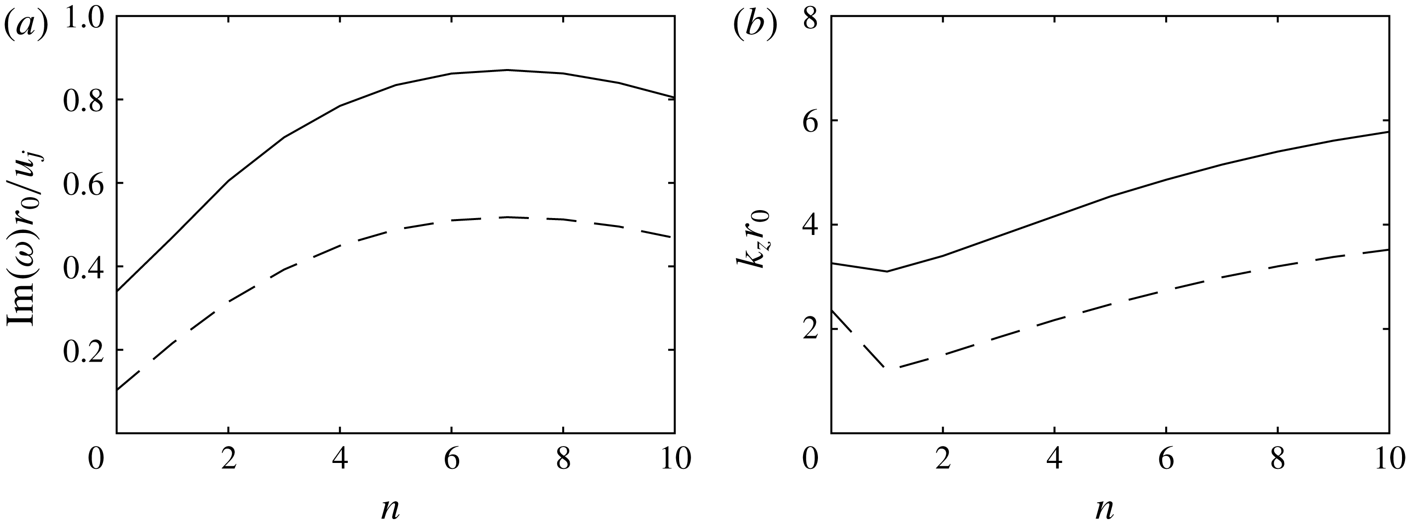
Representation of the (a) maximum amplification rate and (b) the most amplified axial wavenumber as a function of the azimuthal mode number for ——
 $M_{j}=2$
and - - - -
 $M_{j}=3$
.

An inviscid temporal stability analysis is carried out from the initial velocity and density profiles. For a given axial wavenumber
 $k_{z}$
and azimuthal mode
 $n$
, the compressible Rayleigh equation is solved in cylindrical coordinates using a shooting method. This method combines the Euler method for the integration step and the secant method for the search of the complex angular frequency
 $\unicode[STIX]{x1D714}$
. The integration in the radial direction is performed on an homogeneous grid with a spacing of
 $0.0001r_{0}$
, extending from the LES point closest to the jet axis out to
 $r=5r_{0}$
.
The amplification rates of the Kelvin–Helmholtz instability waves obtained for the first five azimuthal modes are represented in figure 1 as a function of the axial wavenumber for the two jets. For each azimuthal mode, they are positive over a broad range of axial wavenumbers, and reach maximum values over
 $3\leqslant k_{z}r_{0}\leqslant 5$
at Mach 2 and over
 $2\leqslant k_{z}r_{0}\leqslant 3$
at Mach 3. The peak amplification rates and their corresponding axial wavenumbers are plotted in figure 2 as a function of the mode number. For the two jets, the most amplified mode is mode
 $n=7$
. For this mode, the maximum amplification rate is obtained for
 $k_{z}r_{0}=5.2$
at Mach 2, and for
 $k_{z}r_{0}=3$
at Mach 3, yielding wavelengths of
 $1.2r_{0}$
and
 $2.1r_{0}$
, respectively. Furthermore, for all azimuthal mode numbers, the maximum amplification rate is lower, and is reached for lower values of the axial wavenumber at Mach 2 than at Mach 3. This well-known effect of compressibility on the Kelvin–Helmholtz instability waves is expected to cause the Mach 3 jet to grow at a slower rate, and to exhibit stronger low-wavenumber components in the early stages of its development than the Mach 2 jet.
3 Simulation results
3.1 Flow development
3.1.1 Vorticity field
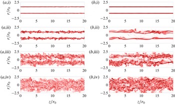
Instantaneous fields of the vorticity norm are represented in figure 3 for the two jets at times
 $t=5r_{0}/u_{j}$
,
 $t_{c}-10r_{0}/u_{j}$
,
 $t_{c}$
and
 $t_{c}+10r_{0}/u_{j}$
, where
 $t_{c}$
is the time of the potential core closure. This time, defined as the time when the mean centreline velocity reaches the value of
 $0.95u_{j}$
, is equal to
 $25.3r_{0}/u_{j}$
for the jet at
 $M_{j}=2$
and to
 $61.1r_{0}/u_{j}$
for the jet at
 $M_{j}=3$
. At
 $t=5r_{0}/u_{j}$
, the vorticity is concentrated in thin axisymmetric mixing layers separating the inner potential core of the jet and the ambient medium. Very slight perturbations are distinguishable in the mixing layers and correspond to the instability waves growing from the initial excitation. At
 $t=t_{c}-10r_{0}/u_{j}$
, the mixing layers are thicker than previously, due to the development of turbulent structures. The mixing layers of the Mach 3 jet exhibit larger scales than those of the Mach 2 jet, which is consistent with the linear stability analysis predicting that the most amplified axial wavenumber is lower at a higher Mach number. At
 $t=t_{c}$
, the mixing layers from the opposite sides of the jet begin to interact on the centreline. Finally, the jets are fully mixed at
 $t_{c}+10r_{0}/u_{j}$
.
Vorticity norm for (a)
 $M_{j}=2$
and (b)
 $M_{j}=3$
at times (i)
 $t=5r_{0}/u_{j}$
, (ii)
 $t_{c}-10r_{0}/u_{j}$
, (iii)
 $t_{c}$
and (iv)
 $t_{c}+10r_{0}/u_{j}$
. The colour scale ranges from 0 to
 $5u_{j}/r_{0}$
, from white to red.

3.1.2 Mean and fluctuating axial velocity fields
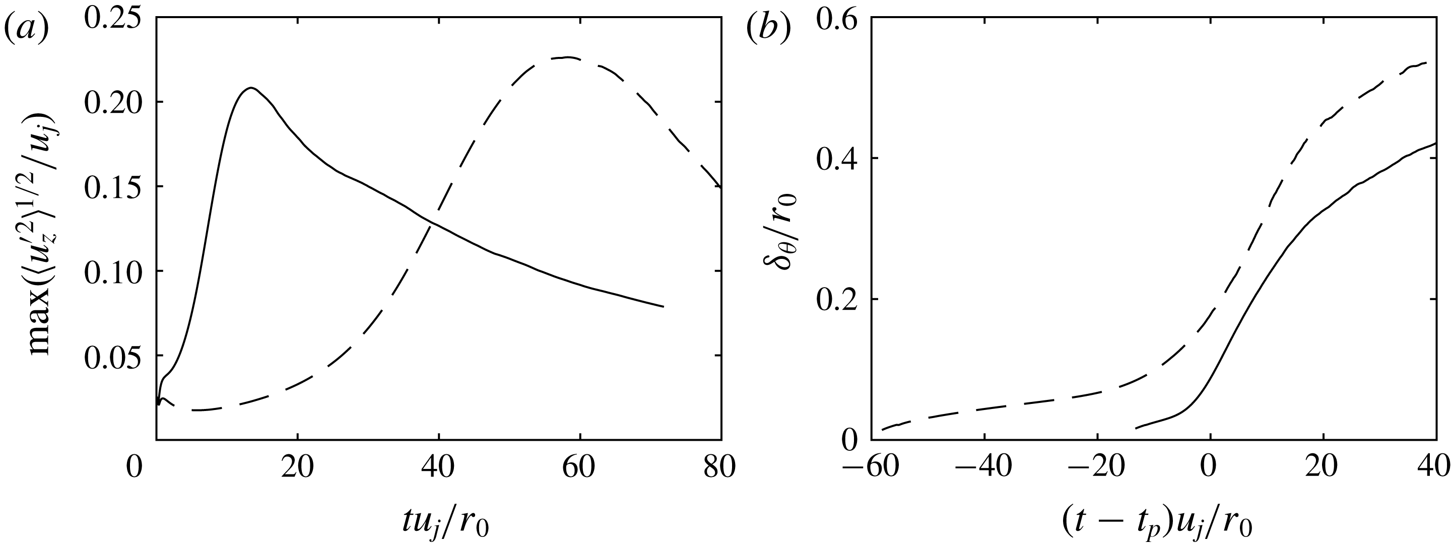
The time variations of the maximum root-mean-square (r.m.s.) values of axial velocity fluctuations are presented in figure 4(a). For the two jets, the velocity fluctuations start at
 $t=0$
at a value close to 2 % of the jet velocity and then rise and reach a peak at a time
 $t_{p}=13.4r_{0}/u_{j}$
for
 $M_{j}=2$
and
 $t_{p}=58.2r_{0}/u_{j}$
for
 $M_{j}=3$
. The peak value is approximately equal to 20 % of the jet initial velocity and can be attributed (Bogey & Bailly Reference Bogey and Bailly2010) to the pairing of vortices when the jet shear layers transition from a laminar to a turbulent state. This time
 $t_{p}$
will be used as a reference throughout the paper to perform comparison between the two jets. It is longer for the Mach 3 jet than for the Mach 2 jet, which can be explained by the lower growth rate of instability waves in the former case.
The shear-layer momentum thicknesses are represented in figure 4(b) as a function of
 $t-t_{p}$
. Initially, it grows slowly as the shear layers are in a laminar state. At
 $t\simeq t_{p}$
, as the jets transition from a laminar to a turbulent state, the momentum thickness rapidly increases and grows at a fast pace until the closing of the potential core, when the mixing layers join and merge on the jet axis. Then, the momentum thickness continues to grow, but at a slower rate.
Time variations of (a) maximum r.m.s. value of axial velocity fluctuations and (b) shear-layer momentum thickness for ——
 $M_{j}=2$
and - - - -
 $M_{j}=3$
.

3.1.3 Spectra of velocity fluctuations
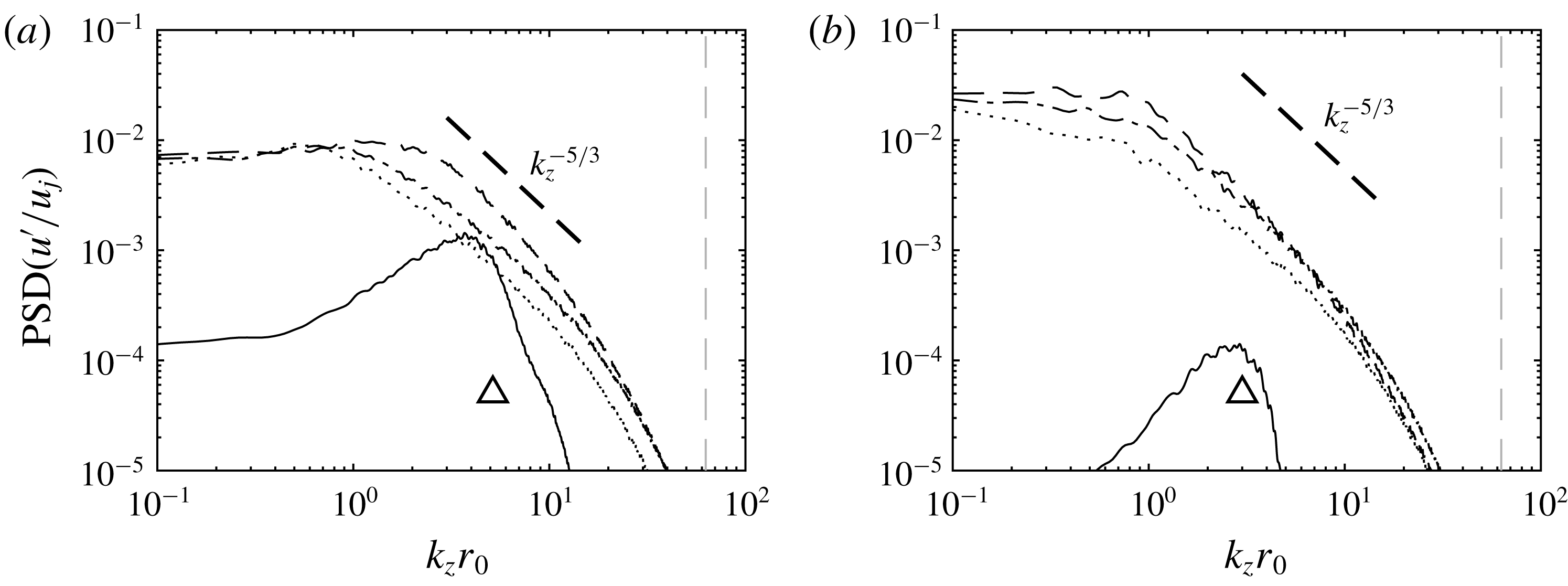
Representation, for (a)
 $M_{j}=2$
and (b)
 $M_{j}=3$
, of the power spectral densities of axial velocity fluctuations at
 $r=r_{0}$
normalised by
 $u_{j}$
as a function of the axial wavenumber at times ——
 $5r_{0}/u_{j}$
, - - - -
 $t_{p}$
, — ⋅ —
 $t_{p}+10r_{0}/u_{j}$
and
 $\cdots \cdots$
 $t_{p}+20r_{0}/u_{j}$
. The triangle indicates the most amplified wavenumber at
 $t=0$
and the dashed grey line indicates the grid cutoff wavenumber.

Representation, for (a)
 $M_{j}=2$
and (b)
 $M_{j}=3$
, of the power spectral densities of axial velocity fluctuations at
 $r=r_{0}$
normalised by
 $u_{j}$
as a function of the azimuthal mode number at times ——
 $5r_{0}/u_{j}$
, - - - -
 $t_{p}$
, — ⋅ —
 $t_{p}+10r_{0}/u_{j}$
and
 $\cdots \cdots$
 $t_{p}+20r_{0}/u_{j}$
. The triangle indicates the most amplified mode number at
 $t=0$
.

The power spectral densities of the axial velocity fluctuations at
 $r=r_{0}$
at
 $t=5r_{0}/u_{j}$
,
 $t_{p}-10r_{0}/u_{j}$
,
 $t_{p}$
and
 $t_{p}+10r_{0}/u_{j}$
are represented in figure 5 as a function of the axial wavenumber. The grid cutoff wavenumber
 $k_{z}r_{0}=62.8$
is also displayed. At
 $t=5r_{0}/u_{j}$
, as the jet mixing layers are still in a laminar state, the spectra obtained for the two jets display a distinctive hump close to the most unstable wavenumber predicted from linear stability analysis, i.e. for
 $k_{z}r_{0}=5.2$
at
 $M_{j}=2$
and for
 $k_{z}r_{0}=3$
at
 $M_{j}=3$
. In appendix A, this peak wavenumber is shown not to depend on the strength of the initial forcing. At
 $t=t_{p}$
, when the jets transition to a turbulent state, the spectra are broadband thanks to the presence of turbulent fluctuations in the jet shear layers. At subsequent times, for
 $t=t_{p}+10r_{0}/u_{j}$
and
 $t_{p}+20r_{0}/u_{j}$
, the spectra display a similar shape to that at
 $t=t_{p}$
. Moreover, at
 $t=t_{p}+20r_{0}/u_{j}$
, the spectral slopes are close to the
 $k_{z}^{-5/3}$
slope characteristic of turbulence at equilibrium over a little less than one wavenumber decade. Further later, at
 $t=t_{p}+55r_{0}/u_{j}$
for instance, the spectra, not shown for brevity, display a wider inertial range because of the fully developed state of the turbulence at these times.
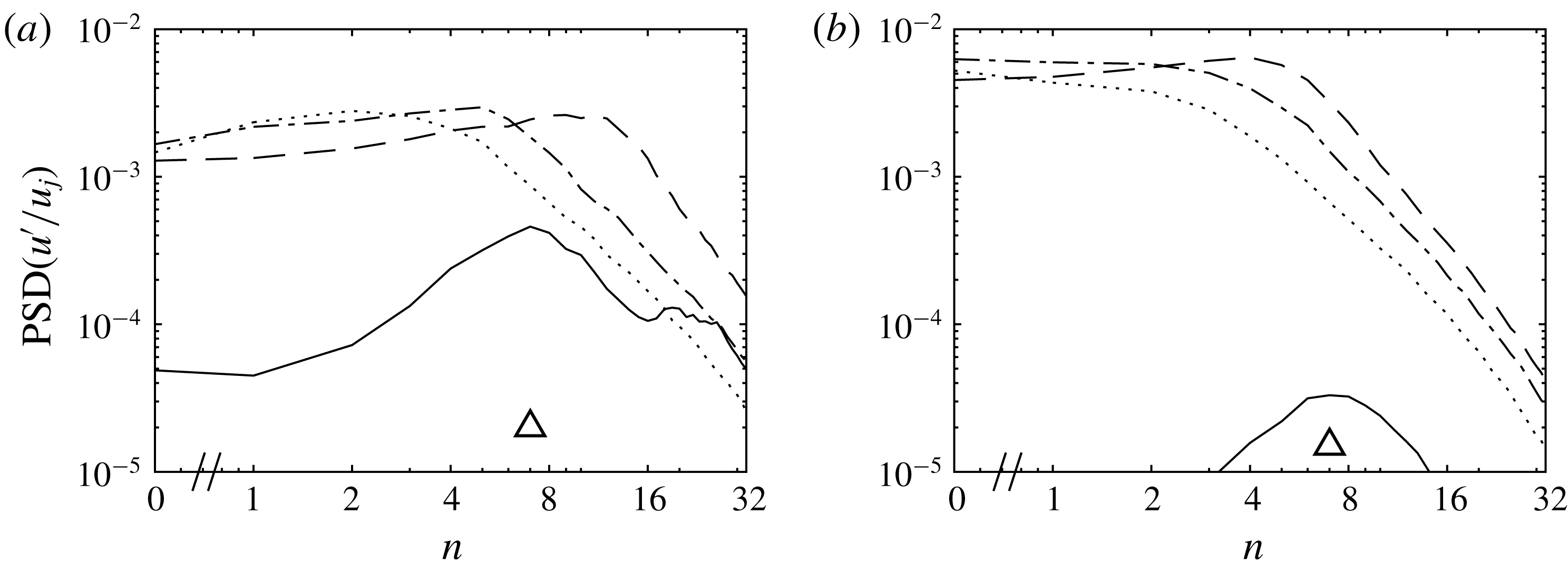
The azimuthal power spectral densities of axial velocity fluctuations computed at
 $r=r_{0}$
are shown in figure 6 as a function of the azimuthal mode number
 $n$
at the same times as the spectra in figure 5. At
 $t=5r_{0}/u_{j}$
, the most energetic mode is the seventh azimuthal mode, which is also the most amplified one based on the linear stability analysis. At later times, the spectra are broader, following the jet transition from a laminar to a turbulent state, which causes the formation of turbulent fluctuations over a wide range of mode numbers. The peak mode number also decreases over time, as visible in the spectra at
 $t=t_{p}+10r_{0}/u_{j}$
and
 $t_{p}+20r_{0}/u_{j}$
.
3.2 Near pressure field
3.2.1 Statistical properties of the near pressure field
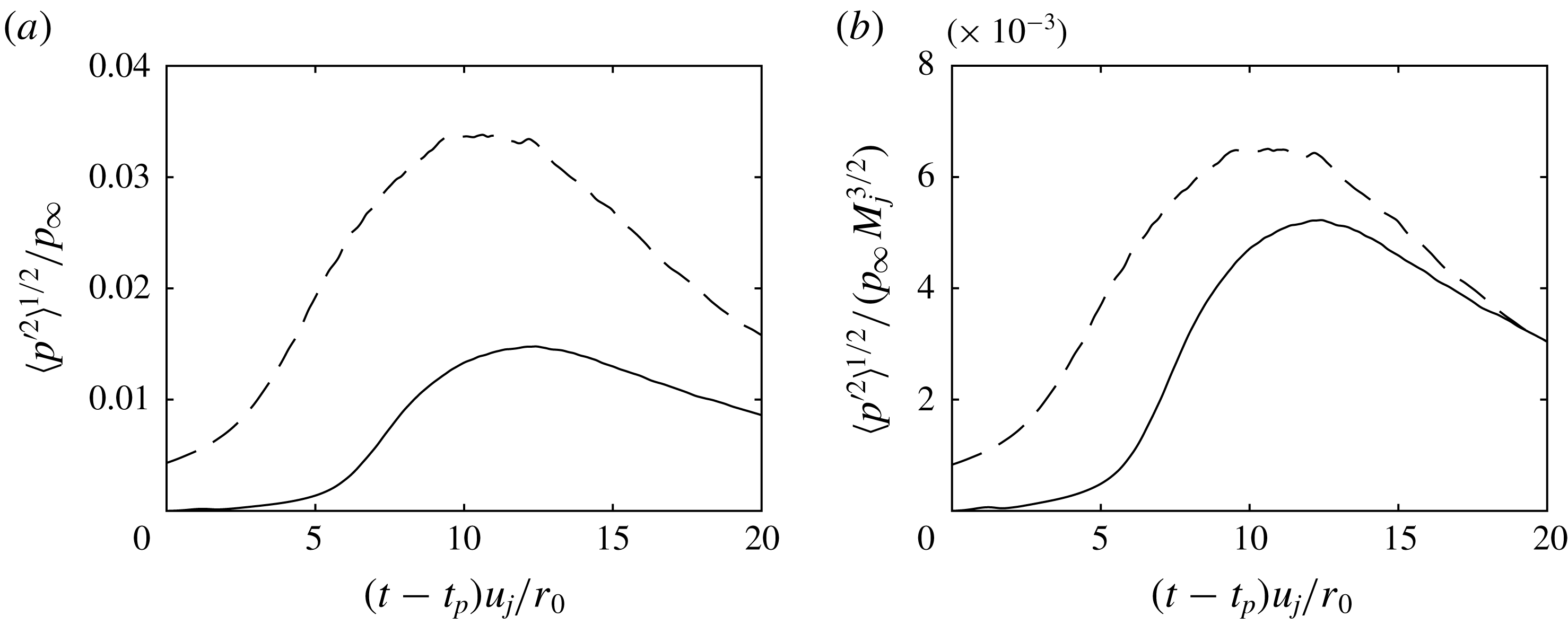
The time variations of the r.m.s. value of pressure fluctuations at
 $r=8r_{0}$
are plotted in figure 7(a). For the two jets, a peak is reached at
 $t\simeq t_{p}+12r_{0}/a_{\infty }$
, due to the generation of intense acoustic waves during the development of the jets. The peak pressure is stronger for the Mach 3 jet than for the Mach 2 jet, as expected, which is due to the higher speed of the former. In addition, when normalised by
 $M_{j}^{3/2}$
, the peak pressure levels do not significantly differ in figure 7(b), which is consistent with a common assumption that the sound intensity produced by supersonic jets varies with the third power of the jet speed (Ffowcs Williams Reference Ffowcs Williams1963). After the peak, the pressure fluctuations gradually weaken over time, following the decrease of the velocity fluctuation intensity.
Time variations of the r.m.s. value of pressure fluctuations at
 $r=8r_{0}$
normalised by (a)
 $p_{\infty }$
and (b)
 $p_{\infty }M_{j}^{3/2}$
for ——
 $M_{j}=2$
and - - - -
 $M_{j}=3$
.

Snapshots of pressure fluctuations and vorticity norm at
 $t=t_{p}+12r_{0}/a_{\infty }$
for (a)
 $M_{j}=2$
and (b)
 $M_{j}=3$
. The colour scales range from
 $-0.02p_{\infty }M_{j}^{3/2}$
to
 $0.02p_{\infty }M_{j}^{3/2}$
for the pressure and up to
 $3u_{j}/r_{0}$
for the vorticity, from blue to red.

Values at
 $r=8r_{0}$
and
 $t=t_{p}+12r_{0}/a_{\infty }$
of the normalised skewness
 $S$
and kurtosis
 $K$
of the pressure
 $p$
and dilatation
 $\unicode[STIX]{x1D6E9}$
.

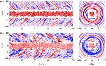
Snapshots of the pressure fluctuations and vorticity fields in the
 $(r,z)$
and
 $(r,\unicode[STIX]{x1D703})$
planes are provided in figure 8 at the time
 $t_{p}+12r_{0}/a_{\infty }$
of peak levels for
 $r=8r_{0}$
, as well as in the corresponding movies movie_figure8a and movie_figure8b available online at https://doi.org/10.1017/jfm.2019.729 for
 $M_{j}=2$
and
 $M_{j}=3$
, respectively. In the
 $(r,z)$
plane, straight, elongated wavefronts propagating in the downstream direction are observed in the vicinity of the flow. They are very similar to the Mach waves observed in simulations (de Cacqueray et al.
Reference de Cacqueray, Bogey and Bailly2011; Nichols et al.
Reference Nichols, Lele and Spyropoulos2013b
), as well as in optical visualisations (Lowson & Ollerhead Reference Lowson and Ollerhead1968; Kearney-Fischer, Kim & Samimy Reference Kearney-Fischer, Kim and Samimy2011; Murray & Lyons Reference Murray and Lyons2016) for spatially developing supersonic jets. In addition, the snapshots in the
 $(r,\unicode[STIX]{x1D703})$
plane reveal organised wavefronts spanning the entire circumference of the jets, highlighting the strong azimuthal correlation of the sound field. Some of the waves in the snapshots of figure 8 have an asperous, jagged aspect, especially in the case of the Mach 3 jet, which indicates the presence of shock-like, steepened waves. As in the study of Nichols et al. (Reference Nichols, Lele, Ham, Martens and Spyropoulos2013a
), these fast compression waves are visible in the immediate vicinity of the jet flow and appear to be associated with the coherent, elongated Mach waves that dominate the sound field. They also appear to be significantly correlated in the azimuthal direction, which will be investigated into further details later on in the paper.
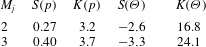
In the past, several statistical indicators have been proposed in order to quantify the presence of such steepened waves (Ffowcs Williams Reference Ffowcs Williams1963; McInerny Reference McInerny1997; Krothapalli, Arakeri & Greska Reference Krothapalli, Arakeri and Greska2003; Falco Reference Falco2007; Baars & Tinney Reference Baars and Tinney2014). Notably, the skewness and kurtosis factors provide useful information on the asymmetry and intermittency of the sound field (Ffowcs Williams et al.
Reference Ffowcs Williams, Simson and Virchis1975; Mora et al.
Reference Mora, Heeb, Kastner, Gutmark and Kailasanath2014; Fiévet et al.
Reference Fiévet, Tinney, Baars and Hamilton2016). Their values, computed at
 $r=8r_{0}$
and at
 $t=t_{p}+12r_{0}/a_{\infty }$
for the pressure and dilatation fields, are reported in table 1. For both jets, the skewness and kurtosis factors of the pressure fluctuations are significantly higher than the values 0 and 3 expected for a Gaussian distribution, as observed in jets emitting crackle noise. In addition, the skewness factor of the dilatation is negative, while its kurtosis factor takes large, positive values, revealing the intermittent presence of strong, shock-like compressions in the signals. As expected, the present indicators are stronger, in absolute value, at Mach 3 than at Mach 2, which shows that the waves generated by the jets are steeper, more positively skewed and more intermittent at the highest Mach number.
Pressure fluctuation spectra at
 $t=t_{p}+12r_{0}/a_{\infty }$
normalised by
 $p_{\infty }M_{j}^{3}$
as a function of (a) axial wavenumber and (b) azimuthal mode number for ——
 $M_{j}=2$
and - - - -
 $M_{j}=3$
.

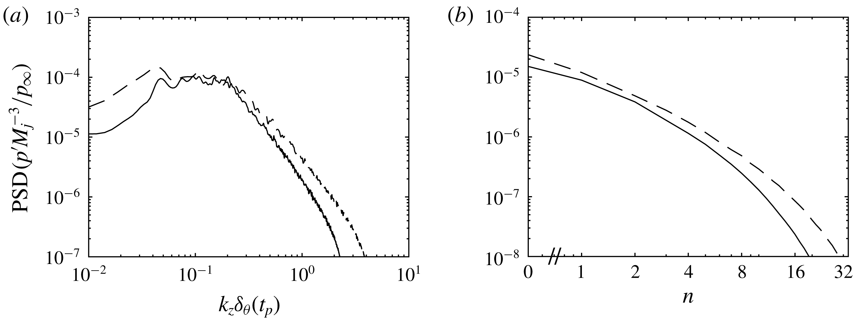
In order to explore the structure of the sound field from a more quantitative perspective, axial and azimuthal power spectral densities of pressure fluctuations obtained at
 $r=8r_{0}$
at
 $t=t_{p}+12r_{0}/a_{\infty }$
are shown in figure 9. They are normalised by
 $p_{\infty }M_{j}^{3}$
, following the assumption that sound intensity varies with the third power of the jet speed. In figure 9(a), the spectra are plotted as a function of
 $k_{z}\unicode[STIX]{x1D6FF}_{\unicode[STIX]{x1D703}}(t_{p})$
, where
 $\unicode[STIX]{x1D6FF}_{\unicode[STIX]{x1D703}}(t_{p})$
is the shear-layer momentum thickness at time
 $t_{p}$
, and is equal to
 $0.09r_{0}$
for
 $M_{j}=2$
, and to
 $=0.18r_{0}$
for
 $M_{j}=3$
. This choice is motivated by the expectation that the dominant wavelength in the pressure field should scale according to the shear-layer thickness at time of peak noise emission, arbitrarily estimated as
 $t=t_{p}$
. The reasonably good collapse of the spectra confirms this assumption. In particular, they both peak for a wavenumber
 $k_{z}\unicode[STIX]{x1D6FF}_{\unicode[STIX]{x1D703}}(t_{p})\simeq 0.2$
, yielding acoustic wavelengths of approximately
 $2.8r_{0}$
for
 $M_{j}=2$
and
 $5.7r_{0}$
for
 $M_{j}=3$
. The collapse is however less obvious at low and high wavenumbers, where the pressure levels are higher for
 $M_{j}=3$
than for
 $M_{j}=2$
. In the high-wavenumber range, this excess is due to the presence of more shock-like structures in the jet near field, as indicated by the skewness and kurtosis factors in table 1. Indeed, the sharp compressions associated with these structures are expected to cause an increase of the energy contained in high-wavenumber components. In the low-wavenumber range, the discrepancy is likely to be due to the presence of low-frequency, hydrodynamic components whose spectra are not expected to scale according to
 $M_{j}^{3}$
(Arndt, Long & Glauser Reference Arndt, Long and Glauser1997).
The pressure power spectral densities are also plotted as a function of the azimuthal mode number in figure 9(b). In all cases, the dominant azimuthal mode number is the axisymmetric one, and the energy decay is rapid at higher mode numbers. In particular, 87 % of the total sound intensity radiated by the Mach 2 jet is contained within the azimuthal modes of order 0 to 4 whereas 82 % of the total intensity is contained within these modes for the Mach 3 jet. The results are in agreement with experimental (Troutt & McLaughlin Reference Troutt and McLaughlin1982) and numerical (de Cacqueray et al. Reference de Cacqueray, Bogey and Bailly2011; Sinha et al. Reference Sinha, Rodriguez, Brès and Colonius2014) studies of spatially developing supersonic jets, where low-order azimuthal modes are prevalent in the noise radiated in the downstream direction.
3.2.2 Azimuthal structure of the steepened waves
Profiles of pressure fluctuations at
 $r=8r_{0}$
at
 $t=t_{p}+12r_{0}/a_{\infty }$
for
 $M_{j}=2$
; partial sum of the azimuthal modes from mode 0 to mode
 $N$
, with ——
 $N=0$
, - - - -
 $N=1$
, — ⋅ —
 $N=2$
,
 $\cdots \cdots$
 $N=3$
and —— (grey)
 $N=4$
and —— full signal.

Pressure fluctuation spectra at
 $r=8r_{0}$
at
 $t=t_{p}+12r_{0}/a_{\infty }$
for (a)
 $M_{j}=2$
and (b)
 $M_{j}=3$
; partial sum of the azimuthal modes from mode 0 to mode
 $N$
, with - - - -
 $N=0$
, — ⋅ —
 $N=1$
and
 $\cdots \cdots$
 $N=4$
and —— full signal.

In order to illustrate the main features of the steepened waves radiated by the jets, the pressure fluctuations obtained at
 $r=8r_{0}$
at
 $t=t_{p}+12r_{0}/a_{\infty }$
are provided in figure 10. Two steepened, shock-like waves are clearly visible at
 $z=223.6r_{0}$
and
 $z=226r_{0}$
. Their shapes are typical of the structures observed near jets radiating crackle noise. In particular, a rapid compression phase yields to a strong positive pressure peak and it is followed by a gradual expansion having a much wider extent than the initial compression, spanning approximately over
 $2r_{0}$
. The pressure profiles reconstructed from all of the
 $N\text{th}$
first azimuthal modes, with
 $N$
ranging from 0 to 4 are also plotted in figure 10. Rapid compressions are not found in the waveforms obtained for
 $N=0$
, when only the axisymmetric mode is considered. Rather, the compressions associated with the shocks are progressively unveilled as more modes are included in the reconstruction of the pressure field. In particular, for
 $N=4$
, all of the most important features of the full field are present, including the sharp compression waves.
The power spectral densities of the signals reconstructed from the
 $N\text{th}$
first azimuthal modes are plotted for
 $N=0$
,
 $1$
and
 $4$
in figure 11, as a function of the axial wavenumber. For the two jets, the spectra for
 $N=0$
closely match those for the full fields at very low wavenumbers but significantly differ for
 $k_{z}r_{0}\geqslant 0.1$
. For instance, for
 $M_{j}=2$
, the axisymmetric mode contains more than 95 % of the total sound intensity for
 $k_{z}\unicode[STIX]{x1D6FF}_{\unicode[STIX]{x1D703}}=0.1$
, but only 10 % for
 $k_{z}\unicode[STIX]{x1D6FF}_{\unicode[STIX]{x1D703}}=0.5$
. The agreement between the reconstructed and full pressure fields is satisfactory over a wider range of wavenumbers as more modes are included in the reconstruction. For
 $N=4$
, the spectra obtained for the reconstructed field closely match those for the full field up to
 $k_{z}\unicode[STIX]{x1D6FF}_{\unicode[STIX]{x1D703}}(t_{p})\simeq 0.6$
although significant differences persist in the high-wavenumber range, for
 $k_{z}\unicode[STIX]{x1D6FF}_{\unicode[STIX]{x1D703}}(t_{p})\geqslant 1$
for instance. However, based on the analysis of the waveforms in figure 10, the missing, high-wavenumber components associated with modes higher than 4 are not expected to significantly change the structure of steepened waves, whose most peculiar features are associated with low-order modes. For that reason, the following study of their generation process is limited to the azimuthal reconstruction of the flow and sound fields with
 $N=4$
. This should facilitate the analysis by filtering out the contribution of these high-order azimuthal modes.
3.3 Mechanisms at the origin of the steepened waves
3.3.1 Conditional averages of the wave generation process
Axial profiles of the conditionally averaged pressure at
 $t=t_{trig}$
and
 $r=r_{trig}$
for (a)
 $M_{j}=2$
and (b)
 $M_{j}=3$
; azimuthal modes ——
 $n=0$
, - - - -
 $n=1$
, — ⋅ —
 $n=2$
,
 $\cdots \cdots$
 $n=3$
and —— (grey)
 $n=4$
.

In order to investigate the mechanisms leading to the generation of steepened waves, a conditional averaging procedure is applied to the flow and sound fields of the jets. This technique consists in synchronising several flow events over a detection criterion, before performing an ensemble average such that only recurrent, generic features remain (Antonia Reference Antonia1981). When the trigger condition is related to the acoustic pressure field, conditional averages constitute a powerful tool for the study of sound generation mechanisms since they allow flow events associated with noise production to be described (Mercier, Castelain & Bailly Reference Mercier, Castelain and Bailly2018; Bogey Reference Bogey2019; Schmidt & Schmid Reference Schmidt and Schmid2019). In the present study, the conditional averages are triggered by the detection of extreme maxima of pressure fluctuations at a distance
 $r_{trig}=4.5r_{0}$
from the jet axis, in the very near acoustic field. This location has been empirically chosen to be far enough from the flow that acoustic disturbances are dominant in the pressure field but close enough that nonlinear propagation effects have only a weak impact on the acoustic waves. The profiles of pressure fluctuations obtained at time
 $t_{trig}=t_{p}+6r_{0}/a_{\infty }$
, close to the time of peak pressure levels at
 $r=r_{trig}$
, are binned in intervals of length
 $30\unicode[STIX]{x1D6FF}_{\unicode[STIX]{x1D703}}(t_{p})$
in the axial direction, corresponding to an axial wavenumber
 $k_{z}\unicode[STIX]{x1D6FF}_{\unicode[STIX]{x1D703}}(t_{p})\simeq 0.2$
, close to the peak of the spectra in figure 9. For each interval, the pressure maximum is determined, and the flow and sound fields are synchronised according to the axial and azimuthal coordinates of peak pressure, labelled
 $z_{trig}$
and
 $\unicode[STIX]{x1D703}_{trig}$
, and ensemble averaged.
The conditional averaging procedure is first applied to individual azimuthal modes of the pressure field, as in the study of Schmidt & Schmid (Reference Schmidt and Schmid2019). For the two jets, the axial variations of the waveforms obtained at
 $t=t_{trig}$
and
 $r=r_{trig}$
are shown in figure 12 for the first five azimuthal modes. The signals are normalised by
 $M_{j}^{3/2}$
and plotted as a function of
 $(z-z_{trig})/\unicode[STIX]{x1D6FF}_{\unicode[STIX]{x1D703}}(t_{p})$
, using the same length scale reference as for the spectra in figure 9. For the two jets, and for all mode numbers, the conditionally averaged pressure fluctuations are maximum for
 $z=z_{trig}$
, as expected given the synchronisation condition. Moreover, they remain positive over a distance which shortens with the mode number, and equal to approximately ten times the shear-layer momentum thickness. It is noteworthy that none of the waveforms exhibits sharp compressions such as those in the signals reconstructed from the first five modes in figure 10. Instead, the conditional pressure fluctuations obtained for all mode numbers are symmetric with respect to the trigger position
 $z_{trig}$
. This shows that steepened waves are not associated with one particular azimuthal mode of the pressure field, and suggests that several modes need to be superposed in order to recover their specific features.
Axial profiles of the conditionally averaged pressure in the plane
 $\unicode[STIX]{x1D703}=\unicode[STIX]{x1D703}_{trig}$
at
 $t=t_{trig}$
and
 $r=r_{trig}$
for (a)
 $M_{j}=2$
and (b)
 $M_{j}=3$
; partial sum up to order
 $N$
with ——
 $N=0$
, - - - -
 $N=1$
, — ⋅ —
 $N=2$
,
 $\cdots \cdots$
 $N=3$
and —— (grey)
 $N=4$
.

On the basis of the above finding, the conditional averaging procedure is now applied to the pressure field reconstructed from all of the azimuthal modes of order ranging from
 $n=0$
to 4. They are computed from 142 and 110 shock events for the jets at Mach 2 and 3, respectively, and this number is shown in appendix B to be sufficient to obtain converged statistics. The axial variations of the conditional waveforms at
 $r_{trig}$
and
 $t_{trig}$
are provided in figure 13 for the two Mach numbers, using the same normalisation as in figure 12. The partial sum of the azimuthal modes up to the order
 $N$
is also represented for
 $0\leqslant N\leqslant 4$
, in order to highlight the contribution of the different modes. The steepened, asymmetric shape of the waveforms is clearly visible in the present conditional averages, and it is more pronounced as more azimuthal modes are included. Notably, the sharp compression and smooth expansion are observed for
 $N=4$
, confirming that only five modes are sufficient to recover the main features of the steepened shock-like waves. The peak of the conditional pressure does not scale according to the third power of the jet velocity, as the normalised pressure maximum is equal to 0.02 for
 $M_{j}=2$
and to 0.03 for
 $M_{j}=3$
. This suggests that the conditional averages are computed from more extreme events at
 $M_{j}=3$
than at
 $M_{j}=2$
, which is consistent with the higher skewness and kurtosis obtained for the former Mach number.
Conditionally averaged pressure at
 $r=r_{trig}$
and
 $t=t_{trig}$
for
 $M_{j}=2$
represented in the plane ——
 $\unicode[STIX]{x1D703}=\unicode[STIX]{x1D703}_{trig}$
, - - - -
 $\unicode[STIX]{x1D703}_{trig}+\unicode[STIX]{x03C0}/6$
, — ⋅ —
 $\unicode[STIX]{x1D703}_{trig}+\unicode[STIX]{x03C0}/3$
and
 $\cdots \cdots$
 $\unicode[STIX]{x1D703}_{trig}+\unicode[STIX]{x03C0}/2$
.

The azimuthal structure of the waves is illustrated in figure 14, where the conditional waveforms reconstructed from
 $N=4$
for the jet at
 $M_{j}=2$
are represented in the planes
 $\unicode[STIX]{x1D703}=\unicode[STIX]{x1D703}_{trig}$
,
 $\unicode[STIX]{x1D703}_{trig}+\unicode[STIX]{x03C0}/6$
,
 $\unicode[STIX]{x1D703}_{trig}+\unicode[STIX]{x03C0}/3$
and
 $\unicode[STIX]{x1D703}_{trig}+\unicode[STIX]{x03C0}/2$
. As expected, the pressure is strongest in the detection plane at
 $\unicode[STIX]{x1D703}_{trig}$
, but rapidly decreases with increasing azimuthal angle, so that the levels obtained for
 $\unicode[STIX]{x1D703}=\unicode[STIX]{x1D703}_{trig}+\unicode[STIX]{x03C0}/2$
are more than ten times lower than the maximum pressure. The waveforms are also smoother at a higher azimuthal angle, which indicates that the sharp compressions associated with the waves are localised over a narrow azimuthal extent centred around the detection angle
 $\unicode[STIX]{x1D703}_{trig}$
.
Conditional averages in the detection plane
 $\unicode[STIX]{x1D703}=\unicode[STIX]{x1D703}_{trig}$
are also computed at times
 $t<t_{trig}$
to provide a chronological description of the events leading to the formation of the steepened waves. Two-dimensional plane views of the conditional pressure and radial velocity fields are shown in figure 15 at times
 $t=t_{p}+1.5r_{0}/a_{\infty }$
,
 $t_{p}+3r_{0}/a_{\infty }$
,
 $t_{p}+4.5r_{0}/a_{\infty }$
and
 $t_{p}+6r_{0}/a_{\infty }$
; see also the corresponding movies movie_fig15a and movie_fig15b. The sonic line, defined as
 $u_{z}=a_{\infty }$
, is also represented to highlight the upper limit of the jet supersonic core. The conditional flow and sound fields obtained for the two Mach numbers are very similar. At
 $t_{p}+1.5r_{0}/a_{\infty }$
, a straight, inclined pressure wave emerges from the jet, upstream of
 $z=z_{trig}$
. It consists of a positive peak surrounded by two bands of negative levels, and its shape reminds us that of wavepacket disturbances extracted from simulations of spatial supersonic jets by Sinha et al. (Reference Sinha, Rodriguez, Brès and Colonius2014), for instance. Inside the jet flow, the inner tip of this pressure disturbance is directly connected to a large-scale perturbation of the radial velocity, located in the inner, supersonic core of the jet. A slight indentation of the sonic line is associated with this disturbance. At
 $t_{p}+3r_{0}/a_{\infty }$
, the inner tip of the wave remains connected to the velocity disturbance, which is still located in the supersonic side of the jet, but downstream from its initial position. Finally, for
 $t_{p}+4.5r_{0}/a_{\infty }$
and
 $t_{p}+6r_{0}/a_{\infty }$
, the wave separates from the flow and propagates in the downstream direction.
Conditionally averaged pressure and radial velocity fluctuations for (a)
 $M_{j}=2$
and (b)
 $M_{j}=3$
at times (i)
 $t_{p}+1.5r_{0}/a_{\infty }$
, (ii)
 $t_{p}+3r_{0}/a_{\infty }$
, (iii)
 $t_{p}+4.5r_{0}/a_{\infty }$
and (iv)
 $t_{p}+6r_{0}/a_{\infty }$
. The dashed line indicates the sonic line and the colour scales range from
 $-0.03p_{\infty }M_{j}^{3/2}$
to
 $0.03p_{\infty }M_{j}^{3/2}$
for the pressure and up to
 $0.1u_{j}$
for the radial velocity, from blue to red.

The inclination angle
 $\unicode[STIX]{x1D6FC}_{cond}$
of the waves can be estimated from the orientation of the pressure gradient, computed at the location of minimum dilatation. At time
 $t_{trig}$
, this yields
 $\unicode[STIX]{x1D6FC}_{cond}=46^{\circ }$
for
 $M_{j}=2$
and
 $53^{\circ }$
for
 $M_{j}=3$
. Thus, the acoustic waves radiated by the jet at
 $M_{j}=3$
are more inclined than at
 $M_{j}=2$
, which can be related to the higher convection speed in the latter case. This speed can be estimated from the relation
 $$\begin{eqnarray}u_{c}=\frac{a_{\infty }}{\cos \unicode[STIX]{x1D6FC}_{cond}},\end{eqnarray}$$
leading to
 $u_{c}=1.5a_{\infty }$
for
 $M_{j}=2$
and
 $1.7a_{\infty }$
, for
 $M_{j}=3$
. These values can be compared with those obtained from the axial position of the minimum of radial velocity in the lower, high-speed part of the jet. This position, shown in figure 16 varies approximately linearly, indicating a nearly constant convection speed, close to
 $u_{c}=0.7u_{j}=1.4a_{\infty }$
for
 $M_{j}=2$
and to
 $0.55u_{j}=1.65a_{\infty }$
for
 $M_{j}=3$
, which are in good agreement with those estimated from the wavefront inclinations. This strongly suggests that the waves in the conditional averages are Mach waves produced by the flow large-scale coherent structures. This is further supported by the variations of the location of peak conditional pressure, also represented in figure 16. This location is indeed very similar to that of the minimum of radial velocity from
 $t_{p}$
to
 $t_{p}+3r_{0}/a_{\infty }$
, i.e. when the pressure wave is attached to the flow disturbance. This is not true for
 $t\geqslant t_{p}+4r_{0}/a_{\infty }$
, when the wave separates from the flow disturbance and propagates away from the jet. During that time, the position of the peak pressure still increases linearly, but at a speed close to the value of
 $a_{\infty }\cos \unicode[STIX]{x1D6FC}_{cond}$
obtained assuming a propagation in the direction predicted from (3.1).
The present conditional averages thus show a direct link between the formation of steepened waves and the supersonic convection of large-scale flow disturbances located inside the jets. These flow disturbances have supersonic convection speeds, persist over significant length and time scales, and bear some resemblance to large-scale coherent structures extracted in jets at lower speed (Yule Reference Yule1978; Bogey Reference Bogey2019). This provides evidence that steepened waves generated by supersonic jets are a particular, nonlinear case of Mach wave radiations by coherent structures, as proposed in previous studies (Nichols et al. Reference Nichols, Lele, Ham, Martens and Spyropoulos2013a ; Murray & Lyons Reference Murray and Lyons2016; Buchta & Freund Reference Buchta and Freund2017). Given their nonlinear nature, steepened waves only appear when several azimuthal modes are simultaneously considered and thus cannot be related to one particular, azimuthal mode.
Time evolution of the axial positions of —— minimum radial velocity and - - - - maximum pressure in the plane at
 $\unicode[STIX]{x1D703}=\unicode[STIX]{x1D703}_{trig}$
for (a)
 $M_{j}=2$
and (b)
 $M_{j}=3$
.

3.3.2 Flow events at the origin of the steepened waves
The connection between the steepened waves and the flow disturbances is further explored in order to determine what particular aspect of the flow structures causes Mach waves to steepen near the source. To this end, the conditional averaged fields constitute a useful tool since they provide an idealised, generic view of the coherent structures connected with the waves. The conditionally averaged pressure field obtained for the jet at
 $M_{j}=2$
is displayed in figure 17 at
 $t_{p}+2r_{0}/a_{\infty }$
, close to the time when the steepened waves are generated; see also the corresponding movie available online at journals.cambridge.org/flm/figure17. The flow field is also represented as a vector field showing the direction and magnitude of the conditionally averaged velocity fluctuations. At the lower tip of the wave, a vortical structure associated with a pressure deficit is visible below the sonic line and can be interpreted as the trace of coherent structures in the shear layers. Upstream of this structure, a stagnation point with a pressure excess is also found past the coherent vortex. When convected by the jet flow, this velocity perturbation acts upon the surrounding medium as a wavy wall travelling at a supersonic speed (Ribner Reference Ribner1969). In most models of Mach wave radiation (Tam & Burton Reference Tam and Burton1984b
; Sinha et al.
Reference Sinha, Rodriguez, Brès and Colonius2014), it is assumed that the relation between the flow disturbance and the Mach wave is linear, and shock formation is thus prohibited. However, this linear assumption will not hold if the flow perturbation is strong enough. In such a case, nonlinear effects could result in the formation of steepened, positively skewed Mach waves as observed, for instance, by Buchta & Freund (Reference Buchta and Freund2019) who solved the nonlinear Euler equations for a supersonic flow over a wavy wall.
Conditionally averaged pressure and velocity at
 $t=t_{p}+2r_{0}/a_{\infty }$
for
 $M_{j}=2$
. The pressure fluctuations are represented in colour, the arrows represent the velocity fluctuations and the dashed line indicates the sonic line. The colour scale for the pressure ranges from
 $-0.1p_{\infty }$
to
 $0.1p_{\infty }$
, from blue to red.

Radial position of the sonic line at
 $t=t_{p}+2r_{0}/a_{\infty }$
for (a)
 $M_{j}=2$
and (b)
 $M_{j}=3$
and (c) time variations of the aspect ratio
 $h_{s}/w_{s}$
of the sonic-line disturbance for ——
 $M_{j}=2$
and - - - -
 $M_{j}=3$
.

Determining at what point a flow perturbation is strong enough for wave steepening to occur is not straightforward. Indeed, there is no obvious way to define a strength parameter for flow perturbations such as the ones revealed in the conditional averages, which are more complex than a wavy wall. One possibility is to consider the displacement of the sonic line induced by the large-scale vortex. This is motivated by the fact that the sonic line is close to the location
 $r=r_{0}$
of maximum Reynolds stress, so that the amplitude of its displacement is related to that of the velocity fluctuations induced by the coherent structures. Moreover, since the sonic line delimitates the flow region with supersonic speed with respect to the ambient medium, the flow perturbations below this line are expected to be efficient sound generators. The radial position of the sonic line is represented in figure 18(a,b) as a function of the axial coordinate for the two jets. In both cases, it has a wavy shape, and shows a peak and a trough located upstream and downstream from the pressure wave, respectively. The height
 $h_{s}$
of the structure is defined as the difference between the extreme radial positions of the sonic line, whereas its width
 $w_{s}$
is given by the difference between the locations of the peak and trough, as illustrated in figure 18(a).
The aspect ratio of the sonic-line disturbance, defined as
 $h_{s}/w_{s}$
, is introduced as a strength parameter for the structures correlated with the waves. Indeed, following Tam & Hu (Reference Tam and Hu1989), the amplitude of the acoustic pressure wave produced by a sinusoidal wavy wall moving at a supersonic speed is proportional to the product
 $\unicode[STIX]{x1D716}k_{z}$
, where
 $\unicode[STIX]{x1D716}$
and
 $k_{z}$
are the amplitude and wavenumber of the wavy-wall disturbance, respectively. Thus, assuming for the present flow that the amplitude and axial wavenumber of the wavy wall are such that
 $\unicode[STIX]{x1D716}=h_{s}$
and
 $k_{z}=2\unicode[STIX]{x03C0}/w_{s}$
, coherent structures with a higher aspect ratio are expected to cause a stronger deviation of the surrounding flow, leading to the production of more intense and steeper Mach waves. The ratio
 $h_{s}/w_{s}$
obtained for the two jets is plotted as a function of time in figure 18(c). It is close to 0 at
 $t=t_{p}-2r_{0}/a_{\infty }$
, and rapidly increases until it reaches a peak at
 $t\simeq t_{p}+2r_{0}/a_{\infty }$
, which is near the time when the pressure wave is generated. Moreover, the peak value is stronger for
 $M_{j}=3$
, than for
 $M_{j}=2$
, as it is equal to 0.2 and 0.1, respectively.
The relationship between the aspect ratio of the flow disturbances and the steepened waves is finally investigated. To this end, the detected pressure events are sorted for each jet according to the value of the positive pressure peak at
 $r=r_{trig}$
and
 $t=t_{trig}$
and split into different groups of equal size depending on the value of their pressure maxima. Three such groups are defined for the Mach 2 jet, so that the pressure peaks are compared against the first and second tercile of their distribution. For
 $M_{j}=3$
, only two groups are considered, so that the pressure peaks are compared with the median of the distribution. Indeed, fewer shock events are available in that case with respect to
 $M_{j}=2$
, due to the lower number of simulated runs. The number of groups is thus lower in order to maintain a number of events that is statistically significant.
Representation of (a) the peak conditional pressure at
 $r=r_{trig}$
and (b) the steepness parameter
 $-\unicode[STIX]{x1D6E9}_{min}/\unicode[STIX]{x1D6E9}_{max}$
as a function of the aspect ratio of the sonic-line disturbance at
 $t=t_{p}+2r_{0}/a_{\infty }$
for ○
 $M_{j}=2$
and ▫
 $M_{j}=3$
.

The conditional averages are computed separately for the different groups following the same procedure as previously. In particular, the mean pressure maximum computed for all groups at
 $r=r_{trig}$
and
 $t=t_{trig}$
is plotted in figure 19(a) as a function of the aspect ratio of the sonic-line displacement, computed at
 $t=t_{p}+2r_{0}/a_{\infty }$
. A linear variation is obtained, showing a direct correlation between the strength of the pressure waves and the aspect ratio of the coherent structures which produce them. This relation is consistent with the assumption that the coherent structures extracted by the conditional averaging procedure produce sound by acting upon the surrounding medium as a supersonically moving wavy wall. This result also confirms that the aspect ratio of the structures, as defined from the sonic-line displacement, provides a simple yet relevant way to assess the tendency of flow structures to produce strong Mach waves.
The effects of the aspect ratio of the structures on the steepened aspect of the waves is finally assessed by considering a wave steepening parameter defined as
 $-\unicode[STIX]{x1D6E9}_{min}/\unicode[STIX]{x1D6E9}_{max}$
, where
 $\unicode[STIX]{x1D6E9}_{min}$
and
 $\unicode[STIX]{x1D6E9}_{max}$
are the minimum and maximum of the conditional dilatation computed at
 $r=r_{trig}$
and
 $t=t_{trig}$
. The steepening parameter is plotted in figure 19(b) as a function of the structure aspect ratios. It is higher than 1 in all cases, indicating that the compressions in the conditional averages are steeper than the associated expansions. More importantly, the steepening parameter increases with the aspect ratio of the sonic-line disturbance, thus showing that Mach waves are not only stronger for higher values of this parameter, but that they are also steeper.
4 Conclusion
In the present paper, the azimuthal structure and generation process of steepened acoustic waves by supersonic axisymmetric shear flows are investigated by performing large eddy simulations of temporal round jets. Two isothermal jets at Mach numbers of 2 and 3 and at a diameter-based Reynolds numbers of 12 500 are simulated, and their initial development is validated against linear stability. In particular, the most amplified wavenumbers and azimuthal modes compare favourably with those predicted from temporal stability analysis. In addition, the Mach 3 jet spreads more slowly than the Mach 2 jet and contains stronger low-wavenumber components. After their transition from a laminar to a turbulent state, the two jets radiate intense Mach waves with a shock-like, steepened aspect, such as those observed near supersonic jets radiating crackle noise. This is reflected in the high values of the skewness and kurtosis factors of the pressure and dilatation computed close to the jets, which show a strong asymmetry and intermittency of the near field. As for spatially developing jets at similar Mach numbers, the sound fields of the jets are dominated by low-order azimuthal modes, which are investigated separately by reconstructing the pressure field from its first, low-order Fourier components. No steepened waves are observed in the axisymmetric mode, but steeper wavefronts progressively arise as more than one mode are involved. This is explained by the observation that low-wavenumber components in the pressure spectra are mostly associated with low-order mode numbers, whereas high-wavenumber components are essentially supported by high-order modes. Despite this, the shape of the steepened waves is clearly recovered when as low as five modes are considered, which highlights their strong azimuthal correlation.
The generation process of the waves is then investigated by applying a conditional averaging procedure. No steepened waves are present in the averages when the procedure is applied to only one azimuthal mode, highlighting their nonlinear nature. Therefore, the conditional averaging procedure is then applied to the pressure field reconstructed from all of the first five modes. In that case, the distinctive shape of the waves is recovered over a relatively narrow extent of the jet circumference. The conditional averages are also used to describe the generation process of steepened waves by synchronising and ensemble averaging the flow fields at times preceding the detection of the pressure peaks. These averages show a direct link between the formation of steepened waves and the supersonic motion of large-scale flow disturbances which are located in the inner, supersonic core of the jets and persist over significant length and time scales. When they are convected downstream by the jet, these structures act upon the surrounding medium as a supersonic wavy wall, causing the formation of intense Mach waves presenting a steepened aspect over a limited azimuthal portion of the jet circumference. Finally, the strength and steepness of the waves are directly related to the shape of the structures which generate them, and more particularly to their aspect ratio, defined as the ratio between their radial and axial extents. Indeed, the structures which extend deep into the jet flow, such as those in the shear layers of the Mach 2 jet, cause a stronger deviation of the surrounding flow field than structures which are elongated in the flow direction, thus leading to the formation of steeper Mach waves. This result is consistent with the observation that passive noise reduction devices such as chevron or nozzle inserts, which alter the shape of the large-scale structures near the nozzle, can reduce the crackling behaviour of supersonic jets (Martens, Spyropoulos & Nagel Reference Martens, Spyropoulos and Nagel2011; Murray & Lyons Reference Murray and Lyons2016).
Acknowledgements
This work was granted access to the HPC resources of FLMSN (Fédération Lyonnaise de Modélisation et Sciences Numériques), partner of EQUIPEX EQUIP@MESO, and of the resources of IDRIS (Institut du Développement et des Ressources en Informatique Scientifique) under the allocation 2018-2a0204 made by GENCI (Grand Equipement National de Calcul Intensif). It was performed within the framework of the Labex CeLyA of Université de Lyon, operated by the French National Research Agency (grant no. ANR-10-LABX-0060/ANR-16-IDEX-0005). Finally, the authors gratefully acknowledge R. Sabatini for performing linear stability analyses from the jet flow profiles.
Supplementary movies
Supplementary movies are available at https://doi.org/10.1017/jfm.2019.729.
Appendix A. Influence of the initial excitation
Power spectrum densities of the axial velocity fluctuations for the jet at
 $M_{j}=2$
at
 $r=r_{0}$
and
 $t=5r_{0}/u_{j}$
as a function of (a) the axial wavenumber and (b) the azimuthal mode number, and for three values of the excitation strength parameter
 $\unicode[STIX]{x1D6FC}_{exc}$
: ——
 $\unicode[STIX]{x1D6FC}_{exc}=0.04$
, - - - -
 $\unicode[STIX]{x1D6FC}_{exc}=0.01$
and — ⋅ —
 $\unicode[STIX]{x1D6FC}_{exc}=0.0025$
. The triangles indicate the most amplified wavenumbers and mode numbers at
 $t=0$
.

Representation for
 $M_{j}=2$
of (a) the conditional pressure fluctuations at
 $r=8r_{0}$
and
 $t=t_{trig}$
and (b) the radial velocity fluctuations at
 $r=0.5r_{0}$
and
 $t=t_{p}+2r_{0}/a_{\infty }$
, computed using ——
 $N_{0}$
, - - - -
 $N_{0}/2$
, — ⋅ —
 $N_{0}/4$
and
 $\cdots \cdots$
 $N_{0}/8$
events.

In this first appendix, the influence of the amplitude of the initial excitation procedure on the early development of instability waves is examined. To this end, three simulations are carried out for the jet at
 $M_{j}=2$
by considering different values for the amplitude
 $\unicode[STIX]{x1D6FC}_{exc}$
of the initial excitation. The first simulation has
 $\unicode[STIX]{x1D6FC}_{exc}=0.04$
, which is the value used for the simulations presented in the present paper. The amplitude of the excitation used in the two other simulations is lower with respect to the reference case, as
 $\unicode[STIX]{x1D6FC}_{exc}=0.01$
and 0.0025. The power spectral densities of the axial velocity fluctuations obtained at
 $r=r_{0}$
and
 $t=5r_{0}/u_{j}$
, in the early, laminar phase of the jet development, are represented in figure 20(a) as a function of the axial wavenumber, and in figure 20(b) as a function of the azimuthal mode number. As expected, the spectra display higher levels for higher values of the initial excitation. Nevertheless, the spectra in figure 20(a) all share the same shape, with a distinctive hump centred around the wavenumber
 $k_{z}r_{0}=4$
. This wavenumber does not seem to depend on the amplitude of the excitation, and is close to the value
 $k_{z}r_{0}=5.15$
predicted from the linear stability analysis of the initial profiles of § 2. Likewise, in figure 20(b), the azimuthal spectra obtained for the different amplitudes of the initial excitation also have a similar shape, with peak value reached for the mode
 $n=7$
for
 $\unicode[STIX]{x1D6FC}_{exc}=0.04$
, and
 $n=6$
for
 $\unicode[STIX]{x1D6FC}_{exc}=0.01$
and 0.0025 which is also near the most amplified mode
 $n=7$
estimated by the stability analysis. Thus, the initial development of the jets is consistent with the temporal linear analysis, regardless of the amplitude of the initial excitation.
Appendix B. Convergence of the conditional averages
The convergence of the conditional averages presented in § 3.3 is investigated for
 $M_{j}=2$
by varying the number of events involved in their computations. To this end, the averages are computed using
 $N_{0}$
,
 $N_{0}/2$
,
 $N_{0}/4$
and
 $N_{0}/8$
events, where
 $N_{0}=142$
is the number of events used in § 3.3. The axial variations of the pressure fluctuations obtained at
 $r=8r_{0}$
and
 $t=t_{trig}$
are plotted in figure 21(a). The signals obtained for
 $N_{0}/8$
events exhibit more noise than the others, suggesting that they are not fully converged. However, the averages computed for
 $N_{0}/4$
and
 $N_{0}/2$
do not significantly differ from those obtained from the full sample, indicating that using
 $N_{0}$
events is sufficient in order to obtain statistically converged pressure profiles. The conditional radial velocity fluctuations obtained at
 $r=0.5r_{0}$
and
 $t=t_{p}+2r_{0}/a_{\infty }$
are also plotted in figure 21(b) in order to show the convergence of the flow features correlated with the pressure events. The results are very similar when the number of events is greater than
 $N_{0}/4$
. Thus, the number of events used in § 3.3 is sufficiently large to obtain converged conditionally averaged fields.