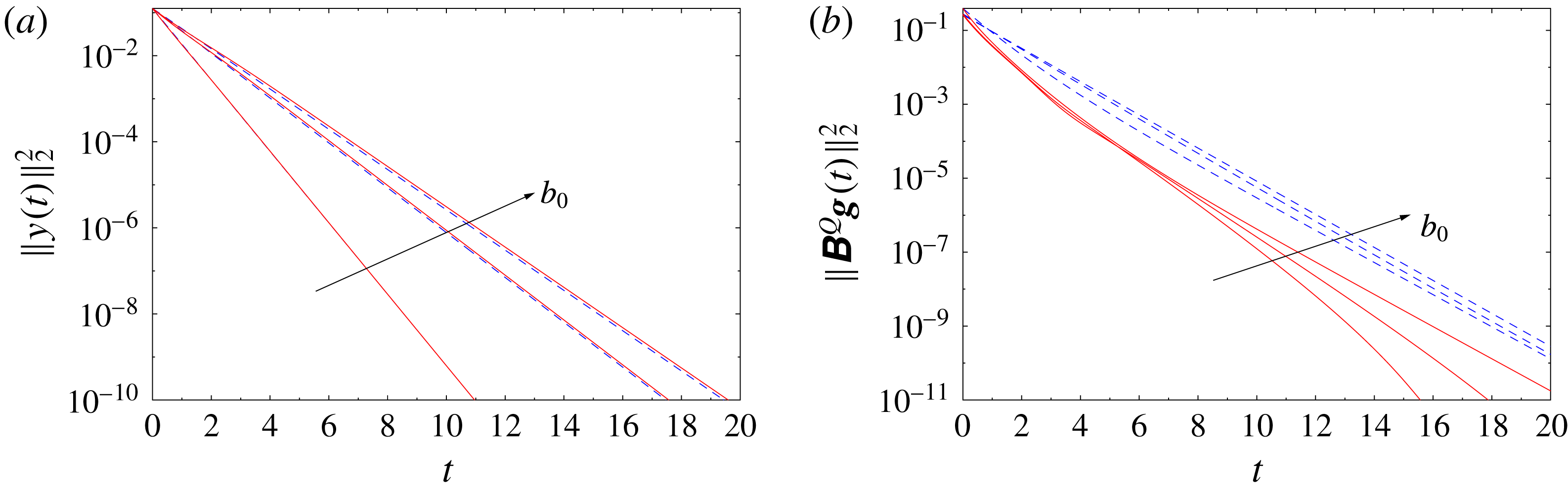
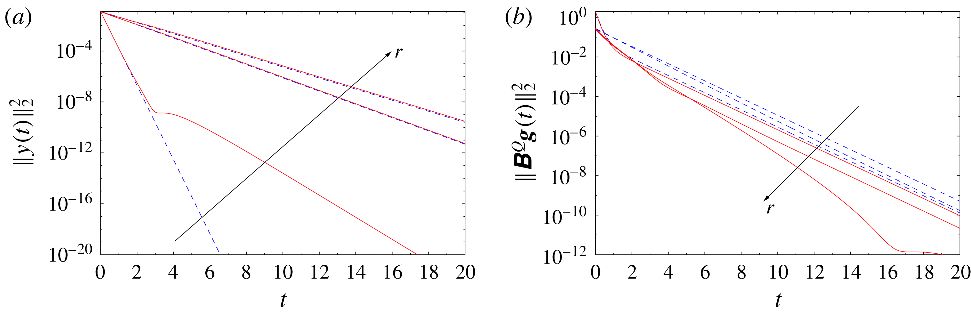
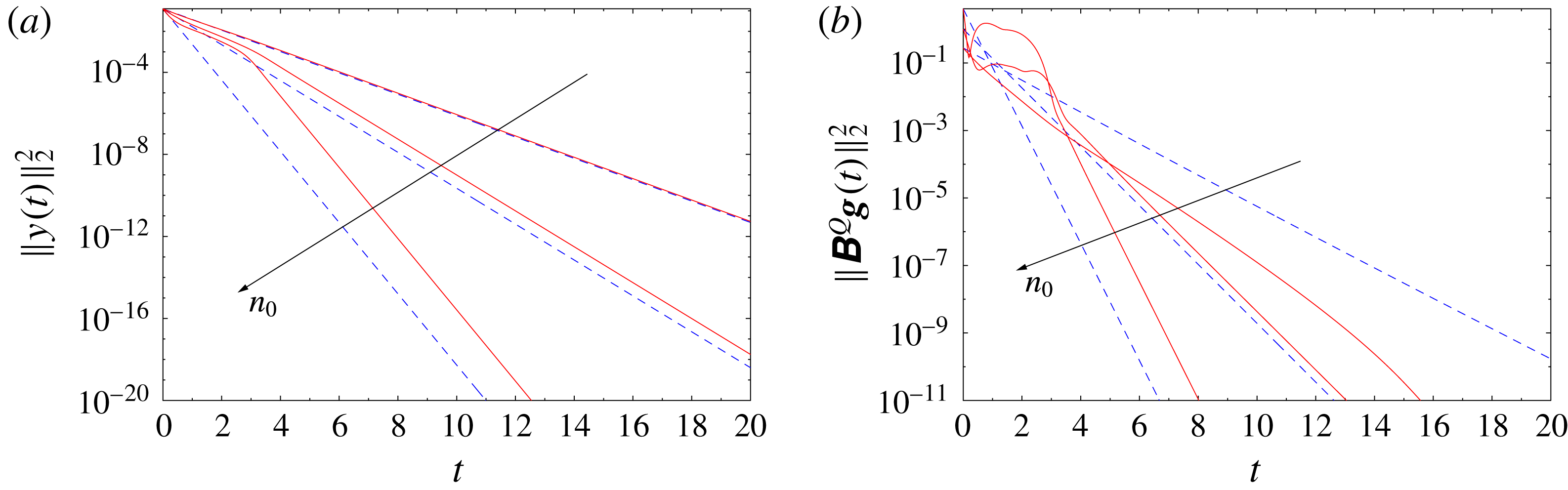
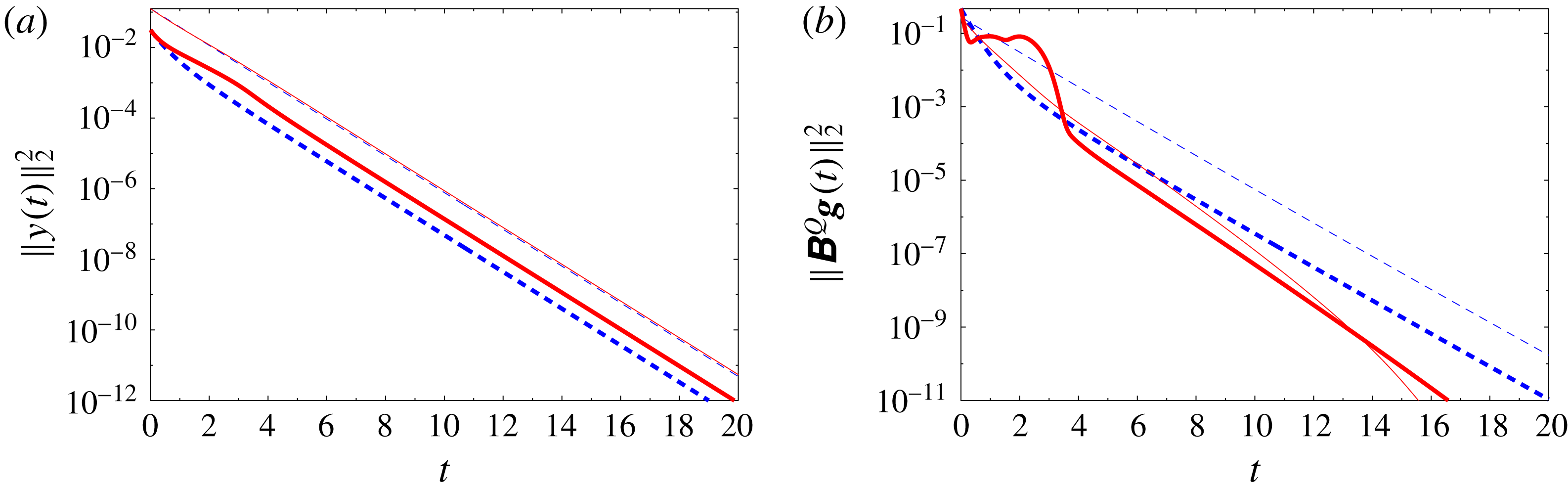
1 Introduction
Shear layers play a prominent role in fluid mechanics as canonical models of separated flows. Under typical conditions, they undergo the Kelvin–Helmholtz instability, during which the vorticity in the shear layer becomes concentrated in large vortex structures. Because of this universal feature, shear layers often serve as models for more complicated vortex-dominated flows arising in a broad range of applications. Their properties have already been investigated for a long time at the fundamental level from the experimental (Morris Reference Morris2011), theoretical (Maslowe Reference Maslowe1986) as well as the numerical standpoint (Comte, Lesieur & Lamballais Reference Comte, Lesieur and Lamballais1992). In addition to offering insights about transition to turbulence and the role played in this multiscale process by vortex structures, shear layers have also served as a playground for the application of various flow-control techniques aiming to stabilize the flow by preventing the growth of vortex structures. The literature on this topic is quite rich. As examples in this context, we mention the recent investigations by Pastoor et al. (Reference Pastoor, Henning, Noack, King and Tadmor2008), Wei & Rowley (Reference Wei and Rowley2009) and Kaiser et al. (Reference Kaiser, Noack, Cordier, Spohn, Segond, Abel, Daviller, Östh, Krajnović and Niven2014), which combine experimental, theoretical and numerical approaches. In the present study, we address the problem of stabilizing a shear layer at the fundamental level by combining a simple inviscid model of this phenomenon with methods of modern linear control theory.
Inviscid vortex models using singular vorticity distributions to represent flow fields have had a long and rich history in fluid mechanics. Our attention here will be focused exclusively on two-dimensional (2D) problems. The most common models of this type are point vortices, where the vorticity has the form of a collection of Dirac delta distributions with time-evolving locations governed by a system of nonlinear ordinary differential equations (ODEs) (Newton Reference Newton2001). While point vortices are typically (albeit not exclusively) employed to model compact vorticity distributions, continuous vorticity distributions, such as those arising in shear layers, are represented more accurately in terms of ‘vortex sheets’, where the singular vorticity distribution has the form of a continuous one-dimensional (1D) open or closed curve. In such models, the linear circulation density plays the role of ‘vorticity’ (which is not defined on the sheet) and can be interpreted in terms of the jump of the tangential velocity component across the sheet. The evolution of the sheet is governed by the Birkhoff–Rott equation, which is a singular integro-differential equation (Saffman Reference Saffman1992). Vortex sheets are subject to the Kelvin–Helmholtz instability: infinitesimal perturbations with wavenumber
 $n$
superimposed on a flat vortex sheet grow exponentially in time at a rate proportional to
 $|n|$
. Not only does this high-wavenumber instability give rise to ill-posedness in the sense of Hadamard, but, reinforced through nonlinear effects, it also causes the development of a finite-time curvature singularity in the sheet before large localized vortex structures can appear (Moore Reference Moore1979). As a result, computational studies involving the Birkhoff–Rott equation typically require some regularization in order to track its long-time evolution, usually in the form of the well-known ‘vortex-blob’ approach (Krasny Reference Krasny1986a
) or using the more recent Euler-alpha strategy (Holm, Nitsche & Putkaradze Reference Holm, Nitsche and Putkaradze2006). A generic feature characterizing the evolution of (regularized) inviscid vortex sheets is roll-up producing localized vortex spirals (Krasny Reference Krasny1986b
). It should be pointed out that the appearance of such rolling up vortex spirals is closely related to the emergence of the curvature singularity in the solutions of the regularized equation with complexified time (Sakajo Reference Sakajo2004a
). In addition, interaction of these vortex spirals leads to chaotic evolution (Moore Reference Moore2002) and complex mixing (Sakajo & Okamoto Reference Sakajo and Okamoto1998), marking the onset of turbulence in the shear layers. To summarize, it is fair to say that the Kelvin–Helmholtz instability acts as a key trigger for the emergence of turbulent mixing shear layers. Let us also note that there are many interesting mathematical questions concerning various properties of solutions to the Birkhoff–Rott equation, and we refer the reader to the collection edited by Caflisch (Reference Caflisch1989) and the monograph by Majda & Bertozzi (Reference Majda and Bertozzi2002) for further details on this topic. In the present study, we will focus on a flat periodic vortex sheet as an idealized model of a shear layer and will investigate how various forms of actuation combined with methods of the modern linear control theory can be used to overcome the Kelvin–Helmholtz instability and thus inhibit the emergence of turbulent shear layers. We will consider here an arguably more difficult case when there is no regularization in the Birkhoff–Rott equation.
The potential offered by the mathematical methods of control theory to solve various flow-control problems was recognized already in the 1990s. Two main classes of problems are of interest: open-loop, or off-line, control problems, where one seeks to optimize certain inputs such as, e.g., actuation through a particular form of boundary conditions, and closed-loop control problems, in which one typically attempts to stabilize the problem against disturbances through some form of state-based or output-based feedback. Problems in the first category usually have the form of partial differential equation (PDE)-constrained optimization and are often solved using variants of the adjoint-based method. On the other hand, problems in the second category require determination of suitable feedback operators (kernels), which in the linear setting is accomplished by solving some form of the operator Riccati equation. Since the seminal works of Bewley & Liu (Reference Bewley and Liu1998) and Bewley, Moin & Temam (Reference Bewley, Moin and Temam2001), both approaches have seen remarkable success in solving a range of diverse flow-control problems of both fundamental and applied significance. While a review of the corresponding literature is beyond the scope of this study, we refer the reader to the monograph by Gunzburger (Reference Gunzburger2003) and to the survey papers by Kim & Bewley (Reference Kim and Bewley2007), Bagheri et al. (Reference Bagheri, Henningson, Hoepffner and Schmid2009) and Brunton & Noack (Reference Brunton and Noack2015) for details. Another class of problems that relies on similar mathematical techniques is flow estimation based on incomplete and possibly noisy measurements. We remark that, in order to produce approaches applicable in real-life situations, flow-control techniques usually have to be combined with state estimation. Finally, due to their special mathematical structure, various vortex models offer particular opportunities for flow control, and progress along these lines was reviewed by Protas (Reference Protas2008).
The goal of the present study is first to provide a precise control-theoretic characterization of the inviscid vortex sheet model for various types of actuation. In this context, we demonstrate that the linearization of the Birkhoff–Rott equation around the flat-sheet configuration is in fact controllable when the actuation involves a sufficient number of point sinks/sources or point vortices located on each side of the sheet and at a certain distance from it. Then, we design a state-feedback stabilization strategy by synthesizing a linear-quadratic regulator (LQR) and assess its performance as a function of a number of different parameters in both the linear and nonlinear regimes. Due to certain peculiar properties of the Birkhoff–Rott equation and the considered form of actuation, computational solution of this problem requires a special approach relying on calculations performed with a very high arithmetic precision. Rather than design a control strategy applicable in actual experiments, our study aims to provide fundamental insights about opportunities and limitations inherent in feedback control of the Kelvin–Helmholtz instability. The structure of this paper is as follows. In the next section, we introduce the Birkhoff–Rott equation as a model of a shear layer and discuss its linearization as well as the form of the control actuation. In § 3, we present a control-theoretic characterization of this model and introduce the LQR stabilization strategy. Details concerning our numerical approach are discussed in § 4, whereas computational results are presented in § 5. Discussion of our findings and final conclusions are deferred to § 6. Some additional technical material is collected in two appendices.
2 Inviscid vortex sheets
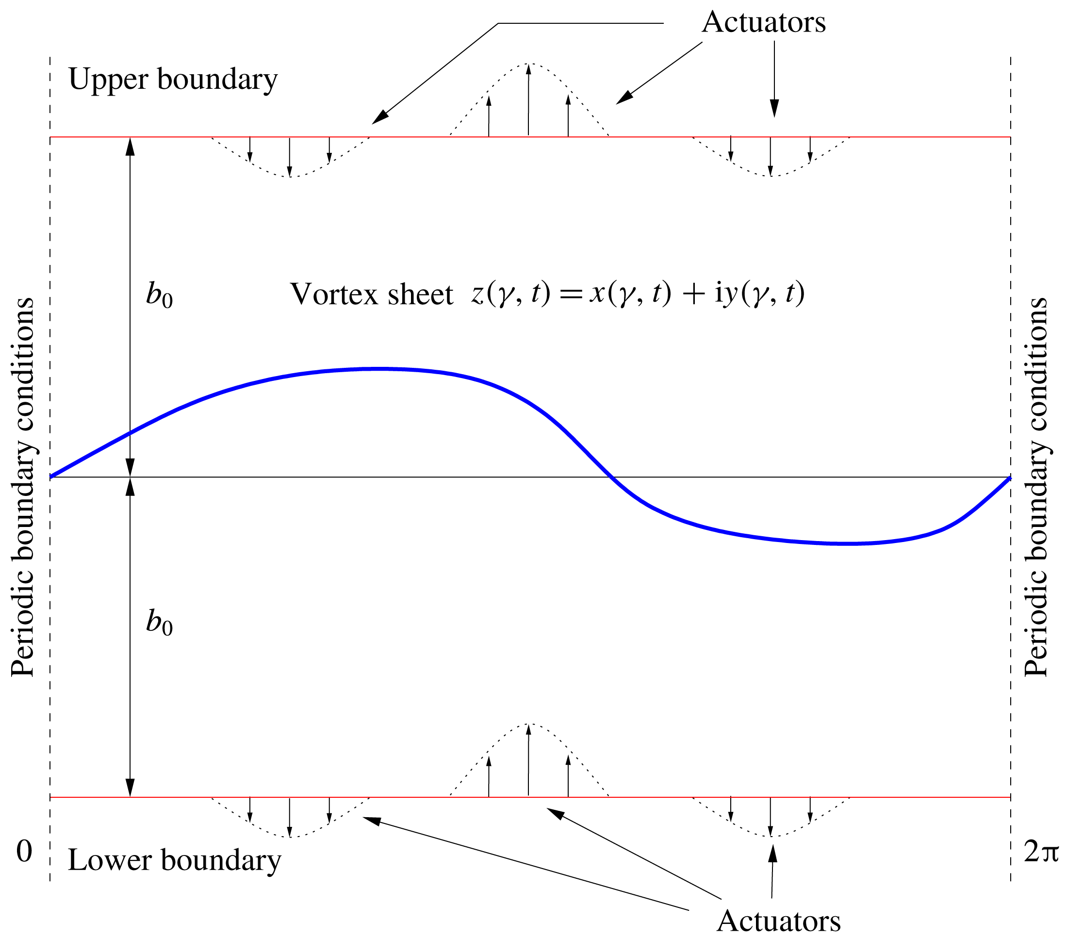
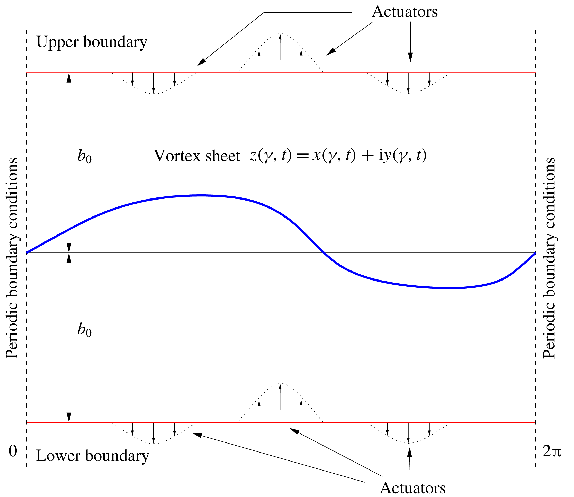
Schematic illustration of the problem set-up. The domain is
 $2\unicode[STIX]{x03C0}$
-periodic in the horizontal direction and the vortex sheet at time
 $t$
is represented by
 $z(\unicode[STIX]{x1D6FE},t)=x(\unicode[STIX]{x1D6FE},t)+\text{i}y(\unicode[STIX]{x1D6FE},t)$
, in which
 $\unicode[STIX]{x1D6FE}$
is a parameter varying along the sheet. An array of actuators is placed on a hypothetical boundary above and below the sheet.
In this section, we introduce a mathematical model for an inviscid vortex sheet in an unbounded domain, which, for simplicity, will be assumed to be periodic in the horizontal direction with a period of
 $2\unicode[STIX]{x03C0}$
. In § 2.2 below, we discuss how this model can be modified to account for the presence of actuators. We assume that the sheet has a constant intensity equal to one. As is common in the study of such problems (Saffman Reference Saffman1992), we will extensively use the complex representation of different quantities and will identify a point
 $(x,y)$
in the 2D space with
 $z=x+\text{i}y$
in the complex plane, where
 $\text{i}$
is the imaginary unit. Let then
 $z(\unicode[STIX]{x1D6FE},t)$
denote the position of a point on the sheet that corresponds to the circulation parameter
 $\unicode[STIX]{x1D6FE}\in [0,2\unicode[STIX]{x03C0}]$
and some time
 $t$
. The quantity
 $\unicode[STIX]{x1D6FE}$
represents a way of parameterizing the sheet, and for sheets of constant intensity is proportional to the arclength of the curve. Periodicity of the sheet then implies
 $$\begin{eqnarray}z(\unicode[STIX]{x1D6FE}+2\unicode[STIX]{x03C0},t)=z(\unicode[STIX]{x1D6FE},t)+2\unicode[STIX]{x03C0},\quad \unicode[STIX]{x1D6FE}\in [0,2\unicode[STIX]{x03C0}].\end{eqnarray}$$
The flow set-up is shown schematically in figure 1. Under the assumptions of periodicity and constant unit strength, the Birkhoff–Rott equation describing the evolution of the vortex sheet takes the form
 $$\begin{eqnarray}\frac{\unicode[STIX]{x2202}z^{\ast }}{\unicode[STIX]{x2202}t}(\unicode[STIX]{x1D6FE},t)=V(z(\unicode[STIX]{x1D6FE},t))\,\equiv \,{\displaystyle \frac{1}{4\unicode[STIX]{x03C0}\text{i}}}\text{pv}\int _{0}^{2\unicode[STIX]{x03C0}}\cot \left({\displaystyle \frac{z(\unicode[STIX]{x1D6FE},t)-z(\unicode[STIX]{x1D6FE}^{\prime },t)}{2}}\right)\,\text{d}\unicode[STIX]{x1D6FE}^{\prime },\end{eqnarray}$$
where
 $z^{\ast }$
denotes the complex conjugate of
 $z$
, the integral on the right-hand side is understood in Cauchy’s principal-value sense and
 $V(z)=(u-\text{i}v)(z)$
represents the complex velocity at the point
 $z$
, with
 $u$
and
 $v$
the horizontal and vertical velocity components respectively. Equation (2.2) is complemented with a suitable initial condition
 $z(\unicode[STIX]{x1D6FE},0)=z_{0}(\unicode[STIX]{x1D6FE})$
,
 $\unicode[STIX]{x1D6FE}\in [0,2\unicode[STIX]{x03C0}]$
. As can be readily verified, equation (2.2) admits an equilibrium solution (a fixed point)
 $\tilde{z}(\unicode[STIX]{x1D6FE},t)=\unicode[STIX]{x1D6FE}$
for
 $\unicode[STIX]{x1D6FE}\in [0,2\unicode[STIX]{x03C0}]$
, i.e.
 $(\unicode[STIX]{x2202}/\unicode[STIX]{x2202}t)\tilde{z}^{\ast }(\unicode[STIX]{x1D6FE},t)=0$
, which corresponds to a flat (undeformed) sheet. The linear stability of this equilibrium configuration will be discussed below.
2.1 Kelvin–Helmholtz instability
We now characterize the Kelvin–Helmholtz instability undergone by the flat-sheet equilibrium configuration. This will be done by performing a linear-stability analysis of the Birkhoff–Rott equation in the neighbourhood of the fixed point
 $\tilde{z}$
. Following the approach of Sakajo & Okamoto (Reference Sakajo and Okamoto1996), see also Kiya & Arie (Reference Kiya and Arie1979), suppose that we perturb this equilibrium state infinitesimally as
 $$\begin{eqnarray}z(\unicode[STIX]{x1D6FE},t)=\unicode[STIX]{x1D6FE}+\unicode[STIX]{x1D700}\unicode[STIX]{x1D701}(\unicode[STIX]{x1D6FE},t),\end{eqnarray}$$
for
 $0<\unicode[STIX]{x1D700}\ll 1$
. Here,
 $\unicode[STIX]{x1D701}(\unicode[STIX]{x1D6FE},t)$
is a perturbation represented in the periodic setting, cf. (2.1), as
 $$\begin{eqnarray}\unicode[STIX]{x1D701}(\unicode[STIX]{x1D6FE},t)=\mathop{\sum }_{n=-\infty }^{\infty }\widehat{\unicode[STIX]{x1D701}}_{n}(t)\text{e}^{\text{i}n\unicode[STIX]{x1D6FE}},\end{eqnarray}$$
in which
 $\widehat{\unicode[STIX]{x1D701}}_{n}\in \mathbb{C}$
,
 $n\in \mathbb{Z}$
, are the Fourier coefficients. Then, we obtain the linearized equation for
 $\unicode[STIX]{x1D701}(\unicode[STIX]{x1D6FE},t)$
as follows:
 $$\begin{eqnarray}\displaystyle {\displaystyle \frac{\unicode[STIX]{x2202}\unicode[STIX]{x1D701}^{\ast }}{\unicode[STIX]{x2202}t}}(\unicode[STIX]{x1D6FE},t) & = & \displaystyle -{\displaystyle \frac{1}{8\unicode[STIX]{x03C0}\text{i}}}\text{pv}\int _{0}^{2\unicode[STIX]{x03C0}}{\displaystyle \frac{\unicode[STIX]{x1D701}(\unicode[STIX]{x1D6FE},t)-\unicode[STIX]{x1D701}(\unicode[STIX]{x1D6FE}^{\prime },t)}{\sin ^{2}\left({\displaystyle \frac{\unicode[STIX]{x1D6FE}-\unicode[STIX]{x1D6FE}^{\prime }}{2}}\right)}}\,\text{d}\unicode[STIX]{x1D6FE}^{\prime }\nonumber\\ \displaystyle & = & \displaystyle \mathop{\sum }_{n=-\infty }^{\infty }\widehat{\unicode[STIX]{x1D701}}_{n}(t)\text{e}^{\text{i}n\unicode[STIX]{x1D6FE}}\left[-{\displaystyle \frac{1}{8\unicode[STIX]{x03C0}\text{i}}}\text{pv}\int _{0}^{2\unicode[STIX]{x03C0}}{\displaystyle \frac{1-\text{e}^{-\text{i}n\unicode[STIX]{x1D6FE}^{\prime }}}{\sin ^{2}\left({\displaystyle \frac{\unicode[STIX]{x1D6FE}^{\prime }}{2}}\right)}}\,\text{d}\unicode[STIX]{x1D6FE}^{\prime }\right]\nonumber\\ \displaystyle & = & \displaystyle \mathop{\sum }_{n=-\infty }^{\infty }\widehat{\unicode[STIX]{x1D701}}_{n}(t)\text{e}^{\text{i}n\unicode[STIX]{x1D6FE}}\left[-{\displaystyle \frac{1}{4\text{i}}}\text{pv}\int _{0}^{1}{\displaystyle \frac{1-\cos (2\unicode[STIX]{x03C0}n\unicode[STIX]{x1D70F})-\text{i}\sin (2\unicode[STIX]{x03C0}n\unicode[STIX]{x1D70F})}{\sin ^{2}(\unicode[STIX]{x03C0}\unicode[STIX]{x1D70F})}}\,\text{d}\unicode[STIX]{x1D70F}\right]\nonumber\\ \displaystyle & = & \displaystyle -{\displaystyle \frac{1}{2\text{i}}}\mathop{\sum }_{n=1}^{\infty }n\,\widehat{\unicode[STIX]{x1D701}}_{n}(t)\text{e}^{\text{i}n\unicode[STIX]{x1D6FE}}-{\displaystyle \frac{1}{2\text{i}}}\mathop{\sum }_{n=1}^{\infty }n\,\widehat{\unicode[STIX]{x1D701}}_{-n}(t)\text{e}^{-\text{i}n\unicode[STIX]{x1D6FE}}.\end{eqnarray}$$
Since
 $$\begin{eqnarray}{\displaystyle \frac{\unicode[STIX]{x2202}\unicode[STIX]{x1D701}^{\ast }}{\unicode[STIX]{x2202}t}}=\mathop{\sum }_{n=-\infty }^{\infty }{\displaystyle \frac{\text{d}\widehat{\unicode[STIX]{x1D701}}_{n}^{\ast }}{\text{d}t}}\text{e}^{-\text{i}n\unicode[STIX]{x1D6FE}}=\mathop{\sum }_{n=1}^{\infty }{\displaystyle \frac{\text{d}\widehat{\unicode[STIX]{x1D701}}_{n}^{\ast }}{\text{d}t}}\text{e}^{-\text{i}n\unicode[STIX]{x1D6FE}}+\mathop{\sum }_{n=1}^{\infty }{\displaystyle \frac{\text{d}\widehat{\unicode[STIX]{x1D701}}_{-n}^{\ast }}{\text{d}t}}\text{e}^{\text{i}n\unicode[STIX]{x1D6FE}}+{\displaystyle \frac{\text{d}\widehat{\unicode[STIX]{x1D701}}_{0}}{\text{d}t}},\end{eqnarray}$$
equating coefficients of the Fourier components in (2.5) and (2.6) corresponding to different wavenumbers
 $n$
, we obtain linearized equations for the coefficients
 $\widehat{\unicode[STIX]{x1D701}}_{n}$
in a block-diagonal form,
 $$\begin{eqnarray}\displaystyle {\displaystyle \frac{\text{d}\widehat{\unicode[STIX]{x1D701}}_{-n}^{\ast }}{\text{d}t}} & = & \displaystyle \phantom{-}{\displaystyle \frac{\text{i}n}{2}}\widehat{\unicode[STIX]{x1D701}}_{n},\end{eqnarray}$$
 $$\begin{eqnarray}\displaystyle {\displaystyle \frac{\text{d}\widehat{\unicode[STIX]{x1D701}}_{n}}{\text{d}t}} & = & \displaystyle -{\displaystyle \frac{\text{i}n}{2}}\widehat{\unicode[STIX]{x1D701}}_{-n}^{\ast },\end{eqnarray}$$
 $$\begin{eqnarray}\displaystyle {\displaystyle \frac{\text{d}\widehat{\unicode[STIX]{x1D701}}_{0}}{\text{d}t}} & = & \displaystyle \phantom{-}0,\end{eqnarray}$$
 $n\geqslant 1$
. This step thus allows us to convert the original continuous PDE problem to an infinite system of ODEs. Since this latter system has a block-diagonal structure, key insights about the infinite-dimensional problem can be obtained by analysing just a single block, independently from all other blocks. The eigenvalues corresponding to each diagonal block with
 $n\geqslant 1$
, cf. (2.7a
)–(2.7b
), are
 $\unicode[STIX]{x1D706}_{n}=\pm n/2$
. Since the system must be recast in a purely real form for our subsequent analysis of its controllability in § 3, we need to rewrite the linearized equations (2.7a
) and (2.7b
) in terms of the real and imaginary parts of the Fourier coefficients
 $\widehat{\unicode[STIX]{x1D701}}_{n}=\unicode[STIX]{x1D6FC}_{n}+\text{i}\unicode[STIX]{x1D6FD}_{n}$
and
 $\widehat{\unicode[STIX]{x1D701}}_{-n}=\unicode[STIX]{x1D6FC}_{-n}+\text{i}\unicode[STIX]{x1D6FD}_{-n}$
as
 $$\begin{eqnarray}\displaystyle {\displaystyle \frac{\text{d}}{\text{d}t}}(\unicode[STIX]{x1D6FC}_{-n}-\text{i}\unicode[STIX]{x1D6FD}_{-n}) & = & \displaystyle {\displaystyle \frac{\text{i}n}{2}}(\unicode[STIX]{x1D6FC}_{n}+\text{i}\unicode[STIX]{x1D6FD}_{n})=-\text{i}B_{-n}(\unicode[STIX]{x1D6FC}_{n}+\text{i}\unicode[STIX]{x1D6FD}_{n}),\end{eqnarray}$$
 $$\begin{eqnarray}\displaystyle {\displaystyle \frac{\text{d}}{\text{d}t}}(\unicode[STIX]{x1D6FC}_{n}+\text{i}\unicode[STIX]{x1D6FD}_{n}) & = & \displaystyle -{\displaystyle \frac{\text{i}n}{2}}(\unicode[STIX]{x1D6FC}_{-n}-\text{i}\unicode[STIX]{x1D6FD}_{-n})=\text{i}B_{n}(\unicode[STIX]{x1D6FC}_{-n}-\text{i}\unicode[STIX]{x1D6FD}_{-n}),\end{eqnarray}$$
 $$\begin{eqnarray}B_{-n}=B_{n}=-{\displaystyle \frac{n}{2}},\quad n\geqslant 1.\end{eqnarray}$$
Hereafter, the real and imaginary parts of the Fourier coefficients will serve as our state variables. By defining the vector of the state variables associated with the wavenumber
 $n$
as
 $\boldsymbol{X}_{n}=[\unicode[STIX]{x1D6FC}_{-n}~\unicode[STIX]{x1D6FD}_{n}~\unicode[STIX]{x1D6FD}_{-n}~\unicode[STIX]{x1D6FC}_{n}]^{\text{T}}$
, relations (2.8) can be recast in the following form:
 $$\begin{eqnarray}{\displaystyle \frac{\text{d}}{\text{d}t}}\left[\begin{array}{@{}c@{}}\unicode[STIX]{x1D6FC}_{-n}\\ \unicode[STIX]{x1D6FD}_{n}\\ \unicode[STIX]{x1D6FD}_{-n}\\ \unicode[STIX]{x1D6FC}_{n}\end{array}\right]=-{\displaystyle \frac{n}{2}}\left[\begin{array}{@{}cccc@{}}0 & 1 & 0 & 0\\ 1 & 0 & 0 & 0\\ 0 & 0 & 0 & 1\\ 0 & 0 & 1 & 0\end{array}\right]\left[\begin{array}{@{}c@{}}\unicode[STIX]{x1D6FC}_{-n}\\ \unicode[STIX]{x1D6FD}_{n}\\ \unicode[STIX]{x1D6FD}_{-n}\\ \unicode[STIX]{x1D6FC}_{n}\end{array}\right],\end{eqnarray}$$
which can be rewritten more compactly as
 $$\begin{eqnarray}{\displaystyle \frac{\text{d}\boldsymbol{X}_{n}}{\text{d}t}}=-{\displaystyle \frac{n}{2}}\unicode[STIX]{x1D63C}_{0}\boldsymbol{X}_{n}=\unicode[STIX]{x1D63C}_{n}\boldsymbol{X}_{n},\quad n\geqslant 1,\end{eqnarray}$$
where
 $\unicode[STIX]{x1D63C}_{n}=-(n/2)\unicode[STIX]{x1D63C}_{0}$
and
 $$\begin{eqnarray}\unicode[STIX]{x1D63C}_{0}=\left[\begin{array}{@{}cc@{}}\unicode[STIX]{x1D63E} & 0\\ 0 & \unicode[STIX]{x1D63E}\end{array}\right],\quad \text{with }\unicode[STIX]{x1D63E}=\left[\begin{array}{@{}cc@{}}0 & 1\\ 1 & 0\end{array}\right].\end{eqnarray}$$
It is well known that the stability properties of linear systems with block-diagonal structure are determined by the eigenvalues and eigenvectors of the individual blocks. We thus observe that, for each wavenumber
 $n\geqslant 1$
, the evolution described by system (2.11) is characterized by two invariant subspaces spanned by the vectors
 $[\unicode[STIX]{x1D6FC}_{-n}~\unicode[STIX]{x1D6FD}_{n}~0~0]^{\text{T}}$
and
 $[0~0~\unicode[STIX]{x1D6FD}_{-n}~\unicode[STIX]{x1D6FC}_{n}]^{\text{T}}$
, which are orthogonal to each other. Each of these subspaces contains a growing and a decaying mode, with the growth rates given by the eigenvalues
 $\unicode[STIX]{x1D706}_{n}^{+}=n/2$
and
 $\unicode[STIX]{x1D706}_{n}^{-}=-n/2$
. Therefore, for each wavenumber
 $n\geqslant 1$
, we have two unstable modes proportional to
 $$\begin{eqnarray}\displaystyle \widehat{\unicode[STIX]{x1D743}}_{1} & = & \displaystyle [-1~1~0~0]^{\text{T}},\end{eqnarray}$$
 $$\begin{eqnarray}\displaystyle \widehat{\unicode[STIX]{x1D743}}_{2} & = & \displaystyle [0~0~-1~1]^{\text{T}}\end{eqnarray}$$
 $$\begin{eqnarray}\displaystyle \widehat{\unicode[STIX]{x1D743}}_{3} & = & \displaystyle [1~1~0~0]^{\text{T}},\end{eqnarray}$$
 $$\begin{eqnarray}\displaystyle \widehat{\unicode[STIX]{x1D743}}_{4} & = & \displaystyle [0~0~1~1]^{\text{T}},\end{eqnarray}$$
 $\widehat{\unicode[STIX]{x1D743}}_{1},\widehat{\unicode[STIX]{x1D743}}_{2},\widehat{\unicode[STIX]{x1D743}}_{3},\widehat{\unicode[STIX]{x1D743}}_{4}$
are the (right) eigenvectors of the matrix
 $\unicode[STIX]{x1D63C}_{n}$
. We note that these eigenvectors are mutually orthogonal and that the matrices
 $\unicode[STIX]{x1D63C}_{n}$
,
 $n\geqslant 1$
, are normal. In the light of ansatz (2.4), the eigenvectors
 $\widehat{\unicode[STIX]{x1D743}}_{1},\widehat{\unicode[STIX]{x1D743}}_{2},\widehat{\unicode[STIX]{x1D743}}_{3},\widehat{\unicode[STIX]{x1D743}}_{4}$
take the following forms in the ‘physical’ space as functions of the coordinate
 $\unicode[STIX]{x1D6FE}$
:
 $$\begin{eqnarray}\displaystyle \unicode[STIX]{x1D709}_{1}(\unicode[STIX]{x1D6FE}) & = & \displaystyle \unicode[STIX]{x1D713}_{n}(\unicode[STIX]{x1D6FE})(1-\text{i}),\end{eqnarray}$$
 $$\begin{eqnarray}\displaystyle \unicode[STIX]{x1D709}_{2}(\unicode[STIX]{x1D6FE}) & = & \displaystyle \unicode[STIX]{x1D719}_{n}(\unicode[STIX]{x1D6FE})(1-\text{i}),\end{eqnarray}$$
 $$\begin{eqnarray}\displaystyle \unicode[STIX]{x1D709}_{3}(\unicode[STIX]{x1D6FE}) & = & \displaystyle \unicode[STIX]{x1D719}_{n}(\unicode[STIX]{x1D6FE})(1+\text{i}),\end{eqnarray}$$
 $$\begin{eqnarray}\displaystyle \unicode[STIX]{x1D709}_{4}(\unicode[STIX]{x1D6FE}) & = & \displaystyle \unicode[STIX]{x1D713}_{n}(\unicode[STIX]{x1D6FE})(1+\text{i}),\end{eqnarray}$$
 $$\begin{eqnarray}\unicode[STIX]{x1D719}_{n}(\unicode[STIX]{x1D6FE})=\cos (n\unicode[STIX]{x1D6FE})-\sin (n\unicode[STIX]{x1D6FE}),\quad \unicode[STIX]{x1D713}_{n}(\unicode[STIX]{x1D6FE})=\cos (n\unicode[STIX]{x1D6FE})+\sin (n\unicode[STIX]{x1D6FE}).\end{eqnarray}$$
These functions satisfy the relation
 $\unicode[STIX]{x1D719}_{n}(\unicode[STIX]{x1D6FE})=\unicode[STIX]{x1D713}_{n}(2\unicode[STIX]{x03C0}-\unicode[STIX]{x1D6FE})$
, which implies that the pairs of unstable and stable eigenvectors, respectively
 $\unicode[STIX]{x1D709}_{1/2}$
and
 $\unicode[STIX]{x1D709}_{3/4}$
, have the same form, but different phases. The equilibrium configurations
 $\tilde{z}$
perturbed with the unstable eigenvectors
 $\unicode[STIX]{x1D709}_{1}$
and
 $\unicode[STIX]{x1D709}_{2}$
defined for a single wavenumber
 $n=1$
, cf. (2.3), and with perturbations obtained by superposing components
 $\unicode[STIX]{x1D709}_{1}$
and
 $\unicode[STIX]{x1D709}_{2}$
with different wavenumbers
 $n=1,2,3,4$
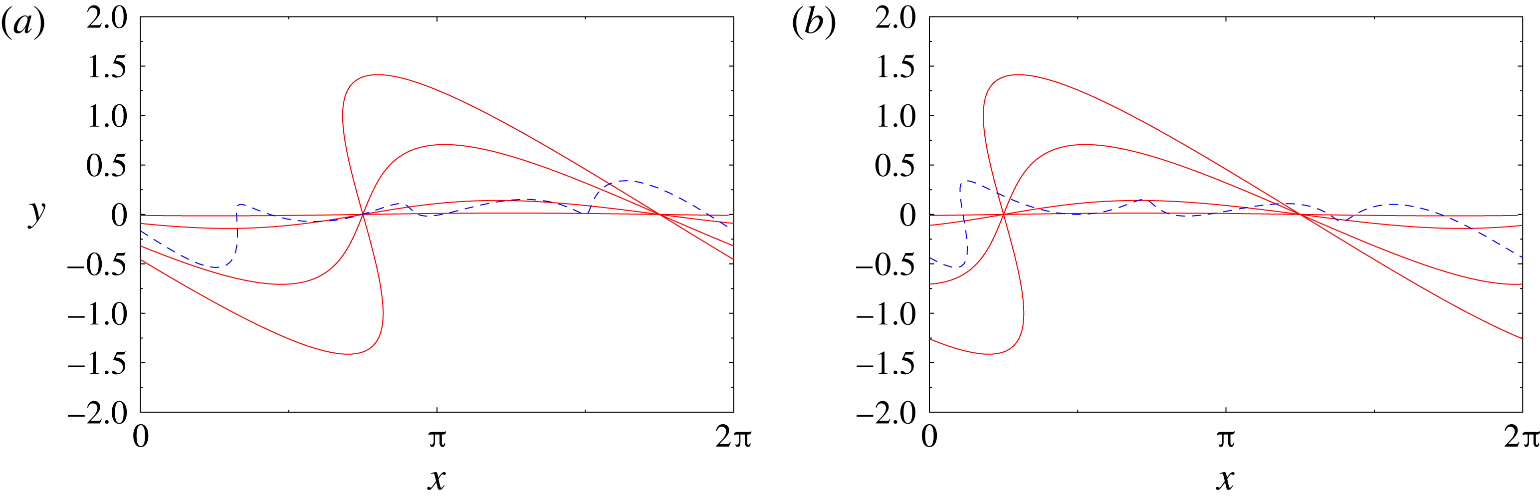
are shown in the ‘physical’ space in figure 2. Noting that
 $$\begin{eqnarray}\cos (n\unicode[STIX]{x1D6FE})={\textstyle \frac{1}{2}}[\unicode[STIX]{x1D713}_{n}(\unicode[STIX]{x1D6FE})+\unicode[STIX]{x1D719}_{n}(\unicode[STIX]{x1D6FE})],\quad \sin (n\unicode[STIX]{x1D6FE})={\textstyle \frac{1}{2}}[\unicode[STIX]{x1D713}_{n}(\unicode[STIX]{x1D6FE})-\unicode[STIX]{x1D719}_{n}(\unicode[STIX]{x1D6FE})],\end{eqnarray}$$
we conclude that every perturbation
 $\widehat{\unicode[STIX]{x1D701}}_{n}(t)\text{e}^{\text{i}n\unicode[STIX]{x1D6FE}}$
with the wavenumber
 $n$
can be uniquely decomposed in terms of the four eigenvectors (2.15a
)–(2.15d
). The above observations will simplify our analysis of the control-theoretic properties of the system presented in § 3.
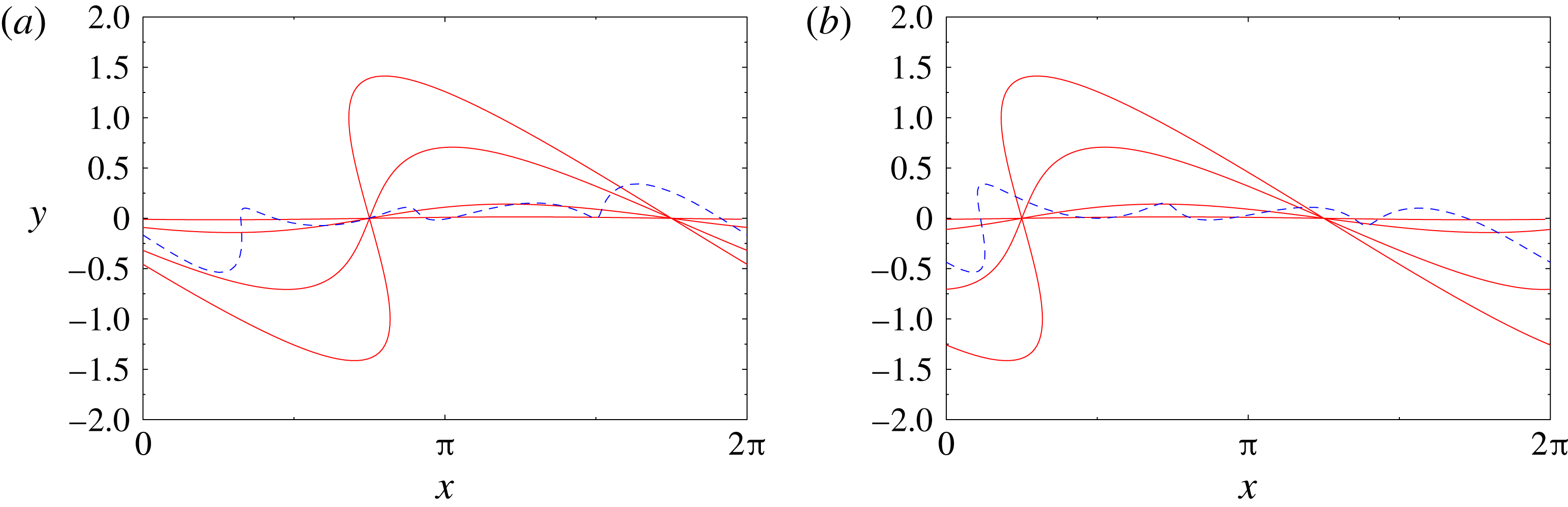
Equilibrium configuration
 $\tilde{z}$
perturbed with the unstable eigenvectors (a)
 $\unicode[STIX]{x1D709}_{1}$
and (b)
 $\unicode[STIX]{x1D709}_{2}$
for (red solid lines)
 $n=1$
and
 $\unicode[STIX]{x1D700}=0.01$
,
 $0.1$
,
 $0.5$
and
 $1.0$
, cf. (2.3); the blue dashed lines represent equilibrium configurations with perturbations obtained by superposing components
 $\unicode[STIX]{x1D709}_{1}$
and
 $\unicode[STIX]{x1D709}_{2}$
with different wavenumbers
 $n=1,2,3,4$
and the same value
 $\unicode[STIX]{x1D700}=0.1$
.
We thus conclude that the linearization of the Birkhoff–Rott equation in the neighbourhood of the flat-sheet equilibrium
 $\tilde{z}$
is characterized by a discrete spectrum of orthogonal unstable modes whose growth rates increase in proportion to the wavenumber
 $n$
. We add that the regularization approaches mentioned in § 1 would strongly suppress this instability at higher wavenumbers by introducing an upper bound on the growth rates (Holm et al.
Reference Holm, Nitsche and Putkaradze2006).
2.2 Actuation
The form of actuation used in our study is an idealized representation of the forcing typically employed in actual experiments involving control of shear layers, i.e. distributed blowing and suction, microjets, etc. To account for such actuation, we modify the model introduced above by incorporating two hypothetical horizontal solid boundaries located a certain distance
 $b_{0}>0$
above and below the sheet in its undeformed configuration (figure 1). We then suppose that actuation is produced by arrays of point sink/sources or point vortices located at each of the boundaries. We note that in the absence of actuation and when the vortex sheet is in its equilibrium (undeformed) configuration
 $\tilde{z}$
, the corresponding flow induced by the sheet is everywhere parallel to the boundaries; hence, it satisfies the no-through-flow boundary condition required by the Euler equation. On the other hand, when the sheet is deformed as in (2.3), a small wall-normal velocity, of order
 $O(\unicode[STIX]{x1D700}/b_{0})$
, is induced on the boundaries. In principle, it could be eliminated by including a suitable potential velocity field in the model (2.2). However, in order to keep our model analytically tractable, we neglect this effect.
Each of the boundaries contains an array of
 $N_{c}$
point sinks/sources or point vortices, so that the total number of actuators is
 $2N_{c}$
. Their locations will be denoted
 $w_{k}=a_{k}+\text{i}b_{k}$
, where
 $a_{k},b_{k}\in \mathbb{R}$
,
 $k=1,\ldots ,2N_{c}$
, with odd (even) indices
 $k$
corresponding to actuators above (below) the sheet. Since the two boundaries are located at the same distance
 $b_{0}$
from the sheet, we have
 $b_{1}=b_{3}=\cdots =b_{2N_{c}-1}=b_{0}$
and
 $b_{2}=b_{4}=\cdots =b_{2N_{c}}=-b_{0}$
. Since each of the arrays consists of actuators equispaced in the horizontal direction, we also have
 $a_{2k+1}=a_{1}+2\unicode[STIX]{x03C0}k/N_{c}$
and
 $a_{2k+2}=a_{2}+2\unicode[STIX]{x03C0}k/N_{c}$
,
 $k=1,\ldots ,N_{c}-1$
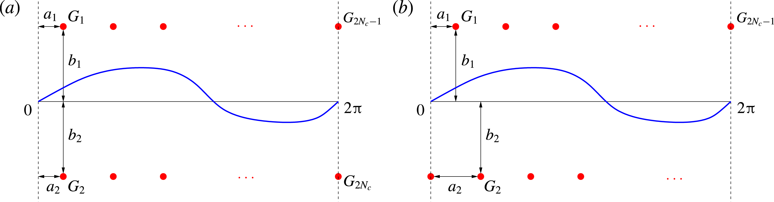
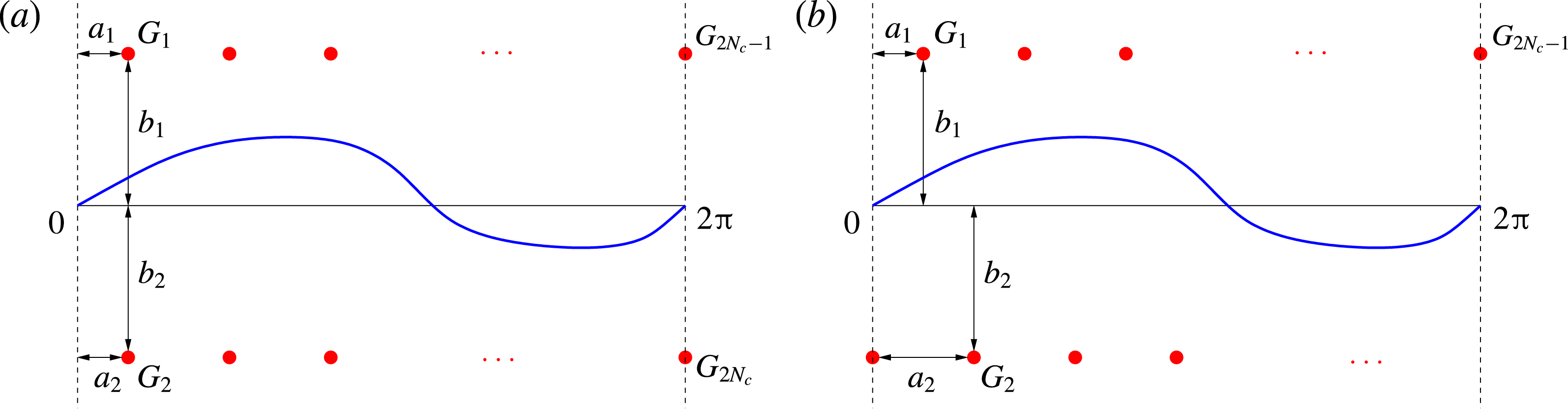
. As regards the relative location of the actuators in the two arrays, we will consider two arrangements: aligned (with
 $a_{1}=a_{2}$
; see figure 3
a) and staggered (with
 $|a_{2}-a_{1}|=\unicode[STIX]{x03C0}/N_{c}$
; see figure 3
b). We note that since, due to periodicity, the system is invariant with respect to translation in the
 $x$
direction, the actual values of
 $a_{1}$
and
 $a_{2}$
are unimportant and what matters is only the difference
 $|a_{2}-a_{1}|$
. The velocity induced at a certain point
 $\unicode[STIX]{x1D712}\in \mathbb{C}$
by an individual, say
 $k$
th, actuator is given by the expression
 $(G_{k}/(4\unicode[STIX]{x03C0}\text{i}))\cot ((\unicode[STIX]{x1D712}-w_{k})/2)$
,
 $\unicode[STIX]{x1D712}\neq w_{k}$
, where
 $G_{k}\in \mathbb{C}$
is the strength of the actuator. It can be given either in terms of the intensity
 $Q_{k}\in \mathbb{R}$
of the point sink/source, i.e.
 $G_{k}=\text{i}Q_{k}$
, or in terms of the circulation
 $\unicode[STIX]{x1D6E4}_{k}\in \mathbb{R}$
of the point vortex, i.e.
 $G_{k}=\unicode[STIX]{x1D6E4}_{k}$
. As regards the two forms of the actuation, we remark that point sinks/sources, which can be viewed as idealized models for localized blowing and suction, generate velocity fields that are radial with respect to the actuator location
 $w_{k}$
. Therefore, such a velocity field does not violate the no-through-flow boundary condition on the horizontal wall on which the actuator is mounted (this boundary condition is in fact violated by the velocity field induced by the actuators located at the opposite boundary, regardless of their form, but this effect is of order
 $O(b_{0}^{-1})$
and can therefore be neglected unless the actuators are placed close to the vortex sheet). On the other hand, point vortices, which can be viewed as idealized models for localized vorticity generation, induce velocity fields with closed streamlines concentric around the actuator location
 $w_{k}$
. Therefore, this velocity field will significantly violate the no-through-flow condition on the horizontal boundary in the neighbourhood of the actuator location
 $w_{k}$
. For this reason, in this study, we will primarily focus on point sinks/sources used as actuators and, for the sake of completeness, we will also briefly consider actuation with point vortices.
The time-dependent sink/source intensities and vortex circulations,
 $Q_{k}=Q_{k}(t)$
and
 $\unicode[STIX]{x1D6E4}_{k}=\unicode[STIX]{x1D6E4}_{k}(t)$
, will be determined by a feedback control algorithm which will be designed in § 3.3. In the presence of such actuation, the Birkhoff–Rott equation (2.2) takes the following form:
 $$\begin{eqnarray}{\displaystyle \frac{\unicode[STIX]{x2202}z^{\ast }}{\unicode[STIX]{x2202}t}}(\unicode[STIX]{x1D6FE},t)={\displaystyle \frac{1}{4\unicode[STIX]{x03C0}\text{i}}}\text{pv}\int _{0}^{2\unicode[STIX]{x03C0}}\cot \left({\displaystyle \frac{z(\unicode[STIX]{x1D6FE},t)-z(\unicode[STIX]{x1D6FE}^{\prime },t)}{2}}\right)\,\text{d}\unicode[STIX]{x1D6FE}^{\prime }+\mathop{\sum }_{k=1}^{2N_{c}}{\displaystyle \frac{G_{k}}{4\unicode[STIX]{x03C0}\text{i}}}\cot \left({\displaystyle \frac{z(\unicode[STIX]{x1D6FE},t)-w_{k}}{2}}\right).\end{eqnarray}$$
Schematic representations of the actuation set-up with (a) an aligned and (b) a staggered arrangement of point vortices or sinks/sources (denoted by red solid circles). The undeformed and perturbed vortex sheets are represented with thin black and thick blue lines respectively.
The actuator strengths
 $G_{1}(t),\ldots ,G_{2N_{c}}(t)$
are not all independent. When point sinks/sources are used, mass must be conserved in time not only globally but also independently in each of the subdomains above and below the sheet, as otherwise there would be a net mass flux across the sheet, which is undesirable. Consequently, the actuation must act such that the net mass flux produced by the point sinks/sources both above and below the sheet is zero. Likewise, when point vortices are used, their total circulation must also be conserved in order to satisfy Kelvin’s theorem. Moreover, to ensure that such actuation does not generate a net flow in the horizontal direction, the circulations of the point vortices above and below the sheet must independently add up to zero. These constraints can be expressed as the following relations:
 $$\begin{eqnarray}\displaystyle G_{1}(t)+G_{3}(t)+\cdots +G_{2Nc-1}(t) & = & \displaystyle 0,\end{eqnarray}$$
 $$\begin{eqnarray}\displaystyle G_{2}(t)+G_{4}(t)+\cdots +G_{2Nc}(t) & = & \displaystyle 0,\end{eqnarray}$$
To summarize, the choices determining the actuation set-up are as follows: (i) the number
 $N_{c}$
of actuator pairs, (ii) aligned versus staggered arrangement of the actuators and (iii) the parameter
 $b_{0}$
representing the distance between the actuators and the undeformed vortex sheet.
3 Control-oriented characterization of the system
In this section, we first characterize the input-to-state properties of the linearized system (2.5) from the control-theoretic point of view. This will allow us to assess whether the Kelvin–Helmholtz instability analysed in § 2.1 can be stabilized using a linear state-feedback control approach based on the actuation described in § 2.2. Then, based on these results, we will design an LQR stabilization approach.
From the discussion at the end of § 2.2, cf. (2.19), it is evident that at least one actuator pair must be used both above and below the vortex sheet, and we will therefore require
 $N_{c}\geqslant 2$
. To simplify analysis, it will be more convenient to impose constraints (2.19a
)–(2.19b
) after deriving the canonical representation of the controlled system. The controlled Birkhoff–Rott equation (2.18) can be rewritten in the following standard form:
 $$\begin{eqnarray}{\displaystyle \frac{\unicode[STIX]{x2202}z^{\ast }}{\unicode[STIX]{x2202}t}}=V(z)+\widetilde{\boldsymbol{b}}(z)\boldsymbol{G},\end{eqnarray}$$
where
 $V(z)$
is defined in (2.2),
 $\boldsymbol{G}=[G_{1},\ldots ,G_{2N_{c}}]^{\text{T}}$
and
 $$\begin{eqnarray}\displaystyle \left.\begin{array}{@{}c@{}}\widetilde{\boldsymbol{b}}(z)=[\begin{array}{@{}c@{}}C_{1}(z),\ldots ,C_{2N_{c}}(z)\end{array}]\\ \text{with}\quad C_{k}(z)={\displaystyle \frac{1}{4\unicode[STIX]{x03C0}\text{i}}}\cot \left({\displaystyle \frac{z-a_{k}-\text{i}b_{k}}{2}}\right),\quad k=1,\ldots ,2N_{c}.\end{array}\right\} & & \displaystyle\end{eqnarray}$$
We use the convention that a tilde (
 $\widetilde{\phantom{\_}}$
) denotes a control matrix before application of constraints (2.19a
)–(2.19b
). By linearizing (3.1) around the flat-sheet configuration as described in § 2.1, with the control input represented as
 $\boldsymbol{G}=\unicode[STIX]{x1D700}\boldsymbol{g}=\unicode[STIX]{x1D700}[g_{1},\ldots ,g_{2N_{c}}]^{\text{T}}$
, where
 $g_{1},\ldots ,g_{2N_{c}}\in \mathbb{C}$
, we obtain
 $$\begin{eqnarray}{\displaystyle \frac{\unicode[STIX]{x2202}\unicode[STIX]{x1D701}^{\ast }}{\unicode[STIX]{x2202}t}}=V^{\prime }(\unicode[STIX]{x1D6FE})\unicode[STIX]{x1D701}+\widetilde{\boldsymbol{b}}(\unicode[STIX]{x1D6FE})\boldsymbol{g},\end{eqnarray}$$
in which
 $V^{\prime }(\unicode[STIX]{x1D6FE})\unicode[STIX]{x1D701}$
denotes the linearization of the Birkhoff–Rott integral given in (2.5) and we note that the term involving
 $\widetilde{\boldsymbol{b}}^{\prime }(\unicode[STIX]{x1D6FE})\unicode[STIX]{x1D701}$
is absent, because the control input
 $\boldsymbol{G}$
vanishes in the equilibrium configuration. Using relations (A 7) and (A 9) from appendix A, the components of the vector
 $\widetilde{\boldsymbol{b}}(\unicode[STIX]{x1D6FE})=[\begin{array}{@{}c@{}}C_{1}(\unicode[STIX]{x1D6FE}),\ldots ,C_{2N_{c}}(\unicode[STIX]{x1D6FE})\end{array}]$
can be represented as follows, cf. relation (3.2) with
 $z=\unicode[STIX]{x1D6FE}$
:
 $$\begin{eqnarray}\displaystyle C_{k}(\unicode[STIX]{x1D6FE}) & = & \displaystyle {\displaystyle \frac{1}{4\unicode[STIX]{x03C0}}}+{\displaystyle \frac{1}{2\unicode[STIX]{x03C0}}}\mathop{\sum }_{n=1}^{\infty }\text{e}^{-nb_{k}+\text{i}na_{k}}\,\text{e}^{-\text{i}n\unicode[STIX]{x1D6FE}},\quad k=1,3,\ldots ,2N_{c}-1,\end{eqnarray}$$
 $$\begin{eqnarray}\displaystyle C_{k}(\unicode[STIX]{x1D6FE}) & = & \displaystyle -{\displaystyle \frac{1}{4\unicode[STIX]{x03C0}}}-{\displaystyle \frac{1}{2\unicode[STIX]{x03C0}}}\mathop{\sum }_{n=1}^{\infty }\text{e}^{nb_{k}-\text{i}na_{k}}\,\text{e}^{\text{i}n\unicode[STIX]{x1D6FE}},\quad k=2,4,\ldots ,2N_{c}.\end{eqnarray}$$
 $\{\widehat{\unicode[STIX]{x1D701}}_{-n}^{\ast },\widehat{\unicode[STIX]{x1D701}}_{n}\}$
,
 $n\geqslant 1$
, appearing as the state variables,
 $$\begin{eqnarray}\displaystyle & & \displaystyle {\displaystyle \frac{\text{d}}{\text{d}t}}\left[\begin{array}{@{}c@{}}\unicode[STIX]{x1D701}_{-n}^{\ast }\\ \unicode[STIX]{x1D701}_{n}\end{array}\right]=\left[\begin{array}{@{}cc@{}}0 & {\displaystyle \frac{\text{i}n}{2}}\\ -{\displaystyle \frac{\text{i}n}{2}} & 0\end{array}\right]\left[\begin{array}{@{}c@{}}\unicode[STIX]{x1D701}_{-n}^{\ast }\\ \unicode[STIX]{x1D701}_{n}\end{array}\right]\nonumber\\ \displaystyle & & \displaystyle \quad +\,{\displaystyle \frac{1}{2\unicode[STIX]{x03C0}}}\left[\begin{array}{@{}ccccc@{}}0 & -\text{e}^{nb_{2}-\text{i}na_{2}} & \cdots \, & 0 & -\text{e}^{nb_{2N_{c}}-\text{i}na_{2N_{c}}}\\ \text{e}^{-nb_{1}-\text{i}na_{1}} & 0 & \cdots \, & \text{e}^{-nb_{2N_{c}-1}-\text{i}na_{2N_{c}-1}} & 0\end{array}\right]\left[\begin{array}{@{}c@{}}g_{1}\\ g_{2}\\ \vdots \\ g_{2N_{c}-1}\\ g_{2N_{c}}\end{array}\right].\nonumber\\ \displaystyle & & \displaystyle\end{eqnarray}$$
The corresponding real-valued form of system (3.5), cf. (2.10), will depend on whether the actuation
 $\boldsymbol{G}$
involves point sinks/sources or point vortices, cf. § 2.2, and the two cases are discussed below.
3.1 Control with point sinks/sources
We begin by considering actuation with point sinks/sources, i.e. by setting
 $g_{k}=\text{i}Q_{k}$
,
 $k=1,\ldots ,2N_{c}$
, in (3.5). On rewriting system (3.5) in terms of the state vector of real-valued coefficients, cf. (2.10), we obtain for each wavenumber
 $n$
 $$\begin{eqnarray}{\displaystyle \frac{\text{d}\boldsymbol{X}_{n}}{\text{d}t}}=\unicode[STIX]{x1D63C}_{n}\boldsymbol{X}_{n}+\widetilde{\unicode[STIX]{x1D63D}}_{n}^{Q}\,\boldsymbol{g},\quad n\geqslant 1,\end{eqnarray}$$
where
 $\widetilde{\unicode[STIX]{x1D63D}}_{n}^{Q}=[\unicode[STIX]{x1D63D}_{n,1}^{Q},\ldots ,\unicode[STIX]{x1D63D}_{n,N_{c}}^{Q}]$
, in which
 $$\begin{eqnarray}\unicode[STIX]{x1D63D}_{n,k}^{Q}=\left[\begin{array}{@{}cc@{}}0 & {\displaystyle \frac{1}{2\unicode[STIX]{x03C0}}}\text{e}^{nb_{2k}}\sin (na_{2k})\\ -{\displaystyle \frac{1}{2\unicode[STIX]{x03C0}}}\text{e}^{-nb_{2k-1}}\cos (na_{2k-1}) & 0\\ 0 & -{\displaystyle \frac{1}{2\unicode[STIX]{x03C0}}}\text{e}^{nb_{2k}}\cos (na_{2k})\\ -{\displaystyle \frac{1}{2\unicode[STIX]{x03C0}}}\text{e}^{-nb_{2k-1}}\sin (na_{2k-1}) & 0\end{array}\right],\quad k=1,\ldots ,N_{c},\end{eqnarray}$$
represents the block corresponding to the
 $k$
th pair of point sinks/sources. In principle, constraints (2.19a
)–(2.19b
) could be used to eliminate two control variables, each associated with actuators on one side of the vortex sheet, for example
 $Q_{2N_{c}-1}=-Q_{1}-\cdots -Q_{2N_{c}-3}$
and
 $Q_{2N_{c}}=-Q_{2}-\cdots -Q_{2N_{c}-2}$
. However, such an approach would be undesirable from the computational point of view, because certain actuators (namely the last two) would be treated differently from the rest. An alternative solution that is algebraically equivalent, but leads to a numerically better-behaved problem, is to express the control input vector as
 $$\begin{eqnarray}\widehat{\boldsymbol{g}}=[Q_{1}+\unicode[STIX]{x1D6F7},Q_{2}+\unicode[STIX]{x1D6F9},\ldots ,Q_{2N_{c}-1}+\unicode[STIX]{x1D6F7},Q_{2N_{c}}+\unicode[STIX]{x1D6F9}]^{\text{T}},\end{eqnarray}$$
where
 $\unicode[STIX]{x1D6F7},\unicode[STIX]{x1D6F9}\in \mathbb{R}$
can be viewed as ‘Lagrange multipliers’ offering two additional degrees of freedom necessary to accommodate constraints (2.19a
)–(2.19b
). By using these constraints to eliminate
 $\unicode[STIX]{x1D6F7}$
and
 $\unicode[STIX]{x1D6F9}$
, we obtain from (3.8)
 $$\begin{eqnarray}\widehat{\boldsymbol{g}}=\left[\begin{array}{@{}c@{}}Q_{1}-{\displaystyle \frac{1}{N_{c}}}(Q_{1}+Q_{3}+\cdots +Q_{2N_{c}-1})\\ Q_{2}-{\displaystyle \frac{1}{N_{c}}}(Q_{2}+Q_{4}+\cdots +Q_{2N_{c}})\\ \ldots \\ Q_{2N_{c}-1}-{\displaystyle \frac{1}{N_{c}}}(Q_{1}+Q_{3}+\cdots +Q_{2N_{c}-1})\\ Q_{2N_{c}}-{\displaystyle \frac{1}{N_{c}}}(Q_{2}+Q_{4}+\cdots +Q_{2N_{c}})\end{array}\right],\end{eqnarray}$$
such that after replacing
 $\boldsymbol{g}$
in (3.6) with
 $\widehat{\boldsymbol{g}}$
given in (3.9) and rearranging terms, we can define the control matrix corresponding to the constrained actuation as
 $$\begin{eqnarray}\displaystyle \unicode[STIX]{x1D63D}_{n}^{Q} & = & \displaystyle \left[\unicode[STIX]{x1D63D}_{n,1}^{Q}-{\displaystyle \frac{1}{N_{c}}}(\unicode[STIX]{x1D63D}_{n,1}^{Q}+\unicode[STIX]{x1D63D}_{n,3}^{Q}+\cdots +\unicode[STIX]{x1D63D}_{n,2N_{c}-1}^{Q}),\right.\nonumber\\ \displaystyle & & \displaystyle \quad \unicode[STIX]{x1D63D}_{n,2}^{Q}-{\displaystyle \frac{1}{N_{c}}}(\unicode[STIX]{x1D63D}_{n,2}^{Q}+\unicode[STIX]{x1D63D}_{n,4}^{Q}+\cdots +\unicode[STIX]{x1D63D}_{n,2N_{c}}^{Q}),\nonumber\\ \displaystyle & & \displaystyle \quad \cdots \nonumber\\ \displaystyle & & \displaystyle \quad \unicode[STIX]{x1D63D}_{n,2N_{c}-1}^{Q}-{\displaystyle \frac{1}{N_{c}}}(\unicode[STIX]{x1D63D}_{n,1}^{Q}+\unicode[STIX]{x1D63D}_{n,3}^{Q}+\cdots +\unicode[STIX]{x1D63D}_{n,2N_{c}-1}^{Q}),\nonumber\\ \displaystyle & & \displaystyle \quad \left.\unicode[STIX]{x1D63D}_{n,2N_{c}}^{Q}-{\displaystyle \frac{1}{N_{c}}}(\unicode[STIX]{x1D63D}_{n,2}^{Q}+\unicode[STIX]{x1D63D}_{n,4}^{Q}+\cdots +\unicode[STIX]{x1D63D}_{n,2N_{c}}^{Q})\right].\end{eqnarray}$$
Thus, in the presence of constraints (2.19a
)–(2.19b
), at every wavenumber
 $n$
, the linearized problem takes the following form:
 $$\begin{eqnarray}{\displaystyle \frac{\text{d}\boldsymbol{X}_{n}}{\text{d}t}}=\unicode[STIX]{x1D63C}_{n}\boldsymbol{X}_{n}+\unicode[STIX]{x1D63D}_{n}^{Q}\,\boldsymbol{g},\quad n\geqslant 1.\end{eqnarray}$$
We remark that while the entries of the control input vector
 $\boldsymbol{g}=[Q_{1},\ldots ,Q_{2N_{c}}]^{\text{T}}$
need not satisfy constraints (2.19a
)–(2.19b
), the structure of the control matrix
 $\unicode[STIX]{x1D63D}_{n}^{Q}$
, cf. (3.10), ensures that the constraints are in fact satisfied by the actuation velocity field represented by the terms
 $\unicode[STIX]{x1D63D}_{n}^{Q}\boldsymbol{g}$
,
 $n\geqslant 1$
.
On defining the vectors
 $\boldsymbol{X}=[\boldsymbol{X}_{1}^{\text{T}},\ldots ,\boldsymbol{X}_{N}^{\text{T}}]^{\text{T}}$
and
 $\unicode[STIX]{x1D63D}^{Q}=[(\unicode[STIX]{x1D63D}_{1}^{Q})^{\text{T}},\ldots ,(\unicode[STIX]{x1D63D}_{N}^{Q})^{\text{T}}]^{\text{T}}$
and the matrix
 $\unicode[STIX]{x1D63C}=\operatorname{diag}(\unicode[STIX]{x1D63C}_{1},\ldots ,\unicode[STIX]{x1D63C}_{N})$
for some
 $N\geqslant 1$
, the evolution of system (3.11) truncated for
 $n\leqslant N$
is described by
 $$\begin{eqnarray}{\displaystyle \frac{\text{d}\boldsymbol{X}}{\text{d}t}}=\unicode[STIX]{x1D63C}\boldsymbol{X}+\unicode[STIX]{x1D63D}^{Q}\,\boldsymbol{g}.\end{eqnarray}$$
For a system in this form, the property of controllability means that for all initial conditions
 $\boldsymbol{X}_{0}$
, the control can always drive the solution
 $\boldsymbol{X}(t)$
to zero. This can be established by verifying whether the following rank condition is satisfied (Stengel Reference Stengel1994):
 $$\begin{eqnarray}\text{Rank}\left[\unicode[STIX]{x1D63D}^{Q}~\unicode[STIX]{x1D63C}\unicode[STIX]{x1D63D}^{Q}~\cdots ~\unicode[STIX]{x1D63C}^{N-1}\unicode[STIX]{x1D63D}^{Q}\right]=4N.\end{eqnarray}$$
We observe that, due to the block-diagonal structure of the matrix
 $\unicode[STIX]{x1D63C}$
, a necessary and sufficient condition for relation (3.13) to hold for
 $N\rightarrow \infty$
is that the corresponding rank conditions for individual blocks be satisfied simultaneously, i.e.
 $$\begin{eqnarray}{\mathcal{R}}_{n}^{Q}=\text{Rank}\left[\unicode[STIX]{x1D63D}_{n}^{Q}~\unicode[STIX]{x1D63C}_{n}\unicode[STIX]{x1D63D}_{n}^{Q}~\unicode[STIX]{x1D63C}_{n}^{2}\unicode[STIX]{x1D63D}_{n}^{Q}~\unicode[STIX]{x1D63C}_{n}^{3}\unicode[STIX]{x1D63D}_{n}^{Q}\right]=4,\quad n\geqslant 1.\end{eqnarray}$$
It can be verified using symbolic-algebra tools such as Maple that condition (3.14) does indeed hold for
 $n\geqslant 1$
and for almost all values of the parameters
 $a_{1},a_{2},b_{1}$
and
 $b_{2}$
, provided that
 $$\begin{eqnarray}n\neq \ell N_{c}\quad \text{for any integer}~\ell .\end{eqnarray}$$
This implies that matrix pairs
 $\{\unicode[STIX]{x1D63C}_{n},\unicode[STIX]{x1D63D}_{n}^{Q}\}$
are controllable for all
 $n=1,\ldots ,N$
if the number
 $N_{c}$
of actuator pairs is larger than the largest wavenumber
 $N$
present in system (3.12). Evidently, the simplest way to satisfy condition (3.15) is to set
 $N_{c}=N+1$
. In particular, in the continuous limit corresponding to
 $N\rightarrow \infty$
, we conclude that the linearized Birkhoff–Rott equation is controllable when the actuation has the form of a continuous distribution of sinks/sources. When condition (3.15) is not satisfied, then
 ${\mathcal{R}}_{n}^{Q}=0$
, implying that both unstable eigenmodes with wavenumber
 $n$
are uncontrollable. We add that condition (3.15) is a consequence of constraints (2.19a
)–(2.19b
), as in their absence matrix pairs
 $\{\unicode[STIX]{x1D63C}_{n},\unicode[STIX]{x1D63D}_{n}^{Q}\}$
are controllable with
 $N_{c}=1$
for all
 $n\geqslant 1$
.
It is interesting to understand how the control authority of the point sinks/sources depends on their locations represented by the parameters
 $a_{1}$
,
 $a_{2}$
,
 $b_{1}$
and
 $b_{2}$
(cf. figures 3(a) and 3(b)). To assess this, we will analyse the controllability residuals
 $\unicode[STIX]{x1D748}_{1}$
and
 $\unicode[STIX]{x1D748}_{2}$
of the unstable modes
 $\widehat{\unicode[STIX]{x1D743}}_{1}$
and
 $\widehat{\unicode[STIX]{x1D743}}_{2}$
; cf. (2.13). They quantify the authority that the control actuation has over individual modes, and, for clarity, we will restrict our attention here to the case with
 $N_{c}=2$
, so that we will only consider the wavenumber
 $n=1$
, cf. (3.15) (to simplify the notation, we will not indicate this wavenumber on the different variables defined in the remainder of this subsection). We expand the state
 $\boldsymbol{X}_{n}$
in terms of eigenvectors (2.13)–(2.14) as
 $\boldsymbol{X}_{n}(t)=\sum _{k=1}^{4}\unicode[STIX]{x1D70C}_{k}(t)\widehat{\unicode[STIX]{x1D743}}_{k}$
. On substituting this expansion into (3.11) and taking the inner product of this equation and the left eigenvector
 $\widehat{\unicode[STIX]{x1D6C8}}_{l}$
of the matrix
 $\unicode[STIX]{x1D63C}_{n}$
, we obtain
 $$\begin{eqnarray}{\displaystyle \frac{\text{d}\unicode[STIX]{x1D70C}_{l}}{\text{d}t}}=\unicode[STIX]{x1D706}_{l}\unicode[STIX]{x1D70C}_{l}+\unicode[STIX]{x1D748}_{l}\boldsymbol{g},\quad l=1,2,3,4,\end{eqnarray}$$
where
 $\unicode[STIX]{x1D706}_{1}=\unicode[STIX]{x1D706}_{2}=\unicode[STIX]{x1D706}_{n}^{+}$
,
 $\unicode[STIX]{x1D706}_{3}=\unicode[STIX]{x1D706}_{4}=\unicode[STIX]{x1D706}_{n}^{-}$
, cf. § 2.1, and we used the property of the left and right eigenvectors
 $\widehat{\unicode[STIX]{x1D6C8}}_{l}^{\text{T}}\widehat{\unicode[STIX]{x1D743}}_{k}=\unicode[STIX]{x1D6FF}_{lk}$
. We note that, in the present problem, the matrix
 $\unicode[STIX]{x1D63C}_{n}$
is symmetric and hence the left and right eigenvectors coincide,
 $\widehat{\unicode[STIX]{x1D6C8}}_{k}=\widehat{\unicode[STIX]{x1D743}}_{k}$
,
 $k=1,2,3,4$
. The controllability residuals corresponding to the two unstable eigenmodes
 $\widehat{\unicode[STIX]{x1D743}}_{1}$
and
 $\widehat{\unicode[STIX]{x1D743}}_{2}$
are
 $$\begin{eqnarray}\displaystyle \unicode[STIX]{x1D748}_{1} & = & \displaystyle {\displaystyle \frac{1}{2\unicode[STIX]{x03C0}}}\left[\text{e}^{-b_{1}}(\cos (a_{1})-\cos (a_{1}+\unicode[STIX]{x03C0}))\quad \text{e}^{b_{2}}(\sin (a_{2})-\sin (a_{2}+\unicode[STIX]{x03C0}))\right],\end{eqnarray}$$
 $$\begin{eqnarray}\displaystyle \unicode[STIX]{x1D748}_{2} & = & \displaystyle {\displaystyle \frac{1}{2\unicode[STIX]{x03C0}}}\left[\text{e}^{-b_{1}}(\sin (a_{1})-\sin (a_{1}+\unicode[STIX]{x03C0}))\quad \text{e}^{b_{2}}(\cos (a_{2})-\cos (a_{2}+\unicode[STIX]{x03C0}))\right].\end{eqnarray}$$
 $\unicode[STIX]{x1D748}_{1}$
and
 $\unicode[STIX]{x1D748}_{2}$
reveals that they can simultaneously vanish for certain actuator locations, namely for
 $a_{1}=\unicode[STIX]{x03C0}/2$
and
 $a_{2}=0$
in
 $\unicode[STIX]{x1D748}_{1}$
and for
 $a_{1}=0$
and
 $a_{2}=\unicode[STIX]{x03C0}/2$
in
 $\unicode[STIX]{x1D748}_{2}$
, which coincide with their staggered arrangement (cf. figure 3
b). In fact, a similar pattern can also be observed for
 $N_{c}\geqslant 2$
, which indicates that while system (3.12) is controllable subject to condition (3.15) for generic values of the parameters
 $a_{1}$
and
 $a_{2}$
, the staggered configuration illustrated in figure 3(b) represents, in fact, a degenerate case in which controllability is lost. Although controllability in the staggered arrangement can in principle be re-established by taking a larger than minimal number of actuator pairs
 $N_{c}>N+1$
, we will not further consider this configuration and will instead focus on the aligned arrangement, cf. figure 3(a), which has better controllability properties.
As regards the effect of the distance
 $b_{0}$
between the actuators and the vortex sheet on the control residuals (3.17), we remark that for larger numbers
 $N_{c}\geqslant 2$
of actuator pairs, the factors
 $\text{e}^{-b_{1}}$
and
 $\text{e}^{b_{2}}$
in (3.17) are replaced with
 $\text{e}^{-nb_{1}}$
and
 $\text{e}^{nb_{2}}$
, where
 $n=1,\ldots ,N_{c}-1$
. We then observe that the magnitudes of the controllability residuals do not achieve maxima for
 $b_{1}>0$
and
 $b_{2}<0$
, and vanish exponentially as the actuators move away from the vortex sheet, i.e. as
 $b_{1}\rightarrow \infty$
and
 $b_{2}\rightarrow -\infty$
, with the decay rate given by the wavenumber
 $n$
. This implies that, for fixed locations
 $(a_{k},b_{k})$
,
 $k=1,\ldots ,2N_{c}$
, the sinks/sources have control authority that decreases exponentially with the wavenumber
 $n$
of the perturbation. We emphasize that, at the same time, for increasing wavenumbers
 $n$
, the perturbations also become more unstable; cf. § 2.1. It is thus evident that, as the wavenumber
 $n$
gets larger, stabilization of the corresponding unstable modes becomes more difficult, because of the widening disparity between the growth rate and the control authority, which change in proportion to
 $n$
and
 $\text{e}^{-n}$
respectively. As will be discussed in § 4, combination of these two factors will make the numerical computation of the feedback kernels quite challenging.
3.2 Control with point vortices
We now move on to briefly consider actuation with point vortices, i.e. by setting
 $g_{k}=\unicode[STIX]{x1D6E4}_{k}$
,
 $k=1,\ldots ,2N_{c}$
, in (3.5). The analysis follows exactly the same lines and leads to qualitatively the same conclusions as in § 3.1 for actuation with point sinks/sources. In particular, by constructing the control matrices
 $\unicode[STIX]{x1D63D}_{n}^{\unicode[STIX]{x1D6E4}}$
as above with the blocks corresponding to the wavenumber
 $n$
and the
 $k$
th point-vortex pair defined as
 $$\begin{eqnarray}\unicode[STIX]{x1D63D}_{n,k}^{\unicode[STIX]{x1D6E4}}=\left[\begin{array}{@{}cc@{}}0 & -{\displaystyle \frac{1}{2\unicode[STIX]{x03C0}}}\text{e}^{nb_{2k}}\cos (na_{2k})\\ -{\displaystyle \frac{1}{2\unicode[STIX]{x03C0}}}\text{e}^{-nb_{2k-1}}\sin (na_{2k-1}) & 0\\ 0 & -{\displaystyle \frac{1}{2\unicode[STIX]{x03C0}}}\text{e}^{nb_{2k}}\sin (na_{2k})\\ {\displaystyle \frac{1}{2\unicode[STIX]{x03C0}}}\text{e}^{-nb_{2k-1}}\cos (na_{2k-1}) & 0\end{array}\right],\quad k=1,\ldots ,N_{c},\end{eqnarray}$$
we conclude that matrix pairs
 $\{\unicode[STIX]{x1D63C}_{n},\unicode[STIX]{x1D63D}_{n}^{\unicode[STIX]{x1D6E4}}\}$
are also controllable for almost all values of the parameters
 $a_{1}$
and
 $a_{2}$
provided that condition (3.15) is satisfied (as was the case with point sink/source actuators in § 3.1, controllability is lost in the staggered configuration; cf. figure 3
b). Thus, system (3.12) with
 $\unicode[STIX]{x1D63D}^{Q}$
replaced with
 $\unicode[STIX]{x1D63D}^{\unicode[STIX]{x1D6E4}}$
is controllable as long as sufficiently many pairs of control vortices are used, i.e.
 $N_{c}>N$
.
3.3 Formulation of the stabilization problem
We are now in the position to set up the LQR control problem for the linearized Birkhoff–Rott equation (3.3). Since this form of actuation is more justified on physical grounds (cf. the discussion in § 2.2), we will primarily focus on the control using point sinks/sources as actuators. In the light of the results about controllability from § 3.1, cf. condition (3.15), we will set the number of actuator pairs to
 $N_{c}\geqslant N+1$
and will only consider actuators in the aligned arrangement; cf. figure 3(a). Our goal is thus to express the intensities of sinks/sources
 $g_{k}=\text{i}Q_{k}$
,
 $k=1,\ldots ,2N_{c}$
, as functions of the instantaneous perturbation
 $\unicode[STIX]{x1D701}(\unicode[STIX]{x1D6FE},t)$
of the flat-sheet equilibrium, such that the resulting actuation, represented by the second term in (2.18), will drive the perturbation to zero. More precisely, we will be interested in eliminating only the transverse component
 $y(\unicode[STIX]{x1D6FE},t)=\text{Im}(\unicode[STIX]{x1D701}(\unicode[STIX]{x1D6FE},t))$
of the perturbation, i.e. we want to achieve
 $\Vert y(\cdot ,t)\Vert _{\infty }\rightarrow 0$
as
 $t\rightarrow \infty$
, where
 $\Vert u\Vert _{\infty }=\sup _{\unicode[STIX]{x1D6FE}\in [0,2\unicode[STIX]{x03C0}]}|u(\unicode[STIX]{x1D6FE})|$
. Knowing that with the parameters chosen the system is controllable, cf. § 3.1, such a feedback control strategy can be designed using an approach known as the LQR (Stengel Reference Stengel1994). In addition to stabilizing the equilibrium configuration, the feedback operators determined in this way will also ensure that the resulting transient system evolution minimizes a certain performance criterion which will be defined below. We add that, although this control problem is designed in a purely deterministic setting, the LQR control design also remains optimal in the presence of stochastic disturbances with Gaussian structure affecting the system evolution, a result known as the ‘separation principle’. In practical settings, feedback strategies relying on some limited system output rather than full-state information are more applicable. In such cases, feedback controllers are usually combined with state estimators to form ‘compensators’, and, in the context of inviscid vortex control problems, such approaches were pursued by Protas (Reference Protas2004) and Nelson, Protas & Sakajo (Reference Nelson, Protas and Sakajo2017). However, since the present study in the first place aims to assess the fundamental opportunities and limitations inherent in the linear feedback control of the inviscid Kelvin–Helmholtz instability, we will focus here on the more basic problem with the full-state feedback.
The LQR approach is applied in the discrete setting, and, as a discretization of the continuous linearized Birkhoff–Rott equation (3.3), we consider its truncated Fourier representation (3.12) where the wavenumbers are restricted to the range
 $n=1,\ldots ,N$
, whereas the matrix
 $\unicode[STIX]{x1D63D}^{Q}$
now has the dimension
 $4N\times 2N_{c}$
. Since the zero (mean) mode
 $\widehat{\unicode[STIX]{x1D701}}_{0}$
is invariant under the uncontrolled evolution, cf. (2.7c
), and the control actuation may only affect its real part corresponding to the horizontal displacement, cf. (A 7)–(A 9), there is no need to include this mode in the control system.
The feedback loop will be closed by expressing the control vector
 $\boldsymbol{g}$
as a linear function of the state perturbation
 $\boldsymbol{X}$
,
 $$\begin{eqnarray}\boldsymbol{g}=-\boldsymbol{K}\boldsymbol{X},\end{eqnarray}$$
where
 $\boldsymbol{K}\in \mathbb{R}^{2N_{c}\times 4N}$
is the feedback operator (kernel). It will be determined in order to stabilize system (3.12) while simultaneously minimizing the following objective function:
 $$\begin{eqnarray}{\mathcal{J}}(\boldsymbol{g})={\displaystyle \frac{1}{2}}\int _{0}^{\infty }\int _{0}^{2\unicode[STIX]{x03C0}}[y(\unicode[STIX]{x1D6FE},t)]^{2}+r[\boldsymbol{b}(\unicode[STIX]{x1D6FE})\boldsymbol{g}(t)]^{2}\,\text{d}\unicode[STIX]{x1D6FE}\,\text{d}t,\end{eqnarray}$$
where
 $$\begin{eqnarray}\displaystyle \boldsymbol{b}(\unicode[STIX]{x1D6FE}) & = & \displaystyle \left[C_{1}(\unicode[STIX]{x1D6FE})-{\displaystyle \frac{1}{N_{c}}}\left(C_{1}(\unicode[STIX]{x1D6FE})+C_{3}(\unicode[STIX]{x1D6FE})+\cdots +C_{2N_{c}-1}(\unicode[STIX]{x1D6FE})\right),\right.\nonumber\\ \displaystyle & & \displaystyle C_{2}(\unicode[STIX]{x1D6FE})-{\displaystyle \frac{1}{N_{c}}}\left(C_{2}(\unicode[STIX]{x1D6FE})+C_{4}(\unicode[STIX]{x1D6FE})+\cdots +C_{2N_{c}}(\unicode[STIX]{x1D6FE})\right),\nonumber\\ \displaystyle & & \displaystyle \phantom{C_{2}(\unicode[STIX]{x1D6FE})}\ldots \nonumber\\ \displaystyle & & \displaystyle C_{2N_{c}-1}(\unicode[STIX]{x1D6FE})-{\displaystyle \frac{1}{N_{c}}}\left(C_{1}(\unicode[STIX]{x1D6FE})+C_{3}(\unicode[STIX]{x1D6FE})+\cdots +C_{2N_{c}-1}(\unicode[STIX]{x1D6FE})\right),\nonumber\\ \displaystyle & & \displaystyle \left.C_{2N_{c}}(\unicode[STIX]{x1D6FE})-{\displaystyle \frac{1}{N_{c}}}\left(C_{2}(\unicode[STIX]{x1D6FE})+C_{4}(\unicode[STIX]{x1D6FE})+\cdots +C_{2N_{c}}(\unicode[STIX]{x1D6FE})\right)\right]\end{eqnarray}$$
ensures that the actuation velocity satisfies constraints (2.19a
)–(2.19b
), and the two terms measure respectively the ‘energy’ associated with the transverse displacement of the deformed sheet and the ‘work’ done by the actuation, whereas
 $r>0$
is a parameter characterizing the relative ‘cost’ of the control. Hereafter, we will refer to the quantity
 $\Vert y(t)\Vert _{2}^{2}=\int _{0}^{2\unicode[STIX]{x03C0}}[y(\unicode[STIX]{x1D6FE},t)]^{2}\,\text{d}\unicode[STIX]{x1D6FE}$
as the ‘perturbation energy’. Under the assumption that the system is truncated to the wavenumbers
 $n=1,\ldots ,N$
and using the state variables
 $\{\unicode[STIX]{x1D6FC}_{-n},\unicode[STIX]{x1D6FD}_{n},\unicode[STIX]{x1D6FD}_{-n},\unicode[STIX]{x1D6FC}_{n}\}_{n=1}^{N}$
, cf. (2.8)–(2.10), the objective function can be expressed as
 $$\begin{eqnarray}\displaystyle & & \displaystyle {\mathcal{J}}(\boldsymbol{g})=\frac{1}{2}\int _{0}^{\infty }\boldsymbol{X}(t)^{\text{T}}\boldsymbol{Q}\boldsymbol{X}(t)+r\,\boldsymbol{g}^{\text{T}}(\unicode[STIX]{x1D63D}^{Q})^{\text{T}}\unicode[STIX]{x1D63D}^{Q}\boldsymbol{g}\,\text{d}t,\nonumber\\ \displaystyle & & \displaystyle \quad \text{where}\quad \boldsymbol{Q}={\displaystyle \frac{\unicode[STIX]{x03C0}}{2}}\operatorname{diag}\left(\underbrace{\left[\begin{array}{@{}cccc@{}}1 & 0 & 0 & -1\\ 0 & 1 & 1 & 0\\ 0 & 1 & 1 & 0\\ -1 & 0 & 0 & 1\end{array}\right],\ldots ,\left[\begin{array}{@{}cccc@{}}1 & 0 & 0 & -1\\ 0 & 1 & 1 & 0\\ 0 & 1 & 1 & 0\\ -1 & 0 & 0 & 1\end{array}\right]}_{N~blocks}\right)\end{eqnarray}$$
is chosen such that only the transverse displacement of the vortex sheet is taken into account. As one of the cornerstone results of the linear control theory (Stengel Reference Stengel1994), it is well known that the feedback operator
 $\boldsymbol{K}$
can be expressed as
 $$\begin{eqnarray}\boldsymbol{K}={\displaystyle \frac{1}{r}}(\unicode[STIX]{x1D63D}^{Q})^{\text{T}}\unicode[STIX]{x1D64B},\end{eqnarray}$$
where the matrix
 $\unicode[STIX]{x1D64B}$
is a
 $(4N\times 4N)$
symmetric positive-definite solution of the algebraic Riccati equation
 $$\begin{eqnarray}\unicode[STIX]{x1D63C}^{\text{T}}\unicode[STIX]{x1D64B}+\unicode[STIX]{x1D64B}\unicode[STIX]{x1D63C}+\boldsymbol{Q}-{\displaystyle \frac{1}{r}}\unicode[STIX]{x1D64B}\unicode[STIX]{x1D63D}^{Q}(\unicode[STIX]{x1D63D}^{Q})^{\text{T}}\unicode[STIX]{x1D64B}=\mathbf{0}.\end{eqnarray}$$
The resulting closed-loop system
 $$\begin{eqnarray}{\displaystyle \frac{\text{d}\boldsymbol{X}}{\text{d}t}}=(\unicode[STIX]{x1D63C}-\unicode[STIX]{x1D63D}^{Q}\boldsymbol{K})\boldsymbol{X}\end{eqnarray}$$
is then guaranteed to be exponentially stable for all initial data
 $\boldsymbol{X}_{0}$
. In addition to (3.25), we will also consider the closed-loop version of the nonlinear Birkhoff–Rott equation utilizing the same feedback operator
 $\boldsymbol{K}$
, namely
 $$\begin{eqnarray}{\displaystyle \frac{\unicode[STIX]{x2202}z^{\ast }}{\unicode[STIX]{x2202}t}}=V(z)-{\mathcal{F}}^{-1}(\unicode[STIX]{x1D63D}^{Q}\boldsymbol{K}\,{\mathcal{F}}(z-\tilde{z})),\end{eqnarray}$$
where
 ${\mathcal{F}}\;:\;L^{2}(0,2\unicode[STIX]{x03C0};\mathbb{C})\rightarrow \mathbb{R}^{4N}$
is a linear operator mapping the state variables defined in the ‘physical’ space to their Fourier-space representation in terms of the coefficients
 $\{\unicode[STIX]{x1D6FC}_{-n},\unicode[STIX]{x1D6FD}_{n},\unicode[STIX]{x1D6FD}_{-n},\unicode[STIX]{x1D6FC}_{n}\}_{n=1}^{N}$
. When point vortices are used as actuation, all steps are the same, except that the control matrix
 $\unicode[STIX]{x1D63D}^{Q}$
is replaced with
 $\unicode[STIX]{x1D63D}^{\unicode[STIX]{x1D6E4}}$
; cf. (3.18). In the next section, we discuss the numerical determination of the feedback kernel
 $\boldsymbol{K}$
via solution of the Riccati equation (3.24) and numerical integration of the closed-loop systems (3.25) and (3.26), highlighting the various challenges involved in these tasks.
4 Numerical approach
In this section, we first discuss the numerical solution of the Riccati equation (3.24) required in order to determine the feedback operator
 $\boldsymbol{K}$
and then provide details about the numerical integration of the linear and nonlinear closed-loop systems (3.25) and (3.26). The first problem can, in principle, be solved using the functions lqr or care from MATLAB’s control toolbox (MathWorks 2016). However, the main difficulty is that, as discussed in § 3.1, for increasing wavenumbers
 $n$
, the growth rates of the unstable modes increase in proportion to
 $n$
while the authority that the actuators have over these modes decreases in proportion to
 $\text{e}^{-n}$
, resulting in a very poor conditioning of the algebraic problem. Therefore, using the standard implementations of the functions lqr or care based on double-precision arithmetic, the Riccati equation can be solved accurately only when system (3.12) is truncated at a very small wavenumber not exceeding
 $N=6$
(we note that since every block in (3.12) contains four state variables
 $\{\unicode[STIX]{x1D6FC}_{-n},\unicode[STIX]{x1D6FD}_{n},\unicode[STIX]{x1D6FD}_{-n},\unicode[STIX]{x1D6FC}_{n}\}$
, cf. § 2.1, the actual state dimension is
 $4N$
). Problems related to poor algebraic conditioning manifest themselves as the impossibility of finding a symmetric positive-definite solution
 $\unicode[STIX]{x1D64B}$
of (3.24), or, even if such a matrix
 $\unicode[STIX]{x1D64B}$
can be found, by the closed-loop system matrix
 $(\unicode[STIX]{x1D63C}-\unicode[STIX]{x1D63D}^{Q}\boldsymbol{K})$
still having unstable modes. In order to overcome this difficulty, high-precision arithmetic must be used to solve the Riccati equation (3.24) and to perform all other algebraic operations required to determine the feedback kernel
 $\boldsymbol{K}$
. This is accomplished using Advanpix, a multiprecision computing toolbox for MATLAB (Advanpix 2017), which provides arbitrary-precision versions of the functions lqr and care in addition to other functionality. For a given resolution
 $N$
, the minimum arithmetic precision, expressed in terms of the number
 $p$
of significant digits needed to solve problem (3.24) and determine the feedback kernels, can be estimated by evaluating numerically the rank of the composite matrix in (3.13). The result of this calculation will be less than
 $4N$
, unless a sufficient arithmetic precision is used. In the course of extensive tests, we determined that the smallest arithmetic precision
 $p$
that ensures a correct numerical evaluation of the rank in (3.13) will also be sufficient to accurately solve the Riccati equation (3.24) and determine the feedback kernel
 $\boldsymbol{K}$
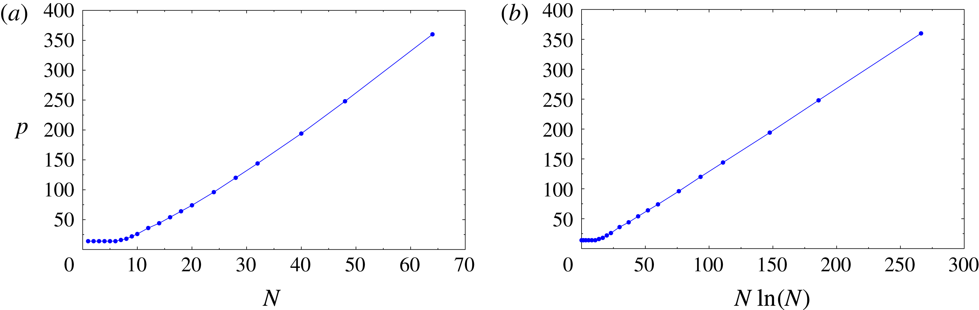
. The dependence of the thus determined minimum required arithmetic precision
 $p$
on the resolution
 $N$
is shown in figure 4. The change of trend observed in this figure for small
 $N$
is due to the fact that for such small resolutions the standard double precision (corresponding to
 $p=14$
) is sufficient. In figure 4(b), we see that for ‘large’
 $N$
, the required precision
 $p$
grows in proportion to
 $N\ln (N)$
, with the approximate relationship
 $p\approx 1.3843\,N\ln (N)-9.1422$
obtained with linear regression. Use of this relation to extrapolate the data shown in figure 4 indicates that to solve the problem with a resolution of
 $N=128$
, arithmetic precision with approximately
 $p=850$
significant digits would be required (the RAM memory needed to solve the Riccati equation with such values of
 $N$
and
 $p$
would exceed 128 GB). The data presented in figure 4 will guide our choice of the arithmetic precision in computations with different resolutions
 $N$
discussed in § 5.
Dependence of the minimum arithmetic precision
 $p$
required for an accurate solution of the Riccati equation (3.24) and determination of the feedback kernels
 $\boldsymbol{K}$
on (a) the resolution
 $N$
and (b) the quantity
 $N\ln (N)$
. For ‘large’
 $N$
, a clear scaling
 $p\sim N\ln (N)$
is evident in (b).
In the numerical integration of the closed-loop systems (3.25) and (3.26) the same arithmetic precision
 $p$
is used as in the solution of the Riccati equation (3.24) at the given resolution
 $N$
. The linear problem (3.25) is already an ODE system and is integrated using a multiprecision version of MATLAB’s adaptive time-stepping routine ode45 provided by Advanpix (Advanpix 2017). The relative and absolute tolerance are both set to
 $10^{-10}$
which in the course of extensive tests was found to ensure converged results.
The nonlinear closed-loop system (3.26) is discretized in space using the collocation approach devised by Sakajo & Okamoto (Reference Sakajo and Okamoto1996), but without regularization, on a mesh consisting of
 $2(N+1)$
equispaced grid points, which ensures that solution components with wavenumbers up to
 $N$
are resolved. The resulting ODE system is integrated in time using the multiprecision ode45 routine (Advanpix 2017). The relative and absolute tolerance are both set to
 $10^{-8}$
, which in the course of extensive tests was found to ensure converged results. We note that with sufficient arithmetic precision there is no need to use the spectral-filtering technique introduced by Krasny (Reference Krasny1986b
) to control the spurious growth of round-off errors. The operator
 ${\mathcal{F}}$
appearing in (3.26) is discretized using discrete Fourier-transform techniques, and, assuming that complex numbers are represented as pairs of real numbers, the resulting matrix
 $\unicode[STIX]{x1D641}$
has dimensions
 $4N\times 4(N+1)$
, where the difference in the two dimensions comes from the fact that the zero mode is not included in the spectral representation; cf. § 3.3. The matrix
 $\unicode[STIX]{x1D641}^{-1}$
is then defined as a pseudoinverse of
 $\unicode[STIX]{x1D641}$
with entries given analytically in terms of the inverse discrete sine and cosine transforms. A thorough assessment of the behaviour of the linear and nonlinear closed-loop systems (3.25) and (3.26) as functions of several different parameters is offered in the next section.
5 Results
In this section, we present a number of computational results illustrating the behaviour of the linear and nonlinear closed-loop systems (3.25) and (3.26), where we will analyse the influence of the different parameters characterizing the actuation; cf. § 2.2. This will allow us to assess to what degree the properties established theoretically for the linear problem in § 3.2 can be extended to the nonlinear setting. The use of point vortices, rather than point sinks/sources, as actuation results in essentially identical performance of the closed-loop system in the linear case and very similar performance in the nonlinear case. Therefore, for brevity, we will restrict the presentation of our results here to actuation with point sinks/sources. To focus attention, unless stated otherwise, we will consider actuation with varying numbers
 $N_{c}$
of sink/source pairs in the aligned arrangement (cf. figure 3
a) at a distance
 $b_{0}=1.0$
from the sheet in its undisturbed configuration, whereas the relative cost of control appearing in (3.20) will be
 $r=1.0$
. In all cases, the initial condition
 $z_{0}$
will be constructed by superposing a suitably scaled perturbation
 $\unicode[STIX]{x1D701}_{0}$
on the equilibrium configuration
 $\tilde{z}$
, i.e.
 $z_{0}=\tilde{z}+\unicode[STIX]{x1D700}\,\unicode[STIX]{x1D701}_{0}$
, where the perturbation will be taken as the sum of two unstable eigenfunctions
 $\unicode[STIX]{x1D709}_{1}$
and
 $\unicode[STIX]{x1D709}_{2}$
, cf. (2.15a
)–(2.15b
),
 $$\begin{eqnarray}\unicode[STIX]{x1D701}_{0}=\unicode[STIX]{x1D709}_{1}+\unicode[STIX]{x1D709}_{2},\end{eqnarray}$$
with wavenumber
 $n_{0}$
that, unless stated otherwise, will be
 $n_{0}=1$
; cf. figure 2. The ‘size’ of the initial perturbation determined by
 $\unicode[STIX]{x1D700}$
will play an important role in the nonlinear case, but is irrelevant in the linear setting. Due to the reasons detailed in § 4, the numerical resolution used in most of the computations discussed below is rather modest and is given by
 $N=31$
, corresponding to
 $N_{x}=64$
grid points in the ‘physical’ space and the system dimension of 128. At this resolution, the required arithmetic precision is
 $p=144$
; cf. figure 4. We recall that, in the absence of control, the Birkhoff–Rott system (2.2) exhibits a finite-time blow-up manifested by the appearance of a curvature singularity. In order to verify the analysis from § 3.1, we first investigate the borderline case with the smallest possible number
 $N_{c}=N+1$
of actuator pairs and then focus on the more relevant cases when
 $N_{c}\geqslant N+1$
.
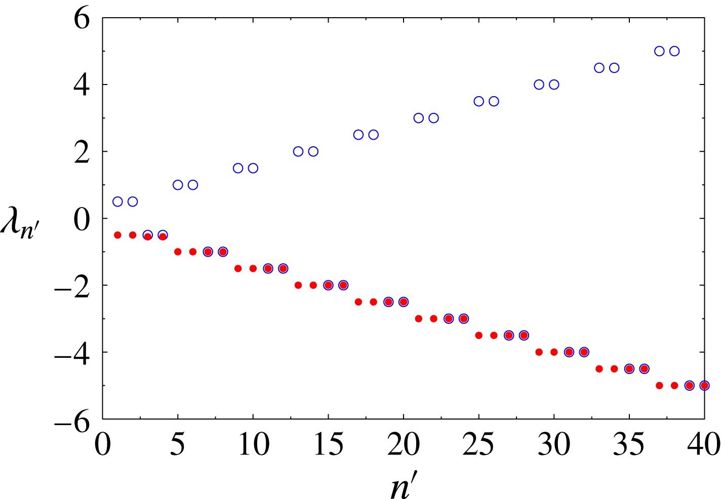
Eigenvalues of the linear open-loop system (2.11) (empty blue circles) and the closed-loop system (3.25) (filled red circles) for the resolution
 $N=31$
and actuation with
 $N_{c}=N+1=32$
pairs of sinks/sources. The index
 $n^{\prime }$
is defined such that
 $n=(n^{\prime }\hspace{0.6em}{\rm mod}\hspace{0.2em}4)$
, and, for clarity, only eigenvalues with small magnitude are shown.
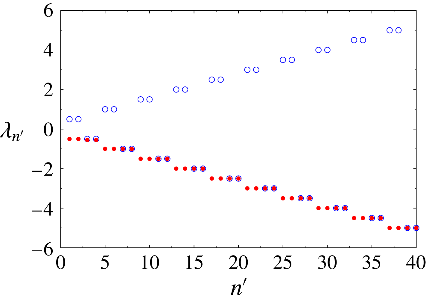
To begin, we show the eigenvalues of the linear open-loop and closed-loop systems (2.11) and (3.25) in figure 5. In the uncontrolled case, at every wavenumber
 $n$
, there are two positive and two negative eigenvalues,
 $\unicode[STIX]{x1D706}_{n}^{+}$
and
 $\unicode[STIX]{x1D706}_{n}^{-}$
; cf. § 2.1. In the controlled case, the originally unstable eigenvalues
 $\unicode[STIX]{x1D706}_{n}^{+}$
have their signs reversed with magnitude approximately retained. The matrix
 $(\unicode[STIX]{x1D63C}-\unicode[STIX]{x1D63D}^{Q}\boldsymbol{K})$
of the linear closed-loop system is not block-diagonal and normal, in contrast to the matrix
 $\unicode[STIX]{x1D63C}$
of the open-loop system; cf. § 2.1. However, the degree of its non-normality is fairly weak and decreases as the number
 $N_{c}$
of actuator pairs increases.
Dependence of (a) the perturbation energy
 $\Vert y(t)\Vert _{2}^{2}$
and (b) the actuation energy
 $\Vert \unicode[STIX]{x1D63D}^{Q}\boldsymbol{g}(t)\Vert _{2}^{2}$
on time
 $t$
for a system discretized with increasing resolution
 $N=15,31,63$
(the trends with increasing
 $N$
are indicated with arrows). The initial perturbation, cf. (5.1), is scaled such that
 $\Vert \unicode[STIX]{x1D700}\unicode[STIX]{x1D701}_{0}\Vert _{\infty }=0.02$
, whereas the actuation uses the smallest possible number of sink/source pairs,
 $N_{c}=N+1$
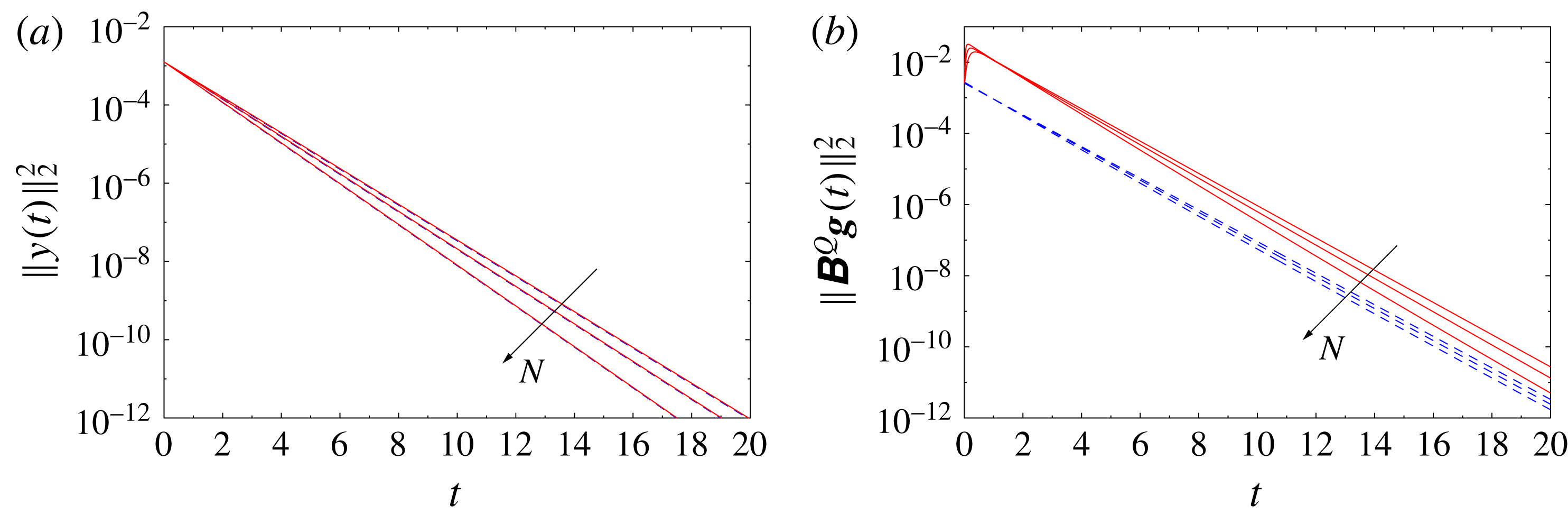
; cf. (3.15). The data for the linear and nonlinear problems are shown with dashed blue and solid red lines respectively.

Next, we analyse the ‘continuous limit’ of the problem when the resolution
 $N$
and the number
 $N_{c}$
of sink/source pairs both increase such that
 $N_{c}=N+1$
. We note that in the limit
 $N_{c}\rightarrow \infty$
, each of the actuator arrays may be regarded as approximating a continuous distribution of blowing and suction on hypothetical walls; cf § 2.2 and figure 1. The histories of the perturbation energy
 $\Vert y(t)\Vert _{2}^{2}$
and the corresponding actuation energy
 $\Vert \unicode[STIX]{x1D63D}^{Q}\boldsymbol{g}(t)\Vert _{2}^{2}$
, cf. (3.19)–(3.20), are shown for different values of
 $N$
and
 $N_{c}$
for the linear and nonlinear cases in figures 6(a) and 6(b) respectively. In figure 6(a), we see that there is very little difference in the behaviour between the linear and nonlinear cases, and in both cases the perturbation energy
 $\Vert y(t)\Vert _{2}^{2}$
vanishes exponentially, with the rate of decay increasing with
 $N$
(and therefore also with
 $N_{c}$
). On the other hand, in figure 6(b), we see that the required control effort in the nonlinear case is larger than that in the linear case. In addition, while in the linear case the actuation energy vanishes exponentially for all times
 $t>0$
, in the nonlinear case it first increases before eventually decaying exponentially with the rate increasing with
 $N_{c}=N+1$
. We remark that the data presented in figures 6(a) and 6(b) correspond to initial perturbations with magnitude
 $\Vert \unicode[STIX]{x1D700}\unicode[STIX]{x1D701}_{0}\Vert _{\infty }=0.02$
, which is close to the magnitude of the largest perturbations that can be stabilized in the nonlinear case using the smallest possible number of actuator pairs,
 $N_{c}=N+1$
; cf. (3.15).
Now, we move on to characterize the behaviour of the linear and nonlinear closed-loop systems (3.25) and (3.26) as the number
 $N_{c}$
of actuator pairs is varied while the resolution
 $N$
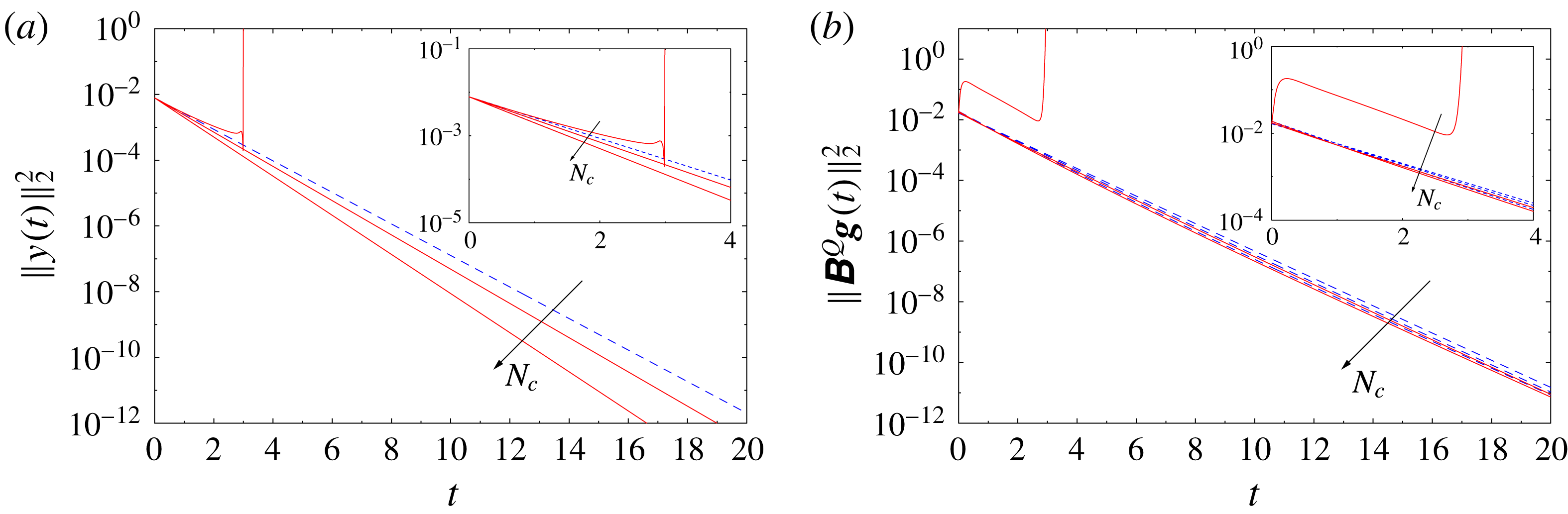
remains fixed. The histories of the perturbation energy
 $\Vert y(t)\Vert _{2}^{2}$
and the actuation energy
 $\Vert \unicode[STIX]{x1D63D}^{Q}\boldsymbol{g}(t)\Vert _{2}^{2}$
are shown in figures 7(a) and 7(b) respectively, with insets offering magnifications of the initial stages. The magnitude of the initial perturbation, cf. (5.1), is
 $\Vert \unicode[STIX]{x1D700}\unicode[STIX]{x1D701}_{0}\Vert _{\infty }=0.05$
in all cases. We see that in the linear problems, the decay of the perturbation energy is exponential in all cases, with the rate of decay increasing for larger
 $N_{c}$
, and the same is also true for the behaviour of the actuation energy. On the other hand, in the nonlinear regime, we observe that the perturbation cannot be stabilized when the smallest possible number
 $N_{c}=32$
of actuator pairs is used, and the solution blows up in finite time in that case. We note that with this number of actuators, it was possible to stabilize perturbations with a smaller magnitude; cf. figure 6. This demonstrates that the nonlinear problem may not be stabilized if the magnitude of the initial perturbation
 $\unicode[STIX]{x1D700}\unicode[STIX]{x1D701}_{0}$
exceeds a certain threshold, even if the corresponding linear problem is controllable. When larger numbers of actuators are used, the perturbation energy in the solutions of the nonlinear closed-loop problems behaves similarly to its behaviour in the solutions of the linear closed-loop problems. However, close inspection of figure 7(b) indicates that when a larger number of actuator pairs is used,
 $N_{c}\geqslant 2(N+1)$
, the actuation energy required to stabilize the nonlinear system is in fact slightly smaller than the actuation energy required to stabilize the corresponding linear system. As is evident from figure 6(b), the opposite occurs when
 $N_{c}=N+1$
.
Dependence of (a) the perturbation energy
 $\Vert y(t)\Vert _{2}^{2}$
and (b) the actuation energy
 $\Vert \unicode[STIX]{x1D63D}^{Q}\boldsymbol{g}(t)\Vert _{2}^{2}$
on time
 $t$
for a system discretized with the resolution
 $N=31$
and with different numbers of actuator pairs,
 $N_{c}=32,64,128$
(the trend with increasing
 $N_{c}$
is indicated with arrows). The initial perturbation, cf. (5.1), is scaled such that
 $\Vert \unicode[STIX]{x1D700}\unicode[STIX]{x1D701}_{0}\Vert _{\infty }=0.05$
. The insets represent magnifications of the initial stages. The data for the linear and nonlinear problems are shown with dashed blue and solid red lines respectively.
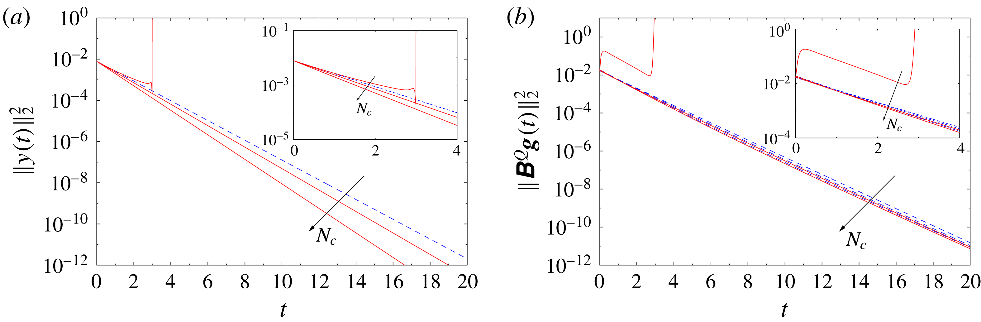
Evolution of the solutions to the linear and nonlinear closed-loop problems obtained with resolution
 $N=31$
,
 $N_{c}=64$
sink/source pairs and the initial data scaled such that
 $\Vert \unicode[STIX]{x1D700}\unicode[STIX]{x1D701}_{0}\Vert _{\infty }=0.2$
in (a) the physical space and (b) the Fourier space at a number of representative time instances (the trends with increasing
 $t$
are indicated with arrows). In (a), the data for the linear and nonlinear problems are shown with dashed blue and solid red lines respectively, whereas the thick black solid line represents the initial condition
 $z_{0}$
; in (b), the data for the linear and nonlinear problems are shown with blue squares and red circles respectively, whereas the black diamond represents the initial condition
 $z_{0}$
.
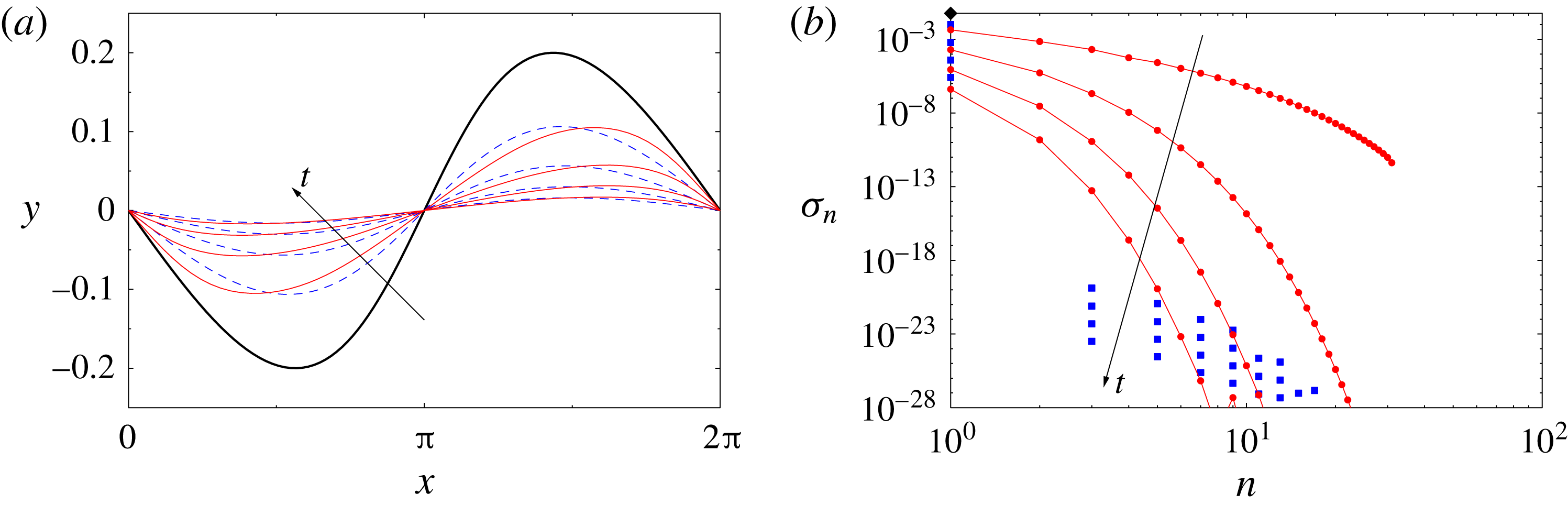
To focus attention, in the remainder of this section, we consider the case with the resolution
 $N=31$
,
 $N_{c}=64$
actuator pairs (which is twice as many as the minimum number required for controllability in the linear case for the given resolution
 $N$
; cf. (3.15)) and the initial perturbation scaled such that
 $\Vert \unicode[STIX]{x1D700}\unicode[STIX]{x1D701}_{0}\Vert _{\infty }=0.2$
. We now analyse the time evolution of the solution to the representative problem defined above in the ‘physical’ space in figure 8(a) and in the Fourier-space representation in terms of the quantity
 $\unicode[STIX]{x1D70E}_{n}=(1/4)(|\unicode[STIX]{x1D6FC}_{-n}|+|\unicode[STIX]{x1D6FD}_{n}|+|\unicode[STIX]{x1D6FD}_{-n}|+|\unicode[STIX]{x1D6FC}_{n}|)$
,
 $n=1,\ldots ,N$
, in figure 8(b). In figure 8(a), we note that, as the control starts to act, the initial perturbation is attenuated without much change of shape in both the linear and nonlinear settings. This behaviour is also reflected in the corresponding evolution in the Fourier space shown in figure 8(b), where we see that the control attenuates the spectrum of the solution uniformly across all wavenumbers, and in the linear problem there is little energy transfer from the mode with
 $n_{0}=1$
to modes with higher wavenumbers. This latter property is a consequence of the fact that the closed-loop linear system is only weakly non-normal. In the nonlinear case, the amplitude of the Fourier components with wavenumbers
 $n>1$
is larger than in the linear case, which is a consequence of the nonlinear energy transfer. Next, in figure 9, we present the corresponding histories of individual actuator intensities in the form of ‘cascade plots’. We see that in the linear problem, the intensities of actuators in both the upper and lower arrays, respectively
 $[g_{1},g_{3},\ldots ,g_{2N_{c}-1}]$
and
 $[g_{2},g_{4},\ldots ,g_{2N_{c}}]$
, at all times exhibit a smooth wave-like dependence on the actuator index (which is proportional to its
 $x$
coordinate). There is a certain phase shift between intensities of actuators in the two arrays. On the other hand, in the nonlinear problem, the actuator intensities at early times reveal a fairly irregular dependence on the actuator index, with neighbouring actuators often having intensities of opposite signs; cf. figure 9(c,d). However, the magnitudes of the actuator intensities in the nonlinear problem also exhibit a wave-like envelope similar to the behaviour observed in the linear problem in figure 9(a,b). At initial times, the actuator intensities in the nonlinear problem are significantly larger, by a few orders of magnitude, than the corresponding actuator intensities in the linear problem, although this difference vanishes as the magnitude
 $\Vert \unicode[STIX]{x1D700}\unicode[STIX]{x1D701}_{0}\Vert _{\infty }$
of the initial perturbation decreases (this result is not shown here). Interestingly, the corresponding energy
 $\Vert \unicode[STIX]{x1D63D}^{Q}\boldsymbol{g}(t)\Vert _{2}^{2}$
of the velocity field induced by the actuation at the vortex sheet in its undeformed configuration is actually smaller in the nonlinear problem than in the linear case; see figures 10(b) and 11(b) discussed below. The reason is that when neighbouring actuators have intensities of opposite signs, this effect is cancelled when the velocity they induce at the sheet location is computed as
 $\unicode[STIX]{x1D63D}^{Q}\boldsymbol{g}(t)$
.
Time histories of the intensities of individual actuators in the solution to (a,b) the linear and (c,d) the nonlinear closed-loop problem with resolution
 $N=31$
using
 $N_{c}=64$
actuator pairs and the initial perturbation scaled such that
 $\Vert \unicode[STIX]{x1D700}\unicode[STIX]{x1D701}_{0}\Vert _{\infty }=0.2$
. Panels (a,c) and (b,d) correspond to actuators in the upper and lower arrays (cf. figure 1), where the actuator index is defined as
 $k^{\prime }=(k+1)/2$
,
 $k=1,3,\ldots ,2N_{c}-1$
, and
 $k^{\prime }=k/2$
,
 $k=2,4,\ldots ,2N_{c}$
, respectively. For clarity, only short times
 $t\in [0,0.1]$
are shown.
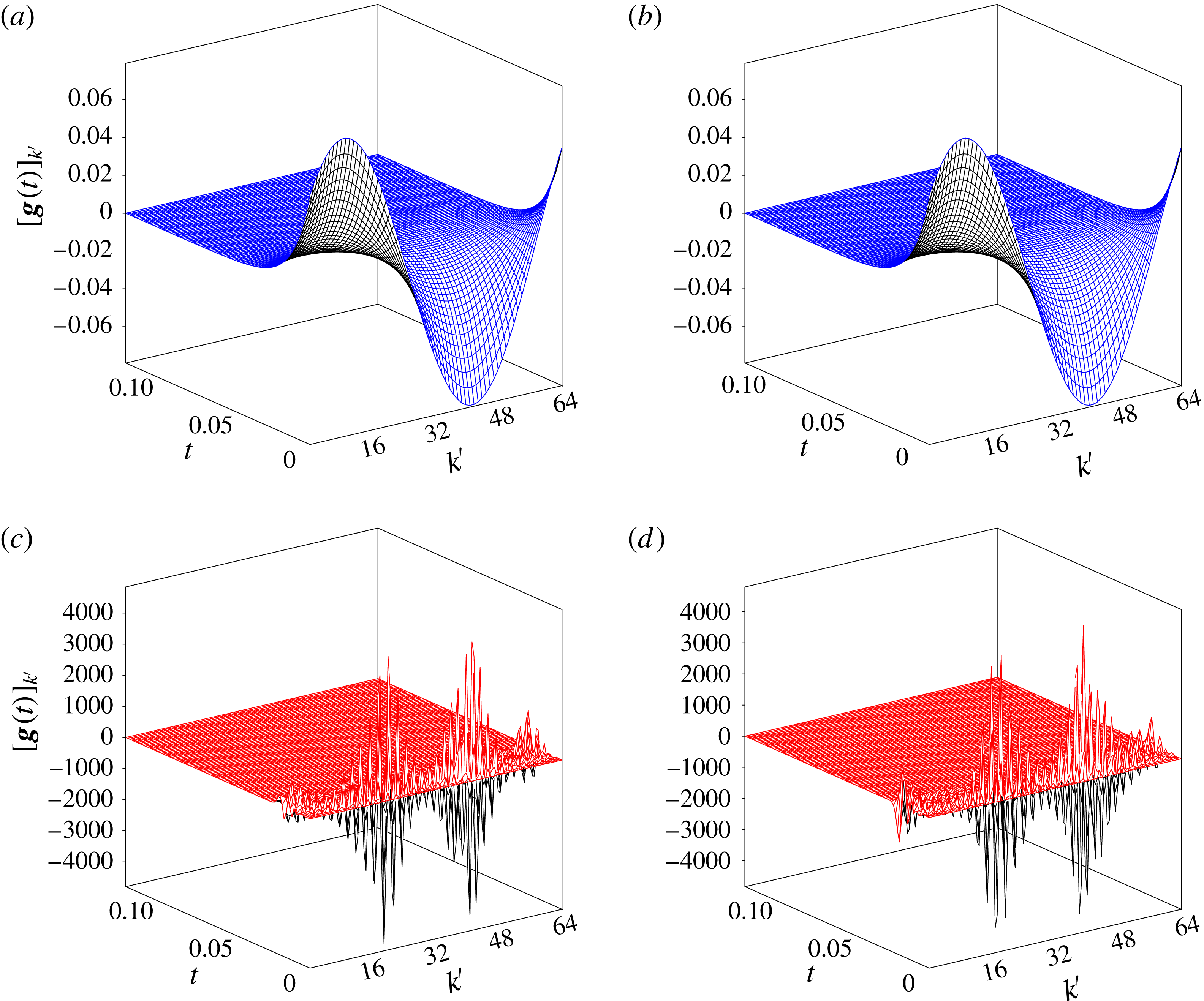
In the remaining parts of this section, we will study how the performance of the closed-loop control in the linear and nonlinear settings is influenced by a number of parameters characterizing the problem. First, we investigate the effect of the parameter
 $b_{0}$
describing the separation of the actuators from the vortex sheet in its unperturbed configuration; cf. § 2.2. In figure 10(a), we see that, as expected, increase in the separation
 $b_{0}$
results in a reduction of the exponential decay rate of the perturbation energy in the linear closed-loop system, and an essentially identical trend is also evident in the evolution governed by the nonlinear closed-loop system. In figure 10(b), we observe that increase in the separation
 $b_{0}$
also tends to increase the actuation energy
 $\Vert \unicode[STIX]{x1D63D}^{Q}\boldsymbol{g}(t)\Vert _{2}^{2}$
required to stabilize the system, with that energy again being smaller in the nonlinear case than in the linear case; cf. figure 7(b).
Dependence of (a) the perturbation energy
 $\Vert y(t)\Vert _{2}^{2}$
and (b) the actuation energy
 $\Vert \unicode[STIX]{x1D63D}^{Q}\boldsymbol{g}(t)\Vert _{2}^{2}$
on time
 $t$
for different separations of the sinks/sources from the sheet,
 $b_{0}=0.1,1,1.5$
(the trends with increasing
 $b_{0}$
are indicated with arrows). The remaining parameters are
 $N=31$
,
 $N_{c}=64$
and
 $\Vert \unicode[STIX]{x1D700}\unicode[STIX]{x1D701}_{0}\Vert _{\infty }=0.2$
. The data for the linear and nonlinear problems are shown with dashed blue and solid red lines respectively.
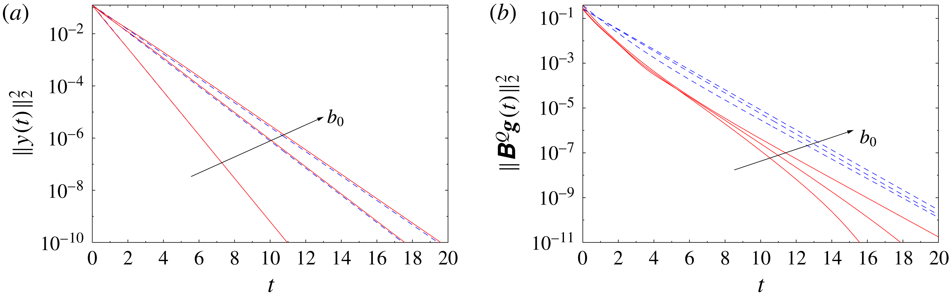
Dependence of (a) the perturbation energy
 $\Vert y(t)\Vert _{2}^{2}$
and (b) the actuation energy
 $\Vert \unicode[STIX]{x1D63D}^{Q}\boldsymbol{g}(t)\Vert _{2}^{2}$
on time
 $t$
for different costs of control,
 $r=10^{-2},1,10^{2}$
(the trends with increasing
 $r$
are indicated with arrows). The remaining parameters are
 $N=31$
,
 $N_{c}=64$
and
 $\Vert \unicode[STIX]{x1D700}\unicode[STIX]{x1D701}_{0}\Vert _{\infty }=0.2$
. The data for the linear and nonlinear problems are shown with dashed blue and solid red lines respectively.
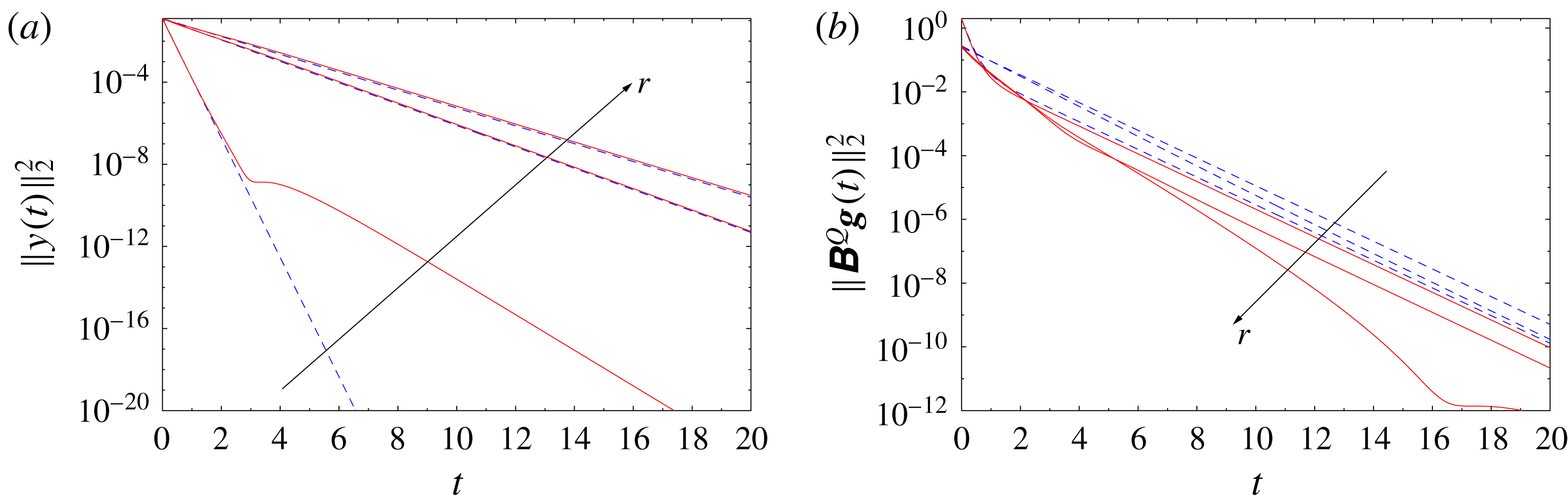
The influence of the relative cost of control,
 $r$
, cf. (3.20), on the performance of the control is documented in figure 11. In figure 11(a), we see that, as expected, increase in the cost
 $r$
results in a reduction of the exponential decay rate of the perturbation energy in the linear closed-loop system, and similar trends are also evident in the evolution governed by the nonlinear closed-loop system, except for the case with
 $r=10^{-2}$
when at later times the convergence slows down. This can be attributed to the fact that with a low cost of control, the actuation may act more ‘aggressively’, which may not be desirable in the nonlinear setting. In figure 11(b), we note that increase in the value of
 $r$
tends to reduce the actuation energy
 $\Vert \unicode[STIX]{x1D63D}^{Q}\boldsymbol{g}(t)\Vert _{2}^{2}$
required to stabilize the system, with that energy again being smaller in the nonlinear case than in the linear case; cf. figure 7(b). We also note that the variation of the actuation energy is not very significant, even though the considered values of
 $r$
span four orders of magnitude, which may suggest that in actual applications it may be advisable to consider ways of penalizing the control effort other than proposed in (3.20)–(3.22).
We close this section by analysing the performance of the linear and nonlinear closed-loop systems (3.25) and (3.26) with initial perturbations characterized by different wavenumbers
 $n_{0}$
. We continue to focus on the case with resolution
 $N=31$
and
 $N_{c}=64$
actuator pairs, but will now consider initial perturbations with wavenumbers
 $n_{0}=1,2,4$
, all scaled such that
 $\Vert \unicode[STIX]{x1D700}\unicode[STIX]{x1D701}_{0}\Vert _{\infty }=0.2$
. In figure 12(a), we see that the linear closed-loop evolution for the initial perturbations with different wavenumbers
 $n_{0}$
exhibits a purely exponential decay, with rates consistent with the dependence of the closed-loop eigenvalues on
 $n$
shown in figure 5. In the corresponding nonlinear problems, the decay of the perturbation energy is slightly slower, albeit still exponential, with the difference between the two cases increasing with
 $n_{0}$
. Analogous trends are also observed in figure 12(b) as regards the dependence of the actuation energy on time
 $t$
for initial perturbations with different wavenumbers
 $n_{0}$
. Finally, in figure 13, we analyse the performance of feedback stabilization in situations when the initial perturbation contains components with different wavenumbers, as happens in practice (cf. figure 2). We consider the case when
 $\unicode[STIX]{x1D701}_{0}$
is constructed as a superposition of Fourier components with wavenumbers
 $n_{0}=1,2,3,4$
with equal magnitude and scaled such that
 $\Vert \unicode[STIX]{x1D700}\unicode[STIX]{x1D701}_{0}\Vert _{\infty }=0.2$
, which is compared with the case when, as before, the initial perturbation has only one Fourier component with
 $n_{0}=1$
. In figure 13(a), we see that in both cases the perturbation energy vanishes exponentially with the same rate, which is determined by the slowest-decaying component (here, with
 $n_{0}=1$
present in both cases); cf. figure 5. In the case with the multicomponent initial perturbation, the decay of the perturbation energy in the nonlinear problem is a little slower than in the linear problem and is preceded by an increase of the actuation energy at the initial stages; cf. figure 13(b).
Dependence of (a) the perturbation energy
 $\Vert y(t)\Vert _{2}^{2}$
and (b) the actuation energy
 $\Vert \unicode[STIX]{x1D63D}^{Q}\boldsymbol{g}(t)\Vert _{2}^{2}$
on time
 $t$
for initial perturbations
 $\unicode[STIX]{x1D701}_{0}$
with different wavenumbers,
 $n_{0}=1,2,4$
(the trends with increasing
 $n_{0}$
are indicated with arrows). The remaining parameters are
 $N=31$
,
 $N_{c}=64$
and
 $\Vert \unicode[STIX]{x1D700}\unicode[STIX]{x1D701}_{0}\Vert _{\infty }=0.2$
. The data for the linear and nonlinear problems are shown with dashed blue and solid red lines respectively.
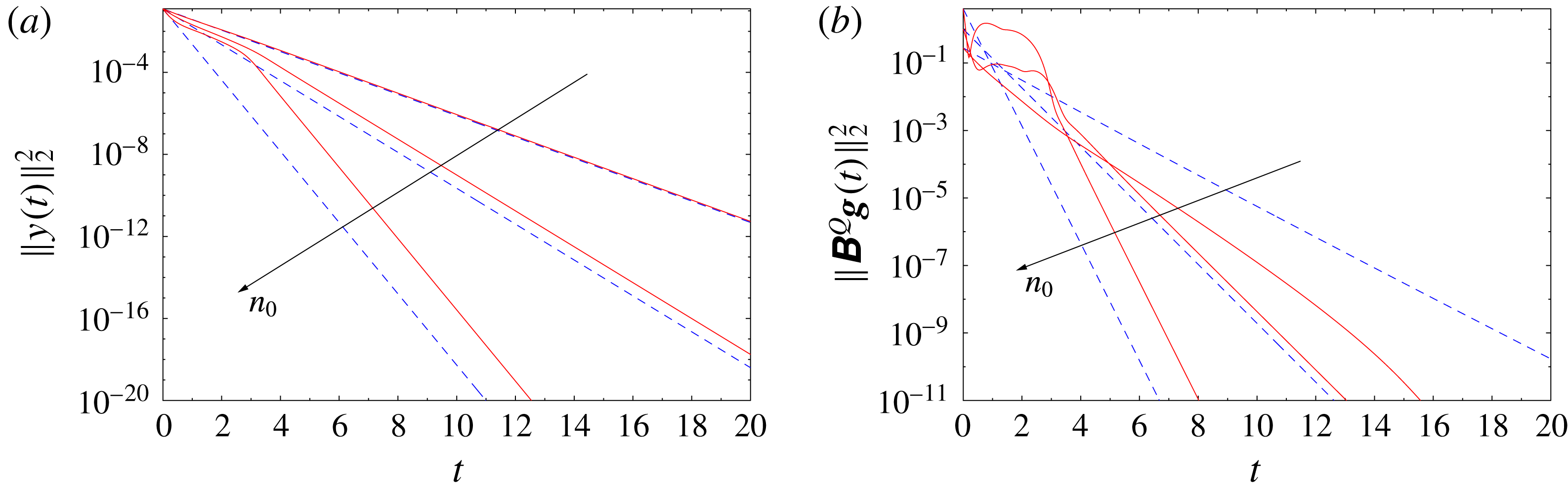
Dependence of (a) the perturbation energy
 $\Vert y(t)\Vert _{2}^{2}$
and (b) the actuation energy
 $\Vert \unicode[STIX]{x1D63D}^{Q}\boldsymbol{g}(t)\Vert _{2}^{2}$
on time
 $t$
for initial perturbations
 $\unicode[STIX]{x1D701}_{0}$
with a single wavenumber
 $n_{0}=1$
(thin lines) and constructed as a superposition of components with wavenumbers
 $n_{0}=1,2,3,4$
(thick lines). The remaining parameters are
 $N=31$
,
 $N_{c}=64$
and
 $\Vert \unicode[STIX]{x1D700}\unicode[STIX]{x1D701}_{0}\Vert _{\infty }=0.2$
. The data for the linear and nonlinear problems are shown with dashed blue and solid red lines respectively.
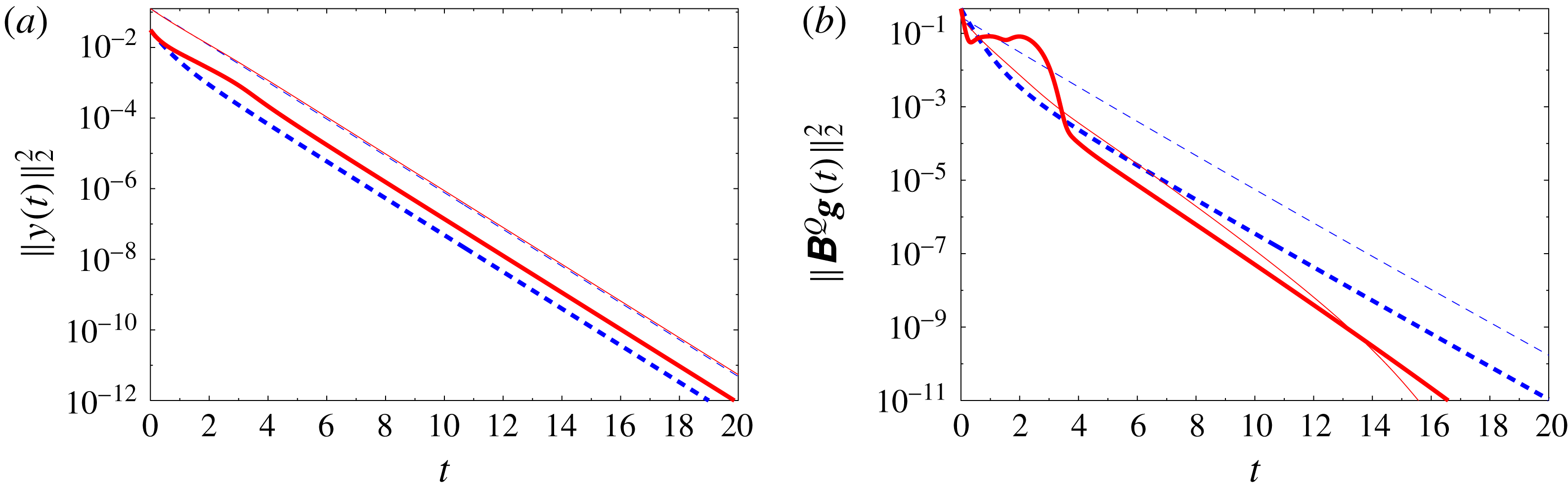
6 Discussion and conclusions
In this study, we have considered the problem of feedback stabilization of a flat inviscid vortex sheet described by the Birkhoff–Rott equation (2.2) as an idealized model for shear layers arising in many important applications. In addition to serving as a prototype of the Kelvin–Helmholtz instability, which is central to many vortex-dynamics phenomena, inviscid vortex sheets also give rise to many interesting mathematical problems related to the ill-posedness of the Birkhoff–Rott equation. While numerical solution of this equation typically requires a suitable regularization, we focused here on an admittedly harder problem when there is no regularization. There have already been many successful applications of the methods of linear control theory to flow problems (Kim & Bewley Reference Kim and Bewley2007; Bagheri et al. Reference Bagheri, Henningson, Hoepffner and Schmid2009), but only relatively few to inviscid vortex flows (Protas Reference Protas2008; Nelson et al. Reference Nelson, Protas and Sakajo2017), as they often give rise to a range of unique technical challenges, some of which are reiterated below.
As the first main finding of our study, we demonstrated using analytical computations that the Birkhoff–Rott equation linearized around the flat-sheet configuration is controllable when the number
 $N_{c}$
of actuator pairs is sufficiently large relative to the number of degrees of freedom present in the truncated Fourier representation of the equation, or, more specifically, when condition (3.15) is satisfied. This result holds when either point sinks/sources or point vortices are used as actuators and under the condition that their total mass flux or circulation is conserved in time independently for actuators located above and below the vortex sheet, cf. (2.19a
)–(2.19b
), which also guarantees global conservation of either mass or circulation. We focused here on actuation using point sinks/sources, because they represent typical experimental set-ups more accurately. However, feedback stabilization using point vortices as actuators gives essentially identical results. The controllability result holds for all generic actuator locations, except for the staggered arrangement shown in figure 3(b), where a larger number of actuator pairs is needed to ensure controllability. Therefore, in our study, we considered actuators in the aligned arrangement (cf. figure 3
a). Based on this controllability result, we designed a state-based LQR stabilization strategy where the key difficulty was the numerical solution of the Riccati equation (3.24) needed to determine the feedback kernel
 $\boldsymbol{K}$
, which is extremely ill-conditioned even for modest resolutions
 $N$
. This ill-conditioning is the result of the property that the unstable modes have growth rates proportional to the wavenumber
 $n$
, while the authority that the control actuation has over these modes vanishes as
 $\text{e}^{-n}$
, and was overcome by performing all computations with increased arithmetic precision depending on the resolution
 $N$
. It should be emphasized here that, unlike some other flow-control problems formulated in the spatially periodic setting (e.g. Bewley & Liu (Reference Bewley and Liu1998)), in the present case, the problem of determining the feedback kernels does not uncouple in the Fourier basis, and the Riccati equation (3.24) must be solved for all wavenumbers
 $n=1,\ldots ,N$
(the reason is that an actuator with the general form (3.4) simultaneously acts on solution components with all wavenumbers). An alternative approach would therefore be to consider actuation with two continuous distributions of blowing and suction whose intensities could be represented in terms of a finite number of Fourier modes. However, the formulation adopted in the present study is arguably more relevant and at the same time more interesting.
Computations performed for the linear closed-loop system revealed exponential decay of the perturbation energy and the corresponding actuation energy, with the decay rates changing in the expected ways as different parameters are varied, namely the number
 $N_{c}$
of actuator pairs, the distance
 $b_{0}$
between the actuators and the vortex sheet, the relative cost
 $r$
of the control and the wavenumber
 $n_{0}$
of the initial perturbation. In the nonlinear problems, initial perturbations can be stabilized provided that their magnitude is not too large, as otherwise a blow-up occurs in finite time (cf. figure 7
a), although its mechanism appears to be quite different from the singularity formation occurring in the original Birkhoff–Rott equation (2.2) (Moore Reference Moore1979). More precisely, while in both cases it takes place at times
 $O(1)$
for initial perturbations with the magnitude considered here, in the original Birkhoff–Rott equation (2.2), the singularity formation is signalled by the loss of analyticity by the solution, whereas in the problem with feedback stabilization (2.18), the
 $L^{2}$
norm of the solution blows up. However, it is important to note that as the number
 $N_{c}$
of actuator pairs increases, initial perturbations with larger magnitudes can be stabilized. More specifically, initial perturbations with the transverse amplitude equal to more than 3 % of the sheet length can be effectively stabilized. This insight is the second main finding of this study. The main objective of this investigation was to use a simple inviscid model of the vortex sheet dynamics given by the Birkhoff–Rott equation (2.2) to provide fundamental insights about the potential for stabilization of actual shear layers using feedback. Since with its ill-posedness the Birkhoff–Rott equation is a rather extreme example of instability, our findings indicate that, in principle, it may be possible to stabilize realistic shear layers, provided that the actuation has sufficiently many degrees of freedom.
When an initial perturbation can be stabilized in the nonlinear regime, the perturbation energy decays exponentially and the rate of decay is usually essentially the same as in the linear regime, except for cases when the cost of control
 $r$
is very small (cf. figure 11
a) and when the initial perturbations
 $\unicode[STIX]{x1D701}_{0}$
have wavenumbers
 $n_{0}>1$
(cf. figure 12
a). The corresponding actuation energy is larger than in the linear regime when the smallest possible number
 $N_{c}=N+1$
of actuator pairs is used (cf. figure 6
b), but becomes smaller than that when the number of actuator pairs is increased (cf. figure 7
b). It would be interesting to characterize the energetic efficiency of the proposed stabilization strategy in terms of the ratio of the kinetic energies of the flow perturbation and the actuation. However, due to limitations of our simple potential-flow model, the latter quantity is not well defined here, because the velocity field induced by a point singularity is not square-integrable over the flow domain; hence, such a quantitative comparison is not possible. We therefore used the quantities
 $\Vert y(t)\Vert _{2}^{2}$
and
 $\Vert \unicode[STIX]{x1D63D}^{Q}\boldsymbol{g}(t)\Vert _{2}^{2}$
as substitutes to represent the perturbation and actuation energy respectively. Likewise, the instantaneously large values of the control input
 $[g_{1}(t),\ldots ,g_{2N_{c}}(t)]$
observed in the nonlinear case for large initial perturbations, cf. figure 9(c,d), may also be regarded as an artefact related to modelling the actuation in terms of point singularities.
The perturbation energy was defined as a measure of the transverse deformation of the sheet. Our computations (not reported here) performed with an alternative definition of the perturbation energy based on the
 $L^{2}$
norm of the entire perturbation
 $\unicode[STIX]{x1D701}(t)$
, i.e. also involving its real (longitudinal) component, showed a qualitatively similar performance of the control, except that the actuation was less efficient as it also had to attenuate the longitudinal part of the perturbation (which is physically irrelevant as it amounts to merely reparameterizing the equilibrium configuration
 $\tilde{z}(\unicode[STIX]{x1D6FE})$
). Our analysis also demonstrated that the proposed feedback stabilization strategy exhibits the expected behaviour as different parameters (
 $b_{0}$
,
 $r$
and
 $n_{0}$
) are varied, although the dependence of the required actuation energy on its relative cost
 $r$
is rather weak, indicating that in actual applications different ways of penalizing the control effort may be preferable.
Let us finally discuss some future extensions of the present work towards more practical stabilization problems involving shear layers. The first step in this direction will be to investigate stabilization of vortex sheets under the influence of viscosity or surface tension (Hou et al.
Reference Hou, Lowengrub and Shelley1997) and of vortex layers with a finite thickness (Baker & Shelley Reference Baker and Shelley1990). It is known that both of these effects may significantly affect the stability of the original problem. For example, viscosity tends to suppress the growth of perturbations with higher wavenumbers, such that the Kelvin–Helmholtz instability resulting from such perturbations is only moderate. For some common regularizations, the high-wavenumber instability becomes weaker and may be entirely eliminated, which means that unstable modes may be restricted to a certain finite range of wavenumbers, say
 $[N_{1},N_{2}]$
. Then, if we set the number of actuator pairs as
 $N_{c}=2(N_{2}+1)$
, the viscous vortex sheet should be stabilizable with less actuation. As mathematical models of such effects, we can utilize the dissipative
 $\unicode[STIX]{x1D6FF}$
-regularization (Krasny Reference Krasny1986a
) or the dispersive
 $\unicode[STIX]{x1D6FC}$
-regularization (Holm et al.
Reference Holm, Nitsche and Putkaradze2006) of vortex sheets, which both reduce or suppress entirely the instability of higher-wavenumber modes (cf. figure 3 in Holm et al. (Reference Holm, Nitsche and Putkaradze2006)). In addition, since state-based feedback stabilization strategies are not very useful in practical situations, where typically only incomplete and often noisy measurements are available instead of full-state information, a more applicable approach would involve an output-based compensator combining a state estimator, such as some form of the Kalman filter, with LQR stabilization (Protas Reference Protas2004; Nelson et al.
Reference Nelson, Protas and Sakajo2017). This constitutes a natural extension of the state-feedback stabilization approach presented here, and, as a step in this direction, in appendix B, we address the companion question concerning observability of the linearized Birkhoff–Rott equation with pointwise velocity measurements. Finally, a feedback stabilization (or compensation) approach designed based on such an extended model can be applied to stabilize the Kelvin–Helmholtz instability of viscous shear layers modelled by the Navier–Stokes equation, where high-wavenumber perturbations are strongly suppressed by viscous effects, in the spirit of what was done by Protas (Reference Protas2004) in the context of the Bénard–von Kármán instability in the cylinder wake. Another related problem concerns stabilization of inviscid vortex sheets in other geometries such as the sphere (Sakajo Reference Sakajo2004b
), which may have interesting geophysical implications. We add that, in some applications, such as for example mixing enhancement, one may be interested in stabilizing the system selectively, by damping perturbations only with certain wavenumbers; this represents yet another possible extension of this study.
Acknowledgements
An anonymous referee is acknowledged for providing important insights about the role of constraints (2.19a )–(2.19b ). The authors are grateful to P. Holoborodko from Advanpix LLC for his assistance with arbitrary-precision computations required to determine the feedback operators. They also acknowledge the generous hospitality of the Fields Institute for Mathematical Sciences in Toronto where this work began during the Thematic Program on Multiscale Scientific Computing (January–April 2016). The first author acknowledges the JSPS Fellowship that he held at Kyoto University in 2017 and partial support through an NSERC (Canada) Discovery Grant. The second author was supported by JSPS Kakenhi(B) no. 26287023 and JSPS A3 Foresight Program.
Appendix A. Spectral representations of kernels
Derivation of the spectral representation (3.5) of the linearized Birkhoff–Rott equation with control relies on the Fourier-series expansion of the function
 $\cot (z)$
and its derivative. More specifically, the Fourier coefficients
 $\widehat{\unicode[STIX]{x1D6F7}}_{n}$
and
 $\widehat{\unicode[STIX]{x1D6F9}}_{n}$
of
 $\cot ((x-a-\text{i}b)/2)$
and
 $1/\sin ^{2}((x-a-\text{i}b)/2)$
are defined through the following identities:
 $$\begin{eqnarray}\displaystyle \cot \left({\displaystyle \frac{x-a-\text{i}b}{2}}\right) & = & \displaystyle \mathop{\sum }_{n=-\infty }^{\infty }\widehat{\unicode[STIX]{x1D6F7}}_{n}\,\text{e}^{\text{i}nx},\end{eqnarray}$$
 $$\begin{eqnarray}\displaystyle -{\displaystyle \frac{1}{2\sin ^{2}\left({\displaystyle \frac{x-a-\text{i}b}{2}}\right)}} & = & \displaystyle \mathop{\sum }_{n=-\infty }^{\infty }\widehat{\unicode[STIX]{x1D6F9}}_{n}\,\text{e}^{\text{i}nx}.\end{eqnarray}$$
We will assume that
 $x,a\in \mathbb{R}$
, and will consider two cases depending on whether
 $b\in \mathbb{R}\backslash \{0\}$
is positive or negative (we recall that
 $b$
represents the vertical location of an actuator; cf. § 2.2).
When
 $b>0$
, we have
 $$\begin{eqnarray}\displaystyle \cot \left({\displaystyle \frac{x-a-\text{i}b}{2}}\right) & = & \displaystyle \text{i}{\displaystyle \frac{\text{e}^{\text{i}(x-a-\text{i}b)/2}+\text{e}^{-\text{i}(x-a-\text{i}b)/2}}{\text{e}^{\text{i}(x-a-\text{i}b)/2}-\text{e}^{-\text{i}(x-a-\text{i}b)/2}}}=\text{i}{\displaystyle \frac{1+\text{e}^{-\text{i}(x-a-\text{i}b)}}{1-\text{e}^{-\text{i}(x-a-\text{i}b)}}}\nonumber\\ \displaystyle & = & \displaystyle \text{i}\left(1+{\displaystyle \frac{2\text{e}^{-\text{i}(x-a-\text{i}b)}}{1-\text{e}^{-\text{i}(x-a-\text{i}b)}}}\right)=\text{i}\left(1+2\text{e}^{-\text{i}(x-a-\text{i}b)}{\displaystyle \frac{1}{1-\text{e}^{-\text{i}(x-a-\text{i}b)}}}\right)\nonumber\\ \displaystyle & = & \displaystyle \text{i}\left(1+2\text{e}^{-\text{i}(x-a-\text{i}b)}\mathop{\sum }_{n=0}^{\infty }\text{e}^{-\text{i}n(x-a-\text{i}b)}\right)=\text{i}\left(1+2\mathop{\sum }_{n=1}^{\infty }\text{e}^{-\text{i}n(x-a-\text{i}b)}\right)\nonumber\\ \displaystyle & = & \displaystyle \text{i}\left(1+2\mathop{\sum }_{n=1}^{\infty }\text{e}^{-nb+\text{i}na}\text{e}^{-\text{i}nx}\right).\end{eqnarray}$$
The infinite summation in the third equality is absolutely convergent due to the fact that
 $|\text{e}^{-\text{i}(x-a-bi)}|=\text{e}^{-2b}<1$
. Hence, the series is differentiable term by term, which gives rise to the following spectral representation of
 $1/\sin ^{2}((x-a-\text{i}b)/2)$
:
 $$\begin{eqnarray}-{\displaystyle \frac{1}{2\sin ^{2}\left({\displaystyle \frac{x-a-\text{i}b}{2}}\right)}}=\text{i}\left(2\mathop{\sum }_{n=1}^{\infty }(-\text{i}n)\text{e}^{-nb+\text{i}na}\text{e}^{-\text{i}nx}\right)=2\mathop{\sum }_{n=1}^{\infty }n\text{e}^{-nb+\text{i}na}\text{e}^{-\text{i}nx}.\end{eqnarray}$$
On the other hand, when
 $b<0$
, owing to the fact that
 $|\text{e}^{\text{i}(x-a-\text{i}b)}|=|\text{e}^{b}|<1$
, we have
 $$\begin{eqnarray}\displaystyle \cot \left({\displaystyle \frac{x-a-\text{i}b}{2}}\right) & = & \displaystyle \text{i}{\displaystyle \frac{\text{e}^{\text{i}(x-a-\text{i}b)/2}+\text{e}^{-\text{i}(x-a-\text{i}b)/2}}{\text{e}^{\text{i}(x-a-\text{i}b)/2}-\text{e}^{-\text{i}(x-a-\text{i}b)/2}}}=\text{i}{\displaystyle \frac{\text{e}^{\text{i}(x-a-\text{i}b)}+1}{\text{e}^{\text{i}(x-a-\text{i}b)}-1}}\nonumber\\ \displaystyle & = & \displaystyle \text{i}\left(1-{\displaystyle \frac{2}{1-\text{e}^{\text{i}(x-a-\text{i}b)}}}\right)=\text{i}\left(1-2\mathop{\sum }_{n=0}^{\infty }\text{e}^{\text{i}n(x-a-\text{i}b)}\right)\nonumber\\ \displaystyle & = & \displaystyle \text{i}\left(1-2\mathop{\sum }_{n=0}^{\infty }\text{e}^{nb-\text{i}na}\text{e}^{\text{i}nx}\right)=\text{i}\left(-1-2\mathop{\sum }_{n=1}^{\infty }\text{e}^{nb-\text{i}na}\text{e}^{\text{i}nx}\right)\end{eqnarray}$$
and
 $$\begin{eqnarray}-{\displaystyle \frac{1}{2\sin ^{2}\left({\displaystyle \frac{x-a-\text{i}b}{2}}\right)}}=\text{i}\left(-2\mathop{\sum }_{n=1}^{\infty }(\text{i}n)\text{e}^{nb-\text{i}na}\text{e}^{\text{i}nx}\right)=2\mathop{\sum }_{n=1}^{\infty }n\text{e}^{nb-\text{i}na}\text{e}^{\text{i}nx}.\end{eqnarray}$$
In summary, the Fourier coefficients
 $\widehat{\unicode[STIX]{x1D6F7}}_{n}$
and
 $\widehat{\unicode[STIX]{x1D6F9}}_{n}$
, cf. (A 1)–(A 2), are for
 $b>0$
given by
 $$\begin{eqnarray}\displaystyle \widehat{\unicode[STIX]{x1D6F7}}_{n} & = & \displaystyle \left\{\begin{array}{@{}ll@{}}0, & n\geqslant 1,\\ \text{i}, & n=0,\\ 2\text{i}\text{e}^{-|n|b+\text{i}|n|a}, & n\leqslant -1,\end{array}\right.\end{eqnarray}$$
 $$\begin{eqnarray}\displaystyle \widehat{\unicode[STIX]{x1D6F9}}_{n} & = & \displaystyle \left\{\begin{array}{@{}ll@{}}0, & n\geqslant 0,\\ 2|n|\text{e}^{-|n|b+\text{i}|n|a}, & n\leqslant -1\\ \end{array}\right.\end{eqnarray}$$
and for
 $b<0$
by
 $$\begin{eqnarray}\displaystyle \widehat{\unicode[STIX]{x1D6F7}}_{n} & = & \displaystyle \left\{\begin{array}{@{}ll@{}}-2\text{i}\text{e}^{nb-\text{i}na}, & n\geqslant 1,\\ -\text{i}, & n=0,\\ 0, & n\geqslant 1,\end{array}\right.\end{eqnarray}$$
 $$\begin{eqnarray}\displaystyle \widehat{\unicode[STIX]{x1D6F9}}_{n} & = & \displaystyle \left\{\begin{array}{@{}ll@{}}2n\text{e}^{nb-\text{i}na}, & n\geqslant 1,\\ 0, & n\leqslant 0.\end{array}\right.\end{eqnarray}$$
Appendix B. Measurements and observability
We assume that the measurements have the form of the velocity recorded continuously in time at some point
 $z_{m}=x_{m}+\text{i}y_{m}$
located away from the vortex sheet, where without loss of generality we can assume that
 $y_{m}>0$
, i.e.
 $$\begin{eqnarray}U\left(z_{m}\right)={\displaystyle \frac{1}{4\unicode[STIX]{x03C0}\text{i}}}\int _{0}^{2\unicode[STIX]{x03C0}}\cot \left({\displaystyle \frac{z_{m}-z(\unicode[STIX]{x1D6FE},t)}{2}}\right)\,\text{d}\unicode[STIX]{x1D6FE}+\mathop{\sum }_{k=1}^{2N_{c}}{\displaystyle \frac{G_{k}}{4\unicode[STIX]{x03C0}\text{i}}}\cot \left({\displaystyle \frac{z_{m}-w_{k}}{2}}\right).\end{eqnarray}$$
This allows us to define the observation operator
 $\boldsymbol{h}$
as
 $$\begin{eqnarray}\boldsymbol{h}[z]=\left[\begin{array}{@{}c@{}}\text{Re}(U(z_{m}))\\ -\text{Im}(U(z_{m}))\end{array}\right],\end{eqnarray}$$
where the notation
 $\boldsymbol{h}[z]$
implies the dependence of the measurements on the state variable
 $z$
, which represents the instantaneous position of the sheet. We will be primarily interested in the state-to-measurements map represented by the first term on the right-hand side in (B 1).
In order to assess the observability of the Birkhoff–Rott equation (3.1) with measurements defined in (B 2) linearized around the flat-sheet configuration, we will follow a formalism analogous to the approach employed in §§ 3.1 and 3.2 to study controllability. Observability implies that complete information about the state of the system can in the limit
 $t\rightarrow \infty$
be deduced from the available measurements. First, we need to obtain the linearization of the observation operator (B 2), and using ansatz (2.3) we can write
 $$\begin{eqnarray}\boldsymbol{h}[z]=\boldsymbol{h}[\tilde{z}]+\unicode[STIX]{x1D700}\,\boldsymbol{h}^{\prime }[\tilde{z}]\unicode[STIX]{x1D701}+\mathit{O}(\unicode[STIX]{x1D700}^{2}),\end{eqnarray}$$
where
 $$\begin{eqnarray}\boldsymbol{h}^{\prime }[\tilde{z}]\unicode[STIX]{x1D701}=\left[\begin{array}{@{}c@{}}\text{Re}(U^{\prime }(z_{m})\unicode[STIX]{x1D701})\\ \text{Im}(U^{\prime }(z_{m})\unicode[STIX]{x1D701})\end{array}\right],\end{eqnarray}$$
with
 $$\begin{eqnarray}U^{\prime }(z_{m})\unicode[STIX]{x1D701}=-{\displaystyle \frac{1}{4\unicode[STIX]{x03C0}\text{i}}}\int _{0}^{2\unicode[STIX]{x03C0}}{\displaystyle \frac{\unicode[STIX]{x1D701}(\unicode[STIX]{x1D6FE})}{2\sin ^{2}\left({\displaystyle \frac{\unicode[STIX]{x1D6FE}-z_{k}}{2}}\right)}}\,\text{d}\unicode[STIX]{x1D6FE}.\end{eqnarray}$$
Assuming that the perturbation
 $\unicode[STIX]{x1D701}$
is given by the Fourier series (2.4) truncated at the wavenumber
 $N$
and converted to the real-valued representation as in (2.8), expression (B 4) can be approximated as
 $$\begin{eqnarray}\boldsymbol{h}^{\prime }[\tilde{z}]\unicode[STIX]{x1D701}\approx \unicode[STIX]{x1D643}\boldsymbol{X},\end{eqnarray}$$
where
 $\unicode[STIX]{x1D643}=[\unicode[STIX]{x1D643}_{1}~\unicode[STIX]{x1D643}_{2}\cdots \unicode[STIX]{x1D643}_{N}]$
is the observation matrix. System (3.12) with measurements (B 6) is then declared observable if the following condition holds (Stengel Reference Stengel1994):
 $$\begin{eqnarray}\text{Rank}\left[\begin{array}{@{}c@{}}\unicode[STIX]{x1D643}\\ \unicode[STIX]{x1D643}\unicode[STIX]{x1D63C}\\ \cdots \\ \unicode[STIX]{x1D643}\unicode[STIX]{x1D63C}^{N-1}\end{array}\right]=4N,\end{eqnarray}$$
which, given the block-diagonal structure of the matrix
 $\unicode[STIX]{x1D63C}$
, cf. § 2.1, is satisfied if and only if the rank condition given below simultaneously holds for all individual blocks, i.e.
 $$\begin{eqnarray}{\mathcal{R}}_{n}^{H}=\left[\begin{array}{@{}c@{}}\unicode[STIX]{x1D643}_{n}\\ \unicode[STIX]{x1D643}_{n}\unicode[STIX]{x1D63C}_{n}\\ \unicode[STIX]{x1D643}_{n}\unicode[STIX]{x1D63C}_{n}^{2}\\ \unicode[STIX]{x1D643}_{n}\unicode[STIX]{x1D63C}_{n}^{3}\end{array}\right]=4,\quad n\geqslant 1.\end{eqnarray}$$
Using expansions (2.4) and (A 2) in (B 5), we obtain
 $$\begin{eqnarray}\displaystyle U^{\prime }(z_{m})\unicode[STIX]{x1D701} & = & \displaystyle -{\displaystyle \frac{\text{i}}{2}}\mathop{\sum }_{n=-\infty }^{\infty }\widehat{\unicode[STIX]{x1D6F9}}_{-n}\,\widehat{\unicode[STIX]{x1D701}}_{n}\nonumber\\ \displaystyle & = & \displaystyle \mathop{\sum }_{n=1}^{\infty }n\text{e}^{-ny_{m}}[(\sin (nx_{m})-\text{i}\cos (nx_{m}))\unicode[STIX]{x1D6FC}_{n}+(\cos (nx_{m})+\text{i}\sin (nx_{m}))\unicode[STIX]{x1D6FD}_{n}],\qquad\end{eqnarray}$$
where in the second equality we also used identity (A 8). After truncating the series at
 $n=N$
and rearranging it into a form consistent with (B 4), we obtain the following expression for the
 $n$
th block
 $\unicode[STIX]{x1D643}_{n}$
of the observation matrix:
 $$\begin{eqnarray}\unicode[STIX]{x1D643}_{n}=n\text{e}^{-ny_{m}}\left[\begin{array}{@{}cccc@{}}0 & \cos (nx_{m}) & 0 & \sin (nx_{m})\\ 0 & -\sin (nx_{m}) & 0 & \cos (nx_{m})\end{array}\right].\end{eqnarray}$$
It can be verified using symbolic-algebra tools such as Maple that condition (B 8) does indeed hold for
 $n\geqslant 1$
, implying the observability of the matrix pairs
 $\{\unicode[STIX]{x1D63C}_{n},\unicode[STIX]{x1D643}_{n}\}$
,
 $n\geqslant 1$
, and hence the observability of system (3.12) with the measurements (B 6) in the limit
 $N\rightarrow \infty$
. We add that, as is evident from the form of expression (B 10), modes with increasing wavenumbers
 $n$
, while in principle observable, leave only an exponentially decreasing footprint on the measurements. Moreover, observability is lost when only one velocity component is observed; cf. (B 2).