1. Introduction
The compressible turbulent boundary layer (TBL), where vorticity, acoustic and entropy modes are highly coupled (Lele Reference Lele1994), is one of the most considered flow phenomena in fluid dynamics and engineering applications. As an intriguing topic in TBLs, the pressure fluctuation associated with turbulent structures has attracted extensive research efforts. Fundamentally, pressure fluctuations play a pivotal role in redistributing turbulent kinetic energy (Pope Reference Pope2000), thus facilitating the sustainability of turbulence (Tsinober Reference Tsinober2009). In practical engineering applications, the wall pressure fluctuation (WPF) of TBLs is closely related to some critical issues, such as noise generation and structural fatigue (Bull Reference Bull1996). Accordingly, shedding light on the physical mechanism of WPFs, especially those with extremely high amplitudes, significantly contributes to the low-noise design and control of advanced aircraft.
When focusing on the feature of pressure fluctuations in TBLs, compressibility is an effect definitely worth highlighting, which affects some key properties of WPFs, such as standard deviation, spectral characteristics and intermittency (Bernardini & Pirozzoli Reference Bernardini and Pirozzoli2011; Duan, Beekman & Martín Reference Duan, Beekman and Martín2011; Yu et al. Reference Yu, Liu, Fu, Tang and Yuan2022a , Reference Yu, Liu, Fu, Tang and Yuan2022b ). Compressibility involved in compressible flow is mainly represented by two types of effects (Zhang Reference Zhang2013; Hasan et al. Reference Hasan, Costa, Larsson, Pirozzoli and Pecnik2025): one corresponds to variation of the thermodynamic mean quantity of turbulence induced by heat transfer, which is called the extrinsic compressibility (EC) effects; the other causes significant variations of turbulent thermodynamic fluctuation quantities, especially associated with changes in fluid volume in response to pressure fluctuations, namely the intrinsic compressibility (IC) effects which are also termed as ‘true’ (Smits & Dussauge Reference Smits and Dussauge2006) or ‘genuine’ (Yu, Xu & Pirozzoli Reference Yu, Xu and Pirozzoli2019) compressibility effects. In other words, EC effects can exist at any Mach number and are also associated with the weak thermodynamic fluctuations within the limitation of Morkovin’s hypothesis (Hasan et al. Reference Hasan, Larsson, Pirozzoli and Pecnik2023), but IC effects work only at high enoughMach numbers (Hasan et al. Reference Hasan, Costa, Larsson, Pirozzoli and Pecnik2025). The most direct manifestation of IC effects is the occurrence of travelling wave-packet-like dilatation fluctuations exhibiting as the alternating positive and negative structure (APNS), which has been extensively reported recently (Duan, Beekman & Martín Reference Duan, Beekman and Martín2010; Yu et al. Reference Yu, Xu and Pirozzoli2019; Tang et al. Reference Tang, Zhao, Wan and Liu2020; Huang, Duan & Choudhari Reference Huang, Duan and Choudhari2022; Yu et al. Reference Yu, Zhou, Dong, Yuan and Xu2024; Baranwal, Donzis & Bowersox Reference Baranwal, Donzis and Bowersox2025; Toki et al. Reference Toki, Sousa, Chen, Camillo, Wagner and Scalo2025). Moreover, it has been shown that APNS efficiently strengthens the standard deviation and high-frequency part of spectra of WPFs (Zhang et al. Reference Zhang, Duan and Choudhari2017, Reference Zhang, Wan, Liu, Sun and Lu2022; Duan et al. Reference Duan2019; Huang et al. Reference Huang, Duan, Casper, Wagnild and Bitter2024), having potentially significant impact on extreme events of WPFs to be revealed.
1.1. Extreme events in wall-bounded turbulence
Originating in its highly intermittent nature (Jiménez Reference Jiménez2012), turbulent wall-bounded flow is known to undergo sporadic bursts characterised by rare and extreme fluctuations, which have high amplitudes of even several times the standard deviations. Exploring the statistical properties and generation mechanisms of the extreme events is of critical significance for risk evaluation, optimised design and predictive control (Sapsis Reference Sapsis2021). In recent decades, extreme events in wall-bounded turbulence have attracted considerable research interest in the community. Hack & Schmidt (Reference Hack and Schmidt2021) identified the coherent structures associated with extreme events in the dissipation of turbulent kinetic energy by conditional space–time proper orthogonal decomposition (Schmidt & Schmid Reference Schmidt and Schmid2019). They found that a varicose instability, inducing localised extrema in dissipation and production and driving the formation of a hairpin vortex, is the underlying mechanism. Focusing on the extreme events of wall quantities, many researchers are interested in wall shear stress. By concurrent measurement of the wall shear stress and corresponding three-dimensional velocity field, Sheng, Malkief & Katz (Reference Sheng, Malkief and Katz2009) identified the predominantly streamwise counter-rotating vortex corresponding to high wall shear stress. Hutchins et al. (Reference Hutchins, Monty, Ganapathisubramani, Ng and Marusic2011) and Gomit, de Kat & Ganapathisubramani (Reference Gomit, de Kat and Ganapathisubramani2018) highlighted the role of the interaction between outer-layer large structures and near-wall small vortices in generating events of high wall shear stress. Pan & Kwon (Reference Pan and Kwon2018) performed conditional sampling on numerical data and reported that extreme skin-friction events are associated with a finger-shaped large-scale sweeping motion extending to the outer layer. As for extremely low wall shear stress, often referring to the backflow, some similar progress concerning associated structures has been achieved (Lenaers et al. Reference Lenaers, Li, Brethouwer, Schlatter and Örlü2012; Cardesa et al. Reference Cardesa, Monty, Soria and Chong2019; Guerrero et al. Reference Guerrero, Lambert and Chin2020, Reference Guerrero, Lambert and Chin2022; Chen, Chung & Wan Reference Chen, Chung and Wan2023; Fei et al. Reference Fei, Wang, Lai, Wang and Xu2024).
More recently, additional attention has been paid to the extreme events of wall heat flux in compressible TBLs. Tong et al. (Reference Tong, Dong, Lai, Yuan and Li2022) revealed the coherent structures associated with extreme wall heat flux in a TBL at a free-stream Mach number of
 $M=2.25$
. They showed that a characteristic two-layer structure of temperature fluctuations accompanied by a strong sweep motion is the cause of extreme events. Further, we proposed conditional integral identities on wall shear stress and wall heat flux to quantify the momentum and energy transport in extreme events (Zhang et al. Reference Zhang, Wan, Dong, Liu, Sun and Lu2023), and found that the dominant mechanism of energy transport is shifted from viscous dissipation to pressure-dilatation work when
 $M$
changes from
 $M=2$
to
 $8$
, as at high
 $M=8$
near-wall APNSs are prevalent. Additionally, we apply this conditional integral identity to analyse extreme wall heat flux in the hypersonic boundary layer over a lifting body (Zhang et al. Reference Zhang, Liu, Wan, Sun, Lu, Chen and Dong2024a
). However, as for the extreme WPF events, the understanding of their characteristics remains particularly limited. Ghaemi & Scarano (Reference Ghaemi and Scarano2013) performed tomographic particle image velocimetry on a TBL of free-stream velocity
 $u_\infty =9\,\rm m\,s^{-1}$
and obtained the unsteady pressure field by integration of the Poisson pressure equation. They found that positive peaks of WPFs are associated with an upstream sweep of high-speed flow opposing a downstream ejection event, while the negative peaks are related to both the spanwise and quasi-streamwise vortices. Yin et al. (Reference Yin, Wu, Wang, Ren, Qu, Zhang and Liu2023) studied the conditional property of WPFs in a TBL at
 $M=2$
by splitting them into positive and negative families and compared turbulent scales, convection velocities and spatial relationships for each family. Limei et al. (Reference Limei, Yuan, Dong, Li and Tong2024) reported the effects of interactions of shock waves and TBLs on WPFs with extremely high amplitudes. However, in general, there are several fundamental questions that remain to be addressed as follows. What turbulent structures induce extreme WPF events at high Mach numbers? What physical mechanisms underlying these structures primarily generate extreme WPF events? Additionally, given the modulation of compressibility effects on pressure fluctuation properties, what is the systematic impact of compressibility effects on the above two concerns?
1.2. Generation of turbulent pressure fluctuations
The achieved research progress has shown that extreme events are closely related to the elementary coherent structures manifested in near-wall self-sustained regeneration cycles (Schoppa & Hussain Reference Schoppa and Hussain2002; Jiménez Reference Jiménez2013). However, turbulence exhibits non-local effects, which are crucial for its sustenance and directly corresponding to the non-Lagrangian nature of pressure fluctuations (Tsinober Reference Tsinober2009). The generation of extreme WPFs cannot be interpreted simply by local coherent structures. Pioneeringly, Chou (Reference Chou1945) derived the governing equation of pressure fluctuations in Poisson form from Navier–Stokes equations, and Kraichnan (Reference Kraichnan1956) pointed out two primary physical mechanisms generating pressure fluctuations in incompressible flows: the linear turbulence–mean flow interaction and the nonlinear turbulence–turbulence interaction. These two generation mechanisms lead to the pressure components of rapid pressure
 $p_r$
and slow pressure
 $p_s$
, respectively, which are termed according to their response rate to the change of the mean flow (Pope Reference Pope2000). By quantitatively characterising the contributions of rapid and slow pressure, Chase (Reference Chase1980, Reference Chase1987) and Howe (Reference Howe1998) developed the classic Chase–Howe model for predicting the frequency–wavenumber spectrum of WPFs. Focusing on the compressible turbulence, Sarkar (Reference Sarkar1992) introduced an additional pressure component, compressible pressure
 $p_c$
, to account for the contribution of compressibility effects. Foysi, Sarkar & Friedrich (Reference Foysi, Sarkar and Friedrich2004) performed Poisson-equation-based pressure decomposition in compressible channel flows, enabling the analysis to isolate the contributions from different mechanisms to pressure–strain correlations. Tang et al. (Reference Tang, Zhao, Wan and Liu2020) and Yu, Xu & Pirozzoli (Reference Yu, Xu and Pirozzoli2020) explored compressibility effects on properties of pressure fluctuations in channel flow utilising the pressure decomposition and stressed the dominant role of compressible pressure in the near-wall region at high Mach numbers. Recently, we extended and applied the pressure decomposition into compressible TBLs and illustrated wall-cooling effects on pressure fluctuations from the perspective of generation mechanisms (Zhang et al. Reference Zhang, Wan, Liu, Sun and Lu2022). Based on the reasonable separation of acoustic and vorticity modes by the pressure decomposition, we further reported the intrinsic scaling relations that the intensity of compressible pressure are monotonically enhanced with Mach number (Zhang et al. Reference Zhang, Liu, Wan, Sun, Lu, Chen and Dong2024b
), while the intensity of hydrodynamic pressure (original pressure fluctuation excluding compressible pressure) is independent of Mach number, and aligns with the incompressible distribution. In general, the Poisson-equation-based pressure decomposition has played an important role in studying the characteristics of pressure fluctuations, such as analysis of pressure source (Chang, Piomelli & Blake Reference Chang, Piomelli and Blake1999; Anantharamu & Mahesh Reference Anantharamu and Mahesh2020), wall echo effects (Gerolymos et al. Reference Gerolymos, Sénéchal and Vallet2007, Reference Gerolymos, Sénéchal and Vallet2013) and modelling of WPF spectra (Hu, Reiche & Ewert Reference Hu, Reiche and Ewert2017; Grasso et al. Reference Grasso, Jaiswal, Wu, Moreau and Roger2019; Yang & Yang Reference Yang and Yang2022).
1.3. Methodology and scope of this study
This work aims to elucidate the mechanisms of extreme events of WPFs in TBLs under different levels of compressibility effects. Direct numerical simulation (DNS) datasets of TBLs with two varying parameters, i.e. the free-stream Mach number and wall temperature, are analysed systematically. These two parameters are designed to progressively manifest the EC and IC effects, ranging from weak to strong. In particular, the statistical characteristics (e.g. intermittency) of WPFs from the perspective of the wavelet and spectrum are explored. Then, the turbulent coherent structures that can induce extreme events of WPFs are identified by conditionally volumetric average and analysed from a physical perspective. Furthermore, by leveraging the method of Poisson-equation-based pressure decomposition, elementary contributions of each physical generation mechanism to extreme pressure are quantitatively evaluated, thereby offering more profound physical insights.
The rest of the paper is structured as follows. Section 2 introduces the numerical methods of DNS and simulation set-ups; § 3 describes the measure of compressibility for various control parameters; § 4 demonstrates the feature of extreme WPFs according to statistics and wavelet analysis; § 5 proposes and applies the framework of conditional analysis to explore the mechanisms of generation of extreme events. Finally, § 6 summarises the main findings of this work.
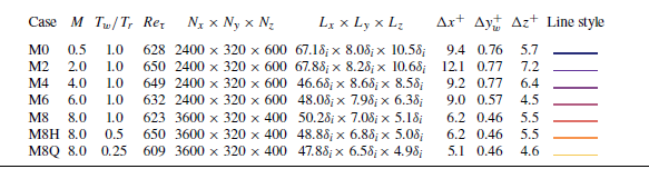
Simulation parameters of the compressible TBLs. Here
 $M$
is the free-stream Mach number;
 $T_w/T_r$
is the ratio of isothermal wall temperature to recovery temperature;
 $Re_\tau =\rho _w u_\tau \delta / \mu _{w}$
is the friction Reynolds number;
 $N$
and
 $L$
are the number of grid points and the length of the physical computational domain, respectively;
 $\Delta x^+$
and
 $\Delta z^+$
represent the streamwise and spanwise grid spacings in the wall unit; and
 $\Delta y^+_w$
denotes the wall-normal grid spacing at the wall.

2. Simulation of compressible turbulent boundary layers
Following our previous simulation work (Zhang et al. Reference Zhang, Wan, Liu, Sun and Lu2022, Reference Zhang, Liu, Wan, Sun, Lu, Chen and Dong2024b
), DNS of seven compressible flat-plate TBLs are performed by solving the fully compressible Navier–Stokes equations for the viscous and ideal gas. The efficient open-source code STREAmS (Bernardini et al. Reference Bernardini, Modesti, Salvadore and Pirozzoli2021), which can be accelerated markedly by graphics processing units, is used to conduct the simulations. The viscosity coefficient
 $\mu (T)$
of the ideal gas as a function of temperature is determined according to Sutherland’s law. To meet the resolution requirements of wall-bounded turbulence simulation, the equations are solved in a stretched Cartesian coordinate system and discretised by high-order finite-difference schemes. Specifically, hyperbolic sine stretching is applied in the wall-normal direction, and uniform grid spacing is set in the streamwise and spanwise directions of the physical computational domain. The convective term is spatially discretised using a hybrid energy-preserving/shock-capturing scheme in a locally conservative form. In smooth (shock-free) regions of the flow, the convective flux is approximated by the eighth-order energy-preserving scheme (Pirozzoli Reference Pirozzoli2010). While in discontinuous regions, the Lax–Friedrichs flux vector splitting ensures robust shock-capturing capabilities, and the seventh-order weighted essentially non-oscillatory scheme (Jiang & Shu Reference Jiang and Shu1996) is used to reconstruct the characteristic fluxes at interfaces. The viscous terms expanded to Laplacian form are approximated by the sixth-order central finite-difference formula. The three-stage, third-order Runge–Kutta scheme (Spalart, Moser & Rogers Reference Spalart, Moser and Rogers1991) is utilised to perform time integration. To establish a fully developed turbulent state, the inflow condition is set by the recycling–rescaling scheme (Pirozzoli, Bernardini & Grasso Reference Pirozzoli, Bernardini and Grasso2010), which brings less numerical pseudo-noise into TBLs than a synthetic inflow, such as the conventional digital filtering method (Ceci et al. Reference Ceci, Palumbo, Larsson and Pirozzoli2022). Non-reflecting boundary conditions (Poinsot & Lele Reference Poinsot and Lele1992) are imposed at the upper and outflow boundaries, according to the characteristic decomposition in the direction normal to the boundary. The boundary condition of the no-slip isothermal wall also applies a similar characteristic wave treatment. The periodic boundary condition is used in the spanwise direction. For further eliminating non-physical wave reflections, a buffer zone (Adams Reference Adams1998) is added around the top and end of the physical computation domain. For more details of the numerical methods, the reader is referred to the original paper introducing this STREAmS solver (Bernardini et al. Reference Bernardini, Modesti, Salvadore and Pirozzoli2021, Reference Bernardini, Modesti, Salvadore, Sathyanarayana, Della Posta and Pirozzoli2023b
).
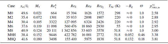
Statistics of the compressible TBLs. Here
 $x_a$
denotes the streamwise location for analysis. The friction Mach number and semi-local friction Reynolds number are
 $M_\tau =u_\tau /\sqrt {\gamma RT_w}$
and
 $Re_\tau ^\star =({\rho }_\infty \tau _w)^{1/2} \delta / {\mu }_{\infty }$
. The Reynolds number based on boundary-layer thickness is defined as
 $Re_{\delta }=\rho _{\infty } u_{\infty } \delta / \mu _{\infty }$
, and the Reynolds numbers based on momentum thickness as
 $Re_{\theta }=\rho _{\infty } u_{\infty } \theta / \mu _{\infty }$
and
 $Re_{\delta _{2}}=\rho _{\infty } u_{\infty } \theta / {\mu }_{w}$
, respectively. Temperature
 $T_\infty$
is the free-stream temperature,
 $B_{q}=-(\mathrm{d} \bar {T} / \mathrm{d} y^+)_w / Pr T_w$
indicates the non-dimensional wall heat flux,
 $\varTheta = (T_w-T_\infty )/(T_r - T_\infty )$
denotes the diabatic parameter and
 $p^{\prime +}_{rms,w}$
is the root mean square of wall pressure fluctuation in the wall unit.

The simulation parameters of seven compressible TBLs are shown in table 1. To examine both the EC and IC effects, five quasi-adiabatic cases with an
 $M$
range of
 $0.5\leqslant M \leqslant 8$
and two wall-cooling cases at
 $M=8$
are considered. For the quasi-adiabatic cases, the wall temperature
 $T_w$
is set equal to the recovery temperature
 $T_{r}=T_{\infty } (1+r(\gamma -1) M^{2} / 2 )$
based on a turbulent recovery factor of
 $r=0.89$
, and for the wall-cooling cases M8H and M8Q, the ratios
 $T_w/T_r$
are set to one half and one quarter, respectively. Similar friction Reynolds numbers of
 $Re_\tau \approx 630$
at the location for analysis are ensured for each case. The total grid size for every case is about 460 million. According to the grid spacing, higher grid resolutions are achieved in hypersonic TBLs for capturing finer turbulent structures at higher free-stream Reynolds numbers. Table 2 shows some basic statistics at the streamwise location for analysis. Increasing both the Mach number
 $M$
and the wall-cooling effect increase the friction Mach number
 $M_\tau$
. All the Reynolds numbers listed here increase with
 $M$
and decrease with enhanced wall-cooling effect. After reaching the supersonic regime, the non-dimensional WPF intensity
 $p^{\prime +}_{rms,w}$
increases slowly from 2.88 to 3.0. Notably, on further imposing wall cooling,
 $p^{\prime +}_{rms,w}$
is enhanced significantly in M8H and M8Q (Zhang, Duan & Choudhari Reference Zhang, Duan and Choudhari2017). It is worth mentioning that the typical first- and second-order turbulent statistics have been validated solidly by matching reference data in our previous work (Zhang et al. Reference Zhang, Wan, Liu, Sun and Lu2022, Reference Zhang, Liu, Wan, Sun, Lu, Chen and Dong2024b
), confirming the reliability of the current data.
In the following, the velocity variables are decomposed using the density-weighted (Favre) representation
 $f=\tilde {f}+f^{\prime \prime }$
, where
 $\tilde {f}=\overline {\rho f}/\bar {\rho }$
, and thermodynamics variables are decomposed using the standard Reynolds decomposition
 $f=\bar {f}+f^\prime$
. A superscript ‘+’ and subscript ‘
 $w$
’ denote the variable normalised by the wall unit and the variables at the wall, respectively.
Wall-normal distributions of (a) mean density
 $\bar {\rho }/\rho _\infty$
, (b) mean temperature
 $\bar {T}/{T}_\infty$
, (c) density fluctuations
 $\rho _{rms}^\prime /\bar {\rho }$
and (d) temperature fluctuations
 $T_{rms}^\prime /\bar {T}$
. The circles denote an
 $M=7.87$
TBL with
 $Re_{\tau }=480$
and
 $T_w/T_r=0.48$
from Zhang, Duan & Choudhari (Reference Zhang, Duan and Choudhari2018). For the line legend, see table 1.

3. Measure of compressibility
In this section, compressibility effects, encompassing both EC and IC effects, are comprehensively assessed through different characteristic statistics. Firstly, the wall-normal distributions of mean and root-mean-square of density and temperature are shown in figure 1. Aerodynamic heating by viscosity dominating near the wall makes the mean density and temperature vary from the reference value, exhibiting variable-property effects of EC. The influence of these effects on the mean and fluctuation velocity profiles can be accounted for by various velocity transforms (Van Driest Reference Van Driest1951; Volpiani et al. Reference Volpiani, Iyer, Pirozzoli and Larsson2020; Griffin, Fu & Moin Reference Griffin, Fu and Moin2021; Hasan et al. Reference Hasan, Larsson, Pirozzoli and Pecnik2023) and Morkovin scaling (Morkovin Reference Morkovin1962). When implementing cooling at the wall, the mean profiles of M8H and M8Q become non-monotonic. For root-mean-square fluctuations of density and temperature, our data of M8H are well consistent with those of Zhang et al. (Reference Zhang, Duan and Choudhari2018) indicated by circles with
 $M=7.78$
and
 $T_w/T_r=0.48$
. Increasing
 $M$
at the quasi-adiabatic condition monotonically enhances the fluctuations, while wall cooling suppresses the fluctuations except the near-wall region for M8H and M8Q. Bradshaw (Reference Bradshaw1977) suggested that Morkovin’s hypothesis may work when the root-mean-square of density fluctuations scaled by the mean density is below
 $10\,\%$
, and the upper limit of the applicable range for Mach number is 5. However, this evaluation is not accurate in that Morkovin’s hypothesis is still valid for cases where the Mach number is much higher than 5 with stronger density fluctuations (Lagha et al. Reference Lagha, Kim, Eldredge and Zhong2011; Duan et al. Reference Duan, Beekman and Martín2011). The key point of judgment should be the effects of IC (Hasan et al. Reference Hasan, Larsson, Pirozzoli and Pecnik2023). Hence, according to Coleman, Kim & Moser (Reference Coleman, Kim and Moser1995), the root-mean-square of pressure and total temperature fluctuations, when scaled by their respective means, serve as more effective evaluators for assessing the hypothesis.
Wall-normal distributions of
 $(a)$
pressure fluctuations
 $p_{rms}^{\prime }/\bar {p}$
,
 $(b)$
total temperature fluctuations
 $T_{0,rms}^{\prime }/\bar {T}$
,
 $(c)$
turbulent Mach numbers
 $M_t$
and
 $(d)$
dilatation fluctuations
 $\theta _{rms}^{\prime +}$
. The symbols denote reference TBL data with similar parameters from Duan et al. (Reference Duan, Beekman and Martín2011), Zhang et al. (Reference Zhang, Duan and Choudhari2018) and Xu et al. (Reference Xu, Wang, Wan, Yu, Li and Chen2021, Reference Xu, Wang and Chen2023). For the line legend, see table 1.

Then, we show several properties in figure 2 to better quantify the strength of IC effects, including pressure, total temperature and dilatation fluctuations as well as turbulent Mach numbers. Firstly, the present data exhibit consistency with reference DNS data (Duan et al. Reference Duan, Beekman and Martín2011; Zhang et al. Reference Zhang, Duan and Choudhari2018; Xu et al. Reference Xu, Wang, Wan, Yu, Li and Chen2021, Reference Xu, Wang and Chen2023), which feature similar Mach numbers and wall temperature ratios. According to these four properties, the distribution evolutions of different cases agree with the existing understandings: both increasing
 $M$
and decreasing
 $T_w/T_r$
enhance the effects of compressibility, i.e. EC and IC effects, instantaneously (Duan et al. Reference Duan, Beekman and Martín2010; Hadjadj et al. Reference Hadjadj, Ben-Nasr, Shadloo and Chaudhuri2015; Tang et al. Reference Tang, Zhao, Wan and Liu2020; Yu et al. Reference Yu, Liu, Fu, Tang and Yuan2022a
; Zhang et al. Reference Zhang, Wan, Liu, Sun and Lu2022; Cogo et al. Reference Cogo, Baù, Chinappi, Bernardini and Picano2023). Since IC effects are mainly related to fluid volume changes in response to pressure variations (Lele Reference Lele1994), the pressure and dilatation fluctuations
 $(\theta ^\prime =\partial u^\prime _i/\partial x_i)$
are especially suitable for evaluating the strength of IC effects. From cases M0 to M8 with purely increasing
 $M$
, the pressure and dilatation fluctuations are moderately enhanced. In contrast, when wall cooling is applied at
 $M=8$
, as seen in the M8H and M8Q cases, the pressure and dilatation fluctuations increase significantly to several times those of the M8 case, especially near the wall.
The instantaneous flow fields near the locations for analysis
 $x_a$
for cases
 $(a)$
M0,
 $(b)$
M2,
 $(c)$
M6,
 $(d)$
M8,
 $(e)$
M8H and
 $(f)$
M8Q. The vortex structures are shown by the isosurfaces of the
 $Q$
-criterion (
 $Q^+=0.01$
) flooded by streamwise velocity
 $u$
. The isosurfaces of positive/negative dilatation
 $\theta ^+=\pm 0.05$
are flooded by themselves. The slices of pressure gradient magnitude
 $|\boldsymbol{\nabla }p|^+$
are shown in greyscale, and the red lines are the isolines of
 $u/u_\infty =0.99$
. The shocklets are marked by the yellow dashed boxes.

To visualise compressibility effects on flow structures and pressure fields, the instantaneous flow fields are depicted in figure 3, with the vortex and dilatation structures shown by the isosurfaces of the
 $Q$
-criterion (
 $Q^+=0.01$
) and positive/negative dilatation
 $\theta ^+=\pm 0.05$
. Noting that a strong pressure gradient is usually accompanied by vortex or dilatation structures, it is evident that the evolution of pressure fluctuation is highly coupled with turbulent structures. For figure 3
 $(a{-}d)$
, the scale of vortex structures becomes finer with increasing
 $M$
, due to a higher Reynolds number in the outer scale. Acoustic radiations denoted by the pressure gradient out of the boundary edge marked by the red line are also enhanced, attributed to the Mach wave radiation in the supersonic regime. In M6 and M8, some very small and chaotic dilatation structures are observed in the near-wall region. For wall-cooling cases M8H and M8Q in figures 3
 $(e)$
and 3
 $(f)$
, the vortex structures become more sparse with increasing streamwise coherence (Duan et al. Reference Duan, Beekman and Martín2010; Hadjadj et al. Reference Hadjadj, Ben-Nasr, Shadloo and Chaudhuri2015). The most significant change introduced by IC effects is that the near-wall dilatation is highly enhanced and appears as APNSs organised along the streamwise direction. The APNSs tend to be embedded in low-speed streaks (Tang et al. Reference Tang, Zhao, Wan and Liu2020) behaving like travelling wave-packets, which have been recently and widely reported in hypersonic TBLs with cooled walls (Xu et al. Reference Xu, Wang, Wan, Yu, Li and Chen2021; Huang et al. Reference Huang, Duan and Choudhari2022; Zhang et al. Reference Zhang, Wan, Dong, Liu, Sun and Lu2023; Huang et al. Reference Huang, Duan, Casper, Wagnild and Bitter2024; Yu et al. Reference Yu, Zhou, Dong, Yuan and Xu2024; Toki et al. Reference Toki, Sousa, Chen, Camillo, Wagner and Scalo2025). Consequently, the inherent dilatation nature of APNSs significantly impacts WPFs (Zhang et al. Reference Zhang, Duan and Choudhari2017, Reference Zhang, Wan, Liu, Sun and Lu2022). Meanwhile, in the outer layer, we also identify a small number of shocklets by negative
 $\theta$
in the shape of sheets, which are marked by the yellow dashed boxes.
4. Feature of extreme wall pressure fluctuations
The thresholds of extremely positive and negative events for
 $\varepsilon =1\,\%$
.

The p.d.f.s and premultiplied p.d.f.s of
 $p^\prime _w$
:
 $(a)$
p.d.f.s,
 $(b)$
third-order premultiplied p.d.f.s and
 $(c)$
fourth-order premultiplied p.d.f.s.
 $(d)$
The root-mean-square value and factors of skewness
 $S$
and flatness
 $F$
. For the line legend, see table 1.

Since extreme events correspond to rare and extremely high fluctuations associated with the large tails of probability density functions (p.d.f.s), we define extreme events as the most intense fluctuations accounting for the top proportion of
 $\varepsilon$
(Gomit et al. Reference Gomit, de Kat and Ganapathisubramani2018; Hack & Schmidt Reference Hack and Schmidt2021), rather than a fixed threshold value in this work. This definition ensures the same number of extremely positive and negative events, facilitating more meaningful comparison. The threshold values of extremely positive and negative events (
 $p_{tp}^\prime$
and
 $p_{tn}^\prime$
) are determined by satisfying the integral equations
 \begin{equation} \int _{p_{tp}^\prime }^{p^\prime _{w,max}}{f}\left (p^\prime \right ) {\rm d} p^\prime =\varepsilon ,\quad \int _{p^\prime _{w,min}}^{p_{tn}^\prime }{f}\left (p^\prime \right ) {\rm d} p^\prime =\varepsilon , \end{equation}
where
 $f (p^\prime _w )$
is the p.d.f. of WPF. If not otherwise specified,
 $\varepsilon$
is fixed as
 $1\,\%$
in the following discussion. The specific thresholds of extremely positive and negative events, normalised by the root-mean-square value, are listed in table 3.
Figure 4 shows the properties of p.d.f.s and premultiplied p.d.f.s of
 $p^\prime _w$
. When the amplitude of
 $p_w^\prime$
is less than three times its root-mean-square value, all profiles agree well with a Gaussian distribution, with the main difference observed in the two large tails. Meanwhile, the result of M8H herein is consistent with the data for a cone TBL from Huang et al. (Reference Huang, Duan, Casper, Wagnild and Bitter2024) under similar parameters (
 $M=7.9$
,
 $T_w/T_r=0.54$
). From M0 to M8, the EC effects exhibit a small influence on the p.d.f. distributions. However, implementing wall cooling at
 $M=8$
as in M8H and M8Q, IC effects suppress large negative fluctuations and enhance large positive fluctuations. This leads to a significantly larger amplitude of
 $p^\prime _{tp}$
than that of
 $p^\prime _{tn}$
, as detailed in table 3. Consequently, for distributions of third- and fourth-order premultiplied p.d.f.s depicted in figures 4
 $(b)$
and 4
 $(c)$
, respectively, the notable difference lies in substantially higher values for M8H and M8Q in very large fluctuations. By integrating the premultiplied p.d.f.s, the factors of skewness
 $S$
and flatness
 $F$
are obtained and shown in figure 4(d) along with
 $p_{rms}^{\prime +}$
. Except for M0,
 $p_w^\prime$
in other cases is positively skewed. The trends of
 $S$
and
 $F$
are similar, as EC effects have only a slight impact on
 $S$
and
 $F$
, whereas IC effects significantly enhance them.
Instantaneous WPFs for cases
 $(a)$
M0,
 $(b)$
M4,
 $(c)$
M6,
 $(d)$
M8,
 $(e)$
M8H and
 $(f)$
M8Q with the extremely positive and negative events circled by solid and dashed white lines. The black dashed boxes mark typical alternating positive and negative extreme fluctuations organised along the streamwise direction.

To illustrate the spatial pattern of extreme WPFs, figure 5 highlights the extremely positive and negative events using solid and dashed white lines superimposed on the contours of instantaneous WPFs, respectively. In figure 5
 $(a{-}d)$
, instantaneous WPFs appear as multiscale clustered patterns instead of elongated streaky patterns like in wall shear stress and wall heat flux fluctuations (Tong et al. Reference Tong, Dong, Lai, Yuan and Li2022; Zhang et al. Reference Zhang, Wan, Dong, Liu, Sun and Lu2023). The shapes of circled extreme events lack distinct features, and their distributions appear to be nearly random in nature. The EC effects mainly increase extreme events on small scales. For wall-cooling cases in figures 5
 $(e)$
and 5
 $(f)$
, IC effects make the patterns of WPFs appear to be more coherent. In addition to the randomly distributed clustered structures, there are some alternating positive and negative extreme fluctuations organised along the streamwise direction, which are marked by the black dashed boxes. The characteristic streamwise wavelength
 $\lambda _x^+\sim 100$
is consistent with the APNSs observed in figure 3.
Time–frequency characteristics of WPFs at a probe:
 $(a)$
M0,
 $(b)$
M4,
 $(c)$
M8H and
 $(d)$
M8Q. Each row of a panel from top to bottom is the time series of signal
 $p_w^{\prime +}(t)$
with the dashed lines denoting threshold values of extreme events, modulus of the wavelet transform
 $|W(St,t)|$
and squared local intermittency measure
 $\text{LIM}2(St,t)$
, respectively.

For non-stationary signals, extreme events largely deviating from the mean values can be regarded as localised temporal bursts of energy (Blonigan, Farazmand & Sapsis Reference Blonigan, Farazmand and Sapsis2019). We show the time–frequency characteristics of WPFs at a specific probe utilising the wavelet transform. The Morlet wavelet is used to achieve higher frequency resolution and energy conservation compared with other mother functions (Camussi & Bogey Reference Camussi and Bogey2021; Bernardini et al. Reference Bernardini, Della Posta, Salvadore and Martelli2023a
). After obtaining the wavelet coefficient
 $W(\omega ,t)$
, the local energy map (in terms of time and frequency) of the signal is examined by the wavelet scalogram, denoted by the modulus
 $|W(\omega ,t)|$
. Furthermore, based on the time–frequency distribution of the energy density
 $|W(\omega ,t)|^2$
, Meneveau (Reference Meneveau1991) and Camussi & Bogey (Reference Camussi and Bogey2021) suggested an effective indicator of the intermittency in a given range of frequency being the squared local intermittency measure LIM2, written as
 \begin{equation} \text{LIM}2(\omega ,t)=\frac {|W(\omega ,t)|^4}{(\overline {|W(\omega ,t)|^2})^2}, \end{equation}
where the overbar denotes the average in time. As shown in figure 6, the time series of signal
 $p_w^{\prime +}(t)$
for M0 and M4 appear to be randomly distributed due to the wall pressure being closely related to the near-wall small-scale eddies for attached boundary layers (Chang et al. Reference Chang, Piomelli and Blake1999; Beresh et al. Reference Beresh, Henfling, Spillers and Pruett2011). As respectively divided by the red and blue dashed lines, most of the extremely positive and negative events are discrete isolated peaks, and the corresponding amplitudes are comparable, which is consistent with very small skewness factors in figure 4
 $(d)$
. For M8H and M8Q, the extremely positive events become much more intense, even up to 40, than the extremely negative events, whose amplitudes are little affected by IC effects. For the scalogram shown by the modulus of the wavelet transform
 $|W(St,t)|$
with blue and red representing small and large values, respectively, the energy in the low-frequency range
 $St=f\delta /u_\infty \lt 10^{-1}$
is relatively weak, while most of the energy is concentrated in the mid- and high-frequency ranges. The extreme events correspond to local sharp peaks of
 $|W(St,t)|$
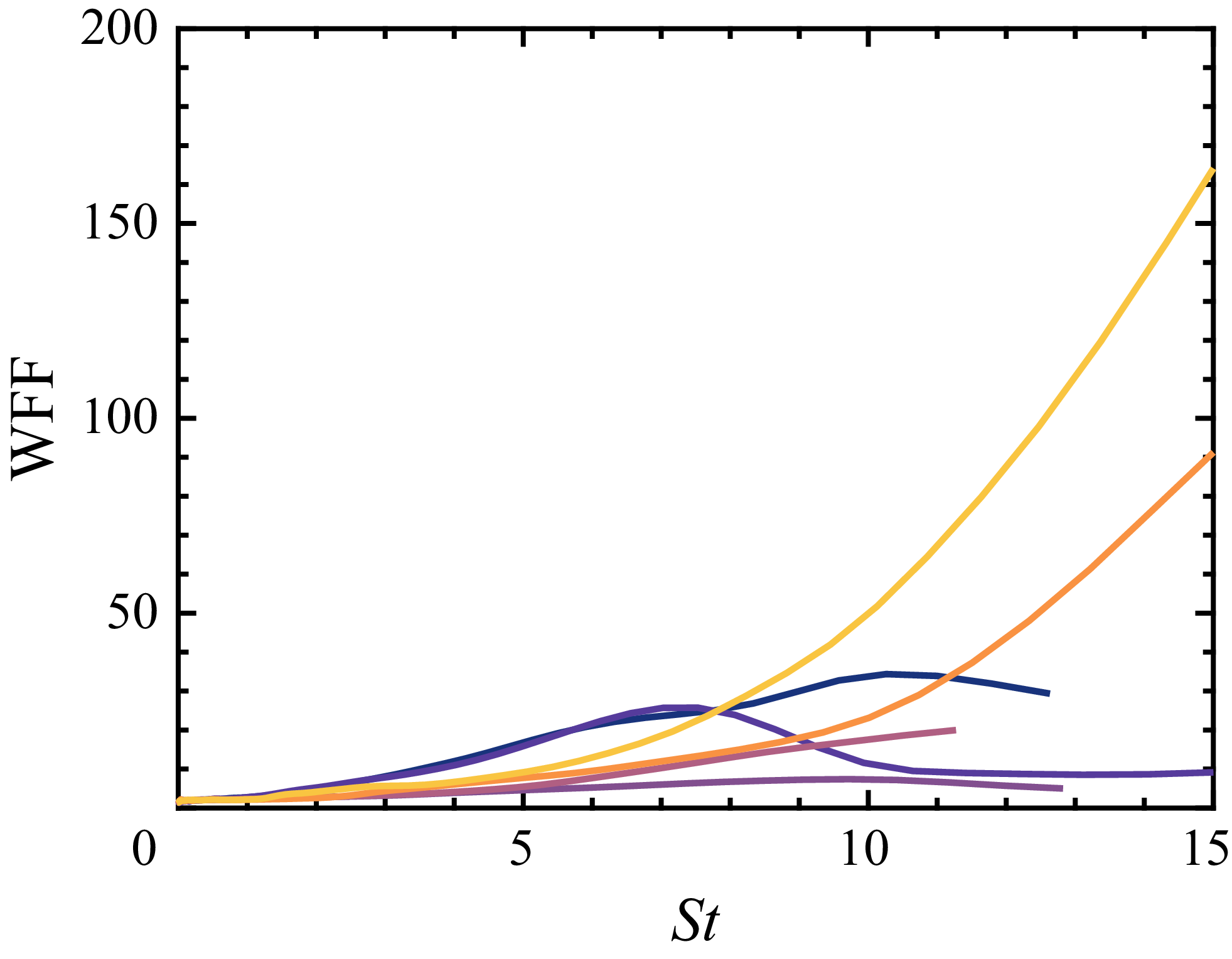
in the high-frequency range. The measure of local intermittency seems to be dominated by the high-frequency energy burst associated with extreme events. To represent the flatness factor as a function of frequency, LIM2 can be averaged in time, obtaining the wavelet flatness factor (WFF) written as (Camussi & Bogey Reference Camussi and Bogey2021; Bernardini et al. Reference Bernardini, Della Posta, Salvadore and Martelli2023a
)
 \begin{equation} \text{WFF}(\omega )=\frac {\overline {|W(\omega ,t)|^4}}{(\overline {|W(\omega ,t)|^2})^2}. \end{equation}
As shown in figure 7, from M0 to M8 with increasing EC effects, the trend of WFFs is firstly weakening and then strengthening, consistent with the trend of overall flatness factors
 $F$
in figure 4
 $(d)$
. The reason why the IC effects significantly enhance
 $F$
is reflected in the high-frequency region where WFFs of M8H and M8Q reach much larger values. Compared with these two cases, the differences of WFFs for other cases are relatively limited.
Distributions of the WFFs. For the line legend, see table 1.

5. Conditional analysis of extreme events
It has been demonstrated that EC effects do not qualitatively change the basic feature of extreme events of WPFs, while IC effects introduce additional APNSs, thereby enhancing extreme WPFs and their intermittency. Here, for further exploring the generation mechanism of the extreme events, we propose a framework of conditional analysis aimed at identifying the coherent structures associated with extreme events and elucidating the physical mechanisms leading to extreme WPFs. Specifically, on the one hand, the volumetric conditional average on the flow field is used to identify the coherent structures responsible for extreme events (Hutchins et al. Reference Hutchins, Monty, Ganapathisubramani, Ng and Marusic2011; Cardesa et al. Reference Cardesa, Monty, Soria and Chong2019; Tong et al. Reference Tong, Dong, Lai, Yuan and Li2022). On the other hand, Poisson-equation-based pressure decomposition is utilised to theoretically split pressure fluctuations in compressible TBLs. Through this approach, the generation mechanisms of extreme WPFs can be quantitatively characterised.
5.1. Coherent structures associated with extreme events
The volumetric conditional average (Hutchins et al. Reference Hutchins, Monty, Ganapathisubramani, Ng and Marusic2011; Cardesa et al. Reference Cardesa, Monty, Soria and Chong2019) is utilised to extract the coherent structures associated with extreme events. An average box with size of
 $-300\lt \Delta x^+\lt 300$
,
 $0\lt y^+\lt 200$
and
 $-150\lt \Delta z^+\lt 150$
is used, referring to Pan & Kwon (Reference Pan and Kwon2018) and Tong et al. (Reference Tong, Dong, Lai, Yuan and Li2022). The conditional averaging is conducted by attaching the origin point of the box at each extreme event and accumulating the surrounding flow fields. At least
 $8\times 10^5$
extreme events are utilised to perform conditional averages for a specific case. Since extreme events are defined according to the threshold, an identified extreme area consists of several extreme events rather than a single one. This will inevitably lead to oversampling on a specific structure. However, as examined by Stahl et al. (Reference Stahl, Prasad, Goparaju and Gaitonde2023), such oversampling does not change the dominant structures and helps to average out small-scale random fluctuations and smooth the evolution of coherent structures. The conditional averages are computed based on extremely positive and negative events. Hereafter, the conditionally averaged quantity is then denoted as
 $\left \langle \bullet \right \rangle$
.
Figure 8 shows the slices of conditionally averaged WPFs. For all cases, the regions belonging to extreme fluctuations, which are circled in white, have the shape of spots rather than the elongated streaks observed for extreme wall shear stress. From M0 to M8 in figure 8
 $(a{-}c)$
, the EC effects do not change the basic pattern of extreme WPFs. For extremely positive events, the extreme WPF spot is located downstream of a negative area with a V-shaped edge. The situation for extremely negative events is opposite, with the extreme WPF spot upstream of a positive area with a V-shaped edge. Implementing wall-cooling effects for M8H and M8Q in figures 8
 $(d)$
and 8
 $(e)$
, IC effects change the basic pattern of extreme WPFs by introducing additional strong spots with opposite signs upstream or downstream of the extreme spot. This alternating characteristic reminds us of the APNSs observed in figure 3. The significantly distinct patterns of extreme WPFs also imply the presence of different coherent structures associated with extreme events.
Slices of conditionally averaged WPFs based on extremely positive events (left-hand column) and extremely negative events (right-hand column) for cases
 $(a)$
M0,
 $(b)$
M4,
 $(c)$
M8,
 $(d)$
M8H and
 $(e)$
M8Q. The regions belonging to extreme fluctuations are circled in white.

Conditionally averaged fluctuation fields based on extremely positive events for cases
 $(a)$
M0,
 $(b)$
M8,
 $(c)$
M8H and
 $(d)$
M8Q. The high-/low-speed structures are displayed by the isosurfaces of streamwise velocity
 $u$
flooded by wall-normal velocity
 $v$
(positive/negative in red/blue), the vortex structures are displayed by the isosurfaces of the
 $Q$
-criterion flooded by streamwise vorticity
 $\omega _x$
(positive/negative in white/black) and the dilatational structures are displayed by isosurfaces of positive/negative dilatation
 $\theta$
flooded by itself (positive/negative in bright red/blue). A representative
 $x{-}y$
panel of streamwise velocity
 $u$
at
 $\Delta z^+=0$
and a
 $y{-}z$
panel of spanwise velocity
 $w$
at
 $\Delta x^+=0$
are shifted aside for clearer observation.

The conditionally averaged fluctuation fields based on extremely positive events are three-dimensionally visualised by the isosurfaces of velocity, vortex and dilatation structures along with two panels shifted aside in figure 9. For more comprehensive observation, the side and top views are presented simultaneously. For M0 in figure 9
 $(a)$
, the main flow organisation is that a high-speed structure (
 $u^{\prime \prime }\gt 0$
) with the shape of a teardrop rear-ends the downstream near-wall low-speed streak (
 $u^{\prime \prime }\lt 0$
). The extreme event located at the origin point lies directly beneath the rear-end process. The flow organisation agrees well with that in an incoming TBL of shock wave–boundary layer interactions (Limei et al. Reference Limei, Yuan, Dong, Li and Tong2024). According to the isosurfaces of the
 $Q$
-criterion flooded by streamwise vorticity
 $\omega _x$
in greyscale, two pairs of counter-rotating quasi-streamwise vortices, which are arranged along the streamwise direction, are identified. The velocity structures are located between the vortex pairs. The upstream one induces sweep motions (
 $v^{\prime \prime }\lt 0$
) and transports high momentum from the outer to the inner layer, which facilitates the formation of the high-speed structures. In contrast, the downstream one has correspondingly opposite signs of
 $\omega _x$
. Similarly, it induces ejection motions (
 $v^{\prime \prime }\gt 0$
), resulting in low-speed structures. Due to the weak compressibility in M0, the fluid is evacuated from the spanwise direction to both sides, as indicated by the divergent spanwise velocity
 $w^{\prime \prime }$
shown in the shifted panel from
 $\Delta x^+=0$
. Thus, almost no dilatation structure can be observed in the conditionally averaged field. On increasing Mach number in figure 9
 $(b{-}d)$
, the EC effects do not change the overall flow organisation consisting of high-speed structures rear-ending low-speed streaks and the associated counter-rotating vortex pairs. The major difference is that the EC effects weaken the high-speed structure and strengthen the low-speed streaks. Moreover, the divergent spanwise velocities are also suppressed, leading to the near-wall alternating dilatation structures. An expansion motion is upstream of a compression motion, with the extreme event located between them. For wall-cooling cases M8H and M8Q in figures 9
 $(c)$
and 9
 $(d)$
, IC effects change the basic flow organisations in that the rear-ending process is absent, and the dilatation structures are highly enhanced with shapes changed to that of typical APNSs. Especially for M8Q, the extreme event is mainly associated with an elongated low-speed streak, which is consistent with the property that an APNS tends to occur embedded in the near-wall low-speed streak (Tang et al. Reference Tang, Zhao, Wan and Liu2020).
Slices of conditionally averaged wall-normal velocity fluctuation based on extremely positive events at
 $\Delta z^+=0$
for cases
 $(a)$
M0,
 $(b)$
M8,
 $(c)$
M8H and
 $(d)$
M8Q. The streamlines are drawn to indicate the local quadrant.

From a perspective of quadrant analysis (Wallace Reference Wallace2016), we plot slices of conditionally averaged fluctuation fields based on extremely positive events at
 $\Delta z^+=0$
in figure 10. For case M0 in figure 10
 $(a)$
, the strong
 $Q4$
motion related to sweep events occupies the whole area behind the location of the extreme events. After the origin point, the
 $Q4$
motion encounters the near-wall
 $Q2$
motion related to ejection events. The flow is lifted to gain momentum transported from the outer layer, forming the
 $Q1$
motion (outward interaction). This flow topology is consistent with the measurement of a low-speed TBL by Ghaemi & Scarano (Reference Ghaemi and Scarano2013). Even on increasing the Mach number up to that of case M8 in figure 10
 $(b)$
, strong EC effects do not significantly change the situation, except for the damped strength of the
 $Q4$
motion. For the wall-cooling cases M8H and M8Q in figures 10
 $(c)$
and 10
 $(d)$
, positive and negative fluctuations associated with APNSs dominate in the near-wall region below the white dashed lines. Intriguingly, regardless of both EC and IC effects, the topology of these quadrants is not changed above the white dashed lines.
Conditionally averaged fluctuation fields based on extremely negative events for cases
 $(a)$
M0,
 $(b)$
M8,
 $(c)$
M8H and
 $(d)$
M8Q. The high-/low-speed structures are displayed by the isosurfaces of streamwise velocity
 $u$
flooded by wall-normal velocity
 $v$
(positive/negative in red/blue), the vortex structures are displayed by the isosurfaces of the
 $Q$
-criterion flooded by the streamwise vorticity
 $\omega _x$
(positive/negative in white/black) and the dilatational structures are displayed by isosurfaces of dilatation
 $\theta$
flooded by itself (positive/negative in bright red/blue). A representative
 $x{-}y$
panel of streamwise velocity
 $u$
at
 $\Delta z^+=0$
and
 $y{-}z$
panel of spanwise velocity
 $w$
at
 $\Delta x^+=0$
are shifted aside for clearer observation.

Regarding extremely negative events, the conditionally averaged fluctuation fields are three-dimensionally visualised in figure 11 in the same manner as that of extremely positive events. For M0 in figure 11
 $(a)$
, in contrast to the extremely positive scenario, the main flow organisations become near-wall low-speed structures (
 $u^{\prime \prime }\lt 0$
) moving away from the downstream high-speed strip structures. The vortex structures identified by the
 $Q$
-criterion (
 $Q^+=2\times 10^{-4}$
) are flooded by
 $\omega _x$
in greyscale; they have an X-shaped appearance with
 $\omega _x$
for each leg in opposite sign. The vortex in a counter-rotating state facilitates the formation of low- and high-speed structures. Due to the weak compressibility in M0, fluid converges from the spanwise to the locations of extreme events as shown by
 $w^{\prime \prime }$
in the shifted panel from
 $\Delta x^+=0$
. There is no dilatation structure identified in this conditionally averaged field. With increasing Mach number in figure 11
 $(b{-}d)$
, the EC effects mainly suppress the high-speed structure, causing it to move away from the wall, while the low-speed structure is slightly enhanced. Additionally, the dilatation structures are present and enhanced with increasing EC effects. The expansion and compression motions are arranged in the streamwise direction in order, with the extreme event located at the transition point between them. For wall-cooling cases M8H and M8Q in figures 11(
 $c$
) and 11(
 $d$
), IC effects make the near-wall structure in the conditionally averaged field thoroughly become low-speed streaks. Especially for M8Q, an elongated low-speed streak is across the whole conditional average box, and high-speed structure is nearly absent. The strong dilatation structures exhibit the feature of APNSs, with more than one alternating cycle being captured.
Slices of conditionally averaged wall-normal velocity fluctuation based on extremely negative events at
 $\Delta z^+=0$
for cases
 $(a)$
M0,
 $(b)$
M8,
 $(c)$
M8H and
 $(d)$
M8Q. The streamlines are drawn to indicate the local quadrant.

The slices of conditionally averaged wall-normal velocity fluctuation based on extremely negative events at
 $\Delta z^+=0$
are shown in figure 12. For M0 in figure 12(
 $a$
), the dominating quadrants in the field are the same as those in extremely positive events, consisting of
 $Q1$
,
 $Q2$
and
 $Q4$
motions. However, the relative positions of these motions are reversed, such that
 $Q1$
motion is above
 $Q2$
motion and together follows
 $Q4$
motion. A small clockwise-rotating spanwise vortex forms near the extreme event. On increasing the Mach number to that of case M8 in figure 12(
 $b$
), the EC effects enhance
 $Q1$
motion and suppress
 $Q4$
motion. Meanwhile, they make the clockwise-rotating spanwise vortex grow significantly, with the upper edge up to
 $y^+\approx 60$
. For the wall-cooling cases M8H and M8Q in figures 12
 $(c)$
and 12
 $(d)$
, IC effects make the clockwise-rotating spanwise vortex to be lifted downstream. The near-wall region below the white dashed lines is occupied by the fluctuations mainly induced by APNSs. The topology of quadrants above the white dashed lines almost does not depend on either EC or IC effects, remaining the same as the feature in extremely positive events.
Distributions of pressure gradient
 $(({u_c}/{p_w}) ({\partial p^\prime }/{\partial x}))^+$
denoted by circles and dilatation
 $\theta ^{\prime +}$
denoted by solid lines at
 $\Delta z^+ =0$
in the conditionally averaged field for
 $(a)$
extremely positive and
 $(b)$
extremely negative events. For the line legend, see table 1.

Regarding the close link between extreme WPFs and dilatation structures, we try to interpret their relation theoretically. Extracting the mean part from the continuous equation, we write
 \begin{equation} \frac {\partial \rho ^\prime }{\partial t}+\frac {\partial (\bar {\rho }u_i^\prime +\rho ^\prime \bar {u_i})}{\partial x_i}=0. \end{equation}
Due to the no-slip isothermal wall boundary condition, the WPF is proportional to the density fluctuation at the wall, obtaining
 \begin{equation} \frac {1}{p_w}\frac {\partial p^\prime _w}{\partial t}+\theta _w^\prime =0. \end{equation}
Invoking Taylor’s hypothesis of frozen flow, i.e.
 ${\partial p^\prime }/{\partial t}\approx -u_c\partial p^\prime /\partial x$
with
 $u_c$
denoting the convection speed, it results in
 \begin{equation} \frac {u_c}{p_w}\frac {\partial p^\prime _w}{\partial x}\approx \theta _w^\prime . \end{equation}
Figure 13 displays the distributions of wall pressure gradient and dilatation at
 $\Delta z^+ =0$
in the conditionally averaged field, with
 $u_c$
estimated based on the typical convection speed of near-wall turbulent eddies
 $u_c\approx 0.6u_\infty$
(Zhang et al. Reference Zhang, Liu, Wan, Sun, Lu, Chen and Dong2024b
). Generally, the distributions of all the cases well support the relation of (5.3). Before extremely positive WPFs
 $(\Delta x^+\lt 0)$
, there are positive streamwise pressure gradients accompanied by positive dilatations. Subsequently, these values become negative after extreme events
 $(\Delta x^+\lt 0)$
, recovering WPFs back to zero. The situation for extremely negative events is similar to that for positive ones. Notably, the location of extreme events
 $\Delta x^+=0$
is the transition point of positive and negative values for both the pressure gradient and dilatation. For M8H and M8Q, it is noted that the amplitudes of the circles are slightly higher and lower than those of the solid lines for extremely positive and negative events, respectively. This implies an acoustic nature of the extreme WPFs in these two cases, characterised by convective speeds corresponding to fast and slow waves
 $u_c\approx 0.6u_\infty \pm a_w$
, where
 $a_w$
denotes the acoustic speed at the wall.
5.2. Generation mechanism responsible for extreme events
The conditionally averaged fields have effectively visualised the coherent structures associated with extreme events, providing clear insights into their characteristics. However, pressure fluctuations have the property of non-locality, which means the generation of pressure fluctuations is not merely correlated with the local structures. To further quantitatively characterise the global contribution of flow structures to extreme WPFs, we decompose pressure fluctuations according to different generation mechanisms. Based on compressible Navier–Stokes equations in a Cartesian coordinate system, take the divergence of the momentum equations and subtract the mean part from them, obtaining the equation of pressure fluctuations (Gerolymos, Sénéchal & Vallet Reference Gerolymos, Sénéchal and Vallet2007), written as
 \begin{equation} \frac {\partial ^{2} p^{\prime }}{\partial x_{i} \partial x_{i}}=\frac {\partial ^{2}}{\partial x_{i} \partial x_{j}} \tau _{i j}^{\prime }-\frac {\partial ^{2}}{\partial x_{i} \partial x_{j}}\big (2 \rho \tilde {u}_{i} u_{j}^{\prime \prime }+\rho ^{\prime } \tilde {u}_{i} \tilde {u}_{j}\big )-\frac {\partial ^{2}}{\partial x_{i} \partial x_{j}}\big (\rho u_{i}^{\prime \prime } u_{j}^{\prime \prime }-\overline {\rho u_{i}^{\prime \prime } u_{j}^{\prime \prime }}\big )+\frac {\partial ^{2} \rho ^{\prime }}{\partial t^{2}}, \end{equation}
where
 $\tau _{i j}$
is the viscous stress tensor. According to the physical meaning of the source terms on the right-hand side of (5.4), the pressure fluctuation in compressible flow can be decomposed into several components (Yu et al. Reference Yu, Xu and Pirozzoli2020; Zhang et al. Reference Zhang, Wan, Liu, Sun and Lu2022), i.e.
 $p^\prime =p_r+p_s+p_\tau +p_c+p_h$
. These pressure components, respectively, satisfy
 \begin{align} \frac {\partial ^{2} p_{r}}{\partial x_{i} \partial x_{i}}=&-2 \frac {\partial \tilde {u}_{i}}{\partial x_{j}} \frac {\partial \rho u_{j}^{\prime \prime }}{\partial x_{i}}, \end{align}
 \begin{align} \frac {\partial ^{2} p_{s}}{\partial x_{i} \partial x_{i}}=&-\frac {\partial ^{2}}{\partial x_{i} \partial x_{j}}\big (\rho u_{i}^{\prime \prime } u_{j}^{\prime \prime }-\overline {\rho u_{i}^{\prime \prime } u_{j}^{\prime \prime }}\big ), \end{align}
 \begin{align} \frac {\partial ^{2} p_{\tau }}{\partial x_{i} \partial x_{i}}=&\;\frac {\partial ^{2} \tau _{i j}^{\prime }}{\partial x_{i} \partial x_{j}}, \end{align}
 \begin{align} \frac {\partial ^{2} p_{c}}{\partial x_{i} \partial x_{i}}=&\;\frac {\partial ^{2} \rho ^{\prime }}{\partial t^{2}}-\frac {\partial ^{2}}{\partial x_{i} \partial x_{j}}\big (2 \rho \tilde {u}_{i} u_{j}^{\prime \prime }+\rho ^{\prime } \tilde {u}_{i} \tilde {u}_{j}\big )+2 \frac {\partial \tilde {u}_{i}}{\partial x_{j}} \frac {\partial \rho u_{j}^{\prime \prime }}{\partial x_{i}}, \end{align}
 \begin{align} \frac {\partial ^{2} p_{h}}{\partial x_{i} \partial x_{i}}=&\;0. \end{align}
The first two components
 $p_r$
and
 $p_s$
are so-called rapid and slow pressures similar to those in incompressible flow (Kraichnan Reference Kraichnan1956) according to their response speed to the change of mean flow. They are caused by linear mean flow–turbulence interactions and nonlinear turbulence–turbulence interactions, respectively. The viscous pressure
 $p_\tau$
is associated with the contribution of the viscous stress. The compressible pressure
 $p_c$
is mainly caused by compressibility, which is the efficient representation of the essential nature of compressibility effects on the pressure statistics (Sarkar Reference Sarkar1992; Foysi et al. Reference Foysi, Sarkar and Friedrich2004; Tang et al. Reference Tang, Zhao, Wan and Liu2020). Finally, the harmonic pressure
 $p_h$
is introduced to indicate the contribution of streamwise boundary conditions (Pope Reference Pope2000), which should be negligible far away from the streamwise boundary. Given the DNS data, all the source terms of pressure components can be obtained by post-processing. Then, the Poisson equations of pressure components are numerically solved by the Fourier–Galerkin scheme in a subdomain of the computational domain.
Instantaneous distributions of pressure fluctuation and its components in the wall unit.

Taking M0, M8 and M8H as examples, we show the instantaneous distributions of pressure fluctuation and its components in figure 14. Observing the characteristic peaks in the original pressure fluctuation fields
 $p^{\prime +}$
, the corresponding imprints can be found in certain pressure components. For M0, the dominating components are rapid pressure
 $p^{\prime +}_r$
and slow pressure
 $p^{\prime +}_s$
, which have the same order of amplitude as that of
 $p^{\prime +}$
. As a result of linear interactions of mean flow and turbulence, the
 $p^{\prime +}_r$
field seems to have relatively large-scale patterns arranged in the spanwise direction. The
 $p^{\prime +}_s$
field appears to be dominated by small-scale turbulent eddies, representing the outcome of nonlinear interactions of turbulence. In the wavenumber spectrum, the characteristic wavelength of
 $p^{\prime +}_s$
with energy peak is shorter than that of
 $p^{\prime +}_r$
(Zhang et al. Reference Zhang, Wan, Liu, Sun and Lu2022). The amplitudes of viscous pressure
 $p^{\prime +}_\tau$
and compressible pressure
 $p^{\prime +}_c$
are very small. According to the streamwise and spanwise planes,
 $p^{\prime +}_\tau$
only concentrates in the viscous sublayer where the viscous stress plays a dominant role. The field of
 $p^{\prime +}_c$
shows large-scale patterns in the whole domain. The acoustic waves radiating out of the boundary layer are captured by
 $p^{\prime +}_c$
. For M8, the qualitative properties of
 $p^{\prime +}_r$
,
 $p^{\prime +}_s$
and
 $p^{\prime +}_\tau$
are not influenced by strong EC effects. The field of
 $p^{\prime +}_c$
representing the acoustic activity is significantly enhanced to an amplitude comparable to that of
 $p^{\prime +}_r$
and
 $p^{\prime +}_s$
. For M8H, APNSs induced by IC effects mainly modify the fields of
 $p^{\prime +}_\tau$
and
 $p^{\prime +}_c$
. There are some negative regions associated with APNSs in the
 $p^{\prime +}_\tau$
field. The amplitude of
 $p^{\prime +}_c$
is further amplified with some local extreme values as the imprint of APNSs.
Joint p.d.f.s of extreme WPFs and their components for
 $(a{,} b{,} e{,} f)$
extremely positive events and
 $(c{,} d{,} g{,} h)$
extremely negative events:
 $(a{,} c)$
rapid pressure
 $p_r^\prime$
,
 $(b{,}d )$
slow pressure
 $p_s^\prime$
,
 $(e{,} g)$
viscous pressure
 $p_\tau ^\prime$
and
 $(f{,}h)$
compressible pressure
 $p_c^\prime$
. For the line legend, see table 1, and the isolines denote the values of 1, 3 and 5, respectively. The dashed lines denote the perfectly correlated linear relation.

To systematically illustrate the dependence of the quantitative contribution of generation mechanisms to extreme events on compressibility effects, we plot joint p.d.f.s of extreme WPFs and their components for all the cases in figure 15. Regarding the rapid pressure
 $p_r^\prime$
shown in figure 15
 $(a)$
, for cases from M0 to M8 as indicated by the inclined arrow, the isolines of joint p.d.f.s are mainly located in the positive region, which benefits the generation of extremely positive events. The EC effects make the isolines move negatively, slightly decreasing the contribution of
 $p_r^\prime$
. However, for wall-cooling cases M8H and M8Q, the decrease induced by IC effects is so significant that the isolines are transported to even negative regions. Under this condition, the interaction of mean flow and turbulence tends to resist the generation of extreme events. For extremely negative events in figure 15
 $(c)$
, the tendency of compressibility effects on the contribution of
 $p_r^\prime$
to extreme pressure is the same: they decrease, but slightly due to EC effects and significantly due to IC effects. For slow pressure
 $p_s^\prime$
in extremely positive and negative events shown in figures 15
 $(b)$
and 15
 $(d)$
, respectively, the influence of compressibility effects on the distributions of joint p.d.f.s is quite limited. Even for M8Q with strong IC effects, the displacement of isolines is still relatively small. Because
 $p_s^\prime$
originates from nonlinear turbulence interactions and is primarily associated with small-scale turbulence, the present result drops the hint that the normalised behaviour of small-scale turbulence inducing pressure fluctuations in TBLs is influenced by compressible effects very weakly. This point is qualitatively consistent with the finding of Hasan et al. (Reference Hasan, Costa, Larsson, Pirozzoli and Pecnik2025) that the small scales of turbulence, reflected by the dissipation of turbulent kinetic energy, are almost not affected by IC effects. For viscous pressure
 $p_\tau ^\prime$
in figures 15
 $(e)$
and 15
 $(g)$
, compressibility effects on distributions of joint p.d.f.s do not differ for extremely positive and negative events. The isolines of cases from M0 to M8 collapse with each other very well, indicating that the contribution of viscous stress fluctuations does not depend on EC effects. For wall-cooling cases M8H and M8Q, IC effects make the distribution of isolines wider and flatter and shift negatively regardless of extremely positive or negative events. This is because APNSs can induce the negative region of
 $p_\tau ^\prime$
as shown in figure 14. For compressible pressure
 $p_c^\prime$
in figures 15
 $(f)$
and 15
 $(h)$
, both EC and IC effects play an essential role in modifying the contribution of compressibility to extreme WPFs. The isolines of joint p.d.f.s for M0 are narrow and elongated and located near 0. The EC effects give broad and flat isolines and shift them positively and negatively for extremely positive and negative events, respectively. The impact of IC effects exhibits qualitatively similar characteristics, yet at a significantly intensified level. Especially for M8Q, the probability of a point exceeding the perfectly correlated linear relation denoted by the dashed lines is considerable. In that situation, the amplitude of the compressible component
 $p_c^\prime$
can be much larger than that of the extreme WPF itself. As reported by Zhang et al. (Reference Zhang, Wan, Liu, Sun and Lu2022), when IC effects are primary, the interactions between
 $p_r^\prime$
and
 $p_c^\prime$
become non-negligible with a negative value, implying that
 $p_r^\prime$
and
 $p_c^\prime$
are negatively correlated.
Contributions of pressure components to extreme events for
 $(a{,} b)$
extremely positive events and
 $(c{,} d)$
extremely negative events:
 $(a{,} c)$
quasi-adiabatic
 $T_w/T_r=1$
cases and
 $(b{,} d)$
 $M=8$
cases. The symbols from dark to light denote the results of
 $\varepsilon =0.1\,\%,\ 1\,\%$
and
 $10\,\%$
, respectively. The dashed lines denote linear relations based on fittings according to the result of
 $\varepsilon =1\,\%$
.

To describe the contributions of each generation mechanism to extreme WPFs concisely and globally, we calculate the conditionally averaged value of
 $\langle p^\prime _i/p^\prime _w \rangle$
, where
 $p^\prime _i$
denotes a certain pressure component. This conditional value, as depicted in figure 16, quantitatively measures the composition of extreme WPFs. For a single pressure component in each case, three symbols are displayed with colours from dark to light, representing the results based on thresholds satisfying
 $\varepsilon =0.1\,\%,\ 1\,\%$
and
 $10\,\%$
, respectively. For extremely positive and negative events of cases from M0 to M8 in figures 16
 $(a)$
and 16
 $(c)$
, the EC effects suppress the contributions of
 $p^\prime _r$
and
 $p^\prime _s$
and enhance the contribution of
 $p^\prime _c$
. The tendency can be well reflected by the dashed lines denoting linear relations based on fittings according to the result of
 $\varepsilon =1\,\%$
. The decreasing speed of
 $p^\prime _r$
with
 $M$
is faster than that of
 $p^\prime _s$
. The contribution of
 $p^\prime _\tau$
is relatively limited, about 0.06, and remains unaffected by EC effects, whereas the contribution of
 $p^\prime _h$
remains zero. For cases of
 $M=8$
shown in figures 16
 $(b)$
and 16
 $(d)$
, the most notable impact of IC effects is that they significantly increase the contribution of
 $p^\prime _c$
up to and exceeding 1.5, and also significantly decrease the contribution of
 $p^\prime _r$
to negative values of near −1. Given the high amplitude of WPFs induced by APNSs and the dilatational nature of APNSs, the dominating contribution of
 $p^\prime _c$
is expected. Meanwhile, when APNSs occur, the coupling between
 $p^\prime _r$
and
 $p^\prime _c$
becomes strong. In comparison, the IC effects on the contributions of
 $p^\prime _s$
and
 $p^\prime _\tau$
are much weaker. Specifically, the IC effects decrease and increase the contribution of
 $p^\prime _\tau$
in extremely positive and negative events, respectively. It should be highlighted that when modifying the thresholds making
 $\varepsilon$
change from
 $0.1\,\%$
to
 $10\,\%$
, spanning two orders of magnitude, the overall tendency of compressible effects remains qualitatively unchanged, despite some noticeable scatter appearing under IC effects.
6. Conclusion
The generation mechanisms of extreme WPF events in TBLs and the impact of compressibility effects are investigated systematically. The intermittency property of WPFs is illustrated by single-point statistics and wavelet analysis. Then, the coherent turbulent structures associated with extreme events are identified by volumetric conditional average. Further, the contributions of each physical mechanism generating pressure fluctuations to extreme events are quantified by means of the Poisson-equation-based pressure decomposition. The primary findings are summarised as follows.
Firstly, compressibility effects at different levels, encompassing both EC and IC effects, are achieved by increasing the Mach number and decreasing the wall temperature. The EC effects, associated with variable properties of mean thermodynamic quantities, only weakly affect the intermittency of WPFs. In contrast, the IC effects, associated with changes in fluid volume in response to pressure fluctuations, significantly enhance the intermittency, particularly as manifested in the high-frequency range. This phenomenon is correlated with the occurrence of travelling wave-packet-like dilatational APNSs with a fine characteristic length scale of
 $\lambda _x^+\approx 100$
.
Secondly, volumetrically conditional averages are performed based on extreme WPF events, which correspond to the top
 $\varepsilon =1\,\%$
of the most intense events. At low Mach numbers, extremely positive events are induced by a high-speed structure from the outer layer rear-ending a near-wall low-speed streak, and extremely negative events are associated with an inclined X-shaped vortex, which induces a near-wall low-speed structure following a downstream high-speed structure extending to the outer layer. The EC effects do not change these flow organisations but enhance the dilatation structures induced by them. However, when IC effects are present, the coupled presence of high- and low-speed structures disappears in the conditionally averaged field, and the extremely positive and negative events are primarily associated with the strong expansion and compressible motions by APNSs, respectively. Moreover, the relation between the streamwise gradient of pressure
 $\partial p_w^\prime /\partial x$
and the dilatation at the wall
 $\theta _w^\prime$
is derived and verified by the conditionally averaged field, which shows that they are in proportional scaling with the ratio of
 $u_c/p_w$
.
Finally, the Poisson-equation-based pressure decomposition is utilised to split the original pressure fluctuations into rapid, slow, viscous and compressible pressure components, which are generated by turbulence–mean flow interactions, turbulence–turbulence interactions, viscous stress and compressibility effects, respectively. Then, the composition of extreme WPFs can be quantified by conditionally sampling the pressure components. The contributions of slow and viscous pressure to extreme WPFs are almost not affected by EC effects and weakly affected by IC effects, probably because these two components mainly represent the behaviour of small-scale turbulence. Compressibility effects monotonically suppress the contribution of rapid pressure and enhance the contribution of compressible pressure as expected. Furthermore, the influence of IC effects is much more significant than that of EC effects. It is worth noting that when we modify the thresholds of extreme events and make
 $\varepsilon$
change from
 $0.1\,\%$
to
 $10\,\%$
, spanning two orders of magnitude, the overall trend of the composition of extreme WPFs remains nearly unchanged.
It is worth mentioning that the present conclusions are drawn from analysing the TBL data encompassing a wide range of Mach numbers
 $0.5\leqslant Ma \leqslant 8.0$
and wall-to-recovery temperature ratios
 $0.25 \leqslant T_w/T_r \leqslant 1.0$
. A key limitation, however, lies in the Reynolds number, which is fixed at
 $Re_\tau \approx 630$
. Thus, the applicability of these conclusions may be limited in cases with significantly higher Reynolds numbers.
Acknowledgements
The numerical computations were performed at Hefei Advanced Computing Center.
Funding
This work was supported by the National Natural Science Foundation of China under grant nos. 12388101, 12402258, 12322210, 92252202 and 12172351.
Declaration of interests
The authors report no conflict of interest.