1 Introduction
Vortex-induced vibration (VIV) of structures is encountered in a variety of engineering situations, such as for flows past offshore structures, bridges, heat exchangers, aircraft, pipelines and other hydrodynamic applications. The practical significance of VIV has led to numerous studies focusing on understanding the underlying physics, including the comprehensive reviews by Bearman (Reference Bearman1984), Blevins (Reference Blevins1990), Sarpkaya (Reference Sarpkaya2004), Williamson & Govardhan (Reference Williamson and Govardhan2004), Païdoussis, Price & De Langre (Reference Païdoussis, Price and De Langre2010) and Naudascher & Rockwell (Reference Naudascher and Rockwell2012). Most of the previous studies, however, were focused on two-dimensional (2-D) bluff bodies like cylinders. There are relatively fewer studies on the VIV of elastically mounted or tethered spheres despite their ubiquitous practical significance, such as marine buoys, underwater mines, other offshore structures and tethered or towed spheroidal objects. Govardhan & Williamson (Reference Govardhan and Williamson1997), Williamson & Govardhan (Reference Williamson and Govardhan1997) and Jauvtis, Govardhan & Williamson (Reference Jauvtis, Govardhan and Williamson2001) were among the first to report on the VIV response of a sphere identifying three fundamental modes of vibration, namely modes I, II and III. Since then, a number of systematic studies have investigated the VIV response of spheres, e.g. Pregnalato (Reference Pregnalato2003), Govardhan & Williamson (Reference Govardhan and Williamson2005), van Hout, Krakovich & Gottlieb (Reference van Hout, Krakovich and Gottlieb2010), Behara, Borazjani & Sotiropoulos (Reference Behara, Borazjani and Sotiropoulos2011), Krakovich, Eshbal & van Hout (Reference Krakovich, Eshbal and van Hout2013), Lee, Hourigan & Thompson (Reference Lee, Hourigan and Thompson2013), Behara & Sotiropoulos (Reference Behara and Sotiropoulos2016) and Sareen et al. (Reference Sareen, Zhao, Lo Jacono, Sheridan, Hourigan and Thompson2018a ).
Large-amplitude vibration caused by VIV over a wide range of Reynolds number is a common cause of serious structural fatigue and damage, which has led to a plethora of research studies focusing on suppressing VIV over last four decades. For this reason, several active and passive control methods have been studied previously for 2-D bluff bodies. Choi, Jeon & Kim (Reference Choi, Jeon and Kim2008) provide a review of various control methods employed for flow over bluff bodies. Although passive control methods do not consume external energy and are fairly insensitive to changes in the flow direction, it tends to be difficult to dramatically reduce VIV, and the drag often increases. In contrast, active control methods such as moving-surface boundary-layer control (MSBC) (Mittal Reference Mittal2001) and windward suction leeward blowing (WSLB) (Dong, Triantafyllou & Karniadakis Reference Dong, Triantafyllou and Karniadakis2008) reduce VIV to a much lower level; however, the efficacy of both these active methods depends on the flow direction.
The control of VIV by rotary motion has received increased attention recently due to its insensitivity to flow direction, efficacy over a broader range of flow parameters and the greater extent of VIV reduction. A recent experimental study by Sareen et al. (Reference Sareen, Zhao, Lo Jacono, Sheridan, Hourigan and Thompson2018a ) reported suppression of VIV of a sphere by means of an imposed transverse rotation for a wide range of Reynolds numbers and reduced velocities. They reported a reduction in the strength of the vortex street, which can be associated with a reduction of the transverse force acting on the sphere. VIV can also be suppressed by forced sinusoidal rotary oscillations of the bluff body, to prohibit the phenomenon of resonance or ‘lock-in’ by deviating the vortex shedding frequency from the natural frequency of the system towards the forcing frequency (also known as ‘lock-on’).
This approach has been extensively investigated on a fixed cylinder over the last four decades. Taneda (Reference Taneda1978) was the first to examine this experimentally for a rotary oscillating cylinder, and reported the disappearance of vortex shedding for very high forcing frequencies. Later, Tokumaru & Dimotakis (Reference Tokumaru and Dimotakis1991) reported a drag reduction of up to 80 % for a certain range of forcing frequencies and amplitudes of sinusoidal rotary oscillations. This pioneering study inspired a number of systematic numerical studies aimed at understanding this wake control and the underlying dynamics, such as Tokumaru & Dimotakis (Reference Tokumaru and Dimotakis1991), Lu & Sato (Reference Lu and Sato1996), Chou (Reference Chou1997), Baek & Sung (Reference Baek and Sung2000), Mahfouz & Badr (Reference Mahfouz and Badr2000), Cheng, Chew & Luo (Reference Cheng, Chew and Luo2001), Shiels & Leonard (Reference Shiels and Leonard2001), Choi, Choi & Kang (Reference Choi, Choi and Kang2002), Lee & Lee (Reference Lee and Lee2006) and Kumar et al. (Reference Kumar, Lopez, Probst, Francisco, Askari and Yang2013). It is known for the case of a fixed cylinder that for a certain range of forcing frequency ratios encompassing the natural frequency of the system, the vortex shedding locks to the forcing frequency, leading to the ‘lock-on’ phenomenon (Chou Reference Chou1997; Baek & Sung Reference Baek and Sung2000). The state is accompanied by a significant drag reduction (Tokumaru & Dimotakis Reference Tokumaru and Dimotakis1991; Lu & Sato Reference Lu and Sato1996; Chou Reference Chou1997). The lock-on region widens with increasing rotational speed (Mahfouz & Badr Reference Mahfouz and Badr2000). The boundaries of lock-on and non-lock-on regions are associated with the modulation of the drag, lift and velocity (Choi et al. Reference Choi, Choi and Kang2002), and the non-lock-on regions exhibit quasi-periodicity (Baek & Sung Reference Baek and Sung2000). Several studies have focused on understanding the underlying dynamics. It was found that the lock-on region is associated with enhanced separation and vortex coalescence in the wake (Cheng et al. Reference Cheng, Chew and Luo2001; Shiels & Leonard Reference Shiels and Leonard2001; Lee & Lee Reference Lee and Lee2006). The experimental investigation by Thiria, Goujon-Durand & Wesfreid (Reference Thiria, Goujon-Durand and Wesfreid2006) also revealed that the phase lag between the vortex shedding and the rotary motion of the cylinder effectively gives either a constructive or destructive contribution to the wake, leading to a global decrease or increase in fluctuations in the wake.
Recently, Du & Sun (Reference Du and Sun2015) investigated numerically the potential of rotary oscillations to suppress VIV of an elastically mounted cylinder at
 $Re=350$
. They found ‘lock-on’ for the elastically mounted cylinder, which led to switching of vortex shedding from the natural frequency to the forcing frequency, inhibiting resonance or VIV. They observed effective control only for large enough velocity ratios, and the lock-on regime became narrower with an increase in reduced velocity. They observed no significant reduction in the strength of vortices in the wake.
The papers discussed so far report on rotational control of 2-D bluff bodies. However, there do not appear to be studies investigating the potential of rotary oscillations in wake control for 3-D bluff bodies, such as spheres. However, a sphere is the most basic 3-D body shape; certainly the one with the most symmetry, and clearly spheres can undergo significant amplitude VIV. A sphere provides a starting framework to comprehend VIV control of more complex three-dimensional bluff bodies. The current study aims at producing an understanding of the effect of imposed rotary oscillations on the VIV response of a sphere for a wide range of forcing and flow parameters. One question to be addressed is whether similar features (as discussed above for a fixed cylinder) are exhibited in the case of an elastically mounted sphere. Specifically, this study addresses the following fundamental questions: Is ‘lock-on’ also observed for a sphere exhibiting a 3-D wake? If so, how does the lock-on range depend on various forcing and flow parameters? How does this phenomenon affect the 3-D wake structures of the flow past a sphere?
The outline of the article is as follows. The experimental methodology for the current experiments is detailed in § 2. The VIV response of a non-rotating oscillating sphere is briefly presented in § 3. Section 4.1 discusses in detail the effect of frequency ratio on the VIV response of a sphere, followed by § 4.2 on the effect of velocity ratio. § 4.3 focuses on the effect of the reduced velocity on the VIV response. Section 5 discusses the effect on the wake structures, and finally § 6 draws conclusions, and summarises the important findings and significance of the current study. To be clear, in this article, if the vibrations are locked to the natural frequency, the phenomenon is termed ‘lock-in’ or ‘resonance’, and if they are locked to the forcing frequency instead, it is termed ‘lock-on’ or, in this case,‘rotary lock-on’.
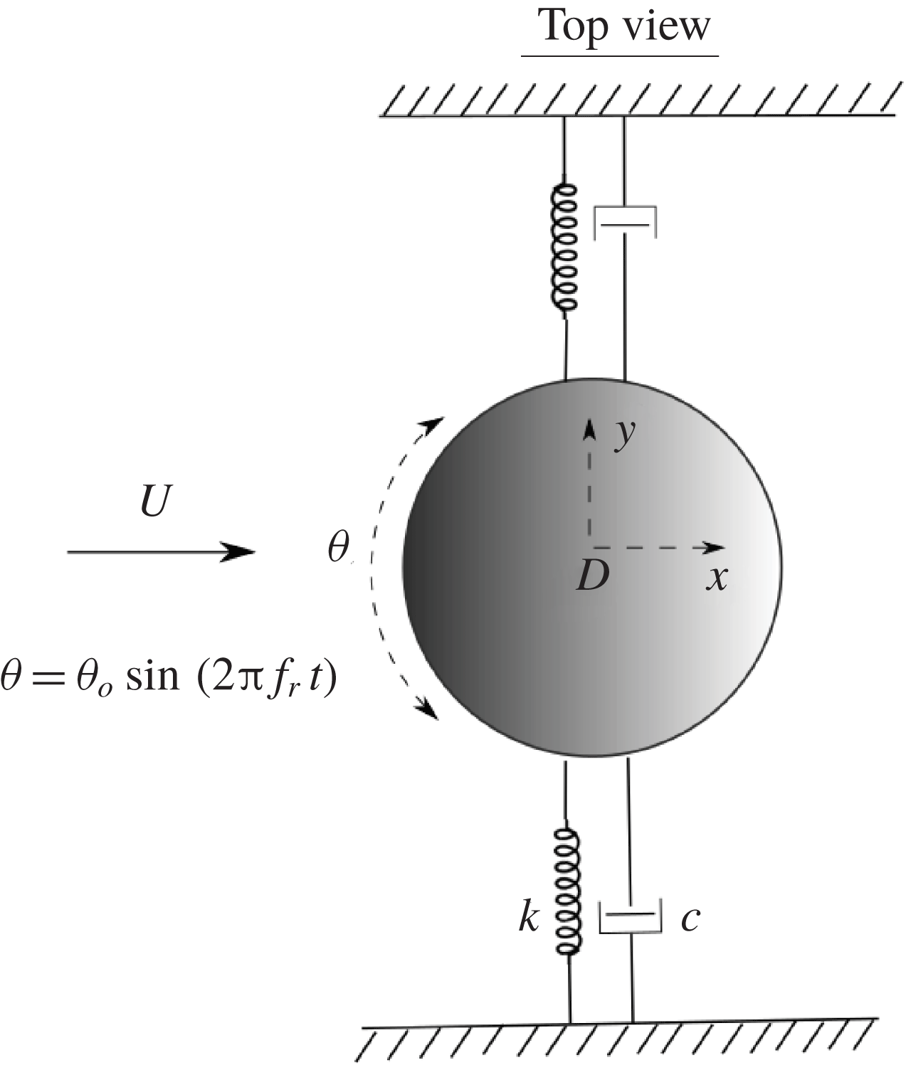
Definition sketch for the transverse vortex-induced vibration of a sphere undergoing forced rotary oscillations. The hydro-elastic system is simplified as a one-degree-of-freedom (1-DOF) system constrained to move only in the cross-flow direction. The axis of rotation (
 $z$
) is transverse to both the flow direction (
 $x$
-axis) and the oscillation axis (
 $y$
-axis). Here,
 $U$
is the free-stream velocity,
 $k$
the spring constant,
 $D$
the sphere diameter,
 $c$
the structural damping and
 $\unicode[STIX]{x1D703}$
the imposed angular displacement.

2 Experimental method
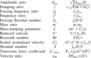
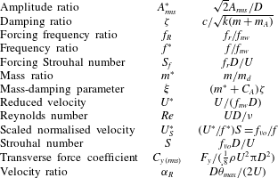
Non-dimensional parameters used in this study. In this table:
 $A_{rms}$
is the root-mean-square (r.m.s.) value of the vibration amplitude in the
 $y$
direction;
 $D$
is the sphere diameter;
 $f$
is the body oscillation frequency;
 $f_{r}$
is the frequency of the imposed rotary oscillation; and
 $f_{nw}$
is the natural frequency of the system in quiescent water. In addition,
 $m$
is the total oscillating mass;
 $c$
is the structural damping factor with
 $k$
the spring constant;
 $U$
is the free-stream velocity;
 $\unicode[STIX]{x1D708}$
is the kinematic viscosity;
 $m_{A}$
denotes the added mass, defined by
 $m_{A}=C_{A}m_{d}$
, where
 $m_{d}$
is the mass of the displaced fluid and
 $C_{A}$
is the added mass coefficient (0.5 for a sphere);
 $\dot{\unicode[STIX]{x1D703}}_{max}$
= maximum angular velocity of the sphere;
 $f_{vo}$
is the vortex shedding frequency of a fixed body and
 $F_{y}$
is the fluid force acting on the sphere in the transverse direction.
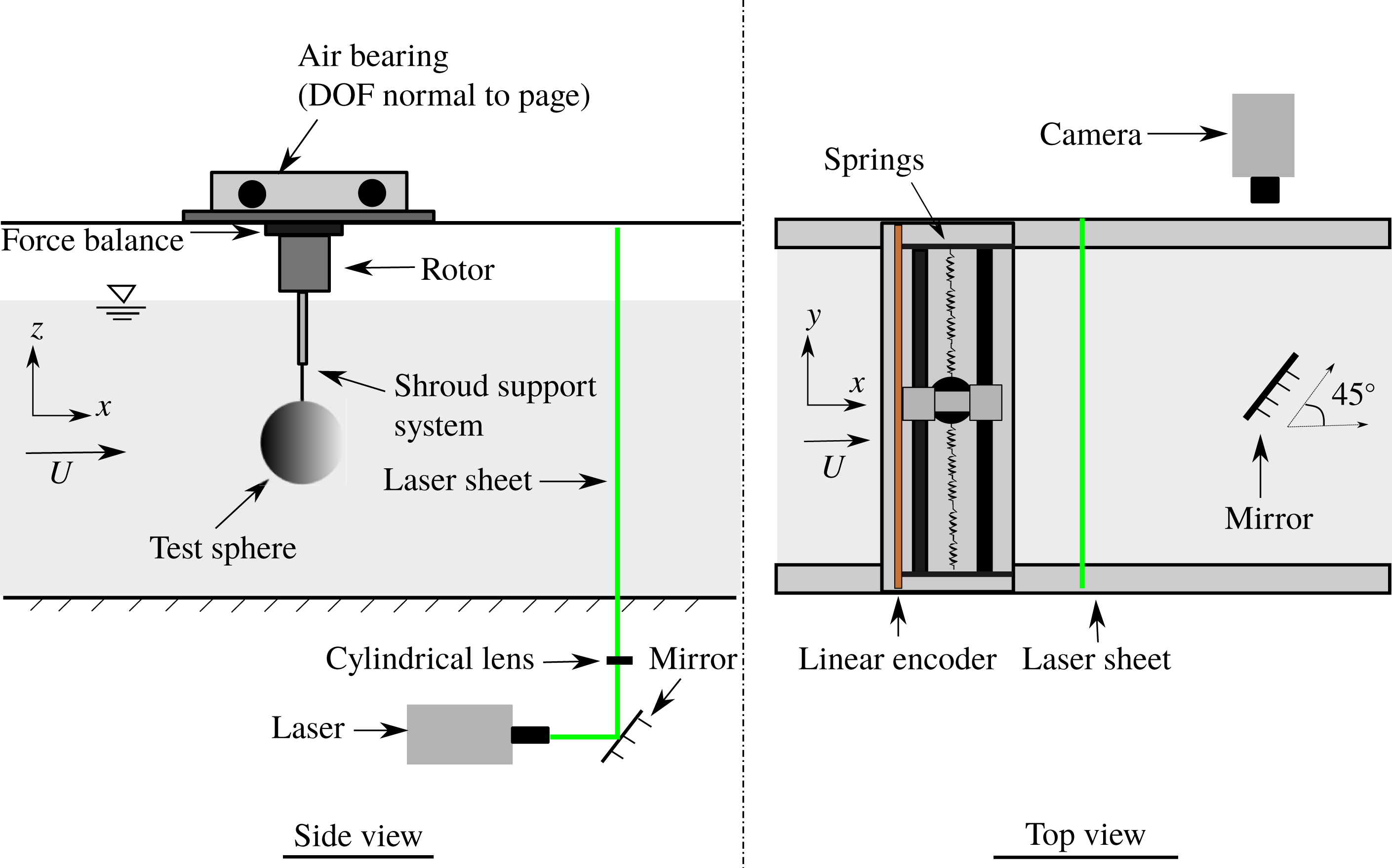
A schematic showing the experimental arrangement of the current fluid–structure interaction problem is presented in figure 1. The sphere is elastically mounted in the direction transverse to the incoming flow. The axis of the sinusoidal rotary oscillations imposed on the sphere is transverse to the flow direction and the free vibration axis.
The two important parameters characterising the rotary oscillation motion of the sphere are
 $f_{R}$
and
 $\unicode[STIX]{x1D6FC}_{R}$
. Here,
 $f_{R}$
is the forcing frequency ratio, expressed as the ratio of forcing frequency,
 $f_{r}$
, and the natural frequency of the system,
 $f_{nw}$
, as
 $$\begin{eqnarray}f_{R}=f_{r}/f_{nw}.\end{eqnarray}$$
Alternatively, sometimes the non-dimensional forcing Strouhal number is used to characterise the forcing
 $$\begin{eqnarray}S_{f}=\frac{f_{r}D}{U}.\end{eqnarray}$$
The other key parameter,
 $\unicode[STIX]{x1D6FC}_{R}$
, is the forcing velocity ratio expressed as the ratio of the maximum tangential velocity of the sphere surface and the free-stream velocity
 $U$
as
 $$\begin{eqnarray}\unicode[STIX]{x1D6FC}_{R}=\frac{D\dot{\unicode[STIX]{x1D703}}_{max}}{2U},\end{eqnarray}$$
where
 $\dot{\unicode[STIX]{x1D703}}_{max}$
is the maximum angular velocity of the sphere. All other relevant non-dimensional parameters for the current study are listed in table 1.
The governing equation of motion describing the cross-flow motion of the sphere can be written as
 $$\begin{eqnarray}m\ddot{y} +c{\dot{y}}+ky=F_{y},\end{eqnarray}$$
where
 $F_{y}$
is the fluid force in the transverse direction,
 $m$
is the total oscillating mass of the system,
 $y$
is the displacement in the transverse direction,
 $c$
is the structural damping of the system and
 $k$
is the spring constant. Using the above equation, the total fluid force in the transverse direction can be calculated with the knowledge of the directly measured displacement, and its time derivatives. The sinusoidal rotation imposed on the sphere can be expressed as
 $$\begin{eqnarray}\unicode[STIX]{x1D703}(t)=\unicode[STIX]{x1D703}_{o}\sin (2\unicode[STIX]{x03C0}f_{r}t),\end{eqnarray}$$
where
 $\unicode[STIX]{x1D703}$
is time-dependent imposed angular displacement,
 $\unicode[STIX]{x1D703}_{o}$
is maximum angular displacement and
 $f_{r}$
is the forcing frequency. In terms of the angular velocity, the imposed rotation can be represented as
 $$\begin{eqnarray}\dot{\unicode[STIX]{x1D703}}=2\unicode[STIX]{x03C0}f_{r}\unicode[STIX]{x1D703}_{o}\cos (2\unicode[STIX]{x03C0}f_{r}t).\end{eqnarray}$$
The velocity ratio
 $\unicode[STIX]{x1D6FC}_{R}$
given in (2.3) can thus be written as
 $$\begin{eqnarray}\unicode[STIX]{x1D6FC}_{R}=\frac{\unicode[STIX]{x03C0}f_{r}\unicode[STIX]{x1D703}_{o}D}{U}.\end{eqnarray}$$
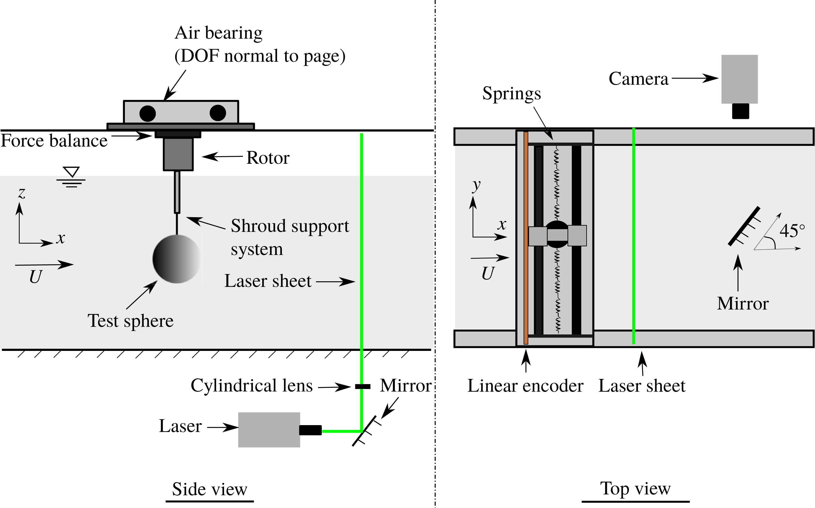
Schematic of the experimental set-up for the current study showing the side and top-down views.
2.1 Experimental details
The experiments were conducted in the recirculating free-surface water channel of the Fluids Laboratory for Aeronautical and Industrial Research (FLAIR), Monash University, Australia. The test section of the water channel is 600 mm in width, 800 mm in depth and 4000 mm in length. The free-stream velocity can be varied continuously over a range of
 $0.05\leqslant U\leqslant 0.45~\text{m}~\text{s}^{-1}$
. The free-stream turbulence level for the current experiments was less than 1 % at intermediate flow speeds.
Figure 2 shows a schematic of the current experimental set-up. The sphere was elastically mounted in the transverse direction using a low-friction air-bearing system that provides low structural damping. The structural stiffness was controlled by extension springs. More details of the hydro-elastic facility can be found in Zhao et al. (Reference Zhao, Lo Jacono, Sheridan, Hourigan and Thompson2018). A solid spherical ball of diameter
 $D=80~\text{mm}$
(accuracy within
 $\pm 0.200~\text{mm}$
) precision-machined from acrylic plastic was used in the current experiments. The sphere model had a smooth polished surface finish. It was supported with a cylindrical shroud support system. The immersed length of the total support set-up for the sphere was one diameter. A more complete description of the current experimental set-up can be found in Sareen et al. (Reference Sareen, Zhao, Lo Jacono, Sheridan, Hourigan and Thompson2018a
).
The rotary motion was driven using a miniature low-voltage micro-stepping motor (model: LV172, Parker Hannifin, US) with a resolution of 25 000 steps/revolution. The rotary oscillations were monitored using a digital optical rotary encoder (model: E5-1000, US Digital, US) with a resolution of 4000 counts/revolution. The sphere displacement was measured using a linear encoder (model: RGH24, Renishaw, UK) with a resolution of
 $1~\unicode[STIX]{x03BC}\text{m}$
. The data acquisition and the controls of the flow velocity and the sphere oscillations were automated via customised LabVIEW programs. For each data set, the signal was acquired at a sampling frequency of 100 Hz for more than 100 vibration cycles. The natural frequencies and structural damping of the system in both air and water were measured by conducting free decay tests individually in air and in quiescent water. The natural frequencies in air and water were found to be
 $f_{na}=0.208\pm 0.005$
and
 $f_{nw}=0.200\pm 0.005$
, respectively. The structural damping ratio with consideration of the added mass was determined to be
 $\unicode[STIX]{x1D701}=4.3\times 10^{-3}\pm 0.0006$
. The results in the current study are reported for a mass ratio of
 $m^{\ast }=12.116\pm 0.004$
.
To gain better insight into the flow dynamics, particle image velocimetry (PIV) measurements were employed in the cross-plane, 1.5 diameters downstream of the sphere. The flow was seeded with
 $13~\unicode[STIX]{x03BC}\text{m}$
hollow micro-spheres having a specific weight of
 $1.1~\text{g}~\text{m}^{-3}$
. A continuous laser (model: MLL-N-532-5W, CNI, China) was used to illuminate a laser plane of
 ${\sim}3~\text{mm}$
thickness aligned parallel to the
 $y$
–
 $z$
plane. A mirror was placed at
 $45^{\circ }$
angle to the free-stream direction towards the downstream side of the sphere. The mirror was placed more than 6 diameters downstream of the sphere to limit any upstream disturbance. A distance of
 ${\approx}2$
diameters is sufficient to avoid any upstream effect of the mirror in this set-up (see Venning Reference Venning2016). Imaging was performed using a high-speed camera (model: Dimax S4, PCO, AG) with a resolution of
 $2016\times 2016~\text{pixels}^{2}$
. The camera was equipped with a 105 mm Nikon lens, giving a magnification factor of
 $10.73~\text{pixel}~\text{mm}^{-1}$
for the field-of-view. Velocity fields were deduced using in-house PIV software developed originally by Fouras, Lo Jacono & Hourigan (Reference Fouras, Lo Jacono and Hourigan2008), using
 $32\times 32~\text{pixel}^{2}$
interrogation windows in a grid layout with 50 % window overlap. All the vorticity fields shown in the current study were phase-averaged over more than 100 cycles. For each PIV measurement case, a set of 3100 image pairs were collected by sampling at 10 Hz. Each image set was sorted into 24 phase bins based on the sphere’s displacement and velocity, resulting in more than 120 image pairs for averaging at each phase. The final phase-averaged vorticity fields were smoothed slightly using an iterative Laplace filter to remove small length-scale structures and to better highlight the larger-scale structures that dominate the wake.
3 VIV response of a sphere without control
In this section, we provide a brief overview of what is already known for an elastically mounted sphere undergoing VIV. A more detailed validation study based on the VIV response of an elastically mounted sphere without imposed rotation can be found in Sareen et al. (Reference Sareen, Zhao, Lo Jacono, Sheridan, Hourigan and Thompson2018a ,Reference Sareen, Zhao, Sheridan, Hourigan and Thompson b ).
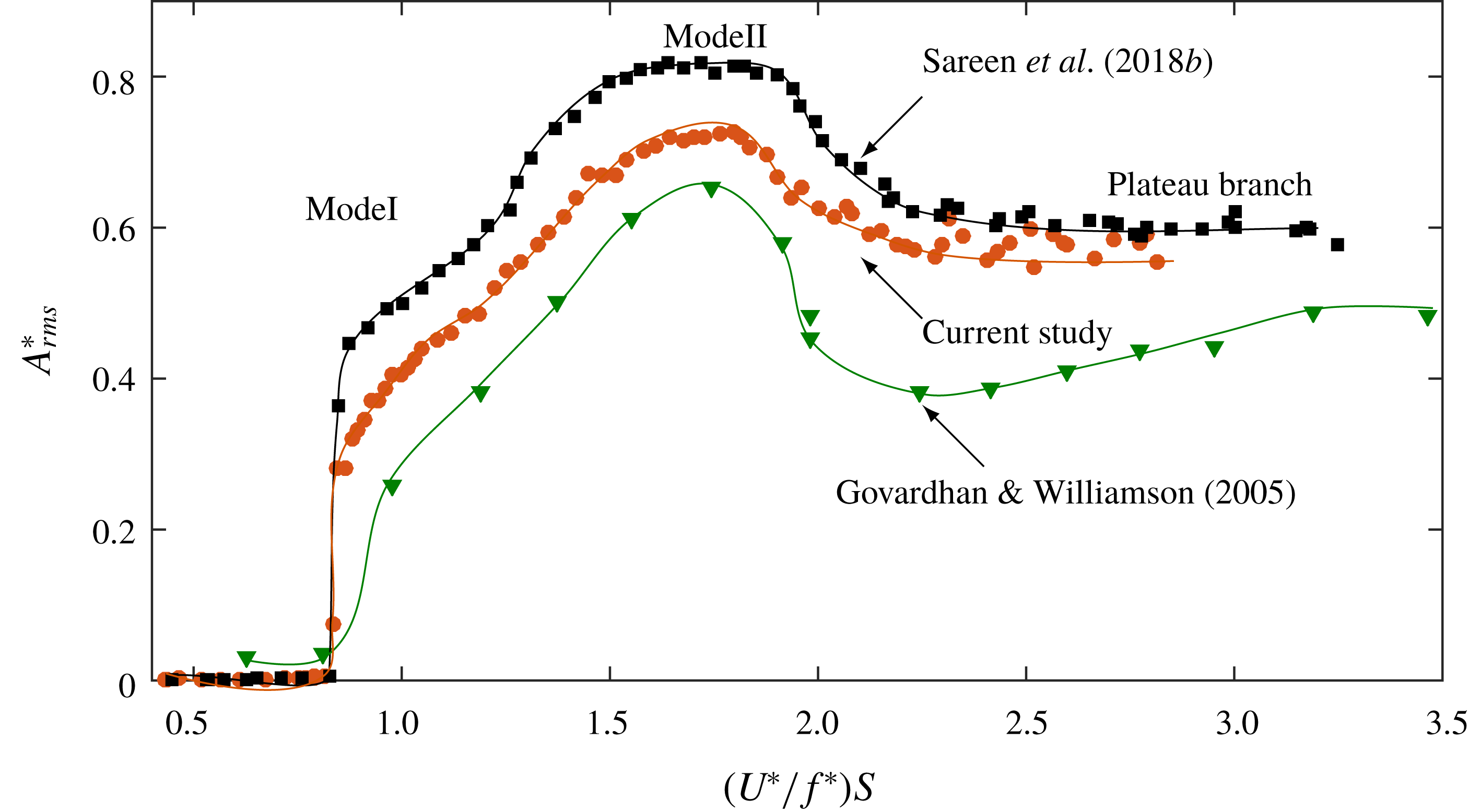
Amplitude response of an elastically mounted sphere (1-DOF) obtained in the current study (●) with a mass damping of
 $(m^{\ast }+C_{A})\unicode[STIX]{x1D701}=0.03$
compared to previous studies by Govardhan & Williamson (Reference Govardhan and Williamson2005) (▼) with a mass damping approximately 0.92 and Sareen et al. (Reference Sareen, Zhao, Sheridan, Hourigan and Thompson2018b
) (▪) with a mass damping of 0.0169.
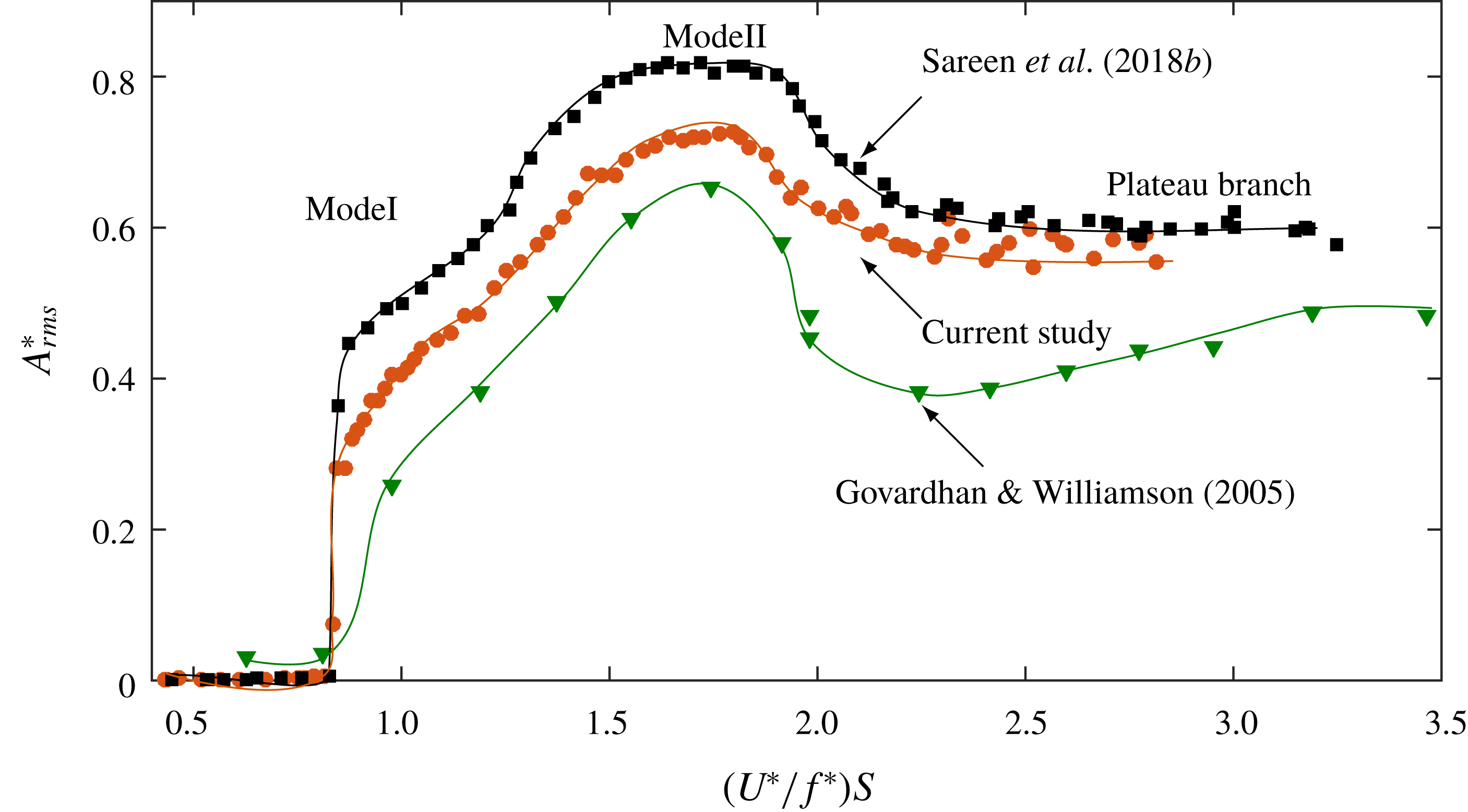
The VIV response of an elastically mounted sphere (1-DOF) without imposed rotation consists of two fundamental modes of vibration, modes I and II, in the synchronisation region followed by a ‘plateau branch’, which appears to be a precursor to mode III, seen at higher reduced velocities (Govardhan & Williamson Reference Govardhan and Williamson2005; Sareen et al.
Reference Sareen, Zhao, Lo Jacono, Sheridan, Hourigan and Thompson2018a
,Reference Sareen, Zhao, Sheridan, Hourigan and Thompson
b
). The vibrations in the plateau region are not as highly periodic as the vibrations in mode II, albeit that the frequency of oscillation stays close to the natural frequency of the system for the entire
 $U^{\ast }$
range. Although the vortex shedding remains similar in all three modes of vibration, there is a change in the timing of the vortex formation. Govardhan & Williamson (Reference Govardhan and Williamson2005) and Sareen et al. (Reference Sareen, Zhao, Lo Jacono, Sheridan, Hourigan and Thompson2018a
,Reference Sareen, Zhao, Sheridan, Hourigan and Thompson
b
) showed that the sphere vibration response transitions from mode I to mode II when the phase difference between the vortex force and the sphere displacement,
 $\unicode[STIX]{x1D719}_{vortex}$
, crosses through
 $90^{\circ }$
, corresponding to an inflection point in the amplitude response. Similarly, within mode II, the phase difference between the total transverse force and sphere displacement,
 $\unicode[STIX]{x1D719}_{total}$
, passes through
 $90^{\circ }$
, corresponding to the peak of the amplitude response. The variations of
 $\unicode[STIX]{x1D719}_{total}$
and
 $\unicode[STIX]{x1D719}_{vortex}$
for the current experimental set-up can be found in Sareen et al. (Reference Sareen, Zhao, Lo Jacono, Sheridan, Hourigan and Thompson2018a
,Reference Sareen, Zhao, Sheridan, Hourigan and Thompson
b
).
Unlike the case of a tethered sphere with 2-DOF, where the modes are separated by a desynchronised reduced velocity range (Jauvtis et al.
Reference Jauvtis, Govardhan and Williamson2001; Govardhan & Williamson Reference Govardhan and Williamson2005), the vibration amplitude for a sphere in the 1-DOF case increases gradually and continuously from mode I to mode II (
 $4.5\lesssim U^{\ast }\lesssim 15$
) leading to an almost constant amplitude in the plateau branch (
 $15\leqslant U^{\ast }<30$
). Although it is difficult to demarcate the two modes in the 1-DOF case, there are considerable changes in the phase difference between the sphere displacement and the total transverse force
 $\unicode[STIX]{x1D719}_{total}$
, and the phase difference between the sphere displacement and the vortex force,
 $\unicode[STIX]{x1D719}_{vortex}$
. The response transitions from mode I to mode II when
 $\unicode[STIX]{x1D719}_{vortex}$
crosses through
 $90^{\circ }$
, corresponding to the ‘inflection point’ in the amplitude response. Likewise, within the mode II regime,
 $\unicode[STIX]{x1D719}_{total}$
passes continuously through
 $90^{\circ }$
, corresponding to the peak of the amplitude response (Govardhan & Williamson Reference Govardhan and Williamson2005; Sareen et al.
Reference Sareen, Zhao, Lo Jacono, Sheridan, Hourigan and Thompson2018a
,Reference Sareen, Zhao, Sheridan, Hourigan and Thompson
b
). Lowering the mass-damping parameter
 $(m^{\ast }+C_{A})\unicode[STIX]{x1D701}$
leads to greater vibration amplitudes and a widened synchronisation regime, as shown in figure 3. The mass damping of the current study is
 $(m^{\ast }+C_{A})\unicode[STIX]{x1D701}=0.03$
, compared to approximately 0.92 in the study by Govardhan & Williamson (Reference Govardhan and Williamson2005) and 0.0169 in the study by Sareen et al. (Reference Sareen, Zhao, Sheridan, Hourigan and Thompson2018b
). When plotted against the scaled
 $U_{S}^{\ast }$
, defined as
 $U_{S}^{\ast }=(U^{\ast }/f^{\ast })S\equiv f_{vo}/f$
, where
 $S$
is the Strouhal number for vortex shedding (
 ${\approx}0.18$
in this case), the saturation amplitudes (peaks) line up for all the results with different mass-damping parameters, as was demonstrated by Govardhan & Williamson (Reference Govardhan and Williamson2005).
4 Effect of rotary oscillations on the vibration response
4.1 Effect of the forcing frequency ratio
In this section, the effect of forcing frequency ratio,
 $f_{R}$
, on the sphere VIV response is discussed. The response is studied for a wide range of frequency ratios varying from 0 to 5 in small increments at several fixed velocity ratios; however, only a few of the representative cases are discussed in detail here. The results are presented for three
 $U^{\ast }$
values of
 $U^{\ast }=6$
, 10 and 15, corresponding to modes I, II and mode III, respectively, of the sphere VIV response.
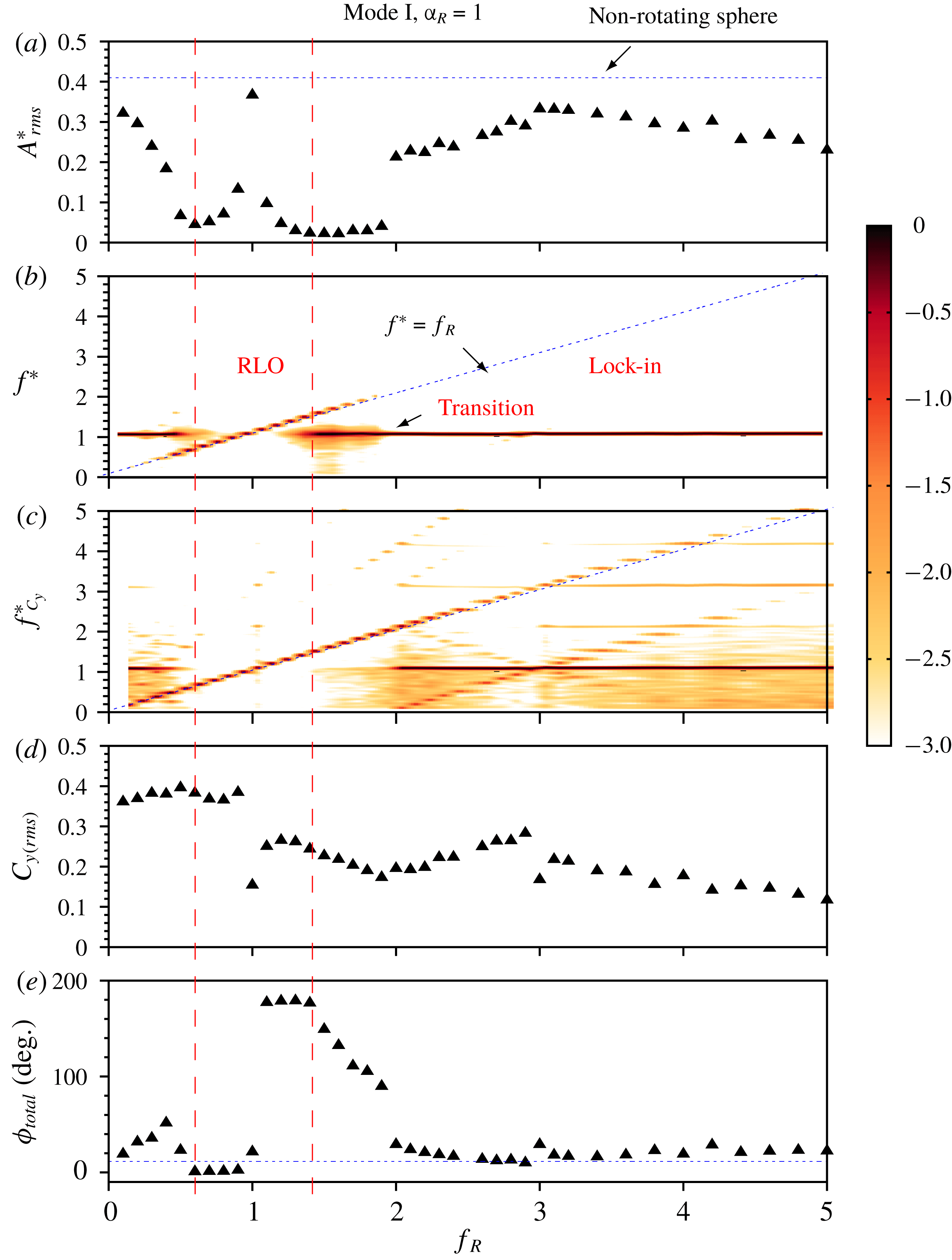
The response of an elastically mounted sphere under imposed rotary oscillation is presented as a function of forcing frequency ratio,
 $f_{R}$
, at a fixed velocity ratio of
 $\unicode[STIX]{x1D6FC}_{R}=1$
for the mode 1 response (
 $U^{\ast }=6$
). (a) The variation of r.m.s. of the oscillation amplitude (
 $A_{rms}^{\ast }$
). The dotted line represents the amplitude of a sphere with no imposed rotation. (b,c) Power spectral density (PSD) contour plots of the sphere displacement signal and the total transverse force (coefficient), respectively. The dotted line represents where the normalised frequency response,
 $f^{\ast }$
, equals the forcing frequency ratio
 $f_{R}$
. (d) The variation of the r.m.s. force coefficient of the total transverse lift
 $C_{y\,(rms)}$
. (e) The variation of the total phase difference,
 $\unicode[STIX]{x1D719}_{total}$
. The horizontal dotted line shows
 $\unicode[STIX]{x1D719}_{total}$
for a non-rotating sphere. The dashed vertical lines indicate the approximate lock-on boundaries. Note that the colour bar applies to the frequency plot, indicating the normalised spectral power on a
 $\log _{10}$
scale.
Time traces of the sphere displacement in mode I for different frequency ratios of (a)
 $f_{R}=0.3$
, (b)
 $f_{R}=0.5$
, (c)
 $f_{R}=1$
, (d)
 $f_{R}=1.9$
and (e)
 $f_{R}=4$
. The velocity ratio is fixed at
 $\unicode[STIX]{x1D6FC}_{R}=1$
.

4.1.1 Mode I
Figure 4(a) shows the variation of the r.m.s. of the amplitude of the sphere oscillations,
 $A_{rms}^{\ast }$
, with
 $f_{R}$
. Figures 4(b) and 4(c) present the frequency power spectral density (PSD) contours of the sphere displacement and the total transverse force, respectively. Figures 4(d) and (e) show the variation of the coefficient of the total transverse force,
 $C_{y\,(rms)}$
, and the total phase difference,
 $\unicode[STIX]{x1D719}_{total}$
, respectively.
As evident in figure 4(a), when
 $f_{R}$
is gradually increased from 0 to
 ${\sim}0.5$
,
 $A_{rms}^{\ast }$
progressively decreases in magnitude. The vibrations remain locked to the natural frequency of the system, i.e.
 $f^{\ast }=1$
, as shown in figure 4(b). Although the frequency response shows a clear dominant frequency at
 $f^{\ast }=1$
, the displacement is modulated in the presence of the forcing, as is clear from the time trace of the sphere displacement shown in figure 5(a). As is also evident from figure 4(c), unlike the frequency contour plot of the sphere displacement, the PSD of the total transverse force does not show a single frequency in this region. Previous studies on rotationally oscillating cylinders have also noted highly modulated states in the non-lock-on regions (Choi et al.
Reference Choi, Choi and Kang2002).
When
 $f_{R}$
is further increased to higher values beyond 0.5, the vibrations start to lock on to
 $f_{R}$
instead of
 $f_{nw}$
, as is clearly discernible in figure 4(b). Figure 4(c) shows that the total lift force also locks on to
 $f_{R}$
. This marks the start of the rotary lock-on (RLO) region that extends from
 $0.5\lesssim f_{R}\lesssim 1.5$
(bounded by dashed vertical lines). In the RLO region, the vibrations and the total transverse force are locked to the forcing frequency instead of the natural frequency, which prohibits the fluid–structure energy transfer. The vibrations are highly suppressed in this range except the case when all the characteristic frequencies of the system are equal, i.e.
 $f_{R}=f^{\ast }=f_{nw}$
; here, the vibration amplitude is close to that of a sphere without imposed rotation, and the displacement signal is highly periodic as shown in figure 5(c). In the RLO region,
 $C_{y\,(rms)}$
drops to lower values with a sudden dip for the
 $f_{R}=f^{\ast }=f_{nw}$
case (shown in figure 4
d). Also, figure 4(e) shows that there is a sudden jump in the total phase difference,
 $\unicode[STIX]{x1D719}_{total}$
, from almost
 $0^{\circ }$
(in phase) to
 $180^{\circ }$
(out of phase). Such a sudden jump in
 $\unicode[STIX]{x1D719}_{total}$
is associated with the change in the timing of vortex formation, as will be shown later in § 5 through wake measurements. Such a region of rotary lock-on, where the sphere displacement locks on to the forcing frequency, has also been observed recently for an elastically mounted cylinder under imposed rotary oscillation in the experimental study by Wong et al. (Reference Wong, Zhao, Lo Jacono, Thompson and Sheridan2018). They also observed a sudden jump in
 $\unicode[STIX]{x1D719}_{total}$
from
 $0^{\circ }$
to
 $180^{\circ }$
for a cylinder in the rotary lock-on region.
One can also note a transition region near the lock-on boundaries in figure 4(b). This region has a richness in frequency content and relatively broadened spectral densities that appear to be caused by competing
 $f_{nw}$
and
 $f_{r}$
. This is clearer for higher
 $U^{\ast }$
responses shown later in this section. The time traces of the displacement signal near the boundaries (shown in figures 5
b and 5
d) indicate a quasi-periodic state. Baek & Sung (Reference Baek and Sung2000) previously reported quasi-periodic states near the lock-on boundaries for a cylinder. When
 $f_{R}$
is further increased to higher values,
 $f_{R}>2$
, the vibrations again start to lock in to the natural frequency of the system instead of the forcing frequency. For
 $2<f_{R}\leqslant 5$
, the vibration amplitudes and
 $\unicode[STIX]{x1D719}_{total}$
recover and become close to their initial values without imposed rotation (shown in a and d). The time trace of the sphere displacement (figure 5
e) shows a highly periodic response in this range.
Figure 6 shows the response characteristics, similar to those shown previously, but for a relatively higher velocity ratio of
 $\unicode[STIX]{x1D6FC}_{R}=1.5$
in mode I. One can clearly see the difference that the transition region (or the non-lock-on region, where the flow is neither locked in nor locked on), where a wide spectrum of frequencies is observed, now extends for a wider range of
 $f_{R}$
values between
 $1.5\lesssim f_{R}\lesssim 3$
. Also, the lock-in region is observed for a narrow range of high
 $f_{R}$
values in the range
 $3<f_{R}<5$
. The vibration amplitude in the lock-in region does not recover to the values close to the non-rotating case but rather remains
 ${<}0.2D$
. So, as the velocity ratio is increased to
 $\unicode[STIX]{x1D6FC}_{R}=1.5$
, the transition region becomes wider, and lock-in occurs for a narrow range of
 $f_{R}$
values. For even higher velocity ratio of
 $\unicode[STIX]{x1D6FC}_{R}=2$
(not discussed here), the lock-in region disappears, and the transition range extends until the maximum
 $f_{R}$
tested in the current study.
The response of an elastically mounted sphere under imposed rotary oscillation is presented as a function of forcing frequency ratio,
 $f_{R}$
, at the fixed velocity ratio of
 $\unicode[STIX]{x1D6FC}_{R}=1.5$
in the mode I region (
 $U^{\ast }=6$
). Refer to figure 4 for further details.

The response quantities of an elastically mounted sphere with imposed rotary oscillations is presented as a function of forcing frequency ratio,
 $f_{R}$
, at a fixed velocity ratio of
 $\unicode[STIX]{x1D6FC}_{R}=0.5$
in mode II (
 $U^{\ast }=10$
). Refer to figure 4 for further details.

4.1.2 Mode II
Figure 7 shows the response quantities for
 $U^{\ast }=10$
, (in the heart of mode II) at a fixed velocity ratio of
 $\unicode[STIX]{x1D6FC}_{R}=0.5$
. One can note here that unlike mode I, the vibration amplitudes do not drop at all before entering the RLO region. However, as the sphere response enters the RLO region, the response characteristics are similar to mode I, with a sudden jump in
 $A_{rms}^{\ast }$
for
 $f_{R}=1$
and a corresponding drop in
 $C_{y\,(rms)}$
and
 $\unicode[STIX]{x1D719}_{total}$
. Immediately past
 $f_{R}=1$
, the vibrations become out of phase with the total transverse force, and the vibration amplitudes drop to highly reduced values. A transition region with a wide spectrum of frequencies and highly modulated vibration amplitudes (see figure 8
b) is also evident in the frequency contour plot as the response exits the RLO region. For
 $2\lesssim f_{R}\lesssim 3$
, the vibrations lock back to
 $f_{nw}$
and the vibration amplitudes start to recover. The dominant frequency of the transverse force, however, remains the forcing frequency (see figure 7
c). As the response approaches the vicinity of
 $f_{R}=3$
, the vibrations lock on to the third subharmonic of the forcing frequency,
 $f^{\ast }=f_{R}/3$
, although the effect is localised to a small
 $f_{R}$
range. Figure 7(c) shows that the transverse force locks on simultaneously to the third harmonic as well. This is termed ‘tertiary lock-on’ (TLO). Such a region of tertiary lock-on has also been observed previously for a cylinder allowing 1-DOF transverse movement under imposed rotary oscillation (Wong et al.
Reference Wong, Zhao, Lo Jacono, Thompson and Sheridan2018), and also for a rigidly mounted cylinder (Choi et al.
Reference Choi, Choi and Kang2002; Thiria et al.
Reference Thiria, Goujon-Durand and Wesfreid2006). The TLO region is also characterised by a sudden jump in
 $\unicode[STIX]{x1D719}_{total}$
and
 $C_{y\,(rms)}$
, as evident from figures 7(e) and (d), respectively. The time trace of the sphere displacement reveals a highly periodic response in the TLO region (see figure 8
c). As the sphere exits the TLO region, the dominant frequency again becomes
 $f_{nw}$
; however, unlike standard lock-in, there is no clean single frequency response. The vibrations exhibit amplitude modulation, as evident from figure 8(d). The vibration amplitude drops to lower values,
 ${\sim}0.2$
, and remains almost constant until
 $f_{R}=5$
.
Time traces of the sphere displacement in mode II for different frequency ratios of (a)
 $f_{R}=1.1$
, (b)
 $f_{R}=2$
, (c)
 $f_{R}=3$
and (d)
 $f_{R}=4.8$
. The velocity ratio is fixed at
 $\unicode[STIX]{x1D6FC}_{R}=0.5$
.

It is interesting to see how the response changes as the velocity ratio is increased to
 $\unicode[STIX]{x1D6FC}_{R}=1$
. Figure 9 shows the observed response for a higher velocity ratio of
 $\unicode[STIX]{x1D6FC}_{R}=1$
in mode II. The lock-in and the tertiary lock-on regions are absent for
 $\unicode[STIX]{x1D6FC}_{R}=1$
, unlike the
 $\unicode[STIX]{x1D6FC}_{R}=0.5$
case. Again, the vibration amplitude for the
 $f_{R}=f^{\ast }=f_{nw}$
case in the mode II region is even higher than the non-rotating case (shown as a dashed line in a). An interesting point to note here is that for
 $f_{R}>2$
, although
 $\unicode[STIX]{x1D719}_{total}$
recovers to its initial non-rotating values, the vibration amplitude does not recover to its initial value as observed in mode I. Near the lock-on boundaries, a rich frequency content is observed, however; it extends until
 $f_{R}=3$
. For
 $f_{R}>3$
, the frequency no longer follows the
 $f_{R}$
line and the vibration is highly reduced. In this case, the vibration is neither locked in (as characterised by a single frequency response at
 $f^{\ast }=1$
) nor locked on (as characterised by a single frequency response at
 $f^{\ast }=f_{R}$
). Interestingly, the dominant frequency of the lift force remains
 $f_{R}$
for
 $f_{R}>3$
. Overall, the characteristics of the RLO region remain the same with a sudden jump in
 $\unicode[STIX]{x1D719}_{total}$
from
 $0^{\circ }$
to
 $180^{\circ }$
, and a drop in
 $C_{y\,(rms)}$
correlated with the jump in
 $A_{rms}^{\ast }$
.
The response of an elastically mounted sphere with imposed rotary oscillations is presented as a function of forcing frequency ratio,
 $f_{R}$
, at a fixed velocity ratio of
 $\unicode[STIX]{x1D6FC}_{R}=1$
in mode II (
 $U^{\ast }=10$
). Refer to figure 4 for further details.

4.1.3 Mode III
Figure 10 shows the response curves at even higher
 $U^{\ast }$
values towards the mode III region. As evident from the figure, the width of rotary lock-on region is decreased in mode III, extending only between
 $0.8<f_{R}<1.4$
. Another interesting point to note is that for the
 $f_{R}=f^{\ast }=f_{nw}$
case, the vibration amplitude reaches a value of more than one sphere diameter, which is
 ${\sim}66\,\%$
higher than for the non-rotating case. The imposed rotation is very effective in mode III in suppressing vibration for the entire range of
 $f_{R}$
tested in the current study (except of course the
 $f_{R}=f_{nw}$
resonant case). The response characteristics in mode III are quite similar to mode II (the
 $\unicode[STIX]{x1D6FC}_{R}=1$
case), where the vibrations do not recover to higher values after exiting the rotary lock-on region, and a broad frequency spectrum is observed for higher
 $f_{R}$
values. However, in mode III, the vibration frequency and the lift frequency follows the
 $f^{\ast }=f_{R}$
line for the entire range of
 $f_{R}$
tested, unlike in the case of mode II. It appears that the transition region extends until
 $f_{R}=5$
in this case. Interestingly, a clean single frequency response is observed for the lift force for
 $2\lesssim f_{R}\lesssim 4$
, as seen in figure 10(c).
The response of an elastically mounted sphere with imposed rotary oscillations is presented as a function of forcing frequency ratio,
 $f_{R}$
, at a fixed velocity ratio of
 $\unicode[STIX]{x1D6FC}_{R}=1$
in mode III (
 $U^{\ast }=15$
). Refer to figure 4 for further details.

The response quantities of an elastically mounted sphere with imposed rotary oscillations is presented as a function of velocity ratio,
 $\unicode[STIX]{x1D6FC}_{R}$
, at fixed frequency ratios of
 $f_{R}=1.2$
(a,c,e) and
 $f_{R}=3$
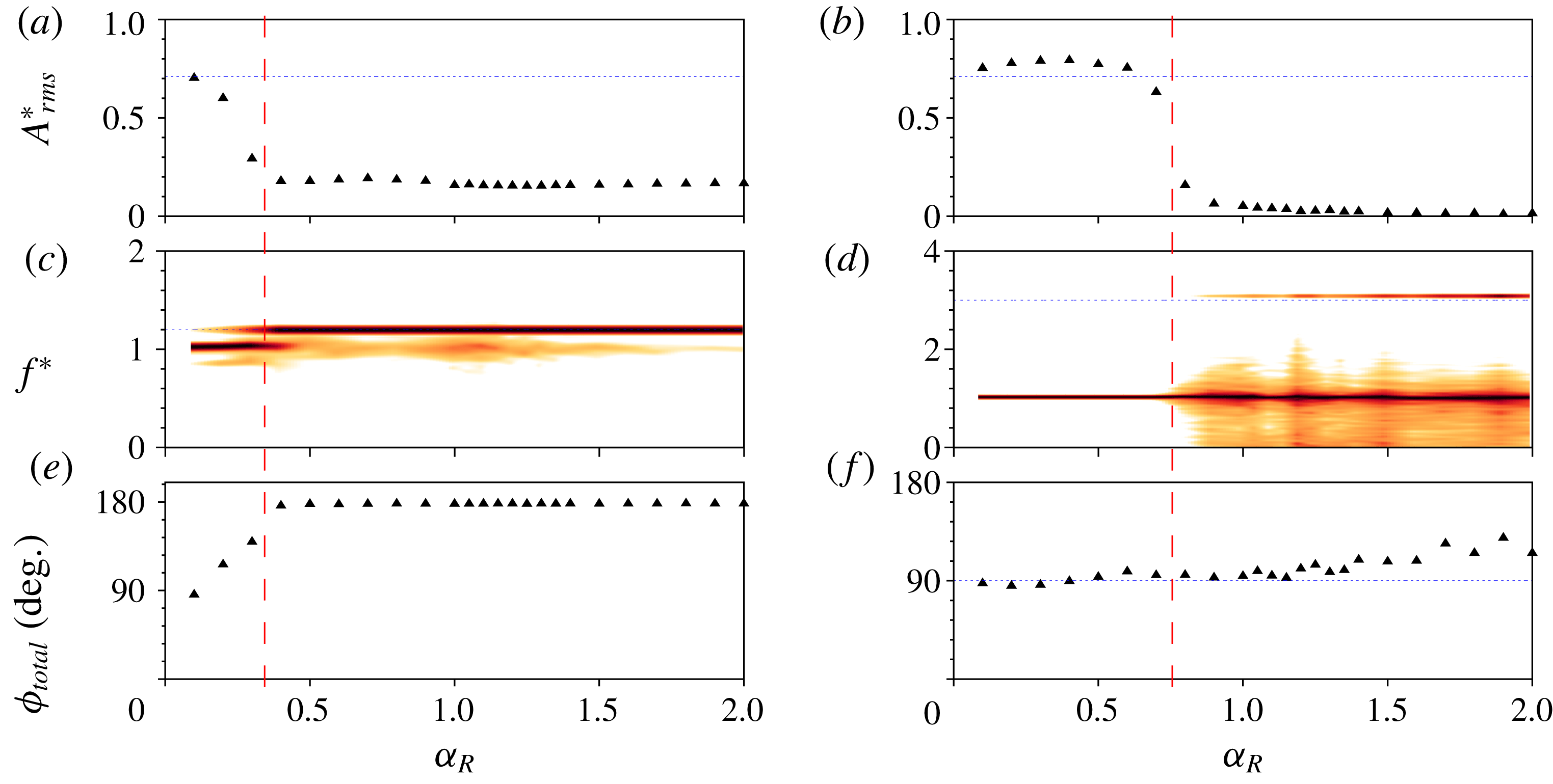
(b,d,f) in mode II. The dashed red line demarcates the two regions obtained as the velocity ratio is varied in the above cases. The vibrations are greatly suppressed beyond the dashed line for both the frequency ratios shown above.

4.2 Effect of velocity ratio
In this section, the effect of another important forcing parameter on the sphere vibration response, the velocity ratio
 $\unicode[STIX]{x1D6FC}_{R}$
, is investigated. The velocity ratio was varied over the range
 $0\leqslant \unicode[STIX]{x1D6FC}_{R}\leqslant 2$
in small increments, keeping constant values of
 $U^{\ast }$
and
 $f_{R}$
. The response was studied for
 $U^{\ast }=10$
(heart of mode II) and frequency ratios of
 $f_{R}=1$
(resonance),
 $f_{R}=1.2$
(lock-on) and
 $f_{R}=3$
(non-lock-on).
Figure 11(a) shows the response as a function of
 $\unicode[STIX]{x1D6FC}_{R}$
at a constant value of
 $f_{R}=1.2$
in mode II. It can be seen that when the velocity ratio is increased gradually to
 $\unicode[STIX]{x1D6FC}_{R}=0.5$
, there is a progressive decrease in
 $A_{rms}^{\ast }$
. The dominant frequency remains as
 $f_{nw}$
(see figure 11
c). However, when
 $\unicode[STIX]{x1D6FC}_{R}$
is increased beyond 0.5, the oscillation frequency locks on to the forcing frequency (
 $f^{\ast }=1.2$
), as shown in figure 11(c), and the displacement becomes out of phase with the total transverse force, as shown in figure 11(e). The vibrations are highly suppressed for
 $\unicode[STIX]{x1D6FC}_{R}\geqslant 0.5$
with
 ${\sim}77.7\,\%$
reduction in the vibration amplitude compared to the case of a sphere without imposed rotation. This demonstrates that values of
 $\unicode[STIX]{x1D6FC}_{R}\geqslant 0.5$
are desirable for effective suppression of VIV in mode II, at least for
 $f_{R}=1.2$
. An obvious question is that when
 $f_{R}$
is outside the lock-on range, what velocity ratios are favourable for reducing the amplitude of oscillations?
To answer this question, another frequency ratio was chosen in the non-lock-on range and the response was investigated. Figure 11(b,d,f) shows the response quantities for
 $f_{R}=3.0$
in mode II. Initially, when
 $\unicode[STIX]{x1D6FC}_{R}$
is increased, there are no significant changes in the vibration amplitude compared to the case of the sphere without any imposed forcing. The oscillations are locked to the natural frequency of the system, as shown in figure 11(d). However, there is a sharp reduction in
 $A_{rms}^{\ast }$
beyond
 $\unicode[STIX]{x1D6FC}_{R}\gtrsim 0.7$
. For higher
 $\unicode[STIX]{x1D6FC}_{R}$
values, the vibrations are suppressed completely. In the frequency spectrum plot figure 11(d), a wide spectrum of frequencies is evident for
 $\unicode[STIX]{x1D6FC}_{R}\geqslant 0.7$
. The forcing frequency
 $f_{R}=3$
is also present; however,
 $f_{nw}$
remains the dominant frequency. For this case, the sphere vibrations are neither locked in (single frequency response at
 $f^{\ast }=1$
) nor locked on (single frequency response at
 $f^{\ast }=f_{R}$
) and the frequency contour map is characterised by a wide spectrum of frequencies.
 $\unicode[STIX]{x1D719}_{total}$
remain close to
 $90^{\circ }$
for the entire range of
 $\unicode[STIX]{x1D6FC}_{R}$
(except the higher
 $\unicode[STIX]{x1D6FC}_{R}$
values, where small deviation can be observed). An interesting thing to note here is that suppression of vibrations can be observed for a sphere even in the non-lock-on range for high enough
 $\unicode[STIX]{x1D6FC}_{R}$
values.
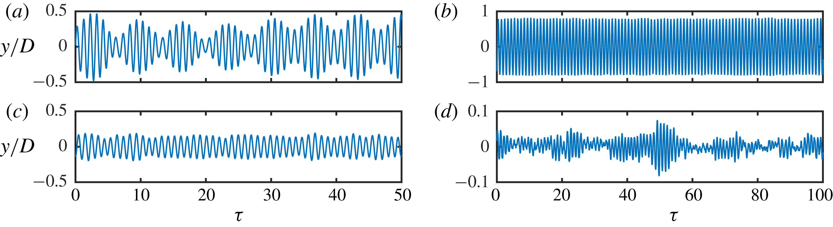
Figure 12(a,c) shows the time trace of the sphere displacement at
 $f_{R}=1.2$
for the two different velocity ratios of
 $\unicode[STIX]{x1D6FC}_{R}=0.3$
(a) and
 $\unicode[STIX]{x1D6FC}_{R}=1.3$
(c). For
 $\unicode[STIX]{x1D6FC}_{R}=0.3$
, a pulsating signal is evident with a beating frequency
 ${\sim}|f_{r}-f_{nw}|$
. For
 $\unicode[STIX]{x1D6FC}_{R}=1.3$
, on the other hand, beating is not clear and the vibrations are not very periodic. Figure 12(b,d) shows the time trace of the sphere displacement at
 $f_{R}=3$
for two different velocity ratios
 $\unicode[STIX]{x1D6FC}_{R}=0.3$
(b) and
 $\unicode[STIX]{x1D6FC}_{R}=1.3$
(d). For
 $\unicode[STIX]{x1D6FC}_{R}=0.3$
, the vibrations are highly periodic without any signs of amplitude modulation. On the contrary, at
 $\unicode[STIX]{x1D6FC}_{R}=1.3$
, where highly reduced vibrations are observed (
 $A_{rms}^{\ast }<0.08$
), the displacement signal is highly non-periodic with chaotic intermittent vibrations similar to the ones reported by Sareen et al. (Reference Sareen, Zhao, Lo Jacono, Sheridan, Hourigan and Thompson2018a
) in their experimental study on an elastically mounted sphere with imposed constant rotation.
Time traces of the sphere displacement for frequency ratios
 $f_{R}=1.2$
(a,c) and
 $f_{R}=3$
(b,d) at two different velocity ratios of
 $\unicode[STIX]{x1D6FC}_{R}=0.3$
and
 $\unicode[STIX]{x1D6FC}_{R}=1.3$
.

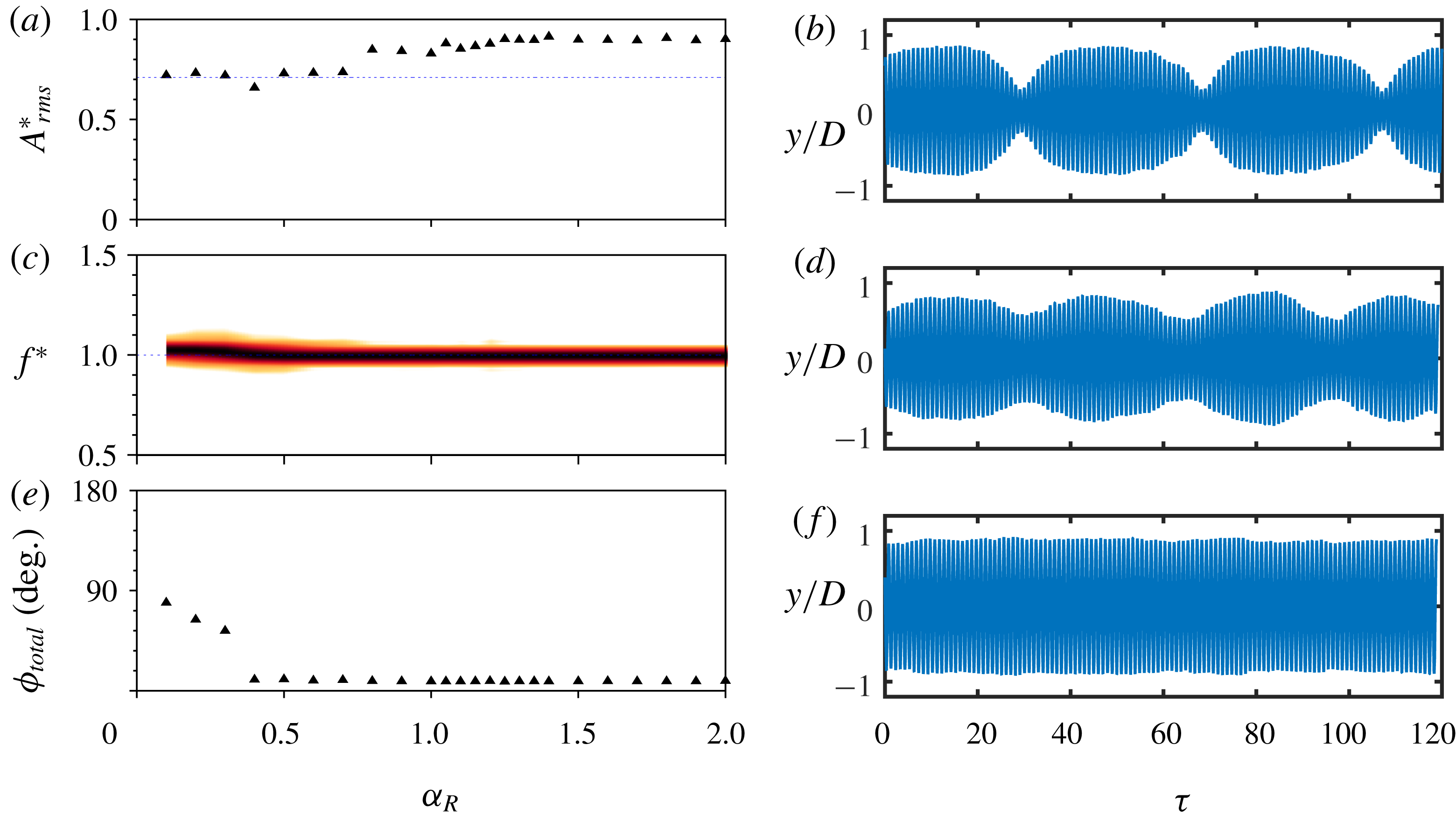
The response quantities of an elastically mounted sphere with the imposed rotary oscillations is presented as a function of velocity ratio,
 $\unicode[STIX]{x1D6FC}_{R}$
, at a fixed frequency ratio of
 $f_{R}=1$
(a,c,e) for mode II. (b,d,f) The time traces of the sphere displacement for
 $\unicode[STIX]{x1D6FC}_{R}=0.3$
(d),
 $\unicode[STIX]{x1D6FC}_{R}=0.6$
(d) and
 $\unicode[STIX]{x1D6FC}_{R}=1.2$
(f).

Another interesting case to examine is
 $f_{R}=1$
, where vibration amplitudes higher than the non-rotating case can be observed, depending on the
 $U^{\ast }$
and
 $\unicode[STIX]{x1D6FC}_{R}$
, as was shown in § 4.1. Figure 13 shows the response quantities for
 $f_{R}=1$
for varying velocity ratios in mode II. As
 $\unicode[STIX]{x1D6FC}_{R}$
increases from
 $0\leqslant \unicode[STIX]{x1D6FC}_{R}\leqslant 0.5$
,
 $\unicode[STIX]{x1D719}_{total}$
decreases almost linearly from
 $90^{\circ }$
to
 $0^{\circ }$
but the vibration amplitudes remain close to the non-rotating sphere case. In this range, the sphere displacement has modulation over a very large period of
 ${\sim}40$
cycles, as is clear from the time trace of the sphere displacement shown in figure 13(b). The degree of modulation decreases for
 $\unicode[STIX]{x1D6FC}_{R}=0.6$
(see figure 13(d)). For
 $0.5<\unicode[STIX]{x1D6FC}_{R}\leqslant 2$
, the vibration amplitudes increase by
 ${\sim}94\,\%$
compared to the non-rotating sphere case. In this range, the displacement is always in phase with the total transverse force acting on the sphere, and the vibrations become highly periodic without any signs of amplitude modulation (see figure 13(f)).
To summarise the discussions so far on the effect of the two main forcing parameters on the vibration response of a sphere, all the results are synthesised and presented as contour plots in Figure 14. Figure 14(a–c) shows the amplitude response (
 $A_{rms}^{\ast }$
) contours over the
 $f_{R}-\unicode[STIX]{x1D6FC}_{R}$
parameter space for all three modes of sphere vibrations. The contour plots show there are two observed lock-on regions: rotary lock-on (RLO) and tertiary lock-on (TLO). These regimes are determined by examining the body vibration frequency response as a function of
 $f_{R}$
for each fixed
 $\unicode[STIX]{x1D6FC}_{R}$
. Such regions have also been recently identified for an elastically mounted cylinder by Wong et al. (Reference Wong, Zhao, Lo Jacono, Thompson and Sheridan2018). Evidently, these lock-on regions are a function of all three forcing parameters:
 $f_{R}$
,
 $\unicode[STIX]{x1D6FC}_{R}$
and
 $U^{\ast }$
. For all three sphere vibration modes, the RLO region exists over a narrow window in the vicinity of
 $f_{R}=1$
. For
 $\unicode[STIX]{x1D6FC}_{R}<1$
, the RLO region occurs in a narrow band around
 $f_{R}=1$
but becomes considerably wider for higher velocity ratios, resulting in an inverted pear-shaped region. A tertiary lock-on region (TLO) was also observed in mode II in the vicinity of
 $f_{R}=3$
for very low velocity ratios of
 $\unicode[STIX]{x1D6FC}_{R}\leqslant 0.5$
. The RLO region remains fairly similar in mode I and mode II. However, for mode III, the RLO region becomes narrower for
 $\unicode[STIX]{x1D6FC}_{R}\leqslant 1$
and considerably wider for higher velocity ratios of
 $\unicode[STIX]{x1D6FC}_{R}>1.5$
. As evident from the contour plots, the reduced velocity can also influence the lock-in and TLO regions. The lock-in region becomes significantly smaller for mode II (
 $U^{\ast }=10$
) compared to mode I (
 $U^{\ast }=6$
), and vanishes completely for mode III (
 $U^{\ast }=15$
). TLO, however, was only observed for
 $f_{R}=3$
at very low velocity ratios (
 $\unicode[STIX]{x1D6FC}_{R}\leqslant 0.5$
) in mode I and mode III.
In general, mode I was found to be quite robust, requiring high velocity ratios for the suppression of vibrations. The control was highly effective in mode III, with a highly reduced response obtained over the entire parameter space studied (except for the
 $f_{R}=f_{nw}$
case). For the
 $f_{R}=f_{nw}$
case, the sphere exhibited an ‘enhanced resonance’, where vibrations increased to much higher values compared to the non-rotating case. Overall, higher velocity ratios of
 $\unicode[STIX]{x1D6FC}_{R}\geqslant 1$
were effective in suppressing the vibrations. Suppression of vibration was observed even in the non-lock-on region at high
 $f_{R}$
and
 $\unicode[STIX]{x1D6FC}_{R}$
values.
Plots showing the contours of
 $A_{rms}^{\ast }$
as a function of
 $\unicode[STIX]{x1D6FC}_{R}$
and
 $f_{R}$
in mode I (a), mode II (b) and mode III (c). Different regions highlighted with dashed lines.

4.3 Effect of reduced velocity
In this section, the effect of another important flow parameter, the reduced velocity,
 $U^{\ast }$
, is discussed. In order to systematically investigate the effect of
 $U^{\ast }$
, both the other forcing parameters (
 $\unicode[STIX]{x1D6FC}_{R}$
and
 $f_{R}$
) were kept constant and
 $U^{\ast }$
was varied in small increments from 0 to 20. The results are presented for
 $\unicode[STIX]{x1D6FC}_{R}=1$
at several representative
 $f_{R}$
values.
The response of an elastically mounted sphere with imposed rotary oscillations is presented as a function of reduced velocity for a fixed frequency ratio of
 $f_{R}=0.3$
(a) and
 $f_{R}=0.9$
(b) at
 $\unicode[STIX]{x1D6FC}_{R}=1$
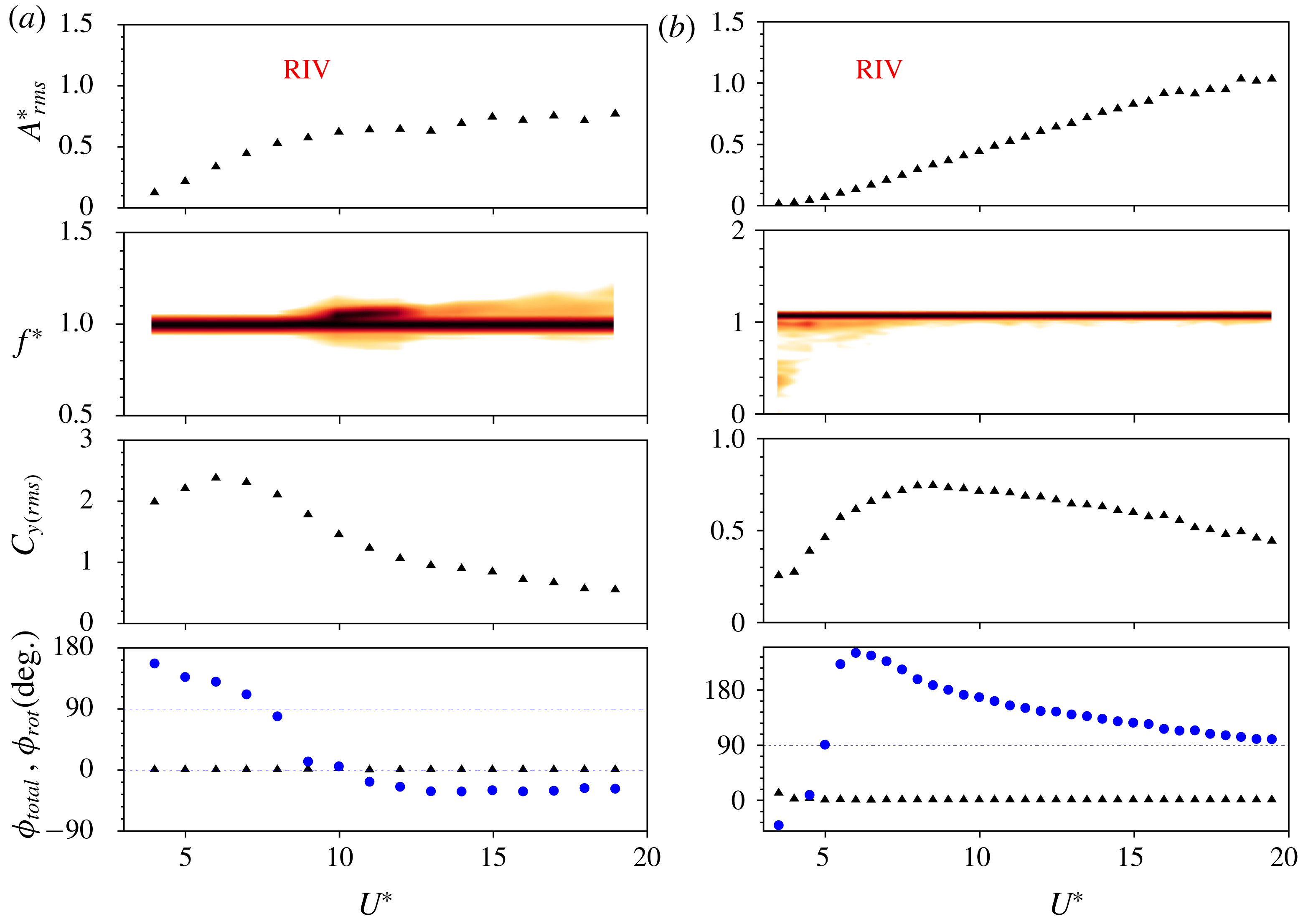
. See figure 4 for a detailed description of the figures. The blue-filled circular symbols in the phase plots represent the phase difference between the rotary oscillations and the displacement. The ‘Lock-in
 $+$
RIV’ region highlighted for
 $f_{R}=0.9$
indicates the
 $U^{\ast }$
values for which the two frequencies compete with each other.

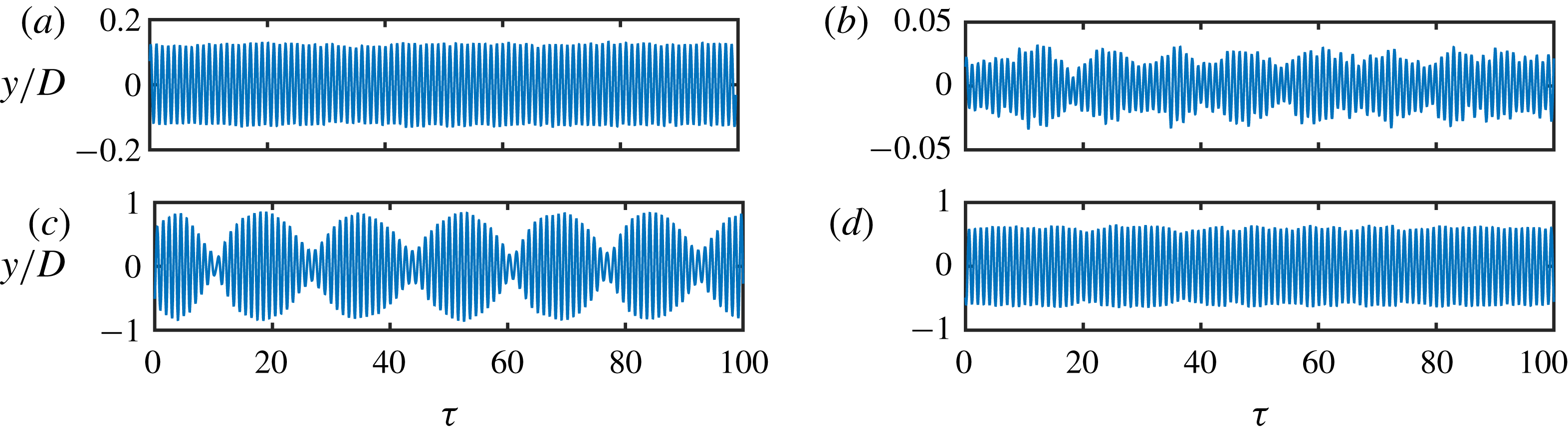
Time traces of the sphere displacement for
 $f_{R}=0.3$
(a,c) and
 $f_{R}=0.9$
(b,d) for a velocity ratio of
 $\unicode[STIX]{x1D6FC}_{R}=1$
. (a,c) Time traces for
 $U^{\ast }=8$
and 15, respectively. (b,d) Time traces for
 $U^{\ast }=6$
and
 $U^{\ast }=10$
, respectively.

Figure 15 shows the response quantities for
 $f_{R}=0.3$
(a) and
 $f_{R}=0.9$
(b) at a fixed velocity ratio of
 $\unicode[STIX]{x1D6FC}_{R}=1$
. In the plots depicting the phases, the phase difference between the imposed rotary oscillation and the sphere displacement,
 $\unicode[STIX]{x1D719}_{rot}$
, is also shown along as
 $\unicode[STIX]{x1D719}_{total}$
. It is found that
 $\unicode[STIX]{x1D719}_{rot}$
, i.e. the phase difference between the imposed rotary oscillation and the sphere displacement is an important parameter affecting the response of the sphere to the imposed rotation during lock-on conditions. Readers should note here that
 $\unicode[STIX]{x1D719}_{rot}$
is only useful in lock-on regions, where the sphere displacement is locked to the forcing frequency. As evident from panel (a), for
 $U^{\ast }$
varying from
 ${\sim}4.5$
to
 ${\sim}12$
, the vibrations are locked to the natural frequency. There is an increase in the displacement amplitude with a corresponding increase in the transverse force coefficient. The displacement is in phase with the total transverse force (or
 $\unicode[STIX]{x1D719}_{total}=0$
). The time trace of the sphere displacement shows a highly periodic response in this region (see figure 16
a). This indicates the occurrence of lock-in over this range. However, for higher values of
 $U^{\ast }>12$
,
 $\unicode[STIX]{x1D719}_{rot}$
drops to almost zero. In this region, the vibrations are locked to
 $f_{R}$
and the frequency at
 $f_{nw}$
becomes weaker in power. There is no significant increase in the amplitude response up to
 $U^{\ast }=20$
. This region cannot be termed lock-in. The time trace shows amplitude and frequency modulation in this range (see figure 16
c). In this region, the two frequencies compete with each other; such a region is termed the ‘lock-in
 $+$
RIV’ region in the text.
For
 $f_{R}=0.9$
, the response clearly has two regions with different characteristic behaviours. For
 $0\leqslant U^{\ast }\lesssim 8$
, the vibrations are locked to
 $f_{R}$
instead of
 $f_{nw}$
, and there is a linear decrease in
 $\unicode[STIX]{x1D719}_{rot}$
from
 ${\sim}130^{\circ }$
to
 $0^{\circ }$
. This is clearly not lock-in. It will be shown later in the text that such a region corresponds to the rotary-induced vibrations (RIV). Nevertheless, the time trace shows highly periodic vibrations in this range. For
 $8<U^{\ast }<14$
, on the other hand, the behaviour is similar to lock-in. The vibrations are locked to
 $f_{nw}$
, there is a jump in
 $C_{y\,(rms)}$
, and
 $\unicode[STIX]{x1D719}_{total}$
remains close to
 $0^{\circ }$
. However, the time trace of the displacement signal shows beating in this range due to
 $f_{r}$
being very close to
 $f_{nw}$
. When
 $U^{\ast }$
is increased beyond
 $U^{\ast }\geqslant 15$
, the vibrations lock to
 $f_{R}$
again. In this range, both
 $\unicode[STIX]{x1D719}_{total}$
and
 $\unicode[STIX]{x1D719}_{rot}$
approach
 $0^{\circ }$
. In this region, extending from
 $8<U^{\ast }<20$
, it can be conjectured that the two frequencies compete with each other and there is no clear lock-in or lock-on region.
Therefore, depending on the
 $U^{\ast }$
value, the vibrations may lock to
 $f_{nw}$
or
 $f_{R}$
. If vibrations lock to
 $f_{nw}$
in the synchronisation region, lock-in or resonance is observed; however, if they lock to
 $f_{R}$
, the response is reflected in
 $\unicode[STIX]{x1D719}_{rot}$
. Monotonically decreasing
 $\unicode[STIX]{x1D719}_{rot}$
values coincide with monotonically increasing
 $A_{rms}^{\ast }$
(that lead to RIV response) and constant
 $\unicode[STIX]{x1D719}_{rot}$
values coincide with constant amplitudes. This behaviour will be further clarified in later discussions.
 $\unicode[STIX]{x1D719}_{rot}$
was plotted here to highlight its correlation with the amplitude response in the lock-on regions. During lock-in, however,
 $\unicode[STIX]{x1D719}_{rot}$
does not signify anything as the displacement and rotary oscillation do not exhibit the same frequency:
 $\unicode[STIX]{x1D719}_{rot}$
is fixed at
 $90^{\circ }$
in lock-in regions.
The response of an elastically mounted sphere with imposed rotary oscillations is presented as a function of reduced velocity for a fixed frequency ratio of
 $f_{R}=1.0$
(a) and
 $f_{R}=1.1$
(b) at a value of
 $\unicode[STIX]{x1D6FC}_{R}=1$
. Refer to figure 4 for further details.

Time traces of the sphere displacement for
 $f_{R}=1$
(a,c) and
 $f_{R}=1.1$
(b,d) for reduced velocities of
 $U^{\ast }=4$
and
 $U^{\ast }=12$
.

4.3.1 Rotary-induced vibrations
Figure 17 shows the response for
 $f_{R}=1$
(a) and
 $f_{R}=1.1$
(b). Overall, it is evident that neither frequency ratio exhibits the typical bell-shaped response known for a non-rotating sphere VIV over this
 $U^{\ast }$
range. Unlike the non-rotating case,
 $\unicode[STIX]{x1D719}_{total}$
remains at
 $0^{\circ }$
for the entire range of
 $U^{\ast }$
tested. Also, the vibrations are locked to the forcing frequency. Clearly, this is not a lock-in phenomenon.
For
 $f_{R}=1$
, initially the vibration amplitude increases almost linearly in the range
 $0<U^{\ast }<10$
. In this range,
 $\unicode[STIX]{x1D719}_{rot}$
is not fixed at
 ${\sim}90^{\circ }$
, as was previously found for lock-in, but decreases monotonically from
 ${\sim}170^{\circ }$
to lower values. The vibrations are highly periodic as clear from figure 18(a), and the frequency contour plot shows a clean single frequency response at
 $f^{\ast }=1$
. Interestingly, a ‘kink’ can be observed in the frequency response when
 $\unicode[STIX]{x1D719}_{rot}$
crosses zero at
 $U^{\ast }=10$
. Beyond this point in
 $U^{\ast }$
, there are large modulations in the sphere displacement signal (at a low frequency) as evident from the time trace shown in figure 18(c). Also,
 $\unicode[STIX]{x1D719}_{rot}$
and
 $A_{rms}^{\ast }$
remain almost constant.
For
 $f_{R}=1.1$
, initially the vibrations are not very periodic in the range
 $0<U^{\ast }<6$
(see figure 18
b) but as the reduced velocity is increased further (
 $U^{\ast }\geqslant 6$
), the vibrations become periodic (see figure 18
d). For
 $U^{\ast }\geqslant 6$
, the frequency plot shows a clean frequency at
 $f^{\ast }=f_{R}=1.1$
. Also,
 $\unicode[STIX]{x1D719}_{rot}$
decreases monotonically from
 ${\sim}260^{\circ }$
to
 $90^{\circ }$
, and correspondingly, the vibration amplitude increases monotonically (almost linearly) with the increase in reduced velocity for the entire range of
 $U^{\ast }$
tested in the current study.
The response characteristics of an elastically mounted sphere with imposed rotary oscillations is presented as a function of reduced velocity for a fixed frequency ratio of
 $f_{R}=3$
(a) and
 $f_{R}=4$
(b) at a
 $\unicode[STIX]{x1D6FC}_{R}$
value of
 $\unicode[STIX]{x1D6FC}_{R}=1$
. Refer to figure 4 for further details.

The vibration response observed in the above cases show some similarities to the ‘wake-induced vibration (WIV)’ reported by Assi, Bearman & Meneghini (Reference Assi, Bearman and Meneghini2010), or called ‘wake-induced galloping’ by Bokaian & Geoola (Reference Bokaian and Geoola1984) and Brika & Laneville (Reference Brika and Laneville1999) for an elastically mounted cylinder placed downstream of a fixed cylinder. The latter studies reported that for a fixed structural damping, the downstream cylinder can exhibit vortex resonance, WIV, combined vortex resonance and WIV, or separately vortex resonance and WIV depending on the cylinders’ separation. Assi et al. (Reference Assi, Bearman and Meneghini2010) suggested that wake-induced vibration (WIV) requires a frequency input such as upstream vortex shedding to occur. They also highlighted that the upstream vortices interfering with the downstream cylinder induce fluctuations in the fluid force. A favourable phase lag between the fluid force and the displacement ensures a positive energy transfer from the flow to the structure that sustains the oscillations. One may infer here that the wake of the fixed cylinder placed upstream provides an oscillating forcing to the elastically mounted cylinder placed downstream. In the current study, however, the forcing is imposed on the sphere itself in contrast to the less controlled forcing of their study. The vibrations are not generated by a wake upstream but rather by rotary oscillations imposed on the sphere. Thus, it makes sense to describe such vibrations as ‘rotary-induced vibrations (RIV)’. Similar vibrations have also been observed recently for an elastically mounted cylinder with imposed rotary oscillation by Wong et al. (Reference Wong, Zhao, Lo Jacono, Thompson and Sheridan2018). They reported vibration increasing monotonically with
 $U^{\ast }$
for
 $f_{R}=1$
and
 $\unicode[STIX]{x1D6FC}_{R}=1$
.
Nevertheless, it should be mentioned here that the vibrations observed in the current study are very different to the galloping response known for isolated non-circular bluff bodies, that is, a low frequency phenomenon observed at very high flow velocities (Blevins Reference Blevins1990; Zhao et al.
Reference Zhao, Leontini, Lo Jacono and Sheridan2014b
). In contrast, in the current study, vibrations exhibiting RIV were always locked to the forcing frequency. It was also evident that monotonic increasing amplitudes were associated with the monotonic decreasing
 $\unicode[STIX]{x1D719}_{rot}$
values (from
 ${\sim}180^{\circ }$
to lower values). It can be conjectured here based on this evidence that RIV will only occur in the
 $U^{\ast }$
range where lock-on is observed. The case of monotonically decreasing
 $\unicode[STIX]{x1D719}_{rot}$
values from
 ${\sim}180$
to lower values leads to monotonically increasing amplitude. In cases where
 $\unicode[STIX]{x1D719}_{rot}$
remains constant, there is no appreciable increase in the vibration amplitude. In § 4.1, it was shown that the lock-on range varies with
 $U^{\ast }$
, becoming narrower with increasing
 $U^{\ast }$
. This leaves a very narrow window of
 $f_{R}$
values where lock-on, and hence RIV, can be observed for the entire range of
 $U^{\ast }$
tested in the current study.
In § 4.1, the results showed suppression of vibrations for very high frequency (
 $f_{R}\geqslant 3$
) and velocity ratios (
 $\unicode[STIX]{x1D6FC}_{R}\geqslant 1$
), even in non-lock-on regions. The question arises as to whether a specific set of parameters leads to RIV or VIV, or both? To investigate this, high frequency ratios of
 $f_{R}=3$
and
 $f_{R}=4$
were also investigated. Figure 19 shows the response characteristics for
 $f_{R}=3$
(a) and
 $f_{R}=4$
(b). A wide lock-in region is evident for both the frequencies extending from
 ${\sim}4.5$
to
 ${\sim}11$
, with a corresponding jump in the
 $C_{y\,(rms)}$
. As previously,
 $\unicode[STIX]{x1D719}_{total}$
is fixed at
 $0^{\circ }$
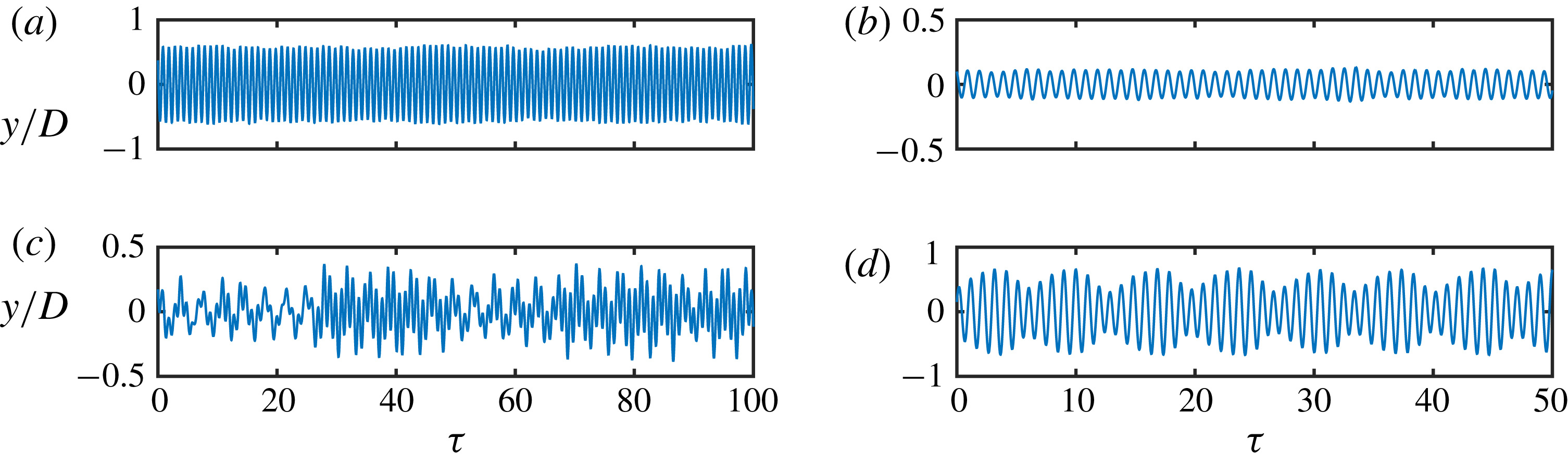
in the lock-in region, and the time trace of the displacement signal is highly periodic, as shown in figure 20 (a). When
 $U^{\ast }$
is increased beyond the lock-in region, the frequency contour plot shows a wide spectrum of frequencies. The frequency does not lock on to
 $f_{R}$
, and nor is there a clean single frequency response at
 $f^{\ast }=1$
, as observed for lock-in. Interestingly,
 $\unicode[STIX]{x1D719}_{total}$
approached
 $90^{\circ }$
in this region. The time trace of the displacement signal shows a non-periodic signal in this range (see figure 20
b).
Time traces of the sphere displacement for
 $U^{\ast }=6$
(a) and
 $U^{\ast }=18$
(b) for
 $f_{R}=3$
.

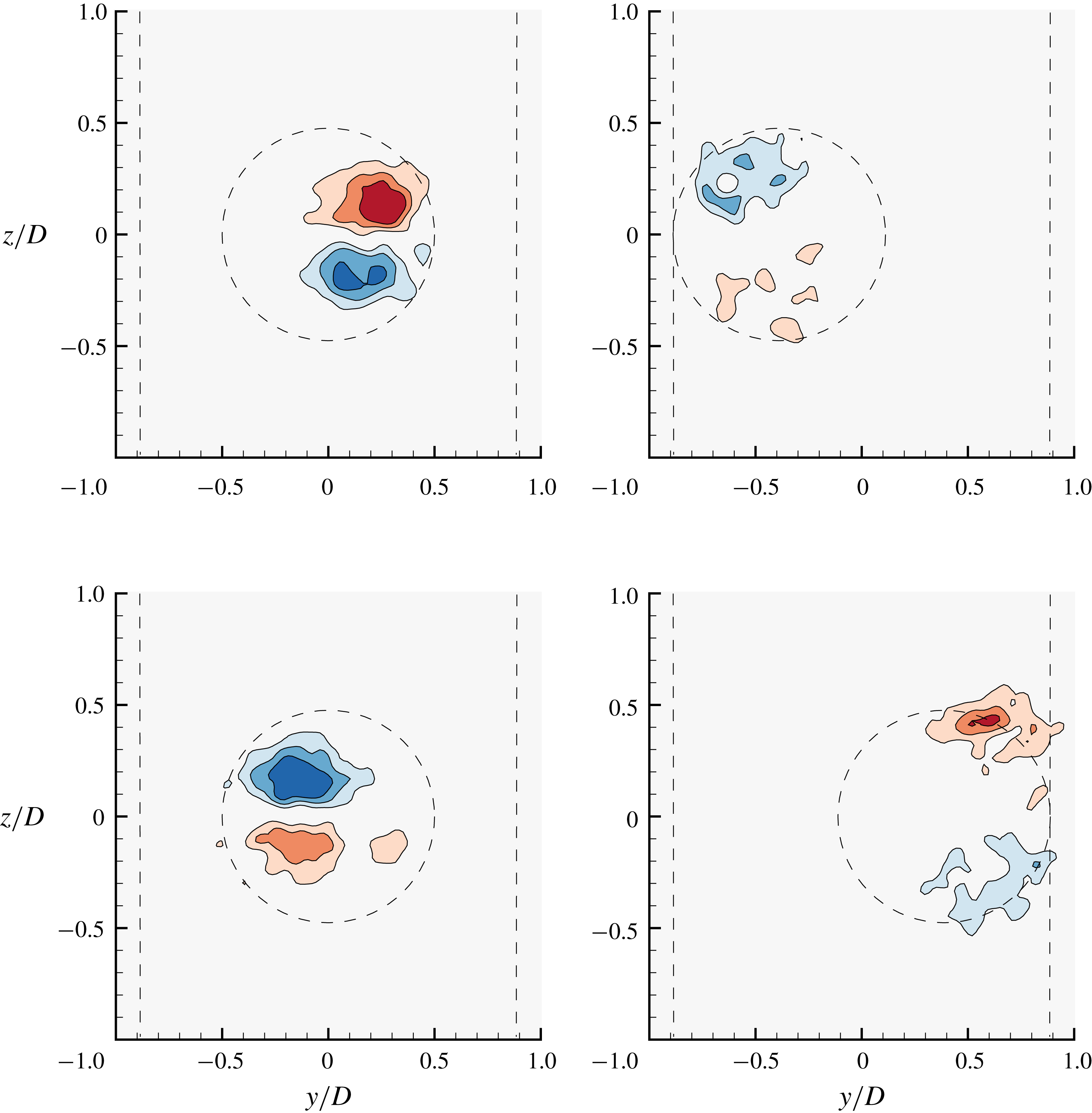
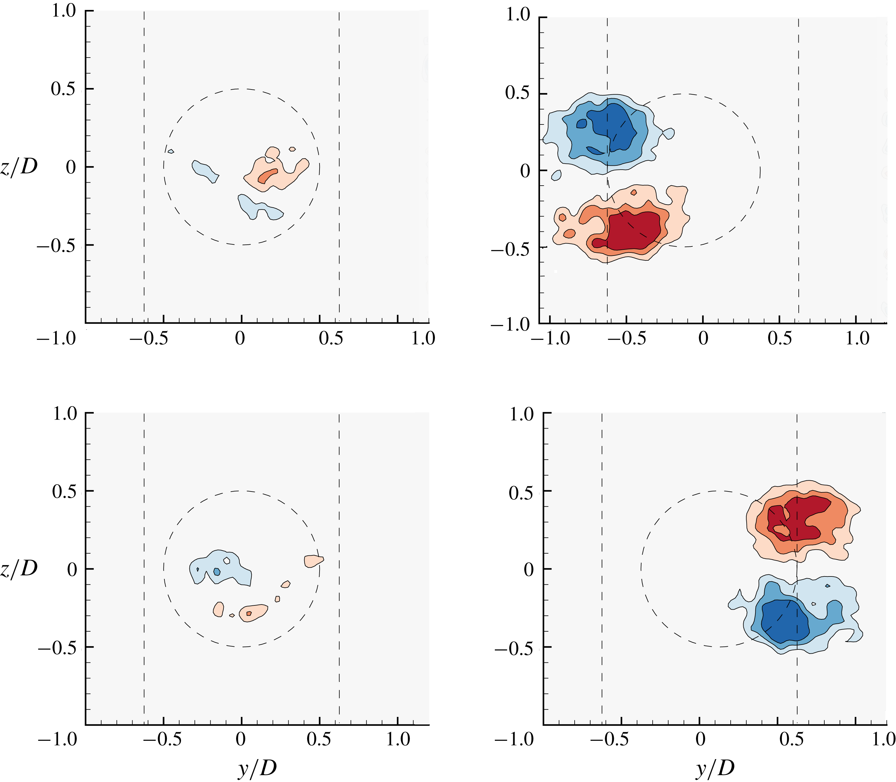
Streamwise vorticity plots showing the dominant counter-rotating vortex pair in mode I (
 $U^{\ast }=6$
) without any imposed rotation. Each of these plots are separated by a quarter period, and were measured at a distance of
 $x/D=1.5$
from the sphere. The dashed lines show the maximum displacement of the sphere and the sphere location. Blue contours show clockwise vorticity, red anti-clockwise vorticity. The normalised vorticities vary in eight steps in the range
 $\unicode[STIX]{x1D714}^{\ast }=\unicode[STIX]{x1D714}D/U$
 $\in [-3,3]$
, where
 $\unicode[STIX]{x1D714}$
is the vorticity.

5 Wake measurements
The VIV of a sphere is induced by streamwise vorticity, in contrast to its two-dimensional counterpart, the cylinder, whose dynamics is mainly induced by spanwise vorticity. PIV measurements in a plane normal to the flow can reveal important insights into the temporal evolution of the streamwise vorticity as the vortex loops pass through a cross-plane. Hence, the current study employs PIV measurements in the cross-plane at a distance of
 $1.5D$
from the sphere’s downstream surface, similar to that employed by Govardhan & Williamson (Reference Govardhan and Williamson2005) and Sareen et al. (Reference Sareen, Zhao, Sheridan, Hourigan and Thompson2018b
). Figure 21 shows the vorticity contour plots, phase-averaged over more than 100 cycles, at four different phases of the oscillation cycle, separated by a quarter period, for a sphere without any imposed rotary oscillation. The plots are shown for a reduced velocity of
 $U^{\ast }=6$
(mode I). As evident from figure 21, the streamwise vorticity consists of a dominant counter-rotating vortex pair consistent with the legs of vortex loops forming on both the sides of the sphere wake (Sakamoto & Haniu Reference Sakamoto and Haniu1990, Govardhan & Williamson Reference Govardhan and Williamson2005 and Sareen et al.
Reference Sareen, Zhao, Sheridan, Hourigan and Thompson2018b
). As the sphere traverses from one side to the other, the vorticity changes sign, corresponding to hairpin loops being shed downstream into the wake from opposite sides.
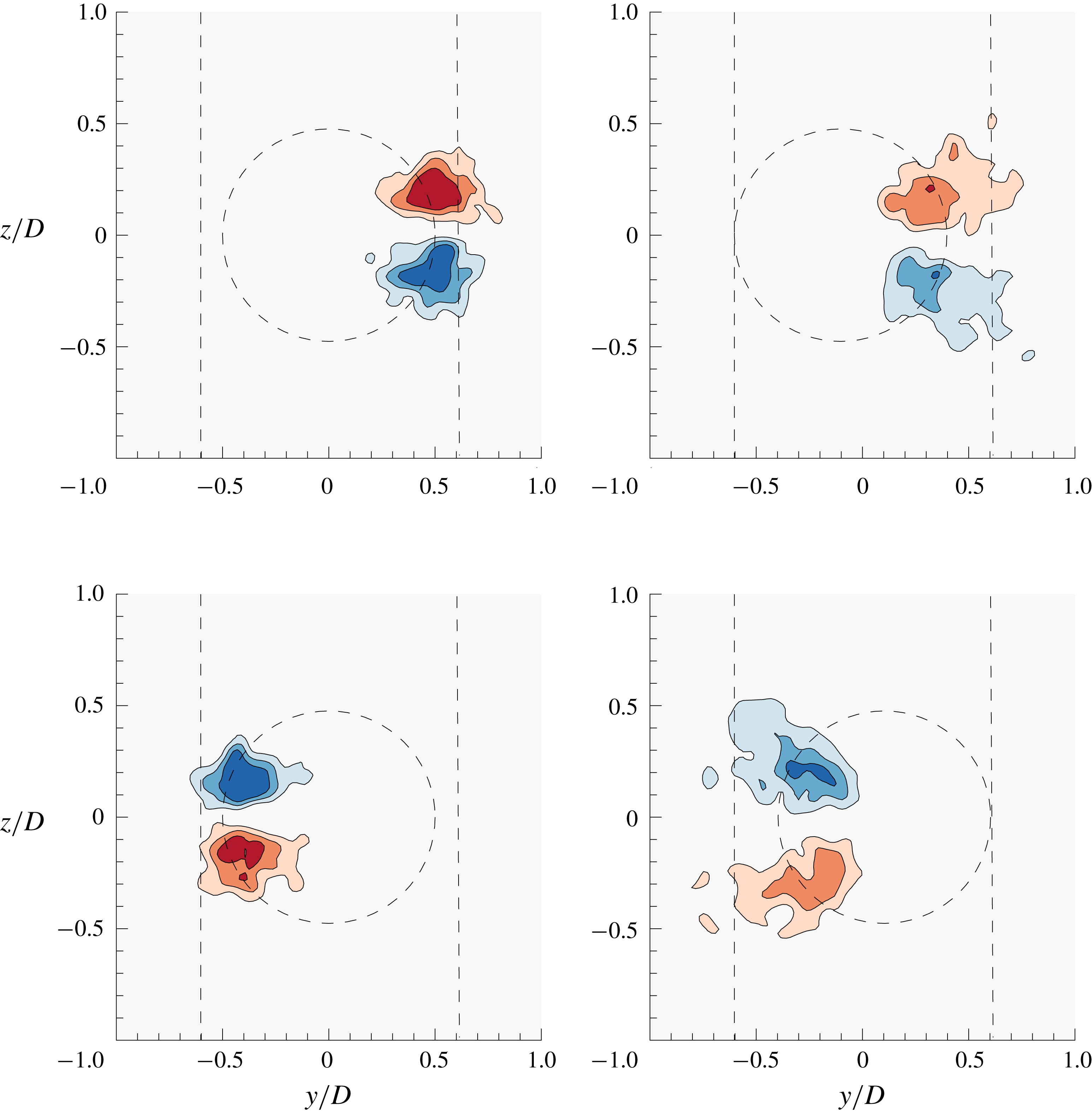
Streamwise vorticity plots showing the dominant counter-rotating vortex pair in mode I (
 $U^{\ast }=6$
) for the frequency ratio of
 $f_{R}=0.9$
under lock-on. Refer to figure 21 for further details.

To understand how the wake structures differ in the lock-on region compared to the lock-in region, some representative cases were chosen in mode I to give an overview of the underlying associated wake dynamics. PIV measurements were also performed for a fixed velocity ratio of
 $\unicode[STIX]{x1D6FC}_{R}=1$
at
 $U^{\ast }=6$
in mode I for four different
 $f_{R}$
values. Considering the limitation of the present experimental set-up, measurements were not performed for very high
 $U^{\ast }$
values, where very large vibration amplitudes are observed. Moreover, studying the wake in mode I should be sufficient to highlight some of the main features of the lock-on phenomenon. The chosen
 $f_{R}$
values are as follows:
 $f_{R}=1$
, where all the dominant frequencies are equal, leading to amplitudes higher than for the non-rotating sphere;
 $f_{R}=0.9$
corresponding to a lock-on frequency just under
 $f_{R}=1$
;
 $f_{R}=1.1$
corresponding to lock-on frequency just past
 $f_{R}=1$
; and
 $f_{R}=3$
, corresponding to the lock-in region, where the amplitudes recover after the lock-on region.
Figure 22 shows the streamwise vorticity plots for four different phases, separated by a quarter period of the oscillation cycle, for
 $f_{R}=0.9$
at a velocity ratio of
 $\unicode[STIX]{x1D6FC}_{R}=1$
in mode I. The position of the sphere (placed upstream) and the maximum extent of the sphere vibration have been marked in dashed lines. As evident from the plots, the wake consists of a counter-rotating vortex pair similar to the wake of a sphere without any imposed rotation. However, there is a slight change in the timing of the vortex formation. This finding is consistent with the fact that as the vibrations lock to the forcing frequency, there is a slight change in
 $\unicode[STIX]{x1D719}_{total}$
as shown in figure 4.
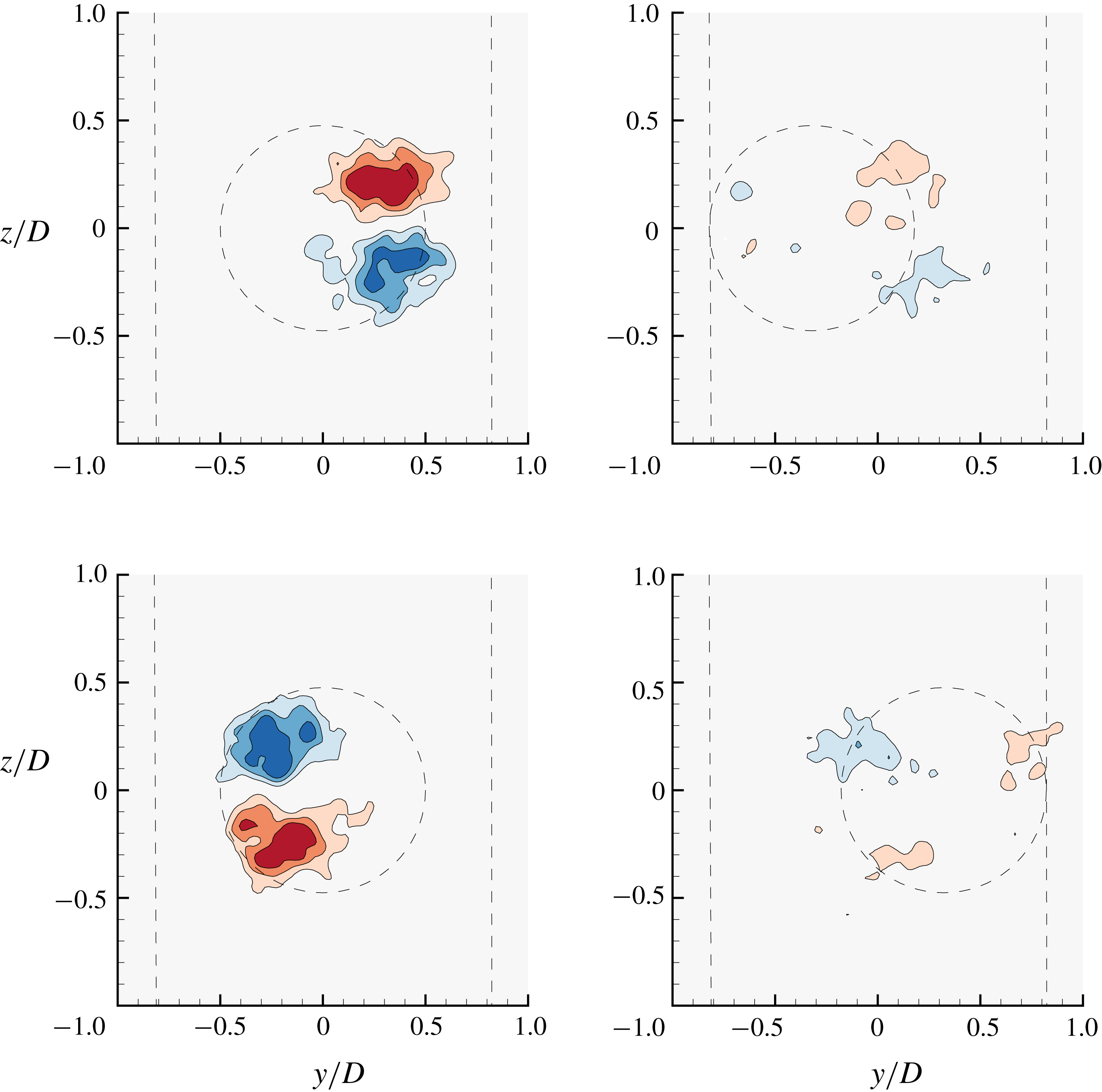
Streamwise vorticity plots showing the dominant counter-rotating vortex pair in mode I (
 $U^{\ast }=6$
) for
 $f_{R}=1.1$
during the lock-on phenomenon. Refer to figure 21 for further details.

Three-dimensional spatio-temporal reconstruction of the sphere wake based on phase-averaged streamwise vorticity (crossing the transverse plane at a distance
 $1.5D$
from the sphere rear surface) for (a)
 $f_{R}=0$
and (b)
 $f_{R}=1.1$
and
 $\unicode[STIX]{x1D6FC}_{R}=1$
in the lock-in regime. The wake is shown for mode I (
 $U^{\ast }=6$
), corresponding to a Reynolds number of
 ${\sim}8000$
. Blue indicates anti-clockwise vorticity, and red clockwise vorticity (both in the
 $x$
-
 $y$
plane). The figure clearly shows that the dominant wake structures remain the same for both the cases; however, there is a clear change in the timing of vortex shedding for
 $f_{R}=1.1$
compared to
 $f_{R}=0$
.

When the streamwise vorticity for another lock-in frequency of
 $f_{R}=1.1$
is examined as shown in figure 23, a drastic change in the vortex formation timing is clearly evident. The plots are exactly
 $180^{\circ }$
out of phase with the plots shown in figure 21 for a non-rotating sphere. This is congruent with the data reported in figure 4, where one can clearly see that
 $\unicode[STIX]{x1D719}_{total}$
jumps from
 ${\sim}0^{\circ }$
to
 $180^{\circ }$
as
 $f_{R}$
increases from
 $f_{R}=1$
to
 $f_{R}=1.1$
in the lock-on range. To provide a better perspective on the wake structures, spatio-temporal reconstructions of the sphere wake were generated for the
 $f_{R}=1.1$
case and compared to the
 $f_{R}=0$
case, as shown in figure 24(b) and figure 24(a). The spatio-temporal reconstruction was generated from 24 cross-stream vorticity fields, each phase-averaged for more than 100 cycles. A convection velocity of
 $U$
(free-stream velocity) was assumed to build the 3-D image. As evident in this case, the wake consists of an alternating two-sided chain of vortex loops, similar to the wake of an oscillating sphere with no imposed rotation reported by Govardhan & Williamson (Reference Govardhan and Williamson2005) and Sareen et al. (Reference Sareen, Zhao, Sheridan, Hourigan and Thompson2018b
). Of course, this reconstruction should not be viewed as a typical image of the wake, since it is only representative of the average wake behaviour as it passes through a fixed downstream plane.
Streamwise vorticity plots showing the dominant counter-rotating vortex pair in mode I (
 $U^{\ast }=6$
) for a frequency ratio of
 $f_{R}=1.0$
under resonance. Refer to figure 21 for further details.

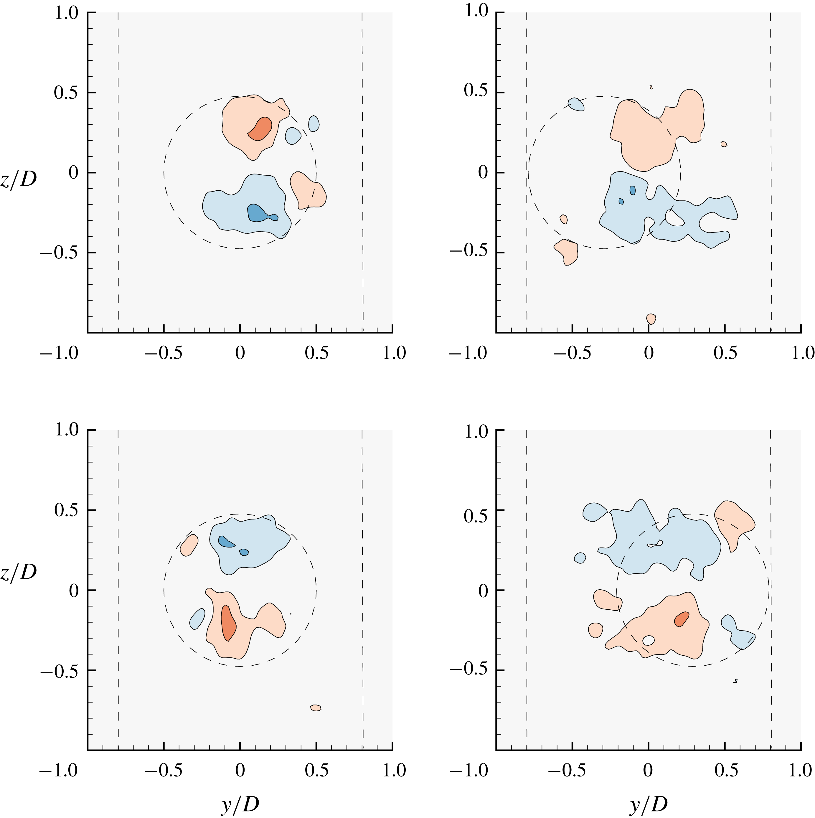
Streamwise vorticity plots showing the dominant counter-rotating vortex pair in mode I (
 $U^{\ast }=6$
) for
 $f_{R}=3$
. Refer to figure 21 for further details.

On the other hand, the streamwise vorticity plot for
 $f_{R}=1$
, as shown in figure 25, is similar to that for a sphere without any imposed rotation; there is seen to be a similar timing of vortex (loop) shedding. Again, this is consistent with the data reported in figure 4. One can conclude here that there is a change in the timing of vortex formation as the vortex shedding locks to
 $f_{R}$
with no appreciable change in the vortex structures. The streamwise vorticity field consists of a counter-rotating vortex pair which flips sign as the sphere traverses from one side to the other, as for the wake of a sphere with no imposed rotation. Another interesting case to examine is that of higher frequency ratios (
 $f_{R}>2$
), where the vibrations lock in to
 $f_{nw}$
again and the amplitude response recovers. Figure 26 shows streamwise vorticity plots for
 $f_{R}=3$
for the same parameters discussed earlier for other cases. The timing of vortex formation is similar to that for the non-rotating case. However, there is an evident reduction in the streamwise vorticity in this case. As also shown in figure 4, the vibration amplitude and the total transverse force coefficient are smaller than for the non-rotating case. Therefore, it can be concluded here that although the vibration frequency reverts to locking in to
 $f_{nw}$
instead of
 $f_{r}$
in this case, a reduction in the vibration amplitude could still be observed due to the reduction in the streamwise vorticity, in turn leading to a lower total transverse force acting on the sphere. The effect of high
 $f_{R}$
is more pronounced in mode II and mode III, where the vibrations were highly suppressed, as shown in figures 9 and 10.
6 Conclusions
A comprehensive series of experiments and wake measurements were performed to examine the effect of imposed rotary oscillation on the FIV of a sphere that is elastically mounted in the cross-flow direction. The response was investigated for a wide range of forcing parameters, non-dimensional forcing frequency,
 $f_{R}$
, in the range
 $0\leqslant f_{R}\leqslant 5$
, forcing amplitude,
 $\unicode[STIX]{x1D6FC}_{R}$
, in the range
 $0\leqslant \unicode[STIX]{x1D6FC}_{R}\leqslant 2$
, and reduced velocity
 $U^{\ast }$
between
 $0\leqslant U^{\ast }\leqslant 20$
. It was found that when the forcing frequency
 $f_{r}$
was in close proximity to the natural frequency
 $f_{nw}$
, the vibrations locked on to
 $f_{r}$
instead of
 $f_{nw,l}$
inhibiting the resonance response. The vibrations were greatly suppressed in the lock-on region, except for the case when
 $f_{R}=f_{nw}$
, where an ‘enhanced resonance’ response was observed leading to very large amplitudes, even greater than those observed for the non-rotating sphere in some cases. In the lock-on region, a sudden jump in the total phase was observed from
 $0^{\circ }$
to
 $180^{\circ }$
. The displacement signal was highly modulated in the non-lock-on regions. Near the lock-on boundaries, a wide spectrum of frequencies was observed. Interestingly, suppression was also observed in the non-lock-on regions for very high
 $f_{R}$
and
 $\unicode[STIX]{x1D6FC}_{R}$
values. Mode I was found to be quite resistant to control, requiring very high velocity ratios for the suppression of vibrations. On the other hand, control (suppression) was most effective for mode III. Overall, relatively high velocity ratios (quantified in this paper) were required to suppress the vibrations. The width of the RLO region increased with an increase in
 $\unicode[STIX]{x1D6FC}_{R}$
for all three modes. When the reduced velocity was increased progressively, several types of responses with different characteristic behaviours were observed. For some cases, the vibration amplitudes increased monotonically with an increase in
 $U^{\ast }$
. Such vibrations have been termed ‘rotary-induced vibrations’. The phase difference between the rotary oscillations and the sphere displacement
 $\unicode[STIX]{x1D719}_{rot}$
was found to be crucial in determining the response. Monotonically decreasing
 $\unicode[STIX]{x1D719}_{rot}$
values were always associated with the monotonically increasing responses. Wake measurements performed in the cross-plane revealed structures similar to those for an oscillating sphere without imposed rotation; however, there was a change in the timing of vortex formation. For a high frequency ratio of
 $f_{R}=3$
, there was a clear reduction in the streamwise vorticity consistent with a reduced amplitude response.
Acknowledgements
A.S. acknowledges the support of a Monash Graduate Scholarship (MGS) and Monash International Postgraduate Research Scholarship (MIPRS). The research was supported by Australian Research Council Discovery Project grants DP150102879 and DP170100275. She also acknowledges the Postgraduate Publication Award (PPA). The current manuscript was revised and submitted during the award period. J.Z. also acknowledges post-doctoral salary support through the latter grants.