1 Introduction
Among the different regimes of sediment transport, bedload transport is of major importance as it represents an important contribution to river morphology evolution. Accordingly, prediction of the sediment transport rate under turbulent bedload conditions is fundamental for preventing environmental risks associated with floods and scouring. From a physical point of view, bedload transport corresponds to the dynamic response of a granular bed submitted to a fluid shear stress. In contrast to suspended load, bedload is defined as the part of the sediment load occurring close to the granular bed in which particles are in permanent or intermittent contact with the bed (Fredsøe & Deigaard Reference Fredsøe and Deigaard1992).
The sediment transport rate is usually quantified in dimensionless form using the so-called Einstein number (Einstein Reference Einstein1942),
 $Q_{s}^{\ast }=Q_{s}/[d\sqrt{(\unicode[STIX]{x1D70C}^{p}/\unicode[STIX]{x1D70C}^{f}-1)gd}]$
, where
 $Q_{s}$
represents the volumetric sediment transport rate per unit width,
 $\unicode[STIX]{x1D70C}^{p}$
and
 $\unicode[STIX]{x1D70C}^{f}$
are the particle and fluid densities,
 $g$
is the acceleration of gravity and
 $d$
is the particle diameter. In the hydraulic community the classical way to model bedload transport consists of assuming a power law relation between the Einstein number and the Shields number
 $\unicode[STIX]{x1D703}$
. The latter corresponds to the ratio of the traction force exerted by the fluid at the bed
 $\unicode[STIX]{x1D70F}^{f}d^{2}$
and the buoyant weight of a single particle
 $(\unicode[STIX]{x1D70C}^{p}-\unicode[STIX]{x1D70C}^{f})gd^{3}$
, i.e.
 $\unicode[STIX]{x1D703}=\unicode[STIX]{x1D70F}^{f}/[(\unicode[STIX]{x1D70C}^{p}-\unicode[STIX]{x1D70C}^{f})gd]$
. Given the lack of accuracy of the classical formulae (e.g. Meyer-Peter & Müller Reference Meyer-Peter and Müller1948), renewed attention has recently been given to the granular phase behaviour in bedload transport (Frey & Church Reference Frey and Church2009, Reference Frey and Church2011) from both an experimental (Mouilleron, Charru & Eiff Reference Mouilleron, Charru and Eiff2009; Hergault et al.
Reference Hergault, Frey, Métivier, Barat, Ducottet, Böhm and Ancey2010; Lajeunesse, Malverti & Charru Reference Lajeunesse, Malverti and Charru2010; Aussillous et al.
Reference Aussillous, Chauchat, Pailha, Médale and Guazzelli2013; Frey Reference Frey2014; Houssais et al.
Reference Houssais, Ortiz, Durian and Jerolmack2015) and a numerical point of view (Duran, Andreotti & Claudin Reference Duran, Andreotti and Claudin2012; Ji et al.
Reference Ji, Munjiza, Avital, Ma and Williams2013; Kidanemariam & Uhlmann Reference Kidanemariam and Uhlmann2014; Maurin et al.
Reference Maurin, Chauchat, Chareyre and Frey2015).
The granular rheology characterises the response of the granular medium, in terms of deformation rate, to a given external stress, and vice versa. It is usually given as the relation between the granular stress and strain rate tensors. In bedload transport, the granular rheology governs both the response to, and the interaction with, the fluid shear stress. Its knowledge is required for two-phase flow models in which both the fluid and solid phases are considered as continuous (Eulerian–Eulerian) (e.g. Aussillous et al. Reference Aussillous, Chauchat, Pailha, Médale and Guazzelli2013). As such, it represents an important step in the upscaling of sediment transport processes from Eulerian–Lagrangian models to Eulerian–Eulerian models, which enable numerical simulations of larger-scale problems and/or complex flow forcings.
Under bedload transport conditions, the granular medium experiences all of the granular flow regimes, from quasistatic in the sediment bed to dilute rapid granular flows in the upper sediment transport layer. The dilute rapid and dense granular flow regimes have mainly been described using the kinetic theory of granular flows and the
 $\unicode[STIX]{x1D707}(I)$
rheology respectively. The former is based on the analogy of dilute granular flows with molecular gases, assuming binary collisions. It has been proven to accurately describe rapid dilute granular flows in different configurations (Campbell Reference Campbell1990; Goldhirsch Reference Goldhirsch2003) and has recently been extended to the dense granular flow regime (Jenkins Reference Jenkins2006, Reference Jenkins2007; Berzi, di Prisco & Vescovi Reference Berzi, di Prisco and Vescovi2011). Alternatively, the
 $\unicode[STIX]{x1D707}(I)$
local rheology accurately describes the dense granular flow regimes and is based on the dimensional analysis of the simple shear configuration (Midi Reference Midi2004; Forterre & Pouliquen Reference Forterre and Pouliquen2008; Jop Reference Jop2015). In the latter case, the unique dimensionless number controlling the system is the so-called inertial number (Da Cruz et al.
Reference Da Cruz, Emam, Prochnow, Roux and Chevoir2005):
 $$\begin{eqnarray}\displaystyle I=\dot{\unicode[STIX]{x1D6FE}}d\sqrt{\unicode[STIX]{x1D70C}^{p}/\unicode[STIX]{x1D617}^{p}}, & & \displaystyle\end{eqnarray}$$
with
 $\unicode[STIX]{x1D617}^{p}$
the confining granular pressure and
 $\dot{\unicode[STIX]{x1D6FE}}$
the granular shear rate. This dimensionless number can be interpreted as the ratio between a macroscopic time scale of deformation
 $t_{macro}=1/\dot{\unicode[STIX]{x1D6FE}}$
and a microscopic time scale of rearrangement
 $t_{micro}=d/\sqrt{\unicode[STIX]{x1D617}^{p}/\unicode[STIX]{x1D70C}^{p}}$
. From the dimensional analysis, the dimensionless solid volume fraction
 $\unicode[STIX]{x1D719}$
and shear to normal granular stress ratio
 $\unicode[STIX]{x1D707}=\unicode[STIX]{x1D70F}^{p}/\unicode[STIX]{x1D617}^{p}$
are unique functions of the inertial number
 $I$
. From experiments and numerical simulations, they can be expressed as (Da Cruz et al.
Reference Da Cruz, Emam, Prochnow, Roux and Chevoir2005; Jop, Forterre & Pouliquen Reference Jop, Forterre and Pouliquen2006)
 $$\begin{eqnarray}\displaystyle & \displaystyle \frac{\unicode[STIX]{x1D70F}^{p}}{\unicode[STIX]{x1D617}^{p}}=\unicode[STIX]{x1D707}(I)=\unicode[STIX]{x1D707}_{s}+\frac{\unicode[STIX]{x1D707}_{2}-\unicode[STIX]{x1D707}_{s}}{1+I_{0}/I}, & \displaystyle\end{eqnarray}$$
 $$\begin{eqnarray}\displaystyle & \displaystyle \unicode[STIX]{x1D719}(I)=\unicode[STIX]{x1D719}^{max}-aI, & \displaystyle\end{eqnarray}$$
where
 $\unicode[STIX]{x1D719}^{max}$
is the maximum packing fraction,
 $\unicode[STIX]{x1D707}_{s}$
is the static effective granular friction coefficient, and
 $\unicode[STIX]{x1D707}_{2}$
,
 $I_{0}$
and
 $a$
are phenomenological constants. By combining the different expressions (1.1)–(1.3), the granular stress tensor can be expressed as a function of the shear rate, defining the granular rheology.
Based on the simple shear configuration, the
 $\unicode[STIX]{x1D707}(I)$
rheology has been extended to account for the presence of interstitial fluids (Courrech du Pont et al.
Reference Courrech du Pont, Gondret, Perrin and Rabaud2003; Cassar, Nicolas & Pouliquen Reference Cassar, Nicolas and Pouliquen2005). Considering rearrangement time scales according to the dominant mechanism, three regimes can be defined by introducing two dimensionless numbers (Courrech du Pont et al.
Reference Courrech du Pont, Gondret, Perrin and Rabaud2003; Cassar et al.
Reference Cassar, Nicolas and Pouliquen2005; Andreotti, Forterre & Pouliquen Reference Andreotti, Forterre and Pouliquen2013), with
 $C_{D}$
the drag coefficient,
 $$\begin{eqnarray}\displaystyle & \displaystyle St=\frac{d\sqrt{\unicode[STIX]{x1D70C}^{p}\unicode[STIX]{x1D617}^{p}}}{\unicode[STIX]{x1D702}^{f}}, & \displaystyle\end{eqnarray}$$
 $$\begin{eqnarray}\displaystyle & \displaystyle r=\sqrt{\frac{\unicode[STIX]{x1D70C}^{p}}{\unicode[STIX]{x1D70C}^{f}C_{D}}}, & \displaystyle\end{eqnarray}$$
the free-fall regime (
 $St\gg 1$
,
 $r\gg 1$
) corresponding to negligible influence of the interstitial fluid (i.e. dry granular media), the viscous regime (
 $St\ll 1$
,
 $r\ll 1$
) corresponding to a rearrangement time scale dominated by viscous drag and the turbulent regime (
 $St\gg 1$
,
 $r\ll 1$
) corresponding to a rearrangement time scale dominated by fluid inertial effects. In the different regimes, the results therefore scale with the dry inertial number
 $I_{dry}=\dot{\unicode[STIX]{x1D6FE}}d\sqrt{\unicode[STIX]{x1D70C}^{p}/\unicode[STIX]{x1D617}^{p}}$
, the turbulent one
 $I_{turb}=\dot{\unicode[STIX]{x1D6FE}}d\sqrt{\unicode[STIX]{x1D70C}^{f}C_{D}/\unicode[STIX]{x1D617}^{p}}$
and the viscous one
 $I_{visc}=\unicode[STIX]{x1D702}^{f}\dot{\unicode[STIX]{x1D6FE}}/\unicode[STIX]{x1D617}^{p}$
respectively. This approach has been applied with some success to various complex immersed configurations from avalanches (Courrech du Pont et al.
Reference Courrech du Pont, Gondret, Perrin and Rabaud2003; Cassar et al.
Reference Cassar, Nicolas and Pouliquen2005; Doppler et al.
Reference Doppler, Gondret, Loiseleux, Meyer and Rabaud2007), to granular collapses (Rondon, Pouliquen & Aussillous Reference Rondon, Pouliquen and Aussillous2011; Izard, Bonometti & Lacaze Reference Izard, Bonometti and Lacaze2014), annular shear cells (Boyer, Guazzelli & Pouliquen Reference Boyer, Guazzelli and Pouliquen2011; Trulsson, Andreotti & Claudin Reference Trulsson, Andreotti and Claudin2012) and sediment transport (Ouriemi, Aussillous & Guazzelli Reference Ouriemi, Aussillous and Guazzelli2009; Aussillous et al.
Reference Aussillous, Chauchat, Pailha, Médale and Guazzelli2013; Revil-Baudard & Chauchat Reference Revil-Baudard and Chauchat2013; Chiodi, Claudin & Andreotti Reference Chiodi, Claudin and Andreotti2014).
To the best of our knowledge, there are only a few contributions in the literature on the dense granular flow rheology in the context of bedload transport. Ouriemi et al. (Reference Ouriemi, Aussillous and Guazzelli2009) and Aussillous et al. (Reference Aussillous, Chauchat, Pailha, Médale and Guazzelli2013) have studied laminar bedload in closed conducts using refractive index-matching experiments and theoretical two-phase continuous models. Assuming a constant solid volume fraction and a limited transitional layer from dense to dilute granular flow, the authors have shown that the
 $\unicode[STIX]{x1D707}(I)$
rheology gives excellent agreement with experimental data. It is worth noting that in the laminar case, the lag between the fluid and solid velocities is negligible (Mouilleron et al.
Reference Mouilleron, Charru and Eiff2009; Aussillous et al.
Reference Aussillous, Chauchat, Pailha, Médale and Guazzelli2013), the two phases being tightly coupled. In intense turbulent bedload transport, termed sheet flow, the transitional layer from dense to dilute granular flows and the fluid–particle velocity lag are more important (Sumer et al.
Reference Sumer, Kozakiewicz, Fredsøe and Deigaard1996; Cowen et al.
Reference Cowen, Dudley, Liao, Variano and Liu2010; Revil-Baudard et al.
Reference Revil-Baudard, Chauchat, Hurther and Barraud2015). This regime has been studied experimentally (Capart & Fraccarollo Reference Capart and Fraccarollo2011) and numerically using the two-phase flow continuous modelling framework with the kinetic theory of granular flows (Jenkins & Hanes Reference Jenkins and Hanes1998; Hsu, Jenkins & Liu Reference Hsu, Jenkins and Liu2004) and the
 $\unicode[STIX]{x1D707}(I)$
rheology (Revil-Baudard & Chauchat Reference Revil-Baudard and Chauchat2013; Chauchat, Revil-Baudard & Hurther Reference Chauchat, Revil-Baudard and Hurther2015). While the agreement of the numerical simulations with the available experimental data gives some credit to both granular rheologies, recent experimental investigations by Revil-Baudard et al. (Reference Revil-Baudard, Chauchat, Hurther and Barraud2015) showed that the solid volume fraction profiles observed were substantially different from the predicted ones. The observed effective friction coefficient also differs importantly from the classical values used in the
 $\unicode[STIX]{x1D707}(I)$
rheology, possibly due to the strong intermittency induced by the turbulent coherent structures (Revil-Baudard et al.
Reference Revil-Baudard, Chauchat, Hurther and Barraud2015). At the transition from sheet flows to debris flow, the granular rheology has been used to model steep slope configurations (Armanini et al.
Reference Armanini, Capart, Fraccarollo and Larcher2005; Larcher et al.
Reference Larcher, Fraccarollo, Armanini and Capart2007; Berzi & Jenkins Reference Berzi and Jenkins2008; Armanini et al.
Reference Armanini, Larcher, Nucci and Dumbser2014). Combining experimental particle tracking at the wall (Armanini et al.
Reference Armanini, Capart, Fraccarollo and Larcher2005; Larcher et al.
Reference Larcher, Fraccarollo, Armanini and Capart2007) and numerical analysis (Berzi & Jenkins Reference Berzi and Jenkins2008; Armanini et al.
Reference Armanini, Larcher, Nucci and Dumbser2014), both the
 $\unicode[STIX]{x1D707}(I)$
rheology (Berzi & Jenkins Reference Berzi and Jenkins2008) and hybrid
 $\unicode[STIX]{x1D707}(I)$
–kinetic-theory models (Armanini et al.
Reference Armanini, Larcher, Nucci and Dumbser2014) have been shown to accurately describe the granular behaviour in this configuration.
The literature review underlines the relevance of both the kinetic theory and the dense granular flow rheology for bedload transport modelling. However, the numerical studies are restricted to continuous two-phase analysis and the experimental evaluations of the granular stress tensor rely on solid volume fraction measurements that are highly uncertain. In addition, while direct numerical simulations (DNS) have been performed at the particle scale in the laminar regime (Kidanemariam & Uhlmann Reference Kidanemariam and Uhlmann2014), this type of numerical model is not affordable for turbulent bedload transport due to the typical values of bulk Reynolds numbers explored. Therefore, to go beyond the existing two-phase continuous numerical works, the present paper analyses the local granular rheology in turbulent bedload transport using a coupled fluid–discrete-element model (DEM) with a volume-averaged fluid description (Maurin et al. Reference Maurin, Chauchat, Chareyre and Frey2015). This approach permits local computation of the granular stress tensor and the granular shear rate, bringing new insights into the local granular behaviour in turbulent bedload transport. Based on these Eulerian–Lagrangian simulations a dense granular flow rheology for bedload transport is proposed and further tested in a two-phase continuous (Eulerian–Eulerian) model. Besides, bedload transport configurations enable local analysis of the granular rheology in complex immersed granular flows, and the DEM results are shown to be of interest for granular media in general.
The paper is structured as follows. First, the coupled fluid–DEM and two-phase continuous models are briefly presented (§ 2). Then, fluid–DEM simulations are analysed in the framework of the dense granular flow
 $\unicode[STIX]{x1D707}(I)$
rheology (§ 3). Finally, extending the simulations to realistic conditions for bedload transport, a parametrisation of the
 $\unicode[STIX]{x1D707}(I)$
rheology is proposed from the DEM results, and is tested with the two-phase continuous model (§ 4).
2 Model formulation
The Eulerian–Lagrangian and Eulerian–Eulerian models are based on the same volume-averaged two-phase flow equations for the fluid phase. The solid phase is modelled on the one hand as a continuum (Eulerian–Eulerian) and on the other hand using a 3D DEM in which each particle motion is computed explicitly (Eulerian–Lagrangian). Both two-phase flow models have already been described and validated with experiments (Chauchat et al. Reference Chauchat, Revil-Baudard and Hurther2015; Maurin et al. Reference Maurin, Chauchat, Chareyre and Frey2015), and only a brief description will be given. The reader is referred to the abovementioned references for a complete description of the model formulations and validations.
Considering steady uniform conditions, the problem is unidirectional, so that the average fluid and solid velocities depend only on the wall-normal direction and reduce to their streamwise components
 $\langle \boldsymbol{u}\rangle ^{f}=\langle u_{x}\rangle ^{f}(z)\boldsymbol{e}_{\boldsymbol{x}}$
and
 $\langle \boldsymbol{v}^{p}\rangle ^{s}=\langle v_{x}^{p}\rangle ^{s}(z)\boldsymbol{e}_{\boldsymbol{x}}$
. Therefore, the streamwise and wall-normal volume-averaged fluid phase momentum balances are given by (Anderson & Jackson Reference Anderson and Jackson1967; Jackson Reference Jackson2000; Revil-Baudard & Chauchat Reference Revil-Baudard and Chauchat2013)
 $$\begin{eqnarray}\displaystyle & \displaystyle 0=\frac{\unicode[STIX]{x2202}S_{xz}^{\,f}}{\unicode[STIX]{x2202}z}+\frac{\unicode[STIX]{x2202}\unicode[STIX]{x1D619}_{xz}^{\,f}}{\unicode[STIX]{x2202}z}+\unicode[STIX]{x1D70C}^{f}(1-\unicode[STIX]{x1D719})g\sin \unicode[STIX]{x1D6FC}-n\langle f_{x}\rangle ^{p}, & \displaystyle\end{eqnarray}$$
 $$\begin{eqnarray}\displaystyle & \displaystyle 0=-\frac{\unicode[STIX]{x2202}\unicode[STIX]{x1D617}^{\,f}}{\unicode[STIX]{x2202}z}+\unicode[STIX]{x1D70C}^{f}(1-\unicode[STIX]{x1D719})g\cos \unicode[STIX]{x1D6FC}-n\langle f_{z}\rangle ^{p}, & \displaystyle\end{eqnarray}$$
where
 $\unicode[STIX]{x1D70E}_{ij}^{f}=-\unicode[STIX]{x1D617}^{\,f}\unicode[STIX]{x1D6FF}_{ij}+S_{ij}^{\,f}$
is the volume-averaged effective viscous stress tensor,
 $\unicode[STIX]{x1D619}_{xz}^{\,f}$
is the Reynolds shear stress tensor,
 $\unicode[STIX]{x1D719}$
is the solid phase volume fraction,
 $\langle f_{k}\rangle ^{p}$
is the volume-averaged fluid–particle interaction force,
 $n=\unicode[STIX]{x1D719}/(\unicode[STIX]{x03C0}d^{3}/6)$
is the number density of particles and
 $\unicode[STIX]{x1D6FC}$
is the channel inclination angle. Omitting the model-dependent fluid–particle interaction force, the solution of the fluid momentum balance requires closure laws for the viscous shear stress tensor and the Reynolds stress tensor.
Considering a Newtonian fluid, the viscous shear stress is classically expressed as
 $$\begin{eqnarray}\displaystyle \unicode[STIX]{x1D61A}_{xz}^{\,f}=\unicode[STIX]{x1D70C}^{f}(1-\unicode[STIX]{x1D719})\unicode[STIX]{x1D708}^{f}\frac{\text{d}\langle u_{x}\rangle ^{f}}{\,\text{d}z}, & & \displaystyle\end{eqnarray}$$
with
 $\unicode[STIX]{x1D708}^{f}$
the clear fluid kinematic viscosity and
 $\langle u_{x}\rangle ^{f}$
the volume-averaged streamwise fluid phase velocity. The Reynolds shear stress is based on the eddy viscosity concept (
 $\unicode[STIX]{x1D708}^{t}$
) using a mixing length formulation:
 $$\begin{eqnarray}\displaystyle \unicode[STIX]{x1D619}_{xz}^{\,f}=\unicode[STIX]{x1D70C}^{f}~\unicode[STIX]{x1D708}^{t}\frac{\text{d}\langle u_{x}\rangle ^{f}}{\,\text{d}z},\quad \text{with }\unicode[STIX]{x1D708}^{t}=(1-\unicode[STIX]{x1D719})l_{m}^{2}\left|\frac{\text{d}\langle u_{x}\rangle ^{f}}{\,\text{d}z}\right|, & & \displaystyle\end{eqnarray}$$
where the mixing length is taken similarly to Li & Sawamoto (Reference Li and Sawamoto1995) as
 $$\begin{eqnarray}\displaystyle l_{m}(z)=\unicode[STIX]{x1D705}\int _{0}^{z}\frac{\unicode[STIX]{x1D719}^{max}-\unicode[STIX]{x1D719}(\unicode[STIX]{x1D701})}{\unicode[STIX]{x1D719}^{max}}\,\text{d}\unicode[STIX]{x1D701}, & & \displaystyle\end{eqnarray}$$
with
 $\unicode[STIX]{x1D705}=0.41$
the von Karman constant. The formulation adopted allows one to recover the law of the wall (Prandtl Reference Prandtl1926) in clear fluid, while the turbulence is completely damped inside the granular bed at maximum packing fraction (
 $\unicode[STIX]{x1D719}^{max}$
).
2.1 Eulerian–Lagrangian model
The Eulerian–Lagrangian model is based on the explicit solution of the dynamic equation for each individual particle using the 3D DEM open-source code YADE (Šmilauer et al.
Reference Šmilauer, Catalano, Chareyre, Dorofeenko, Duriez, Dyck, Elias, Er, Eulitz and Gladky2015). The DEM solution is spatially averaged and explicitly coupled with the fluid phase momentum balance equations (2.1)–(2.2) through the drag term
 $n\langle f_{x}^{D}\rangle ^{p}$
and the solid volume fraction
 $\unicode[STIX]{x1D719}$
.
For each particle
 $p$
at position
 $\boldsymbol{x}^{p}$
, the Newton equations are solved considering nearest-neighbours interactions:
 $$\begin{eqnarray}\displaystyle m\frac{\text{d}^{2}\boldsymbol{x}^{p}}{\text{d}t^{2}}=\mathop{\sum }_{k\in \mathscr{N}}\boldsymbol{f}_{c}^{pk}+\boldsymbol{f}_{ext}=\mathop{\sum }_{k\in \mathscr{N}}\boldsymbol{f}_{c}^{pk}+\boldsymbol{f}_{g}^{p}+\boldsymbol{f}_{b}^{p}+\boldsymbol{f}_{D}^{p}, & & \displaystyle\end{eqnarray}$$
where the sum of the contact forces
 $\boldsymbol{f}_{c}^{pk}$
is made over the ensemble of nearest neighbours
 $\mathscr{N}$
,
 $\boldsymbol{f}_{g}^{p}$
is the gravity force,
 $\boldsymbol{f}_{b}^{p}$
is the buoyancy force and
 $\boldsymbol{f}_{D}^{p}$
is the 3D drag force applied by the fluid on particle
 $p$
. For each contact, the contact force is computed explicitly using the classical spring–dashpot contact law (Schwager & Pöschel Reference Schwager and Pöschel2007):
 $$\begin{eqnarray}\displaystyle & \displaystyle F_{n}=-k_{n}\unicode[STIX]{x1D6FF}_{n}-c_{n}\dot{\unicode[STIX]{x1D6FF}_{n}}, & \displaystyle\end{eqnarray}$$
 $$\begin{eqnarray}\displaystyle & \displaystyle F_{t}=-\min (k_{s}\unicode[STIX]{x1D6FF}_{t},\unicode[STIX]{x1D707}^{p}F_{n}), & \displaystyle\end{eqnarray}$$
 $F_{n}$
and
 $F_{t}$
are the normal and tangential contact forces between particle
 $p$
and
 $k$
,
 $\unicode[STIX]{x1D6FF}_{n}$
and
 $\unicode[STIX]{x1D6FF}_{t}$
are the normal and tangential overlaps,
 $k_{n}$
and
 $k_{s}$
are the normal and tangential contact stiffnesses,
 $c_{n}$
is the normal viscous damping and
 $\unicode[STIX]{x1D707}^{p}$
is the tangential friction coefficient. This contact law is well suited for granular flow analysis and allows one to define a unique restitution coefficient
 $e_{n}$
(Schwager & Pöschel Reference Schwager and Pöschel2007). Similarly, the rotation of the particles is solved from the Newton equations of motion.
The interaction with the fluid phase is restricted to buoyancy and drag forces:
 $$\begin{eqnarray}\displaystyle & \displaystyle \boldsymbol{f}_{b}^{p}=-\frac{\unicode[STIX]{x03C0}d^{3}}{6}\unicode[STIX]{x1D735}\unicode[STIX]{x1D617}^{\,f}, & \displaystyle\end{eqnarray}$$
 $$\begin{eqnarray}\displaystyle & \displaystyle \boldsymbol{f}_{D}^{p}=\frac{1}{2}\unicode[STIX]{x1D70C}^{f}\frac{\unicode[STIX]{x03C0}d^{2}}{4}C_{D}\Vert \langle \boldsymbol{u}\rangle _{\boldsymbol{x}^{\boldsymbol{p}}}^{f}-\boldsymbol{v}^{\boldsymbol{p}}\Vert (\langle \boldsymbol{u}\rangle _{\boldsymbol{x}^{\boldsymbol{p}}}^{f}-\boldsymbol{v}^{\boldsymbol{p}}), & \displaystyle\end{eqnarray}$$
where the average fluid velocity and the fluid pressure are taken at the centre of particle
 $p$
. The drag coefficient
 $C_{D}$
depends on the particle Reynolds number
 $Re_{p}=\Vert \langle \boldsymbol{u}\rangle _{\boldsymbol{x}^{\boldsymbol{p}}}^{f}-\boldsymbol{v}^{\boldsymbol{p}}\Vert d/\unicode[STIX]{x1D708}^{f}$
and takes into account hindrance effects (DallaValle Reference Dallavalle1948; Richardson & Zaki Reference Richardson and Zaki1954):
 $C_{D}=(0.4+24.4/Re_{p})(1-\unicode[STIX]{x1D719})^{-3.1}$
.
Considering steady uniform turbulent flows, the buoyancy force reduces to its wall-normal component and (2.2) leads to a hydrostatic fluid pressure distribution, the wall-normal average drag force being negligible. The solution of the streamwise fluid phase momentum balance (2.1) requires the evaluation of both the spatially averaged solid phase volume fraction and the momentum transmitted from the fluid to the particles through drag forces:
 $$\begin{eqnarray}\displaystyle n\langle f_{x}^{D}\rangle ^{s}=\frac{\unicode[STIX]{x1D719}}{\unicode[STIX]{x03C0}d^{3}/6}\langle f_{x}^{D}\rangle ^{s}=\frac{3}{4}\frac{\unicode[STIX]{x1D719}\unicode[STIX]{x1D70C}^{f}}{d}\langle C_{D}\Vert \langle \boldsymbol{u}\rangle ^{f}-\boldsymbol{v}^{\boldsymbol{p}}\Vert (\langle u_{x}\rangle ^{f}-v_{x}^{p})\rangle ^{s}. & & \displaystyle\end{eqnarray}$$
In the DEM processing, the solid phase averaging
 $\langle \bullet \rangle ^{s}$
is used instead of the particle phase averaging
 $\langle \bullet \rangle ^{p}$
. While the two are identical provided that there is scale separation (Anderson & Jackson Reference Anderson and Jackson1967; Jackson Reference Jackson2000), the importance of the wall-normal gradients in bedload transport requires a weighting function length scale lower than the particle diameter in order to define an independent averaging (Maurin Reference Maurin2015; Maurin et al.
Reference Maurin, Chauchat, Chareyre and Frey2015). Therefore, a small wall-normal weighting function length scale has been adopted (typically
 $d/30$
), and this choice has been validated through an experimental comparison (Maurin et al.
Reference Maurin, Chauchat, Chareyre and Frey2015).
The 3D DEM and the fluid model are solved as transient problems applying a fixed bottom boundary condition for both the fluid (
 $\langle \boldsymbol{u}\rangle ^{f}(z=0)=0$
) and the particle phase (fixed random particles) and imposing the position of the water free surface (
 $\text{d}\langle u_{x}\rangle ^{f}/\text{d}z(z=h)=0$
). In order to achieve a stable integration, the DEM time step is bounded by the propagation time of the fastest wave over a particle diameter (Maurin Reference Maurin2015; Maurin et al.
Reference Maurin, Chauchat, Chareyre and Frey2015). The fluid resolution time step corresponds to a typical characteristic evolution time scale of the granular medium and is taken much larger than the DEM one (Maurin et al.
Reference Maurin, Chauchat, Chareyre and Frey2015):
 $\unicode[STIX]{x0394}t_{f}=10^{-2}~\text{s}$
with respect to
 $\unicode[STIX]{x0394}t_{p}\sim O(10^{-4}{-}10^{-5})~\text{s}$
. Therefore, the coupling between the fluid and granular phases ensures momentum conservation of the system on average. The model has been compared with experiments and has shown its ability to describe accurately the granular depth structure in turbulent bedload transport (Maurin et al.
Reference Maurin, Chauchat, Chareyre and Frey2015).
2.2 Eulerian–Eulerian model
The Eulerian–Eulerian model is based on the numerical solution of the fluid phase momentum balance equations (2.1) and (2.2) coupled with the spatially averaged granular phase momentum balance equations in the streamwise and wall-normal directions. For steady uniform flow conditions the granular phase momentum equations read (Chauchat et al. Reference Chauchat, Revil-Baudard and Hurther2015)
 $$\begin{eqnarray}\displaystyle 0=\frac{\unicode[STIX]{x2202}\unicode[STIX]{x1D70F}_{xz}^{p}}{\unicode[STIX]{x2202}z}+\unicode[STIX]{x1D70C}^{p}\unicode[STIX]{x1D719}g\sin \unicode[STIX]{x1D6FC}+n\langle f_{x}\rangle ^{p}, & & \displaystyle\end{eqnarray}$$
 $$\begin{eqnarray}\displaystyle 0=-\frac{\unicode[STIX]{x2202}\unicode[STIX]{x1D617}^{p}}{\unicode[STIX]{x2202}z}+\unicode[STIX]{x1D70C}^{p}\unicode[STIX]{x1D719}g\cos \unicode[STIX]{x1D6FC}+n\langle f_{z}\rangle ^{p}, & & \displaystyle\end{eqnarray}$$
where
 $\unicode[STIX]{x1D70F}_{xz}^{p}$
is the spatially averaged granular phase shear stress. Like in the Eulerian–Lagrangian model, the buoyancy is applied along the wall-normal direction and leads to hydrostatic pressure distribution for the granular phase. In the continuous formalism the spatially averaged streamwise drag force is given by
 $$\begin{eqnarray}\displaystyle n\langle \boldsymbol{f}^{D}\rangle ^{s}=\frac{3}{4}\frac{\unicode[STIX]{x1D719}\unicode[STIX]{x1D70C}^{f}}{d}C_{D}\Vert \langle \boldsymbol{u}\rangle ^{f}-\langle \boldsymbol{v}^{\boldsymbol{p}}\rangle ^{s}+\boldsymbol{u}_{\boldsymbol{ d}}\Vert (\langle \boldsymbol{u}\rangle ^{f}-\langle \boldsymbol{v}^{\boldsymbol{p}}\rangle ^{s}+\boldsymbol{u}_{\boldsymbol{ d}}), & & \displaystyle\end{eqnarray}$$
where the extra term
 $\boldsymbol{u}_{\boldsymbol{d}}$
is the drift velocity which represents the dispersion effect due to the averaged fluid–particle velocity fluctuations. This term is responsible for sediment transport suspension and allows one to reproduce the Rouse profile provided that the wall-normal component is taken as
 $(u_{d})_{z}=-\unicode[STIX]{x1D708}^{t}/\unicode[STIX]{x1D719}~\text{d}\unicode[STIX]{x1D719}/\text{d}z$
(Chauchat et al.
Reference Chauchat, Revil-Baudard and Hurther2015). The streamwise component is taken as
 $(u_{d})_{x}=0$
in this paper.
The granular shear stress tensor is modelled using the
 $\unicode[STIX]{x1D707}(I)$
rheology presented in the introduction. Combining equations (1.1) and (1.2), the shear and normal components of the granular stress tensor can be expressed as
 $$\begin{eqnarray}\displaystyle \displaystyle \unicode[STIX]{x1D617}^{p}=\frac{1}{I^{2}}\unicode[STIX]{x1D70C}_{p}\,d^{2}\left(\frac{\text{d}\langle v_{x}^{p}\rangle ^{s}}{\text{d}z}\right)^{2}, & & \displaystyle\end{eqnarray}$$
 $$\begin{eqnarray}\displaystyle \displaystyle \unicode[STIX]{x1D70F}^{p}=\frac{\unicode[STIX]{x1D707}(I)}{I^{2}}\unicode[STIX]{x1D70C}_{p}\,d^{2}\left(\frac{\text{d}\langle v_{x}^{p}\rangle ^{s}}{\text{d}z}\right)^{2}. & & \displaystyle\end{eqnarray}$$
Inverting equation (1.3), the inertial number is obtained as a function of the solid volume fraction, and the two equations can be directly expressed as a function of the solid volume fraction and the average solid velocity gradient.
The numerical algorithm is based on a transient solution of the governing equations (2.1), (2.2), (2.11) and (2.12), together with the continuity equation for the solid phase. Fixed boundary conditions are imposed at the bottom of the sample at
 $z=0$
(
 $\langle \boldsymbol{u}\rangle ^{f}=0$
) where the granular phase is considered to be at rest (
 $\langle \boldsymbol{v}^{p}\rangle ^{s}=0$
,
 $\text{d}\unicode[STIX]{x1D719}/\text{d}z=0$
), while the positions of the water and granular free surfaces are imposed at
 $z=h$
(
 $\text{d}\langle u_{x}\rangle ^{f}/\text{d}z=0$
,
 $\langle u_{z}\rangle ^{f}=0$
,
 $\langle v_{z}^{p}\rangle ^{s}=0$
,
 $\text{d}\unicode[STIX]{x1D719}/\text{d}z=0$
). The governing equations are discretised using a finite volume technique for the mass conservation equation and a finite difference technique for the momentum balance. A staggered grid is used with the velocities located at the cell face and the scalar quantities (e.g. volume fractions or viscosities) located at the cell centre. For the pressure–velocity coupling a projection method is used. The numerical schemes are Euler implicit for the time derivative, upwind for the advection terms and central difference for the diffusion terms. For additional informations on the numerical model, the reader is referred to Chauchat et al. (Reference Chauchat, Guillou, Pham Van Bang and Dan Nguyen2013) and Chauchat et al. (Reference Chauchat, Revil-Baudard and Hurther2015).
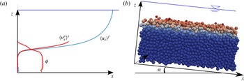
Scheme of the numerical set-up and its equivalent average unidirectional picture with typical fluid velocity
 $\langle \boldsymbol{u}^{f}\rangle =\langle u_{x}^{f}\rangle (z)\boldsymbol{e}_{\boldsymbol{x}}$
, solid volume fraction
 $\unicode[STIX]{x1D719}$
and solid velocity
 $\langle \boldsymbol{v}\rangle ^{s}=\langle v_{x}\rangle ^{s}(z)\boldsymbol{e}_{\boldsymbol{x}}$
depth profiles. The inclined 3D biperiodic granular description is coupled with a unidirectional fluid momentum balance using imposed fixed random bottom boundary condition and water free-surface position. The particle colour is representative of the velocity intensity.

3 Results and methodology
The numerical set-up of the Eulerian–Lagrangian model is presented in figure 1. It consists of a channel flow tilted with an inclination angle
 $\unicode[STIX]{x1D6FC}=0.05$
rad, partially filled with monodisperse spherical particles of diameter
 $d$
. The three-dimensional granular sample is biperiodic (streamwise and spanwise) and the periodic cell size is taken as
 $l_{x}=l_{y}=30d$
to ensure statistical convergence of the spatial averaging operator (Maurin et al.
Reference Maurin, Chauchat, Chareyre and Frey2015). A 10–15 diameter thick granular layer is deposited under gravity over a rough random bottom, and the system evolves under gravity with a fixed water free-surface elevation. The water flow is turbulent (
 $Re=U^{f}h/\unicode[STIX]{x1D708}^{f}\sim 10^{4}$
), hydraulically rough (
 $Re_{p}=U^{f}d/\unicode[STIX]{x1D708}^{f}\sim 10^{3}$
) and supercritical (
 $Fr=U^{f}/\sqrt{gh}\gtrsim 1$
), with
 $U^{f}$
the average fluid velocity within the water depth
 $h$
. The results are independent of the granular bottom boundary conditions in the range of parameters investigated (Maurin Reference Maurin2015) and the simulations are performed in the rigid grain limit (Roux & Combe Reference Roux and Combe2002) with a tangential stiffness set to half the normal one. The friction coefficient is set to a realistic value for glass beads,
 $\unicode[STIX]{x1D707}^{p}=0.4$
, and the restitution coefficient is taken as
 $e_{n}=0.5$
to account for the lubrication effect consistently with the experimental validation (Maurin et al.
Reference Maurin, Chauchat, Chareyre and Frey2015).
In order to define properly an equivalent continuous medium for the granular phase, the analysis is restricted, in a first approach, to cases with a non-negligible number of particle layers in motion. The range of Shields numbers investigated has been chosen between
 $\unicode[STIX]{x1D703}^{\ast }\sim 0.2$
and
 $\unicode[STIX]{x1D703}^{\ast }\sim 0.6$
, to prevent suspended load and stay in the bedload regime by keeping high suspension numbers (
 $S^{\ast }=w_{s}/u_{\ast }\in [2,5]$
). For mountain stream bedload, this represents intense rare events with high transport capacity. It can also be seen as a limit case of sheet flow without suspension. In order to investigate the scaling laws, the Shields number, the specific density and the particle diameter are varied. For each parameter, three values are considered starting from a realistic case for intense bedload transport (
 $\unicode[STIX]{x1D703}^{\ast }\sim 0.4$
,
 $\unicode[STIX]{x1D70C}^{p}/\unicode[STIX]{x1D70C}^{f}-1=1.5$
,
 $d=6$
mm), corresponding to the particle density and diameter used for the experimental validation (Maurin et al.
Reference Maurin, Chauchat, Chareyre and Frey2015). The specific density is lowered starting from
 $\unicode[STIX]{x1D70C}^{p}/\unicode[STIX]{x1D70C}^{f}-1=1.5$
, considering that experiments are often realized using plastic particles in sheet flows (e.g. Capart & Fraccarollo Reference Capart and Fraccarollo2011; Revil-Baudard et al.
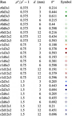
Reference Revil-Baudard, Chauchat, Hurther and Barraud2015). The main characteristic dimensionless numbers of the problem are shown in table 1 and the exact parameters investigated are given in table 2. For each run, once the system is at steady state, the data measured every 0.1 s are averaged over time for 300 s for post-processing.
3.1 Methodology
In order to study the granular rheology, the granular stress tensor is computed from the 3D DEM results by applying the spatial averaging operator to the granular stress tensor. Therefore,
 $\langle \unicode[STIX]{x1D70E}_{ij}^{p}\rangle ^{s}$
is obtained for each slice of volume
 $V$
by computing (Goldhirsch Reference Goldhirsch2010; Andreotti et al.
Reference Andreotti, Forterre and Pouliquen2013)
 $$\begin{eqnarray}\displaystyle \langle \unicode[STIX]{x1D70E}_{ij}^{p}\rangle ^{s}=-\unicode[STIX]{x1D617}^{p}\unicode[STIX]{x1D6FF}_{ij}+\unicode[STIX]{x1D70F}_{ij}^{p}=-\frac{1}{V}\mathop{\sum }_{\unicode[STIX]{x1D6FD}\in V}m^{\unicode[STIX]{x1D6FD}}v_{i}^{\prime \unicode[STIX]{x1D6FD}}v_{j}^{\prime \unicode[STIX]{x1D6FD}}-\frac{1}{V}\mathop{\sum }_{(m,n)\in V}f_{c,i}^{m,n}b_{j}^{m,n}, & & \displaystyle\end{eqnarray}$$
where the sums are respectively over the particles and the contacts contained in the volume
 $V$
,
 $v_{k}^{\prime \unicode[STIX]{x1D6FD}}=v_{k}^{\unicode[STIX]{x1D6FD}}-\langle v_{k}\rangle$
is the
 $k$
th component of the spatial velocity fluctuation associated with particle
 $\unicode[STIX]{x1D6FD}$
of mass
 $m^{\unicode[STIX]{x1D6FD}}$
,
 $\boldsymbol{f}_{c}^{m,n}$
is the contact force applied by particle
 $m$
on particle
 $n$
and
 $\boldsymbol{b}^{m,n}$
is the branch vector from particle
 $m$
to particle
 $n$
.
Main characteristic dimensionless numbers of the configurations considered.

Parameters of the simulations studied and symbol correspondence. The specific density, particle diameter and Shields number have been varied. The latter is evaluated from the maximum of the turbulent shear stress, using
 $\unicode[STIX]{x1D70F}^{f}=\max (\unicode[STIX]{x1D619}_{xz}^{f})=\unicode[STIX]{x1D70C}^{f}u_{\ast }^{2}$
. Each specific density is associated with a colour, the intensity of which reflects the Shields number. The symbol associated with the run is characteristic of the particle diameter.

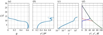
Representative example (case r2d6s2 in table 2) of solid volume fraction, shear to normal granular stress ratio, inertial number and total stress repartition depth profiles. Panel (d) shows the different components of the mixture momentum balance as a function of the depth, as derived in appendix A: the granular shear stress (—— (red)), the Reynolds shear stress (—— (blue)), the viscous shear stress (– – – (blue)), the sum of the three (—— (green)) and the slope contribution (last term of equation (A 4), – – –). The water free-surface elevation is represented in each panel for reference (——).

Considering the unidirectional character of the problem, the weighting function of the spatial averaging operator extends over the whole width and length of the periodic cell. Therefore, one obtains for each run time-averaged depth profiles of the shear and normal granular stress components:
 $\unicode[STIX]{x1D70F}^{p}(z)=\unicode[STIX]{x1D70F}_{xz}^{p}(z)$
and
 $\unicode[STIX]{x1D617}^{p}(z)=\unicode[STIX]{x1D70F}_{zz}^{p}(z)$
. Negligible stress asymmetry and compensated normal stress difference have been observed (Maurin Reference Maurin2015). Figure 2 presents typical depth profiles for a given representative simulation (run r2d6s2 in table 2). Figure 2(d) shows the different components of the streamwise mixture momentum balance, as derived in appendix A. Similarly to Revil-Baudard & Chauchat (Reference Revil-Baudard and Chauchat2013) in the sheet flow regime, the viscous stress tensor contribution is found to be negligible in turbulent bedload transport. In addition, the momentum balance is closed at each elevation, as the streamwise projection of the gravity contribution is balanced by the sum of the other terms, showing the consistency of the model formulation and stress tensor evaluation. The depth profile of the inertial number (figure 2) shows that a very important range of inertial numbers (approximately five orders of magnitude) is sampled as a function of the depth in a single simulation. This is due to the nature of bedload transport in which the granular flow evolves from quasistatic in the bed to very dynamic at the granular free surface. As the shear to normal stress ratio and the solid volume fraction vary accordingly throughout the depth (see figure 2), this allows us to obtain the granular rheology for a wide range of inertial numbers from a unique simulation. Performing simulations with variation of
 $\unicode[STIX]{x1D70C}_{p}$
,
 $d$
and
 $h$
, the water depth, the results take the form of a set of
 $\unicode[STIX]{x1D707}(I)/\unicode[STIX]{x1D719}(I)$
curves sampling the parameter space. In the present paper, each simulation will be represented by a coloured symbol, where the symbol is associated with the particle diameter
 $d$
, its colour is associated with the value of the specific density
 $\unicode[STIX]{x1D70C}_{p}/\unicode[STIX]{x1D70C}_{f}-1$
and its shading represents the Shields number (the darker the colour, the higher the Shields number) (see table 2).
3.2 Results
The influence of the interstitial fluid on the granular rheology varies between and within the different configurations investigated, and one might expect transitions between the different regimes of the
 $\unicode[STIX]{x1D707}(I)$
rheology (free-fall, turbulent, viscous). While generally of minor importance, the choice for the computation of the Stokes and
 $r$
dimensionless numbers (1.4) and (1.5) becomes crucial when approaching a transition between two regimes, as in the present analysis. In order to define accurately the different regimes and to impose that the transition from the viscous to the turbulent regime depends only on the particle Reynolds number (
 $Re_{p}=St/r$
), the limit turbulent drag coefficient
 $C_{D}^{\infty }=0.44$
should be considered, and both turbulent and viscous drag forces should be taken without the contribution from hindrance effects. However, the classical picture of the
 $\unicode[STIX]{x1D707}(I)$
rheology associates the inertial number with a time scale ratio representative of the local rearrangement process (Andreotti et al.
Reference Andreotti, Forterre and Pouliquen2013), which is affected by hindrance effects and the particle Reynolds number in the low-
 $Re_{p}$
limit of the turbulent regime (
 $Re_{p}\in [1,10^{4}]$
). Focusing on the present case (
 $St\gg 1$
and
 $r\sim 1$
so that
 $Re_{p}\gg 1$
), the
 $r$
and turbulent inertial numbers have been computed from a constant drag coefficient taking into account the local hindrance effects
 $C_{D}(z)=C_{D}^{\infty }(1-\unicode[STIX]{x1D719}(z))^{-3.1}$
, putting aside the considerations on the transition from the viscous to the turbulent regime.
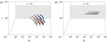
Figure 3(a) shows the parameter variation in the
 $St/r$
plane. According to the estimation of Courrech du Pont et al. (Reference Courrech du Pont, Gondret, Perrin and Rabaud2003) (
 $r_{c}\sim 6$
), all of the data belong to the turbulent regime and should show a collapse as a function of the turbulent inertial number. As can be seen from figure 3(b), this would also be the case if the
 $r$
number was evaluated without taking into account the local hindrance effect.
Positions of all of the computed granular rheology points in the (
 $St,r$
) plane, considering the drag coefficient taking into account the local hindrance effects (a) and a constant drag coefficient (b). The dashed lines represent the transition between the different regimes, with a shaded area between the expected transition from the turbulent to the free-fall regime
 $r_{c}=1$
and the one estimated by Courrech du Pont et al. (Reference Courrech du Pont, Gondret, Perrin and Rabaud2003)
 $r_{c}=6$
.

Shear to normal stress ratio
 $\unicode[STIX]{x1D707}=\unicode[STIX]{x1D70F}^{p}/\unicode[STIX]{x1D617}^{p}$
and solid volume fraction
 $\unicode[STIX]{x1D719}$
as a function of the turbulent inertial number
 $I_{turb}=\dot{\unicode[STIX]{x1D6FE}}d\sqrt{\unicode[STIX]{x1D70C}^{f}C_{D}/\unicode[STIX]{x1D617}^{p}}$
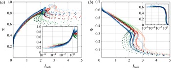
, for all of the cases presented in table 2 with variation of Shields number, specific density and particle diameter.

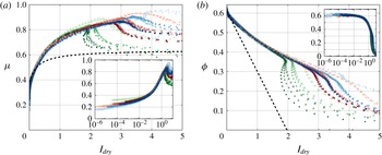
Figures 4 and 5 show the shear to normal stress ratio and the solid volume fraction as a function of the turbulent inertial number and the dry inertial number respectively. Both figures exhibit a data collapse over the range
 $I\in [10^{-2},0.1]$
. At higher inertial numbers, however, the data split apart as a function of the turbulent inertial number, while the collapse persists up to
 $I_{dry}\sim 2$
for the dry inertial number case. Therefore, the configurations sampled are better described by the dry inertial number and belong at first order to the free-fall regime, in contradiction with the predicted transition from the free-fall to the turbulent regime of Courrech du Pont et al. (Reference Courrech du Pont, Gondret, Perrin and Rabaud2003). One still notes a slight dependence on the specific density in figure 5, suggesting a second-order influence of the fluid inertial rearrangement mechanism. This absence of clear transition from the free-fall to the turbulent regime is consistent with recent global analysis of immersed granular collapse using a DNS–DEM model (Izard et al.
Reference Izard, Bonometti and Lacaze2014). Similarly to the transition from the viscous to the free-fall regime (Trulsson et al.
Reference Trulsson, Andreotti and Claudin2012), one might expect the transition region to be described by a combination of the turbulent and dry inertial numbers. In the present paper, the second-order effects are neglected for simplicity and the dry inertial number will be adopted in the following.
Shear to normal stress ratio
 $\unicode[STIX]{x1D707}=\unicode[STIX]{x1D70F}^{p}/\unicode[STIX]{x1D617}^{p}$
and solid volume fraction
 $\unicode[STIX]{x1D719}$
as a function of the dry inertial number
 $I_{dry}=\dot{\unicode[STIX]{x1D6FE}}d\sqrt{\unicode[STIX]{x1D70C}^{p}/\unicode[STIX]{x1D617}^{p}}$
for all of the cases presented in table 2 with variation of Shields number, specific density and particle diameter. The parameters of the simulation sampled and the corresponding symbols are shown in table 2. The dashed lines (– – –) represent the classical expressions of
 $\unicode[STIX]{x1D707}(I)/\unicode[STIX]{x1D719}(I)$
(1.2) and (1.3) with the parametrisation of Da Cruz et al. (Reference Da Cruz, Emam, Prochnow, Roux and Chevoir2005) and Jop et al. (Reference Jop, Forterre and Pouliquen2006):
 $\unicode[STIX]{x1D707}_{s}=0.38$
,
 $\unicode[STIX]{x1D707}_{2}=0.64$
,
 $I_{0}=0.279$
,
 $a=0.31$
.

Coming back to figure 5 and considering the semilogarithmic scale insets, the solid volume fraction curves are seen to collapse down to the lowest inertial number sampled (
 $I_{dry}\sim 10^{-5}$
). For the shear to normal stress ratio, the different curves split apart below
 $I_{dry}\sim 10^{-2}$
, following different branches depending on both the specific density and the Shields number of the run considered. No variation with the particle diameter is observed. In all cases, the stress ratio values in this region are below the expected static effective friction coefficient of the granular medium (
 $\unicode[STIX]{x1D707}_{s}\sim 0.38$
for monodisperse glass beads (Andreotti et al.
Reference Andreotti, Forterre and Pouliquen2013)). This low-inertial-number region corresponds to the lower parts of the different simulations, where a creeping regime is observed, with the solid velocity following an exponential decrease (Houssais et al.
Reference Houssais, Ortiz, Durian and Jerolmack2015; Maurin et al.
Reference Maurin, Chauchat, Chareyre and Frey2015) similar to the one observed in dry granular flows on a heap (Komatsu et al.
Reference Komatsu, Inagaki, Nakagawa and Nasuno2001; Richard et al.
Reference Richard, Valance, Métayer, Sanchez, Crassous, Louge and Delannay2008). These two features are characteristic of non-local effects (e.g. Kamrin & Koval Reference Kamrin and Koval2012; Bouzid et al.
Reference Bouzid, Trulsson, Claudin, Clément and Andreotti2013), where the granular flow is influenced by the far field, i.e. by the top granular flow in the present configuration. Despite the interest for granular media and out-of-equilibrium configurations, the quasistatic part of bedload transport does not contribute significantly to the sediment transport rate and will not be investigated further in this paper.
Towards the upper limit, the data are seen to collapse up to
 $I_{dry}\sim 2$
for both the solid volume fraction and the shear to normal stress ratio (figure 5). At higher inertial numbers, the different curves – corresponding to the different simulations – progressively exhibit a transition to a different behaviour characterised by a decrease of the shear to normal stress ratio, and a slope break on the solid volume fraction versus inertial number curves.
The observed decrease in the shear to normal stress ratio as a function of the inertial number is characteristic of the transition from dense to dilute granular behaviour (Forterre & Pouliquen Reference Forterre and Pouliquen2008). In the present results, the position of the transition in terms of inertial number is particularly high (
 $I\sim 2{-}3$
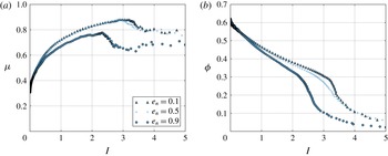
) and depends on the configurations sampled (figure 5). At such a high inertial number, the restitution coefficient is seen to have a non-negligible effect on the rheological curves (see figure 6). Focusing on the classical dry granular flow literature (e.g. Da Cruz et al.
Reference Da Cruz, Emam, Prochnow, Roux and Chevoir2005; Jop et al.
Reference Jop, Forterre and Pouliquen2006; Forterre & Pouliquen Reference Forterre and Pouliquen2008; Jop Reference Jop2015), the
 $\unicode[STIX]{x1D707}(I)$
approach is considered to break down above
 $I_{dry}\sim 0.5$
for glass beads, when collisional mechanisms comes into play (Da Cruz et al.
Reference Da Cruz, Chevoir, Roux, Iordanoff, Dalmaz, Lubrecht, Dowson and Priest2004; Lois, Lemaître & Carlson Reference Lois, Lemaître and Carlson2006; Forterre & Pouliquen Reference Forterre and Pouliquen2008). Therefore, it is unable to explain both the observed variation of the transition position at constant restitution coefficient and the collapse observed in regions where collisional mechanisms contribute non-negligibly to the rheology.
Effect of the restitution coefficient on the shear to normal stress ratio
 $\unicode[STIX]{x1D707}=\unicode[STIX]{x1D70F}^{p}/\unicode[STIX]{x1D617}^{p}$
and solid volume fraction
 $\unicode[STIX]{x1D719}$
as a function of the dry inertial number
 $I_{dry}=\dot{\unicode[STIX]{x1D6FE}}d\sqrt{\unicode[STIX]{x1D70C}^{p}/\unicode[STIX]{x1D617}^{p}}$
for a representative case (case r2d6s2 in table 2).

Recently, similar persistence of dense granular flow behaviour at high inertial numbers has been observed in inclined plane configurations. Holyoake & McElwaine (Reference Holyoake and Mcelwaine2012) observed experimentally dense granular flows up to inertial numbers
 $I_{dry}\sim 2$
in steady non-uniform dry granular flows of sand in a steep channel with lateral walls and a bumpy base. Moreover, analysing granular roll wave instabilities using the DEM, Börzsönyi, Ecke & McElwaine (Reference Börzsönyi, Ecke and Mcelwaine2009) computed the local granular rheology and obtained a collapse of their rheological data up to
 $I_{dry}\sim 1$
. In these two configurations as well as in the present study, the complexity of the granular flow considered can lead to differences with respect to the simple shear picture. In particular, the local analysis of spatially non-homogeneous granular flows made in the present paper and in Börzsönyi et al. (Reference Börzsönyi, Ecke and Mcelwaine2009) might lead to secondary gradient effects that are not taken into account in the
 $\unicode[STIX]{x1D707}(I)$
rheology. Therefore, the local character of the analysis and/or the specificity of the configuration seem to affect the persistence of a dense granular flow at high inertial numbers.
As a consequence of the high-inertial-number collapse, the classical
 $\unicode[STIX]{x1D707}(I)/\unicode[STIX]{x1D719}(I)$
expressions (1.2) and (1.3) and parametrisation do not fit the present results well at high inertial numbers (see the fit of Jop et al. (Reference Jop, Forterre and Pouliquen2006) in figure 5). Indeed, the collisional contribution becomes important in this region and one might need to extend the
 $\unicode[STIX]{x1D707}(I)/\unicode[STIX]{x1D719}(I)$
relationships as done by Holyoake & McElwaine (Reference Holyoake and Mcelwaine2012) for the inclined plane configuration.
The results have evidenced the ability of the
 $\unicode[STIX]{x1D707}(I)$
framework to describe the granular flow rheology in bedload transport in the dense granular flow region. They have shown that the interstitial fluid does not influence the dense granular rheology importantly and that the fluid flow acts mainly as an external forcing in turbulent bedload transport. In addition, the analysis has underlined the variety and the complexity of the granular behaviours observed in bedload transport, which challenge the existing formulation of the
 $\unicode[STIX]{x1D707}(I)$
rheology.
4 Granular rheology in bedload transport
The rest of this paper focuses on the analysis of turbulent bedload transport, considering realistic conditions typical of gravel-bed rivers. Therefore, the specific density is taken as
 $\unicode[STIX]{x1D70C}^{p}/\unicode[STIX]{x1D70C}^{f}-1=1.5$
and additional DEM simulations are performed at Shields numbers down to the onset of motion. The analysis of the DEM results allows us to propose a
 $\unicode[STIX]{x1D707}(I)$
-based granular rheology for turbulent bedload transport. The relevance of the proposed granular rheology is further tested using the Eulerian–Eulerian model presented in § 2.
4.1 Parametrisation of the
 $\unicode[STIX]{x1D707}(I)$
rheology

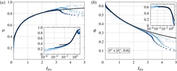
Figure 7 shows the granular shear to normal stress ratio and the solid volume fraction as a function of the inertial number, for simulations with Shields numbers from
 $\unicode[STIX]{x1D703}^{\ast }=0.04$
to
 $\unicode[STIX]{x1D703}^{\ast }=0.6$
and for particle diameters
 $d\in \{3;6;12\}$
mm. In these new configurations closer to realistic bedload transport, most of the data are seen to collapse for both the solid volume fraction and the granular stress ratio up to high inertial numbers. Above
 $I\sim 3$
and under
 $I\sim 10^{-2}$
, the curves split apart similarly to the general case. No dependence upon the particle diameter is observed over the whole range of inertial numbers, pointing out the negligible effect of the
 $Re_{p}$
and
 $St$
numbers in the problem. The lowest-Shields-number cases (lightest points) exhibit some specific behaviour with oscillations, lower shear to normal stress ratio and solid volume fraction at given inertial numbers. These cases correspond to the sharpest transitions between a quasistatic granular bed and a few particles in motion on top of it. Therefore, in these configurations the continuous assumption is not strictly valid and the limits of the rheological description are reached.
Shear to normal stress ratio and solid volume fraction as a function of the dry inertial number, for realistic bedload transport simulations with specific density
 $\unicode[STIX]{x1D70C}^{p}/\unicode[STIX]{x1D70C}^{f}-1=1.5$
, Shields number from incipient motion to
 $0.7$
and particle diameter of
 $d=3$
mm,
 $d=6$
mm and
 $d=12$
mm. The black lines represent the best fit obtained with equations (1.2) and (4.1) (
 $\unicode[STIX]{x1D707}_{1}=0.38$
,
 $\unicode[STIX]{x1D707}_{2}=0.64$
,
 $I_{0}=0.279$
,
 $\unicode[STIX]{x1D719}^{max}=0.61$
and
 $b=0.31$
). The symbol colours are functions of the simulation Shields number: the darker the colour, the higher the Shields number.

Overriding these limitations close to the critical Shields number and assuming that the high-inertial-number granular behaviour is not dominant in bedload transport, the
 $\unicode[STIX]{x1D707}(I)$
constitutive laws are pragmatically best-fitted on the Eulerian–Lagrangian simulation results over the range of inertial numbers
 $I_{dry}\in [10^{-2},3]$
. The classical solid volume fraction expression (1.3) predicts negative values at high inertial numbers and is unable to describe the present results. Consequently, the expression is modified and is chosen following Aussillous et al. (Reference Aussillous, Chauchat, Pailha, Médale and Guazzelli2013) and Revil-Baudard & Chauchat (Reference Revil-Baudard and Chauchat2013) as
 $$\begin{eqnarray}\displaystyle \unicode[STIX]{x1D719}(I)=\frac{\unicode[STIX]{x1D719}^{max}}{1+bI}. & & \displaystyle\end{eqnarray}$$
The best fits of equations (1.2) and (4.1) on the data give the following parameters:
 $b=0.31$
,
 $\unicode[STIX]{x1D707}_{s}=0.35$
,
 $\unicode[STIX]{x1D707}_{2}=0.97$
and
 $I_{0}=0.69$
, with
 $\unicode[STIX]{x1D719}^{max}$
imposed to take the value measured in the Eulerian–Lagrangian simulations:
 $\unicode[STIX]{x1D719}^{max}=0.61$
. Developing the solid volume fraction expression around
 $I=0$
, the value of
 $b$
obtained is consistent with both the parametrisation of Da Cruz et al. (Reference Da Cruz, Emam, Prochnow, Roux and Chevoir2005) in the dry regime and the one of Boyer et al. (Reference Boyer, Guazzelli and Pouliquen2011) and Trulsson et al. (Reference Trulsson, Andreotti and Claudin2012) in the viscous regime. The values of
 $\unicode[STIX]{x1D707}_{2}$
and
 $I_{0}$
are logically higher than in the original
 $\unicode[STIX]{x1D707}(I)$
rheology, as no real saturation of the stress ratio is observed in our data. The best fits describe very well the results obtained within the collapsing range of
 $I_{dry}$
, as can be seen in figure 7. Outside this interval, they do not reproduce the non-local effects at low inertial numbers (
 $I_{dry}<10^{-2}$
) and the drop in both the shear to normal stress ratio and the solid volume fraction for
 $I_{dry}>3$
.
Assuming the dense granular behaviour to be dominant, the two relationships (1.2)–(4.1) together with the values determined from the best fits are proposed as a
 $\unicode[STIX]{x1D707}(I)$
-based granular rheology for turbulent bedload transport.
4.2 Eulerian–Eulerian simulations
In order to evaluate the relevance of the proposed granular rheology it has been implemented in the Eulerian–Eulerian model presented in § 2. Simulations have been performed using exactly the same parameters for both the Eulerian–Lagrangian and the Eulerian–Eulerian models (
 $\unicode[STIX]{x1D70C}_{p}/\unicode[STIX]{x1D70C}_{f}-1=1.5$
;
 $d=6$
mm,
 $\unicode[STIX]{x1D6FC}=0.05$
,
 $h$
). The particle diameter has been varied (
 $d\in 3,6,12$
mm) but does not influence the results, so that only the case
 $d=6$
mm is presented for clarity.
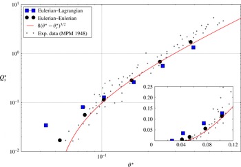
Dimensionless sediment transport rate as a function of the Shields number for two-phase continuous simulations (Eulerian–Eulerian) and coupled fluid–discrete-element simulations (Eulerian–Lagrangian), with realistic parameters for turbulent bedload transport:
 $\unicode[STIX]{x1D70C}^{p}/\unicode[STIX]{x1D70C}^{f}-1=1.5$
and
 $d=6$
mm. The black crosses and the red line represent the data and the fit of Meyer-Peter & Müller (Reference Meyer-Peter and Müller1948) respectively.

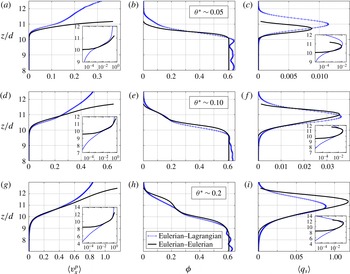
Solid depth profile comparison between the two-phase continuous model (Euler–Euler) and the coupled fluid–discrete-element model (Euler–Lagrange) for three different Shields numbers
 $\unicode[STIX]{x1D703}^{\ast }$
with
 $d=6$
mm and
 $\unicode[STIX]{x1D70C}^{p}/\unicode[STIX]{x1D70C}^{f}-1=1.5$
. The solid velocity
 $\langle v_{x}^{p}\rangle ^{s}$
and transport rate density
 $\langle q_{s}\rangle ^{s}$
are expressed in
 $\text{m}~\text{s}^{-1}$
while the solid volume fraction is dimensionless. The fluid mechanics convention is used.

Figure 8 presents the dimensionless sediment transport rate versus the Shields number for the Eulerian–Eulerian model, the Eulerian–Lagrangian model and the experimental data and empirical law of Meyer-Peter & Müller (Reference Meyer-Peter and Müller1948). A good agreement with the experimental data is obtained using both models. The proposed granular rheology enables the Eulerian–Eulerian model to accurately reproduce the critical Shields number (
 $\unicode[STIX]{x1D703}_{c}^{\ast }\sim 0.04$
) and the global trend over a wide range of Shields numbers (
 $\unicode[STIX]{x1D703}^{\ast }\in [\unicode[STIX]{x1D703}_{c}^{\ast },0.7]$
). Quite surprisingly, the Eulerian–Eulerian model better predicts the smooth transition around the critical Shields number, in a region where the continuous assumption breaks down. Conversely, at high Shields numbers the increased importance of the dilute region, which is not well described by the proposed rheology (§ 4.1), induces a slight discrepancy between the Eulerian–Eulerian and Eulerian–Lagrangian models.
To go further in the analysis, the comparison is extended to the granular depth profiles by decomposing the sediment transport rate into the integral of the sediment transport rate density
 $\langle q_{s}\rangle (z)=\langle v_{x}\rangle ^{s}(z)\unicode[STIX]{x1D719}(z)$
(Bagnold Reference Bagnold1956):
 $$\begin{eqnarray}\displaystyle Q_{s}=\int _{0}^{\infty }\langle q_{s}\rangle (z)\,\text{d}z=\int _{0}^{\infty }\langle v_{x}\rangle ^{s}(z)\,\unicode[STIX]{x1D719}(z)\,\text{d}z. & & \displaystyle\end{eqnarray}$$
Figure 9 shows the comparison of the solid volume fraction, the solid velocity and the transport rate density profiles obtained with the Eulerian–Eulerian and Eulerian–Lagrangian models for three different Shields numbers
 $\unicode[STIX]{x1D703}^{\ast }=\{0.05;0.1;0.2\}$
. The Eulerian–Eulerian model reproduces accurately the granular depth profiles obtained with the Eulerian–Lagrangian model for solid volume fractions approximately higher than 0.3 (
 $\unicode[STIX]{x1D719}\gtrsim 0.3$
). This value roughly corresponds to the domain for which the proposed granular rheology describes the Eulerian–Lagrangian results very well (see figure 7). Only the lower quasistatic velocity profile – negligible in terms of sediment transport rate – is not reproduced, as non-local effects have not been taken into account in the granular rheology. In the dilute region (
 $\unicode[STIX]{x1D719}\lesssim 0.3$
), the particle velocity is overestimated by the Eulerian–Eulerian model for the three different Shields numbers, showing an increasing discrepancy towards the lower solid volume fraction region. This is associated with an underestimation of the solid volume fraction close to incipient motion and an overestimation at high Shield numbers. These behaviours point out both the ill-posedness of the
 $\unicode[STIX]{x1D707}(I)$
rheology as the solid volume fraction goes to zero and the inability of the proposed rheology to describe the dilute region accurately. Despite these limitations, the good lower boundary condition given by the accurate description of the dense granular flow constrains the dilute behaviour and enables a good description of the sediment transport rate over a wide range of Shields numbers with the Eulerian–Eulerian model.
The present results show that a
 $\unicode[STIX]{x1D707}(I)$
rheology is able to reproduce the main features of turbulent bedload transport in terms of sediment transport rate and dense granular depth profiles, in steady uniform configurations. Considering the much lower computational cost of Eulerian–Eulerian simulations compared with Eulerian–Lagrangian ones, it will allow an important step to be made in the upscaling process towards applications. In this perspective, the fluid phase description might have to be upgraded, using a two-equation turbulence model such as
 $k$
–
 $\unicode[STIX]{x1D716}$
or
 $k$
–
 $\unicode[STIX]{x1D714}$
(Hsu et al.
Reference Hsu, Jenkins and Liu2004; Amoudry Reference Amoudry2014; Lee, Low & Chiew Reference Lee, Low and Chiew2016) or eddy resolving simulations.
5 Summary and conclusion
The granular rheology in idealised turbulent bedload transport has been studied using a coupled fluid–discrete-element model. Computing the granular stress tensor locally as a function of the depth and performing simulations for various Shields numbers, specific densities and particle diameters, the data have been shown to collapse over an important range of inertial numbers, demonstrating the relevance of the
 $\unicode[STIX]{x1D707}(I)$
rheology for turbulent bedload transport description. No clear transition from the free-fall to the turbulent regime of the
 $\unicode[STIX]{x1D707}(I)$
rheology has been observed, supporting recent numerical observations and suggesting that the interstitial fluid does not importantly influence the granular rheology in turbulent bedload transport. In addition, consistently with recent literature, the data have been observed to collapse in terms of both the solid volume fraction and the shear to normal stress ratio, up to inertial numbers as high as
 $I\sim 2$
. The persistence of a dense granular flow behaviour at such a high inertial number together with the observed progressive transition from dense to dilute behaviour challenges the classical conceptions and parametrisations of the
 $\unicode[STIX]{x1D707}(I)$
rheology, and opens interesting perspectives for a better understanding of granular media rheology at high inertial numbers. Beyond these observations, a
 $\unicode[STIX]{x1D707}(I)$
-based granular rheology has been fitted to the present Eulerian–Lagrangian bedload transport simulations. The proposed rheology has been successfully tested using a Eulerian–Eulerian model. It has been shown to accurately reproduce the dense granular depth profiles and the classical experimental results in terms of sediment transport rate from the onset of motion up to a Shields number of
 $\unicode[STIX]{x1D703}^{\ast }\sim 0.7$
.
Further work is needed to better understand the high-inertial-number behaviour and extend the granular rheology to the description of the dilute region. At this stage it is not clear whether the
 $\unicode[STIX]{x1D707}(I)$
rheology could be extended to handle this regime transition. Besides, the proposed rheology can already be used in three-dimensional Eulerian–Eulerian numerical models and represents a step in the upscaling process from particle-scale simulations towards full-scale problem modelling.
Acknowledgements
We are grateful to the three anonymous reviewers for relevant and constructive questions, and to A. Dudill for English corrections. R.M. would like to thank T. Faug for fruitful discussions. This research was supported by Irstea (formerly Cemagref), the labex OSUG@2020 and the French Institut National des Sciences de l’Univers programs EC2CO-BIOHEFECT and EC2CO-LEFE MODSED.
Appendix A. Momentum balance derivation
In order to validate the stress tensor profile computed, the momentum balance is analysed in the framework of the continuous two-phase equations (Jackson Reference Jackson2000). In the present appendix, the equations are derived and integrated to show the exact terms computed in the body of the paper. Using the steady and uniform character of the problem considered, the momentum balances for both the fluid and the granular phases read along the streamwise direction (Jackson Reference Jackson2000)
 $$\begin{eqnarray}\displaystyle & \displaystyle 0=\frac{\unicode[STIX]{x2202}\unicode[STIX]{x1D61A}_{xz}^{f}}{\unicode[STIX]{x2202}z}+\frac{\unicode[STIX]{x2202}\unicode[STIX]{x1D619}_{xz}^{f}}{\unicode[STIX]{x2202}z}+\unicode[STIX]{x1D70C}^{f}(1-\unicode[STIX]{x1D719})g\sin \unicode[STIX]{x1D6FC}-n\langle {f_{f}^{p}}_{x}\rangle ^{p}, & \displaystyle\end{eqnarray}$$
 $$\begin{eqnarray}\displaystyle & \displaystyle 0=\frac{\unicode[STIX]{x2202}\unicode[STIX]{x1D70F}_{xz}^{p}}{\unicode[STIX]{x2202}z}+\unicode[STIX]{x1D70C}^{p}\unicode[STIX]{x1D719}g\sin \unicode[STIX]{x1D6FC}+n\langle {f_{f}^{p}}_{x}\rangle ^{p}. & \displaystyle\end{eqnarray}$$
Combining these two equations together, the mixture momentum balance can be written as
 $$\begin{eqnarray}\displaystyle 0=\frac{\unicode[STIX]{x2202}\unicode[STIX]{x1D61A}_{xz}^{f}}{\unicode[STIX]{x2202}z}+\frac{\unicode[STIX]{x2202}\unicode[STIX]{x1D619}_{xz}^{f}}{\unicode[STIX]{x2202}z}+\frac{\unicode[STIX]{x2202}\unicode[STIX]{x1D70F}_{xz}^{p}}{\unicode[STIX]{x2202}z}+(\unicode[STIX]{x1D70C}^{p}\unicode[STIX]{x1D719}+(1-\unicode[STIX]{x1D719})\unicode[STIX]{x1D70C}^{f})g\sin \unicode[STIX]{x1D6FC}. & & \displaystyle\end{eqnarray}$$
In order to study the stress repartition, the equation is integrated between a given position
 $z$
in
 $h>z>0$
and the water free-surface elevation
 $h$
, where the viscous, turbulent and particle shear stresses vanish:
 $\unicode[STIX]{x1D61A}_{xz}^{\,f}(h)=\unicode[STIX]{x1D619}_{xz}^{\,f}(h)=\unicode[STIX]{x1D70F}_{xz}^{p}(h)=0$
. It leads to the following formulation:
 $$\begin{eqnarray}\displaystyle 0=-\unicode[STIX]{x1D61A}_{xz}^{\,f}(z)-\unicode[STIX]{x1D619}_{xz}^{\,f}(z)-\unicode[STIX]{x1D70F}_{xz}^{p}(z)+g\sin \unicode[STIX]{x1D6FC}\left[\unicode[STIX]{x1D70C}^{f}(h-z)+(\unicode[STIX]{x1D70C}^{p}-\unicode[STIX]{x1D70C}^{f})\int _{z}^{h}\unicode[STIX]{x1D719}\,\text{d}z\right]. & & \displaystyle\end{eqnarray}$$
From one simulation, it is possible to evaluate all of the terms of the equation at each given elevation. Provided that the stress tensor formulation is appropriate and the system is at equilibrium, the equality should be satisfied.