


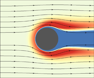



1. Introduction
Studies on electrophoresis of colloids are important for characterization, separation and manipulation of colloids and macromolecules pertaining to microfluidic and nanofluidic devices (Pysher & Hayes Reference Pysher and Hayes2007; Surugau & Urban Reference Surugau and Urban2009; Sonker et al. Reference Sonker, Kim, Egatz-Gomez and Ros2019; Hettiarachchi et al. Reference Hettiarachchi, Cha, Ouyang, Mudugamuwa, An, Kijanka, Kashaninejad, Nguyen and Zhang2023). The electrophoresis of a charged colloid subjected to an externally imposed electric field is a phenomenon that arises due to the interaction of the electrostatic Coulomb force and the polarization and relaxation of the double layer created by the particles. It is established that a linear dependence of the electrophoresis with the imposed electric field occurs when the distortion of the double layer leading to double-layer relaxation and polarization is negligible (O'Brien & White Reference O'Brien and White1978; Schnitzer & Yariv Reference Schnitzer and Yariv2012a). Several theories on electrophoresis have been developed under a weak electric field, i.e. the potential drop created by the applied field across a particle is smaller than the the thermal potential ( $\phi _0$) and the
 $\zeta$ potential of the order of the thermal potential
 $\phi _0$ (Von Smoluchowski Reference Von Smoluchowski1921; O'Brien & White Reference O'Brien and White1978; Ohshima, Healy & White Reference Ohshima, Healy and White1983; Stout & Khair Reference Stout and Khair2017). These theories are developed by considering an electric double layer (EDL) or Debye layer of mobile space charge density screening the surface charge which forms around the particle and extends to the outer electrically neutral fluid. The double-layer polarization and relaxation arising due to the deformation of the EDL is addressed. However, this form of EDL modifies in the presence of a strong imposed electric field, which draws a large number of ions in the vicinity of the particle and, hence, produces an enhanced surface conduction. At a large imposed electric field a thin layer of diffuse charge clouds develops at the outer surface of the primary EDL to balance the tangential ion flux with the transverse ion flux around the particle (Dukhin Reference Dukhin1991; Barany, Madai & Shilov Reference Barany, Madai and Shilov2004). In this case, the tangential electric field on the space charge of the diffuse layer creates an additional electro-osmotic flow (Dukhin Reference Dukhin1991). In addition, at a sufficiently high electric field the double-layer relaxation may cause the double layer to be stripped off the particle (Williams & Williams Reference Williams and Williams1978). At a stronger electric field during the double-layer relaxation time, the particle travels the distance beyond the extension of the double layer. In this case, the mobility becomes independent of the bulk ionic concentration.
The classical Smoluchowski theory, which is based on the absence of Debye layer polarization, predicts that the mobility of rigid colloids for a Debye length much smaller than the particle size (thin Debye layer) is electric-field-independent and can be treated as an intrinsic property of the colloid. This theory is valid under a weak electric field. Deviation from this Smoluchowski theory to a large extent occurs at a strong electric field due to the formation of a secondary diffuse layer of counterions outside the primary EDL screening the surface charge. Dukhin (Reference Dukhin1991) proposed a velocity correction to the Smoluchowski mobility which accounts for the non-uniformity of the  $\zeta$ potential at a larger electric field and significant ionic currents through the diffuse portion of the double layer. The electrophoresis velocity may become higher than the velocity predicted by the Smoluchowski limit at a sufficiently strong electric field. An asymptotic analysis for the nonlinear electrophoretic motion of highly charged particles in the thin Debye layer limit is developed by Schnitzer & Yariv (Reference Schnitzer and Yariv2012a).
The nonlinear effect of the electrokinetic phenomena can be categorized by two dimensionless parameters. The Dukhin number ( $Du$) determines the ratio between particle surface conductivity and bulk conductivity (Dukhin, Dukhin & Mishchuk Reference Dukhin, Dukhin and Mishchuk1988; Mishchuk & Dukhin Reference Mishchuk and Dukhin1989, Reference Mishchuk and Dukhin2002) and the Péclet number describes the balance between convective and diffusive processes near the particle surface. By considering a low but non-zero Dukhin number, Schnitzer & Yariv (Reference Schnitzer and Yariv2014) derived an analytical expression for the velocity valid for small ions (low Péclet number), the nonlinear part of which is proportional to electric field cubed. The Smoluchowski velocity recovers for a zero
 $Du$ (which corresponds to insignificant surface conduction). This growth in mobility with an electric field under
 $Du<1$ decays and becomes proportional to 3/2 power of the imposed field for a sufficiently large Péclet number (Dukhin Reference Dukhin1991; Schnitzer & Yariv Reference Schnitzer and Yariv2014; Cobos & Khair Reference Cobos and Khair2023). The experimental validations of these theories for mobility are provided by several authors (Rouhi Youssefi & Diez Reference Rouhi Youssefi and Diez2016; Bentor et al. Reference Bentor, Dort, Chitrao, Zhang and Xuan2023; Lomeli-Martin et al. Reference Lomeli-Martin, Ernst, Cardenas-Benitez, Cobos, Khair and Lapizco-Encinas2023) for either a very small or a very large Péclet number for which
 $Du<1$. These studies show an agreement of the experimentally measured mobility with the theoretical prediction. However, due to the complexity of the problem, no theory is available for intermediate Péclet number for which
 $Du$ is
 $O(1)$. Tottori et al. (Reference Tottori, Misiunas, Keyser and Bonthuis2019) found that the theory developed by Schnitzer & Yariv (Reference Schnitzer and Yariv2014) based on the assumption of small Dukhin and Péclet numbers shows a reasonable agreement with the experimental data. They have shown that highly charged non-conducting particles exhibit nonlinear electrophoretic velocity at high electric fields. Lomeli-Martin et al. (Reference Lomeli-Martin, Ernst, Cardenas-Benitez, Cobos, Khair and Lapizco-Encinas2023) have shown experimentally that both particle size and charge characterize nonlinear electrophoresis.
Most of the theoretical and experimental studies on developing the theory of electrophoresis are focused on monovalent electrolytes with moderate range of surface charge density. These studies are based on the mean-field consideration, in which the contribution of the ions in the medium is accounted for through the force potential. However, such formulation cannot explain the overscreening and charge density oscillation as found in an electrolyte medium involving multivalent counterions.
The experimental study of Diehl & Levin (Reference Diehl and Levin2006) and Kubíčková et al. (Reference Kubíčková, Křížek, Coufal, Vazdar, Wernersson, Heyda and Jungwirth2012) on capillary electrophoresis shows a mobility reversal in multivalent electrolytes beyond a critical ionic strength of the La(Ac) $_3$ electrolyte, which arises due to the overcompensation of the particle charge by the solvent electrolyte. A region of charge inversion arises at a short distance from the particle surface. It was shown that the results based on the linearized Poisson–Boltzmann model overestimate the Monte Carlo simulations for monovalent electrolytes and becomes invalid for multivalent salts. Several experimental studies show that the magnitude of the mobility determined through the theoretical analysis based on the point-charge Poisson–Boltzmann model is significantly larger than the experimentally measured data (Martın-Molina et al. Reference Martın-Molina, Quesada-Pérez, Galisteo-González and Hidalgo-Álvarez2003; Quesada-Pérez et al. Reference Quesada-Pérez, González-Tovar, Martín-Molina, Lozada-Cassou and Hidalgo-Álvarez2005; Nishiya, Sugimoto & Kobayashi Reference Nishiya, Sugimoto and Kobayashi2016). In these studies, the limitations of the mean-field-based approach in analysing the electrophoresis involving multivalent counterions are elaborated. Semenov et al. (Reference Semenov, Raafatnia, Sega, Lobaskin, Holm and Kremer2013) and references therein demonstrate the occurrence of mobility reversal as the concentration of trivalent counterions is increased. Diehl & Levin (Reference Diehl and Levin2006) have shown that below a critical surface charge density the mobility reversal may not occur even for a large trivalent electrolyte concentration.
The standard continuum models based on the Nernst–Planck–Poisson (PNP) model equations predict a repulsion of like-charged ions and neglect the correlations between ions. These models cannot predict the overscreening and oscillation in charge density within the Debye layer, which is attributed to Coulomb short-range electrostatic correlations. Based on a molecular dynamics simulation, Raafatnia et al. (Reference Raafatnia, Hickey, Sega and Holm2014) concluded that the standard mean-field-based model can exhibit mobility reversal in a multivalent salt, provided the ion correlations are incorporated.
Earlier, the ionic correlations were accounted for through a Monte Carlo simulation by adopting the primitive model in which the ions behave like charged dielectric hard spheres embedded in a dielectric electrolyte medium (Das et al. Reference Das, Bratko, Bhuiyan and Outhwaite1997). Santangelo (Reference Santangelo2006) and subsequently Hatlo & Lue (Reference Hatlo and Lue2010) proposed approaches to determine the counterion distribution near a charged surface by decomposing the Coulomb interactions into weak coupling and short coupling components. The weak coupling of ions is governed by the mean-field-based approach, whereas the short-range interactions become important in the strong coupling regime, which is designated by a higher value of the coupling parameter  $\varGamma$, measuring the ratio between the Bjerrum length and the Gouy–Chapman length. Based on this approach of splitting the ion–ion interactions regime, Bazant, Storey & Kornyshev (Reference Bazant, Storey and Kornyshev2011) accounted for the many-body ion–ion correlations under the continuum hypothesis by deriving a modified Gauss law. In this model (Bazant et al. Reference Bazant, Storey and Kornyshev2011; Storey & Bazant Reference Storey and Bazant2012; de Souza et al. Reference de Souza, Goodwin, McEldrew, Kornyshev and Bazant2020) the non-local short-range interactions arising due to ion–ion correlations are incorporated in the energy density functional, which leads to the fourth-order Poisson–Fermi equation for electric field. This formulation involves a parameter, the correlation length, signifying the importance of the ionic correlation. The oscillations in the ion density occur at the scale of the correlation length. The correlation length is bounded below by the counterion size and is of the order of the Bjerrum length, the distance at which two unit charges interact with thermal energy, for a lower charge density limit. de Souza et al. (Reference de Souza, Goodwin, McEldrew, Kornyshev and Bazant2020) proposed that for a highly charged surface, in which ion–ion repulsion dominates, the correlation length scales as the size of a correlation hole and provided a power-law expression for the correlation length verifying the Monte Carlo simulation. This modification of the continuum model to incorporate electrostatic correlation has been adopted by several authors and demonstrated the surface charge overscreening and charge density oscillation and established a close agreement with molecular dynamics simulation and/or Monte Carlo simulation (Storey & Bazant Reference Storey and Bazant2012; Raafatnia et al. Reference Raafatnia, Hickey, Sega and Holm2014; Stout & Khair Reference Stout and Khair2014; Celebi, Cetin & Beskok Reference Celebi, Cetin and Beskok2019; de Souza et al. Reference de Souza, Goodwin, McEldrew, Kornyshev and Bazant2020). Stout & Khair (Reference Stout and Khair2014) adopted the continuum approach as described by Bazant et al. (Reference Bazant, Storey and Kornyshev2011) and demonstrated electrophoresis mobility reversal in a multivalent electrolyte.
Consideration of ions as finite-sized charged spheres suspended in an aqueous medium leads to the manifestation of ion steric repulsion and viscosity variation with the local volume fraction of ions. In all those studies described above, the hydrodynamic steric interactions of finite-sized ions are incorporated by introducing the excess electrochemical potential based on the Bikerman model (Bikerman Reference Bikerman1942). This Bikerman model to account for steric repulsion is easy to implement; however, this model for analysing steric interaction is inefficient and does not produce counterion saturation when the local volume fraction of the ion is below  $O(1)$ (López-García, Horno & Grosse Reference López-García, Horno and Grosse2014). Contrary to the Bikerman model, the excluded volume effect based on the Carnahan–Starling model (Carnahan & Starling Reference Carnahan and Starling1969) can produce saturation in counterions for a moderate range of local volume fraction,
 $\nu \sim O(10^{-3})$. The Carnahan–Starling model can be extended to consider interactions of unequal-sized ions by adopting the Boublik–Mansoori–Carnahan–Starling–Leland (BMCSL) equation of state (Boublík Reference Boublík1970; Mansoori et al. Reference Mansoori, Carnahan, Starling and Leland1971). Several studies based on molecular dynamics simulation show that the viscosity of the medium near a charged surface is enhanced due to larger accumulation of ions. The effective viscosity of the suspension medium can be obtained by the Batchelor–Green equation based on two-particle hydrodynamic interactions, which has been adopted by López-García, Horno & Grosse (Reference López-García, Horno and Grosse2019) in the context of electrokinetic transport involving finite-sized ions.
A stronger electric field draws an excess amount of ions in the Debye layer of a particle. This creates an ion crowding effect even in a dilute situation. Bazant et al. (Reference Bazant, Storey and Kornyshev2011) demonstrated that increasing the voltage attenuates the surface charge overscreening by extending the condensed layer of counterions towards the bulk, which in turn draws excess co-ions in the Debye layer. The saturation in counterions in the Debye layer resulting from the steric repulsion of ions can enable the mean-field-based model to predict the experimentally observed camel-shape curve between the differential capacitance of the Debye layer and applied voltage (Kornyshev Reference Kornyshev2007). Thus, the crowding effect becomes significant at a larger voltage even for a dilute bulk solution. This counterion saturation in the EDL attenuates the large increment in velocity with the applied electric field.
In this paper we consider the nonlinear electrophoresis of a rigid colloid at a stronger imposed electric field in a monovalent as well as a valence asymmetric electrolyte. We devise a continuum model, which incorporates the finite-ion-size effects and the ion–ion electrostatic correlations, to analyse the nonlinear electrophoresis. One of the objectives of this study is to analyse the impact of the hydrodynamic ion steric interactions and many-body interactions in ion–ion correlations on nonlinear electrophoresis at a high applied electric field. In contrast to molecular dynamics simulations and other non-local approaches, the continuum models are cost-effective and easy to implement. The fourth-order modified Poisson equation for electric field is considered to capture non-equilibrium phenomena arising due to the electrostatic correlations of ions. This equation is coupled with the ion transport equation which incorporates the ion steric interactions governed by the BMCSL equation of state. The motion of the ionized fluid is governed by the Navier–Stokes equations. As the ions are considered to be dielectric charged spheres of finite size, the viscosity of the medium becomes dependent on the local ionic volume fraction and it is modelled through the Batchelor–Green two-particle hydrodynamics model (Batchelor & Green Reference Batchelor and Green1972). Modification of the viscosity alters the diffusivity of the ions. We have solved the governing equations by adopting a control-volume-based approach. We have validated our numerical model by comparing it with existing experimental results and several previous theoretical analyses under specific limiting conditions. Our numerical model is supplemented by a simplified model developed under a weak imposed field consideration. We have derived an expression for mobility for the modified model under the Smoluchowski limit valid for a weak applied field.
2. Mathematical model
We consider the electrophoresis of a non-polarizable charged spherical particle of radius  $a$ and surface charge density
 $\sigma ^*$ immersed in an electrolyte solution of dielectric permittivity
 $\varepsilon _e$ moving with electrophoretic velocity
 $U^{*}_{E}$ in response to an applied electric field
 $E_0$. Spherical polar coordinates (
 $r^*,\theta,\psi$) are adopted with the origin fixed at the centre of the particle and the
 $z$ axis (
 $\theta$ = 0) is along the imposed applied electric field
 $E_0$ (figure 1). This problem can be treated as axially symmetric with the
 $z$ axis as the axis of symmetry.
Schematic of a rigid colloid with surface charge density  $\sigma ^{*}$ suspended in an electrolyte where the sizes of the cations and anions are given by
 $2\tau _+$ and
 $2\tau _-$, respectively, moving under the influence of applied electric field
 $\boldsymbol {E}_{0}$.

We consider  $a$ as the length scale, the thermal potential
 $\phi _0=k_BT/e$ is the electric potential scale, surface charge density is scaled by
 $\epsilon _{e}\phi _0/a$,
 $U_0=\epsilon _{e} \phi _{0}^2/\mu _w a$ is the velocity scale,
 $\tau =a/U_0$ is the time scale and pressure is scaled by
 $p_0$ (
 $=U_0{\mu _w}/a$). The scale for the ionic concentration is the bulk ionic strength
 $I_{\infty }=\tfrac {1}{2}\sum _{i}z_{i}^2n_i^{\infty }$, where
 ${n_{i}^{\infty }}$ is the bulk number concentration of the
 $i{{\rm th}}$ ionic species with valence
 $z_{i}$, which can be determined from the bulk number concentration (
 $n^{\infty }$). Here
 $e$ is the elementary charge,
 $k_B$ is the Boltzmann constant,
 $T$ is the absolute temperature and
 $\mu _w$ is the viscosity of the medium in infinite dilution. Here,
 $\rho _e=\sum _{i=1}^{n}{z_{i}n_{i}}$ is the charge density with
 $n_i$ (
 $i = 1,2$) being the number concentration of the
 $i{{\rm th}}$ ionic species with valence
 $z_i$. Here
 $\kappa =\sqrt {2I_{\infty }e/\varepsilon _e \phi _0}$ is the inverse of the Debye length. We denote the dimensional variables with an asterisk in order to distinguish them from the corresponding scaled variables.
The equations for an incompressible Newtonian fluid describing the axisymmetric motion of ionized fluid in non-dimensional form along with the continuity equation are
 \begin{gather} Re\left(\frac{\partial u}{\partial t}+(\boldsymbol{u}\boldsymbol{\cdot} \boldsymbol{\nabla})\boldsymbol{u}\right) +\boldsymbol{\nabla} p-\boldsymbol{\nabla}\boldsymbol{\cdot} \left[\mu_e(\boldsymbol{\nabla} \boldsymbol{u}+\boldsymbol{\nabla} \boldsymbol{u}^{T})\right]-\frac{(\kappa a)^2}{2} \rho_e \boldsymbol{\nabla} \phi=0, \end{gather}
 \begin{gather} \boldsymbol{\nabla} \boldsymbol{\cdot}\boldsymbol{u}=0, \end{gather}
where  $\boldsymbol {u}=(v,u)$ is the scaled velocity vector and
 $v$ and
 $u$ are the radial and cross-radial velocity components. The non-dimensional parameter
 $Re= \rho U_0 a/{\mu _w}$ is the Reynolds number. We determine the local viscosity
 $\mu _{e}$ scaled by
 $\mu _w$ as a function of local volume fraction (
 $\chi$) of finite-sized ions by the Batchelor–Green expression: (Batchelor & Green Reference Batchelor and Green1972)
 \begin{equation} \mu_{e}(\chi)=1+2.5\chi+5.2\chi^{2}. \end{equation}
The non-dimensional modified Nernst–Planck equation governing the distribution of the  $i{{\rm th}}$ ionic species incorporating the ion steric interactions is
 \begin{equation} \frac{\partial n_i}{\partial t}+ \boldsymbol{u}\boldsymbol{\cdot} \boldsymbol{\nabla} n_i=\frac{1}{Pe_{i}}\left[\boldsymbol{\nabla} \boldsymbol{\cdot} (D_{i}n_{i}\boldsymbol{\nabla} \mu_{i})\right], \end{equation}
where  $\mu _{i}$ is the dimensionless electrochemical potential defined by
 \begin{equation} \mu_{i}=\mu^{0}_{i}+z_{i}\phi+\ln{n_{i}}+\mu_{i}^{ex}. \end{equation}
The term  $\mu _{i}^{ex}$ in (2.5) arises due to the volume exclusion effect of finite-sized ions and is known as the excess electrochemical potential. Based on the BMCSL model, in which every ionic species has a different volume
 $\nu _{i}$, we can express
 $\mu _{i}^{ex}$ as
 \begin{align} \mu^{{ex}}_{i} &={-}\left[1+2\left(\frac{\xi_{2}\tau_{i}}{\chi}\right)^{3}-3\left(\frac{\xi_{2}\tau_{i}}{\chi}\right)^{2}\right]\ln(1-\chi)+\frac{3\xi_{2}\tau_{i}+3\xi_{1}\tau^{2}_{i}+\xi_{0}\tau^{3}_{i}}{1-\chi}\nonumber\\ &\quad +\frac{3\xi_{2}\tau^{2}_{i}}{(1-\chi)^{2}}\left(\frac{\xi_{2}}{\chi}+\xi_{1}\tau_{i}\right)-\xi^{3}_{2}\tau^{3}_{i}\frac{\chi^{2}-5\chi+2}{\chi^{2}(1-\chi)^{3}}. \end{align}
Here,  $\chi =I_{\infty }\sum \nu _{i}n_{i}$ is the local ionic volume fraction and
 $\zeta _k =I_{\infty }\sum _{i}\nu _{i}\tau _{i}^{k-3}n_{i}$, where
 $\nu _{i}=\tfrac {4}{3}{\rm \pi} \tau _{i}^3$ is the volume of the
 $i{{\rm th}}$ ionic species with hydrated radius
 $\tau _{i}$. The extra term
 $\mu _{i}^{ex}$ in the electrochemical potential disappears when ions are treated as point charges, i.e.
 $\tau _{i}$ = 0. Here,
 $Pe_i=\varepsilon _e \phi _0^{2}/\mu _{w} D_i^{\infty }$ is the Péclet number of the
 $i{{\rm th}}$ ionic species, measuring the ratio of advective to diffusion transport of ions with
 $D_i$ the diffusion coefficient of the
 $i{{\rm th}}$ ion scaled by
 $D_{i}^{\infty }$. The scaled diffusion coefficient
 $D_{i}$, which is inversely proportional
 $\mu _{e}$, can be expressed using the Batchelor–Green expression of viscosity (2.3) as
 \begin{equation} D_{i}=\frac{1}{1+2.5\chi+5.2\chi^{2}}. \end{equation}
The ion–ion correlations modify the governing equation for the electric potential to a biharmonic equation, referred to as the modified Poisson equation and is given as
 \begin{equation} {\nabla}^{2}\phi-\frac{\delta_{c}^2}{(\kappa a)^2}{\nabla}^{4}\phi={-}\frac{{(\kappa a)}^{2}}{2}\rho_e. \end{equation}
Equation (2.8) for electric field arises based on the extremal of the energy functional in which the contribution to the free energy for the ion–ion correlations is accounted for with a non-local permittivity operator  $\hat {\epsilon }=\epsilon (l_c^2{\nabla }^2-1)$. The correlation length
 $l_c$ is considered of the order of the size of the ion correlation hole. By fitting the Monte Carlo simulation data with the theoretical analysis, de Souza & Bazant (Reference de Souza and Bazant2020) proposed a power-law formula for the dimensionless correlation length
 $\delta _{c}~(=\kappa l_c)$ valid for a higher range of surface charge density as
 \begin{equation} \delta_{c}=0.35\left(\frac{\mathcal{Z}^2l_{B}}{l_{GC}}\right)^{-{1}/{8}} \left(\mathcal{Z}^2l_{B}\kappa\right)^{{2}/{3}}; \end{equation}
 $l_{GC}$ is the Gouy–Chapman length given by
 $l_{GC}=e/(2 {\rm \pi}l_{B}|\sigma ^{*}|)$ and
 $l_{B}={e}({4{\rm \pi} \epsilon _{e}\phi _0})^{-1}$ is the Bjerrum length, which measures the distance at which the electrostatic energy between a pair of monovalent ions is equal to the thermal energy. The term
 $\mathcal {Z}$ is the absolute value of the valency of the counterion, i.e.
 $\mathcal {Z}=z_1$ when
 $\sigma ^*<0$ and
 $\mathcal {Z}=-z_2$ when
 $\sigma ^*>0$. It may be noted that de Souza & Bazant (Reference de Souza and Bazant2020) adopted the formula (2.9) for
 $\delta _{c}$ for the case in which the ionic volume exclusion effect is neglected and the correlations of the surface charges are accounted for. The value of
 $l_c$ obtained by the power-law formula (2.9) at a higher range of
 $c_0$ becomes close to the inter-ionic distance, and
 $l_c$ reduces with an increase of
 $\sigma ^*$. In the strong coupling region, where ion crowding is significant, the size of the correlation hole becomes of the order of the inter-ionic spacing, which is much lower than the Gouy–Chapman length. The correlation length
 $l_c$ may become 0.5 times the correlation hole at a high
 $c_0$ for which the ion crowding effect is significant. This justifies the suitability of the formula (2.9) in the regime where the ion crowding effect is significant. For the lower range of
 $\sigma ^*$ we choose the correlation length
 $l_c=3.07\ {\rm nm}$ (
 $<\mathcal {Z}^2 l_B$), which provides the best fit to the experimental data (Semenov et al. Reference Semenov, Raafatnia, Sega, Lobaskin, Holm and Kremer2013). We have also tested our results for larger
 $\sigma ^*$ by considering
 $l_c$ as the inter-ionic distance
 $d_{ion}$ of counterions as well as harmonic mean between
 $d_{ion}$ and
 $l_B$. Based on our numerical results by considering
 $l_c$ in different form, as indicated above, we have shown that the pattern of the EDL near the charged surface remains similar and mobility values do not differ by a large margin. The counterion saturation and the development of the condensed layer of counterions is evident from these results. However, a more rigorous study based on atomistic model and experiments is needed to check the dependence of
 $l_c$ on ion size in a domain where ion crowding is significant.
We refer to the electrokinetic model as described above as the MNPC (modified Nernst–Planck with correlations) model in order to distinguish it from the standard PNP model in which the ions are considered as point charges and the ion–ion correlations are neglected. We impose a no-slip boundary condition and no normal flux of ions on the surface of the rigid particle ( $r=1$):
 \begin{equation} u=0,\quad v=0,\quad \boldsymbol{\nabla}{\mu_{i}}\boldsymbol{\cdot} \boldsymbol{e_r}=0. \end{equation}
The boundary conditions for electrostatic potential at the particle surface ( $r=1$) can be imposed as
 \begin{equation} \left(\boldsymbol{\nabla}\phi-\frac{\delta_{c}^2}{(\kappa a)^2}\boldsymbol{\nabla}({\nabla}^{2}\phi)\right)\boldsymbol{\cdot}\boldsymbol{e_r}={-}\sigma, \quad\boldsymbol{\nabla}({{\nabla}^2\phi})\boldsymbol{\cdot} \boldsymbol{e_r}=0. \end{equation}
The additional boundary condition is imposed by considering that the mean-field charge density, i.e.  ${\nabla }^2\phi =-\kappa a^2\rho _e/2$, is flat near the surface (Storey & Bazant Reference Storey and Bazant2012). The additional boundary condition is needed to solve the fourth-order equation (2.8). This condition creates the situation in which the ion correlations at the boundary become negligible. The large counterion crowding near the highly charged surface can overwhelm the correlations, which justifies this additional boundary condition. Misra et al. (Reference Misra, de Souza, Blankschtein and Bazant2019) and de Souza & Bazant (Reference de Souza and Bazant2020) considered the electrostatic correlation at the boundary by considering
 $l_c$ to be non-zero at the surface for the case in which the hydrodynamic steric interaction of ions is negligible, i.e.
 $\mu _i^{ex}=0$. This is justified if the lateral separation of ions is considered larger than their diameter.
The boundary conditions far from the particle  $(r=R\gg 1)$ are
 \begin{equation} \boldsymbol{u}={-}U_E \boldsymbol{e_z},\quad \phi={-}\varLambda R\cos\theta,\quad {\nabla}^2\phi=0,\quad n_i=\frac{n^{\infty}_{i}}{I_{\infty}}. \end{equation}
Here,  $U_E$ is the a priori unknown scaled electrophoretic velocity, scaled by
 $U_0$. We denote
 $\varLambda ={E_{0}a}/{\phi _{0}}$ as the scaled electric field imposed externally.
Under a steady-state condition the electrophoretic velocity  $U_E$ is determined by balancing the forces acting on the particle. In addition to the electric force, the particle also experiences drag force. Due to the axisymmetric nature of the problem, only the
 $z$ component of these forces needs to be considered. The electrostatic and hydrodynamic forces along the flow direction can be, respectively, calculated by integrating the Maxwell stress tensor
 $\boldsymbol{\sigma}^{\boldsymbol{E}^{\ast}}$ and hydrodynamic stress tensor
 $\boldsymbol{\sigma}^{\boldsymbol{H}^*}$ on the surface of the particle, i.e.
 \begin{gather} F_{E}^{*}=\iint _S(\boldsymbol{\sigma}^{\boldsymbol{E}^{*}} \boldsymbol{\cdot} \boldsymbol{e_r}) \boldsymbol{\cdot} \boldsymbol{e_z} \,{\rm d}S, \end{gather}
 \begin{gather} F_{D}^{*}=\iint _S(\boldsymbol{\sigma}^{\boldsymbol{H}^{*}} \boldsymbol{\cdot} \boldsymbol{e_r})\boldsymbol{\cdot} \boldsymbol{e_z} \,{\rm d}S, \end{gather}
where  $\boldsymbol{\sigma}^{\boldsymbol{E^*}} =\varepsilon_e [\boldsymbol{E^*} \boldsymbol{E^*}-(1/2){E^{*}}^{2}\boldsymbol {I}]+ \epsilon _{e}l_c^2[(\boldsymbol{E^{*}} \boldsymbol{\cdot } {\nabla }^2 \boldsymbol{E}^{*})\boldsymbol{I} - \boldsymbol{E}^{*} ({\nabla}^2 \boldsymbol{E^{*}})-({\nabla }^2 \boldsymbol{E^{*}}) \boldsymbol{E^{*}} + \tfrac {1}{2} (\boldsymbol{\nabla} \boldsymbol{\cdot} \boldsymbol{E^{*}})^2 \boldsymbol{I}]$ and
 $\boldsymbol{\sigma}^{\boldsymbol{H^*}} =-p^{*} \boldsymbol{I} + \mu^{*}_{e}[{\nabla }^{*} \boldsymbol{u}^{*} + ({\nabla }^{*} \boldsymbol{u}^{*})^T]$. Here
 $\boldsymbol{E}^{*} = -{\nabla}^{*} \phi^{*}$,
 ${E^{*}}^2=\boldsymbol {E^{*}.E^{*}}$,
 $\boldsymbol {E^{*}E^{*}}$ denotes the vector dyadic product and
 $\boldsymbol {I}$ is the unit tensor. The variables with an asterisk denote the dimensional quantities. The forces are expressed as
 \begin{align} F_E &={-}\iint _S\left[ \left(\frac{\partial \phi}{\partial r} \frac{\partial \phi}{\partial z}-\frac{1}{2} \left\{\left(\frac{\partial \phi}{\partial r}\right)^2 +\left(\frac{1}{r} \frac{\partial \phi}{\partial \theta}\right)^2 \right\} \cos\theta \right)+\left(\frac{\delta_{c}}{\kappa a}\right)^2\right. \nonumber\\ &\quad \times\left.\left(\left\{-\frac{\partial \phi}{\partial r}\frac{\partial \phi}{\partial r}+\frac{1}{r^2}\frac{\partial \phi}{\partial \theta}\frac{\partial \psi}{\partial \theta}+\frac{\psi^2}{2} \right\}\cos\theta+\frac{1}{r}\left\{\frac{\partial \psi}{\partial \theta}\frac{\partial \phi}{\partial r}+\frac{\partial \phi}{\partial \theta}\frac{\partial \psi}{\partial r}\right\}\sin\theta \right)\vphantom{\frac{1}{2} \left\{\left(\frac{\partial \phi}{\partial r}\right)^2 +\left(\frac{1}{r} \frac{\partial \phi}{\partial \theta}\right)^2 \right\}}\right] \,{\rm d}S \end{align}
 \begin{align} F_D&=\iint _S \left[ \left\{{-}p + 2\mu_{e} \frac{\partial v}{\partial r} \right\}\cos\theta - \mu_{e}\left\{r\frac{\partial}{\partial r} \left(\frac{u}{r}\right)+\frac{1}{r}\frac{\partial v}{\partial \theta} \right\}\sin\theta \right] \,{\rm d}S. \end{align}
The forces  $F_E$ and
 $F_D$ are scaled by
 $\varepsilon _e {\phi _0}^2$.
To find the electrophoretic velocity  $U_E$, an iterative scheme is employed to the force balance equation
 $F_E+F_D=0$. The iteration begins with an initial assumption for
 $U_E$. Using the method outlined in the following section, we solve the governing electrokinetic equations and calculate the forces
 $F_E$ and
 $F_D$. If the calculated forces satisfy the force balance equation, then
 $U_E$ is the electrophoretic velocity. Otherwise, we take another choice of
 $U_E$ and repeat the process. The electrophoretic mobility is defined as the electrophoretic velocity per unit imposed electric field, i.e.
 $\mu _E=U_{E}/{\varLambda }$.
3. Numerical methods
The governing nonlinear coupled set of equations and the prescribed boundary conditions are solved by employing a control volume method over a staggered grid configuration. In staggered grid arrangements, the computational domain is partitioned into a number of subdomains of control volumes where pressure and ionic concentrations are evaluated at each cell centre while the velocity components are stored at the midpoint of the cell sides to which they are normal. We employ the total variation diminishing scheme to discretize the convective and electromigrative terms at each interface of the control volume. The linearized governing equations are solved iteratively using the pressure-correction-based iterative algorithm SIMPLE (semi-implicit method for pressure linked equations), which involves a cyclic guess-and-correct operation. In the SIMPLE algorithm we convert the discretized continuity equation into a Poisson equation, which in turn provides a pressure correction equation. At each iteration we obtain the electrostatic potential by solving (2.11) converting it into two coupled elliptic partial differential equations with the aid of the successive over-relaxation technique. The iteration process is continued until the absolute difference between two successive iterations is less than the tolerance limit ( $10^{-6}$). A forward marching procedure in time is adopted. At each time step the iterative process, as outlined above, is continued until convergence is achieved. Steady electrophoresis is achieved after a transient phase for the present range of parameters.
We choose a computational domain that is sufficiently large to capture the effect of the expanded charge cloud due to the strong electric field. The impact on  $\mu _E$ due to the variation of
 $R$ for a wide range of
 $\varLambda$ for a thicker and thinner Debye length is illustrated in the Appendix. We find that at a strong imposed electric field the scaled value of the outer boundary
 $R=100$ is a suitable choice for a moderate range of
 $\kappa a$, which can be considered smaller for
 $\kappa a\gg 1$ as well as lower range of
 $\varLambda$. Further increment in
 $R$ has no discernible effect on mobility. A sharp change in electric field and ionic concentration occurs close to the charged surface where the Debye layer forms. To ensure a sufficient mesh within this region, we consider a non-uniform grid distribution in the radial direction with a minimum step size
 $\delta r=0.01/\kappa a$ on the particle surface (
 $r=1$) for a fixed
 $\kappa a$. As we move away from the particle,
 $\delta {r}$ is increased in accordance with an arithmetic progression. In the cross-radial direction we employ a uniform grid spacing with
 $\delta \theta$ varying between 0.021 and 0.042. Further refinement in mesh size is found to have no considerable difference on the forces experienced by the particle. The convergence of our numerical code is tested by comparing our numerical results with several existing experimental and theoretical results. The iteration process starts with an initial approximation for
 $U_E$, which is estimated based on the simplified model as described below.
4. Simplified model under a weak-field consideration
Under the realm of weak applied electric field, the problem is treated at steady state and the unknown variables can be expressed as small deviations from their equilibrium state as  $\phi =\phi ^{0}(r)+\delta \phi (r,\theta )$,
 $n_{i}=n^{0}_{i}(r)+\delta n_{i}(r,\theta )$,
 $\mu _{i}=\mu ^{0}_{i}+\delta \mu _{i}(r,\theta )$,
 $\mu ^{{ex}}_{i}=\mu ^{{\text {ex}},0}_{i}+\delta \mu ^{{\text {ex}}}_{i}(r,\theta )$ and
 $\boldsymbol {u}=0+\delta \boldsymbol {u}(r,\theta )$, where the quantities with superscript
 $0$ refer to those at equilibrium and variables with prefix
 $\delta$ signify deviations from equilibrium owing to the external electric field.
In the equilibrium situation, i.e. in the absence of imposed electric field, the electrochemical potential gradient is zero. Thus,
 \begin{equation} \frac{{\rm d}}{{\rm d}r}\left[\mu^{0}_{i}+z_{i}\phi^{0}+\ln{n^{0}_{i}}+\mu^{{ex},0}_{i}\right]=0. \end{equation}
At the far field ( $r\to \infty$) the equilibrium electric potential vanishes and hence
 $n^{0}_{i}$ can be obtained as
 \begin{equation} n^{0}_{i}=\frac{n^{\infty}_{i}}{I^{\infty}}\exp\left[\mu^{{ex},0}_{i}(r\to \infty)-(z_{i}\phi^{0}+\mu^{{ex},0}_{i})\right]. \end{equation}
Here,  $\mu ^{{ex},0}_{i}(r\to \infty )$ is the excess electrochemical potential of the
 $i\text {th}$ ionic species at the far field in the absence of applied electric field and it is obtained from (2.6) by replacing
 $n_{i}$ with its bulk value
 $n^{\infty }_{i}$. Applying (4.2) into the Poisson equation (2.8), the equilibrium potential outside the particle is governed by
 \begin{equation} \frac{\delta_{c}^2}{r^2}\frac{{\rm d}}{{\rm d}r}\left(r^{2}\frac{{\rm d}\psi^{0}}{{\rm d}r}\right)-(\kappa a)^2\psi^{0}=\frac{(\kappa a)^4}{2}\sum_{i=1}^{2}z_{i}n^{0}_{i}, \end{equation}
where
 \begin{equation} \frac{1}{r^2}\frac{{\rm d}}{{\rm d}r}\left(r^{2}\frac{{\rm d}\phi^{0}}{{\rm d}r}\right)=\psi^0 \end{equation}
with the boundary condition
 \begin{equation} \left.-\frac{{\rm d}\phi^{0}}{{\rm d}r}\right|_{r=1}=\sigma,\quad \phi^{0}|_{r\to \infty}= 0 \quad \text{and}\quad \left.\frac{{\rm d}\psi^{0}}{{\rm d}r}\right|_{r=1}=0,\quad \psi^{0}|_{r\to \infty}= 0. \end{equation}
The spherical symmetry of the problem permits us to write the perturbed electrochemical potential as (Ohshima et al. Reference Ohshima, Healy and White1983)
 \begin{equation} \delta\mu_{i}={-}z_{i}\varPhi_{i}\varLambda\cos\theta. \end{equation}
Based on the far-field boundary condition and the spherical symmetry of the problem, as outlined by Landau and Lifshitz (Landau & Lifshitz Reference Landau and Lifshitz2013), we can express the velocity field as  $\boldsymbol {u} = \boldsymbol {\nabla } \times \boldsymbol {\nabla } \times [g(r)\varLambda \boldsymbol {e_z}]$, where
 $g(r)$ is a function of
 $r$ only. This can be written in spherical polar coordinates with axisymmetry as
 \begin{equation} \delta \boldsymbol{u} =\left( -\frac{2}{r} \frac{{\rm d}g}{{\rm d}r} \varLambda \cos\theta,\ \frac{1}{r} \frac{{\rm d}}{{\rm d}r}\left(r \frac{{\rm d}g}{{\rm d}r}\right) \varLambda \sin\theta, 0\right). \end{equation}
We further introduce a function  $h(r)={{\rm d}g}/{{\rm d}r}$ to expression (4.7) to get (Ohshima et al. Reference Ohshima, Healy and White1983)
 \begin{equation} \delta \boldsymbol{u} = \left(-\frac{2}{r}h(r) \varLambda \cos{\theta}, \frac{1}{r} \frac{{\rm d}}{{\rm d}r} [rh(r)] \varLambda \sin{\theta}, 0\right). \end{equation}
Substituting (4.6) and (4.8) into the governing equations gives
 $$\begin{gather} L\varPhi_{i}={-}\left[\frac{{\rm d}}{{\rm d}r}(\ln D^{0}_{i})+\frac{{\rm d}}{{\rm d}r}(\ln n^{0}_{i})\right]\frac{{\rm d}\varPhi_{i}}{{\rm d}r}-\frac{2Pe_{i}}{z_{i}D^{0}_{i}}\frac{{\rm d}}{{\rm d}r}(\ln n^{0}_{i})\frac{h}{r}, \end{gather}$$
 $$\begin{gather}L(Lh)+\frac{{\rm
d}}{{\rm d}r}(\ln{\mu^{0}_{e}})\left[2\frac{{\rm d}}{{\rm
d}r}(Lh)+\frac{Lh}{r}\right]\nonumber\\
=\frac{(\kappa
a)^2}{2\mu^{0}_{e}}\frac{1}{r}\sum_{i=1}^{N}z_{i}\frac{{\rm
d}n^{0}_{i}}{{\rm
d}r}\varPhi_{i}-\frac{1}{\mu^{0}_{e}}\left(\frac{{\rm
d}^{2}\mu^{0}_{e}}{{\rm d}r^{2}}-\frac{1}{r}\frac{{\rm
d}\mu^{0}_{e}}{{\rm d}r}\right)\frac{{\rm d}^{2}h}{{\rm
d}r^{2}}.
\end{gather}$$
Here, the operator  $L$ is defined as
 \begin{equation} L=\frac{1}{r^2}\frac{{\rm d}}{{\rm d}r}\left(r^2\frac{{\rm d}}{{\rm d}r}\right)-\frac{2}{r^2}. \end{equation}
These equations are derived by considering the governing equations (2.1) and (2.4) at steady state and the inertia terms in the momentum equations are negligible. From (2.5) we get  $\delta \mu _{i}=z_{i}\delta \phi +\delta n_{i}/n^{0}_{i}+\delta \mu ^{{ex}}_{i}$. As
 $r\to \infty$ (far field),
 $\delta n_{i}$,
 $\delta \mu ^{{ex}}_{i}\to 0$ and
 $\delta \phi \to -\varLambda r \cos \theta$. Also at
 $r=1$ (on the particle surface),
 $\boldsymbol {\nabla }{\delta \mu _{i}}\boldsymbol{\cdot }\boldsymbol {e_r}=0$. Thus, the boundary condition for
 $\varPhi _{i}$ can be expressed as
 \begin{equation} \left.\frac{{\rm d}\varPhi_{i}}{{\rm d}r}\right|_{r=1}=0, \quad \varPhi_{i}\to r \quad \text{as}\ r \to \infty. \end{equation}
Similarly, the boundary conditions for  $h(r)$ can be obtained as
 $$\begin{gather} h|_{r=1}=0,\quad\left. \frac{{\rm d}h}{{\rm d}r}\right|_{r=1}=0, \end{gather}$$
 $$\begin{gather}h\to \frac{U_{E}}{2\varLambda}r+O\left(\frac{1}{r}\right)\quad \text{as}\ r \to \infty. \end{gather}$$
The fourth-order ordinary differential equation (4.9b) can be reduced into two second-order ordinary differential equations as
 $$\begin{gather} L(h)=h_{1}, \end{gather}$$
 $$\begin{gather}L(h_{1})+\frac{{\rm d}}{{\rm d}r}(\ln{\mu^{0}_{e}})\left[2\frac{{\rm d}h_{1}}{{\rm d}r}+\frac{h_{1}}{r}\right]=\frac{(\kappa a)^2}{2\mu^{0}_{e}}\frac{1}{r}\sum_{i=1}^{N}z_{i}\frac{{\rm d}n^{0}_{i}}{{\rm d}r}\varPhi_{i}-\frac{1}{\mu^{0}_{e}}\left(\frac{{\rm d}^{2}\mu^{0}_{e}}{{\rm d}r^{2}}-\frac{1}{r}\frac{{\rm d}\mu^{0}_{e}}{{\rm d}r}\right)\frac{{\rm d}^{2}h}{{\rm d}r^{2}}. \end{gather}$$
The corresponding boundary conditions become
 $$\begin{gather} h|_{r=1}=0, \quad \left.\frac{{\rm d}^{2}h}{{\rm d}r^{2}}\right|_{r \to \infty}=0, \end{gather}$$
 $$\begin{gather}h_{1}|_{r=1}=\left.\frac{{\rm d}^{2}h}{{\rm d}r^{2}}\right|_{r=1}, \quad h_{1}|_{r \to \infty}=0. \end{gather}$$
We first solve for the equilibrium potential and ionic concentration, i.e. (4.3), (4.4) and (4.2), subject to the boundary condition (4.5) numerically through the central difference scheme. Using the equilibrium solutions, (4.9a), (4.13a) and (4.13b) are solved in a coupled manner through the finite difference scheme. Based on those solutions, the electrophoretic mobility can be obtained as
 \begin{equation} \mu_{E}\left(=\frac{U_{E}}{\varLambda}\right)=\lim_{r\to\infty}\frac{2h(r)}{r}. \end{equation}
This simplified model valid for a weaker range of imposed field, i.e.  $\varLambda <1$, which implies
 $E_0 < 10^5\,{\rm V}\,{\rm m}^{-1}$, is easier to implement in comparison with the exact numerical model as described in the previous section. Also, as indicated before, it serves as an initial approximation for
 $U_E$ for the exact numerical model. Based on this simplified model we have derived a closed-form analytic solution for
 $\mu _E$ as outlined below.
4.1. Smoluchowski limit for  $\kappa a\gg 1$

We derive an expression for mobility based on the MNPC model under a thin Debye layer consideration for which the surface conduction as well as the double-layer polarization and the relaxation effect can be neglected. In this case the Debye layer thickness is considered to be sufficiently smaller than the particle size so that the particle curvature has no effect on the Debye layer. Thus, the variation along the Debye layer is negligible as compared with the variation across it (Khair & Squires Reference Khair and Squires2009). The perturbation from equilibrium occurs due to the uniform tangential electric field applied along the  $z$ axis,
 $-\varLambda \widehat {e_z}$. Since the surface extends to infinity, it follows that
 $\delta n_i=0$,
 $\delta \mu ^{{ex}}_i=0$ and
 $\boldsymbol {u}=v_{z}(x)\boldsymbol {e_{z}}$, which reduces (2.1) to a balance between the electric body force and viscous diffusion, i.e.
 \begin{equation} \frac{{\rm d}}{{\rm d}\kern0.07em x}\left(\mu_e\frac{{\rm d}{v_z}}{{\rm d} x}\right)=\frac{(\kappa a)^2}{2}\sum_{i=1}^{2}z_{i}n^{0}_{i}\varLambda. \end{equation}
Using the equilibrium Poisson equation (4.3), equation (4.16) further simplifies to
 \begin{equation} \frac{{\rm d}}{{\rm d}\kern0.07em x}\left(\mu_e\frac{{\rm d}{v_z}}{{\rm d}\kern0.07em x}\right)=\left(\frac{\delta_c^2}{\kappa a^2}\frac{{\rm d}^2\psi^0}{{{\rm d}\kern0.07em x}^2}-\frac{{\rm d}^2\phi^0}{{{\rm d}\kern0.07em x}^2}\right)\varLambda. \end{equation}
We integrate this equation once across the double layer subject to the condition that  $x$ derivatives vanish as
 $x \to {\infty }$ to obtain
 \begin{equation} \mu_e\frac{{\rm d}{v_z}}{{\rm d}\kern0.07em x}=\frac{{\rm d}}{{\rm d}\kern0.07em x}\left(\frac{\delta_c^2}{\kappa a^2}\psi^0-\phi^0\right)\varLambda. \end{equation}
We integrate from surface to far field and using the no-slip boundary condition, i.e.  ${v_{z}(x=1)=0}$, the Smoluchowski mobility can be determined as
 \begin{equation} \mu_{{HS}}= \int_{1}^{\infty} \frac{1}{\mu_e}\frac{{\rm d}}{{\rm d}\kern0.07em x}\left(\phi^0-\frac{\delta_c^2}{\kappa a^2}\psi^0\right) \,{{\rm d}\kern0.07em x} .\end{equation}
For the case of constant viscosity  $\mu _{e}=1$, (4.19) reduces to
 $\mu _{{HS}}=(\zeta _0-({l_c^2}/{ a^2})\psi ^{0}|_{r=1})$, where
 $\zeta _0$ is the surface potential of the particle at equilibrium. Similar solution for
 $\mu _E$ under the thin Debye layer was obtained by Storey & Bazant (Reference Storey and Bazant2012) by considering a constant viscosity. Note that when
 $\delta _c=0$ then
 $\mu _{{HS}}$ reduces to the well-known Helmholtz–Smoluchowski formula corresponding to the PNP model. It is evident from (4.19) that a mobility reversal can occur for a certain combination of
 $\kappa a$ and
 $\rho _e$ for non-zero
 $l_c$ as
 $\phi ^0$ and
 $\psi ^0$ at the surface depend on the surface charge density and the bulk ionic concentration. We show in the subsequent section that the computed mobility
 $\mu _E$ based on the numerical simulation of the MNPC model for
 $\kappa a\gg 1$ is in excellent agreement with
 $\mu _{{HS}}$ governed by (4.19) for a lower range of
 $\sigma ^*$ and it exhibits mobility reversal for trivalent electrolytes.
Following Storey & Bazant (Reference Storey and Bazant2012), we can develop an analytic expression for  $\mu _{{HS}}$ for the present model under a low electric potential. When the surface potential is considered to be less then the thermal potential, i.e.
 $|\phi _s|<1$, the fourth-order Poisson–Fermi equation can be reduced to
 \begin{equation} \frac{\delta_{c}^2}{\kappa a^2}\frac{{\rm d}^4\phi^0}{{{\rm d}\kern0.07em x}^4}-\frac{{\rm d}^2\phi^0}{{{\rm d}\kern0.07em x}^2}={-}\kappa a^2 \phi^0. \end{equation}
The solution of (4.20) for  $\delta _c>\tfrac {1}{2}$ can be expressed as
 \begin{equation} \phi(x) = \frac{\sigma}{(k_1+Ak_2)} {\rm e}^{{-}k_1 (x-1)} \left[ \cos(k_2 (x-1)) - A \sin(k_2 (x-1)) \right], \end{equation}
where  $k_1={\kappa a\sqrt {2\delta _{c}+1}}/{2\delta _{c}}$,
 $k_2={\kappa a\sqrt {2\delta _{c}-1}}/{2\delta _{c}}$ and
 $A={\sqrt {2\delta _{c}+1}(\delta _{c}-1)}/ {} {\sqrt {2\delta _{c}-1}(\delta _{c}+1)}$. For
 $\delta _{c}<1/2$, the solution takes the form
 \begin{equation} \phi(x)=\frac{\sigma k_4^2}{k_3(k_4^2-k_3^2)}\left({\rm e}^{{-}k_3(x-1)}-\frac{k_3^3}{k_4^3}{\rm e}^{{-}k_4(x-1)}\right), \end{equation}
where  $k_3=\kappa a\sqrt {({1-\sqrt {1-4\delta _{c}^2}})/{2\delta _{c}^2}}$ and
 $k_4=\kappa a\sqrt {({1+\sqrt {1-4\delta _{c}^2}})/{2\delta _{c}^2}}$.
For a low-electric-potential regime,  $1/\mu _e$ defined in (2.3) can be expressed in terms of
 $\phi$ as
 \begin{equation} \frac{1}{\mu_e}=f_1+\phi^0 f_2+O({\phi^{0}}^{2}), \end{equation}
where  $f_1$ and
 $f_2$ are given by
 \begin{gather} f_1=\frac{1}{{1+2.5(n_1^{\infty}\nu_1+n_2^{\infty}\nu_2)+5.2(n_1^{\infty}\nu_1+n_2^{\infty}\nu_2)^2}} , \end{gather}
 \begin{gather} f_2=\frac{(2.5+10.4(n_1^{\infty}\nu_1+n_2^{\infty}\nu_2))(z_1n_1^{\infty}\nu_1+z_2n_2^{\infty}\nu_2)}{(1+2.5(n_1^{\infty}\nu_1+n_2^{\infty}\nu_2)+5.2(n_1^{\infty}\nu_1+n_2^{\infty}\nu_2)^2)}. \end{gather}
Substituting (4.23) in (4.19) and performing the integration we obtain a closed-form solution for  $\mu _{HS}$ when
 $\delta _{c}>1/2$ as
 \begin{align} \mu_{HS} &={-}\left(f_1+\frac{\sigma f_2}{k_1 + A k_2}\right) \left[\frac{\sigma}{k_1 + A k_2} - \left(\frac{\delta_{c}}{\kappa a}\right)^2 \frac{\sigma (k_1^2 - k_2^2 + 2 k_1k_2A)}{k_1 + A k_2}\right]\nonumber\\ &\quad + f_2 \left[\frac{1}{2} \left(\frac{\sigma}{k_1 + A k_2}\right)^2 - \frac{1}{2}\left(\frac{\delta_{c}}{\kappa a}\right)^2\sigma^2\right] \end{align}
and, for  $\delta _{c}<1/2$, Smoluchowski mobility can be obtained as
 \begin{align} \mu_{HS} &={-}\left(f_1+\frac{\sigma f_2(k_2^2+k_1k_2+k_1^2)}{k_1k_2(k_1+k_2)}\right) \left[\frac{\sigma (k_2^2+k_1k_2+k_1^2)}{k_1k_2(k_1+k_2)} - \left(\frac{\delta_{c}}{\kappa a}\right)^2 \frac{\sigma k_1k_2}{k_1 + k_2}\right]\nonumber\\ &\quad + f_2 \left[\frac{1}{2} \left(\frac{\sigma (k_2^2+k_1k_2+k_1^2)}{k_1k_2(k_1+k_2)}\right)^2 - \frac{1}{2}\left(\frac{\delta_{c}}{\kappa a}\right)^2\sigma^2\right]. \end{align}
Equations (4.26) and (4.27) provide the mobility for a colloid of constant surface charge density in a medium in which the viscosity is considered to depend on the ionic volume fraction.
5. Results and discussion
For the numerical simulation, we have taken the thermal potential  $\phi _0 = 0.02586$ V,
 $\varepsilon _e=695.39\times 10^{-12}\,{\rm C}\,{\rm V}^{-1}\,{\rm m}^{-1}$,
 $\mu _w=10^{-3}\,{\rm Pa}\,{\rm s}$ and
 $\rho =10^3\ {\rm kg}\ {\rm m}^{-3}$. The surface charge density
 $\sigma ^{*}$ is varied between
 $-0.5$ and
 $0.1\ {\rm C}\ {\rm m}^{-2}$ and the bulk ionic concentration (
 $c_0$) is considered up to 134.69 mM. Electrokinetic parameters of the ions constituting the electrolyte are provided in table 1.
Valence ( $z_{i}$), hydrated radii (
 $\tau _{i}$), diffusion coefficients (
 $D^{\infty }_{i}$) and Péclet numbers (
 $Pe_{i}$) of ionic species in aqueous solution at
 $298\ {\rm K}$ (Nightingale Reference Nightingale1959; Masliyah & Bhattacharjee Reference Masliyah and Bhattacharjee2006).

5.1. Comparison with existing results
In figure 2(a) we have compared our results with the existing experimental results of Semenov et al. (Reference Semenov, Raafatnia, Sega, Lobaskin, Holm and Kremer2013) as a function of ionic strength ( $I_{\infty }$) of a single polystyrene sulphonate latex colloid of
 $\sigma ^{*}=-0.31\,\mathrm {\mu }{\rm C}\,{\rm cm}^{-2}$ in LaCl
 $_3$ electrolyte. We have tested two different types of boundary conditions for
 $\phi$ at the particle surface, i.e.
 $(\delta _{c}/\kappa a)\boldsymbol {\nabla }({{\nabla }^{2}\phi })\boldsymbol{\cdot } \boldsymbol {e_r}={\nabla }^{2}\phi$ and the boundary condition (2.11), i.e.
 $\boldsymbol {\nabla }({{\nabla }^{2}\phi })\boldsymbol{\cdot } \boldsymbol {e_r}=0$. In both cases we have considered
 $l_c$ based on (2.9) (green line) or
 $l_c=3.07\ {\rm nm}$ (red line). We find that at the same value of
 $l_c$,
 $\mu _E$ obtained by both these boundary conditions are identical for this lower
 $\sigma ^*$. However, a discrepancy in
 $\mu _E$ obtained by the different boundary conditions is found at a higher range of
 $\sigma ^*$. It may be noted that the former boundary condition which corresponds to a non-zero correlation at the boundary is imposed by de Souza & Bazant (Reference de Souza and Bazant2020) to the case in which the volume exclusion effects due to ion steric interaction are neglected. However, we have included the hydrodynamic steric interactions and, hence, the ion crowding effect is inherent in the present model. At a lower range of
 $\sigma ^*$ the electrostatic coupling is weak, so that the discrepancy between the results obtained by the two different types of boundary conditions is negligible. We find that our computed results for
 $l_c=3.07\ {\rm nm}$, as considered by Stout & Khair (Reference Stout and Khair2014), are in a closer agreement with the experimental data than the results based on the correlation length determined through the formula (2.9). This implies that the formula (2.9) for the correlation length may not be valid for low surface charge density, which is indicated by de Souza & Bazant (Reference de Souza and Bazant2020).
(a) Comparison of electrophoretic mobility of a rigid colloid of diameter of  $2.23\ \mathrm {\mu }{\rm m}$ with experimental results of Semenov et al. (Reference Semenov, Raafatnia, Sega, Lobaskin, Holm and Kremer2013) as a function of ionic strength (
 $I_{\infty }$) for
 $\sigma ^{*}=-0.31\ \mathrm {\mu }{\rm C}\ {\rm cm}^{-2}$ in LaCl
 $_3$ electrolyte. (b) Comparison of
 $\mu _{E}$ as a function of
 $\sigma$ with Ohshima (Reference Ohshima2017) and López-García, Horno & Grosse (Reference López-García, Horno and Grosse2015) for KCl electrolyte with
 $\tau _1=\tau _2=0.4\ {\rm nm}$ and
 $C_{\infty }= 100\ {\rm mM}$. Pink lines, Ohshima (Reference Ohshima2017); green dashed lines, present results; blue circles, López-García et al. (Reference López-García, Horno and Grosse2015). (c) Comparison with Tottori et al. (Reference Tottori, Misiunas, Keyser and Bonthuis2019) for nonlinear electrophoretic component as a function of electric field at
 $C_{\infty }=1\ {\rm mM}$ in KCl electrolyte. Red colour,
 $a=320\ {\rm nm}$,
 $\sigma ^{*}=-51.2\,{\rm mC}\,{\rm m}^{-2}$; blue colour,
 $a=260\ {\rm nm}$,
 $\sigma ^{*}=-13.1\ {\rm mC}\ {\rm m}^{-2}$.
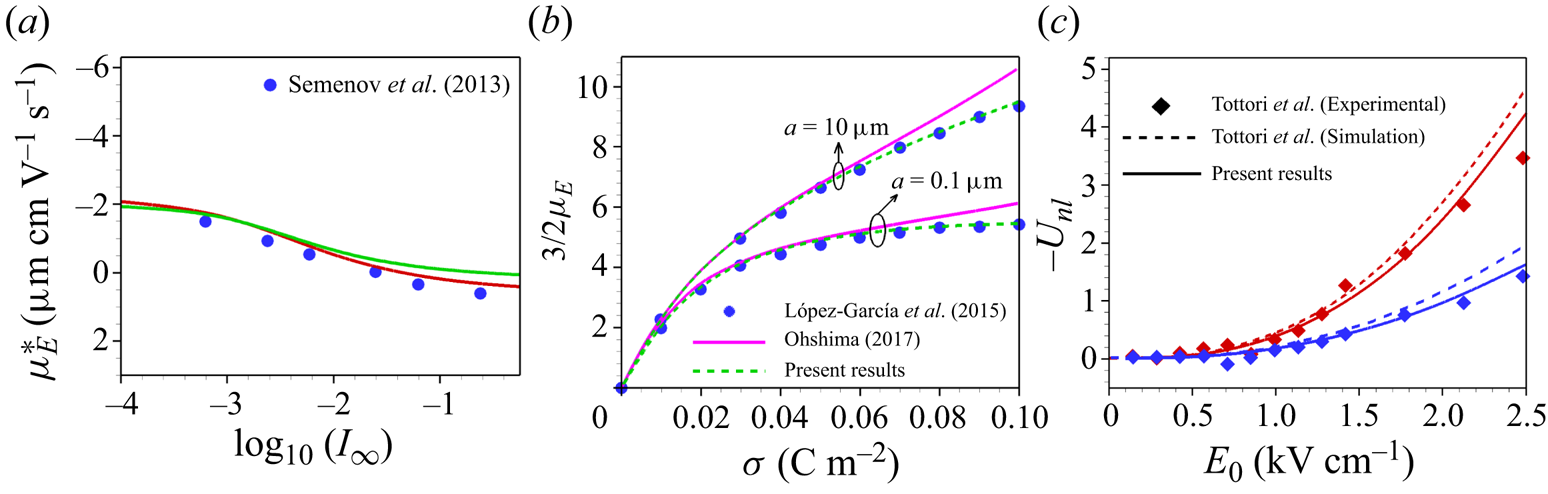
In figure 2(b) we have validated our modified model incorporating the finite-ion-size effect with  $l_c=0$ (in the absence of electrostatic correlations) and constant viscosity (
 $\mu _E=1$) with the theoretical analyses of Ohshima (Reference Ohshima2017) and López-García et al. (Reference López-García, Horno and Grosse2015) and established a close agreement. We have also compared our numerical solutions with the experimental results of Tottori et al. (Reference Tottori, Misiunas, Keyser and Bonthuis2019) for electrophoresis of polystyrene and poly(methyl methacrylate) particles suspended in a KCl electrolyte (figure 2c). Comparison of the nonlinear part of the electrophoretic velocity as a function of the applied electric field is made. The nonlinear part is determined by subtracting the linear electrophoretic velocity, which is determined based on the mobility at a low electric field, from the electrophoretic velocity
 $U_E$. We have also indicated the results based on the numerical simulation of Tottori et al. (Reference Tottori, Misiunas, Keyser and Bonthuis2019) in figure 2(c). A close agreement of our present model with these existing experimental results for a range of
 $E_0$ is encouraging.
We first consider the case of low Péclet number by considering small ions, i.e. ions with larger ion diffusivity, for a moderate range of applied electric field. Based on the thin-layer analysis under a low surface conduction, i.e.  $O(Du)$, Schnitzer & Yariv (Reference Schnitzer and Yariv2014) provided an expression for the mobility of a rigid particle suspended in an electrolyte of small ions as
 \begin{equation} \mu_E=\zeta_0+\overline{Du}\left[{-}4\ln\left(\cosh\frac{\zeta_0}{4}\right)-\zeta_0+\frac{2}{21}\varLambda^{2}\right]. \end{equation}
Here,  $\zeta _0$ is the equilibrium surface potential of the particle surface and it is related to the surface charge density through the relation
 $\zeta _0=2\sinh ^{-1}(\sigma /(2\kappa a))$ and the Dukhin number, as defined by Schnitzer & Yariv (Reference Schnitzer and Yariv2014), is
 $\overline {Du}=(1+2Pe_{i})\sigma /(\kappa a)^{2}$, where
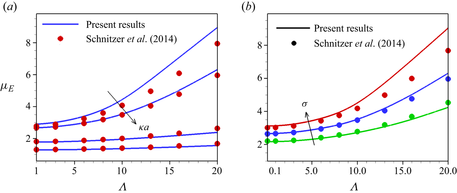
 $Pe_{i}$ is the Péclet number of the counterion. In figure 3 we have compared our numerically determined mobility
 $\mu _E$ based on the PNP model for a small counterion, i.e.
 $Pe_{i}=0.01$, with the expression (5.1) for larger values of
 $\kappa a$ at a fixed
 $\sigma$ (figure 3a) and different
 $\sigma$ at a fixed
 $\kappa a$ (figure 3b). In both cases, we varied the imposed electric field from low to moderate range. We find a good agreement between our computed solutions and the thin-layer analysis at a higher
 $\kappa a$ (thinner EDL) and a deviation from the asymptotic solution for a moderate
 $\kappa a$. A deviation from (5.1) is found at a higher
 $\sigma$ even for a smaller Debye length. In this case the surface conduction becomes stronger. Surface conduction is also stronger at a larger
 $\varLambda$ for a moderate
 $\kappa a$ (
 $=50$), leading to a deviation from the asymptotic solution (5.1).
Comparison of  $\mu _{E}$ based on the present PNP model with the small-ion asymptotic expression (5.1) of Schnitzer & Yariv (Reference Schnitzer and Yariv2014) as a function of the scaled electric field
 $\varLambda$ (a) for different
 $\kappa a\ (=40,50,150,200)$ when
 $\sigma =213$ and (b) for different
 $\sigma \ (=150,213,300)$ and
 $\kappa a=50$. Solid lines, present results; symbols, Schnitzer & Yariv (Reference Schnitzer and Yariv2014).
In order to check the electric field dependence of mobility for a finite Péclet number, we consider the variation of  $\mu _E$ with the imposed electric field for NaCl, KCl and HCl electrolytes in figure 4(a,b), in which the Péclet number
 $Pe_{U_{E}}$ based on the electrophoretic velocity at the highest applied field
 $\varLambda =20$ becomes 20.5, 17.7 and 13.3, respectively. We find that the variation of
 $\mu _{E}$ with
 $\varLambda$ does not follow the pattern given by (5.1) derived for
 $Pe_{U_{E}} \ll 1$. At a higher electric field,
 $\mu _E$ has a strong dependency on the diffusivity of ions. Interestingly, we find that the discrepancy in
 $\mu _E$ due to variation of co-ion diffusivity is stronger than the variation due to the counterion diffusivity. Cobos & Khair (Reference Cobos and Khair2023) have shown by considering the same diffusivity of co-ions and counterions that the ion diffusivity has a negligible impact on the mobility at a lower range of electric field. This impact becomes significant at a higher applied electric field as the number density of ions in the EDL is enhanced. The EDL attracts counterions and creates a repulsion to the co-ions. At a higher
 $\varLambda$ (
 $>1$), for which surface conduction becomes stronger, an asymmetric distribution of ions develops near the outer boundary of the EDL, which creates an induced electric field due to the diffusivity difference of co-ions and counterions. For HCl this diffusivity difference creates a diffusion field aligned with the applied field along
 $z<0$, whereas NaCl creates a diffusion field opposite to the direction of the applied field. For KCl the diffusion field is zero as the diffusivity difference between the ions is almost negligible. This explains the increasing order in
 $\mu _E$ for HCl, KCl and NaCl for the positively charged particle. At a fixed electric field the increment in the nonlinear part of electrophoretic velocity with an increase of diffusivity is in agreement with Schnitzer & Yariv (Reference Schnitzer and Yariv2014). The difference in diffusivity of counterions and co-ions has relatively less impact on the mobility. As the ratio of counterion to co-ion diffusivity decreases, the conductivity of the EDL attenuates, creating an enhancement in
 $\mu _E$, which compensates the loss due to the development of the diffusion field. This leads to less impact on the mobility due to the variation of counterion diffusivity. We find that the MNPC model predicts a higher
 $|\mu _E|$ compared with the PNP model as the hydrodynamic steric interactions in the MNPC model cause a lower accumulation of counterions near the charged surface (figure 4c), which leads to a reduction in screening of the surface charge compared with the PNP model.
Variation of mobility obtained by MNPC and PNP models for NaCl, KCl and HCl with  $\varLambda$ when (a)
 $\sigma =250$ and (b)
 $\sigma =-250$ at
 $\kappa a=50$. Blue lines, NaCl; green lines, KCl; red lines, HCl. Solid lines, PNP; dashed lines with square symbols, MNPC. (c) Variation of counterion concentration with radial distance at
 $\theta ={\rm \pi} /2$ for NaCl electrolyte at
 $\sigma =250$ and
 $\kappa a=50$ when
 $\varLambda =10$.
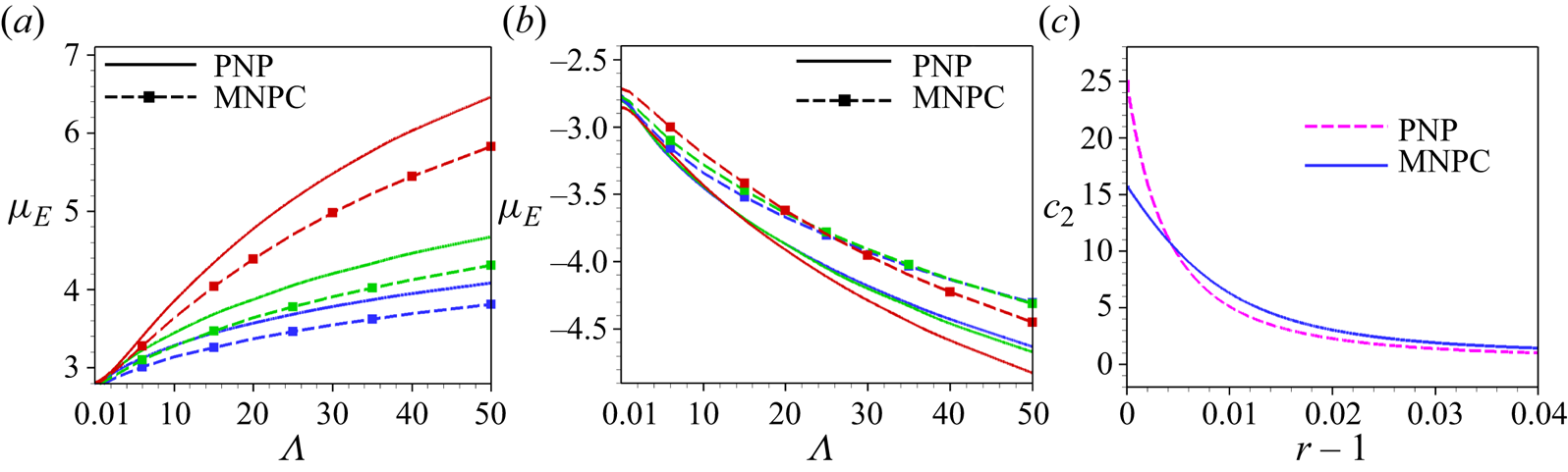
Figure 5(a,b) shows the mobility dependence on the applied field for a thicker ( $\kappa a=10$) and thinner (
 $\kappa a=100$) EDL in monovalent NaCl electrolyte. We present results based on the PNP model as well as the modified MNPC model, which incorporates the finite-ion-size effects and ion correlations. It is evident that the dependence of
 $\mu _E$ on
 $\varLambda$ varies with
 $\kappa a$. We find that the mobility for
 $\kappa a=10$ is independent of
 $\varLambda$ for the lower range of the applied field and then it increases with
 $\varLambda$. This increase in the mobility attenuates at a higher range of
 $\varLambda$. However, the variation of
 $\mu _E$ with
 $\varLambda$ is almost constant for a thinner EDL (figure 5b). The asymptotic analysis of Schnitzer & Yariv (Reference Schnitzer and Yariv2012b) demonstrates a linear dependence of velocity with
 $\varLambda$ up to
 $\varLambda \sim O(\kappa a)$ for a thinner EDL, i.e.
 $\kappa a \gg$1. The experimental study by Lomeli-Martin et al. (Reference Lomeli-Martin, Ernst, Cardenas-Benitez, Cobos, Khair and Lapizco-Encinas2023) also demonstrates a linear dependence of electrophoretic velocity with applied field strength for a higher value of the bulk ionic concentration (i.e.
 $\kappa a \gg 1$). For a moderate range of
 $\kappa a$, i.e.
 $\kappa a\sim O(1)$, an increased electric field creates the driving force exerted on the counterion Na
 $^+$ strong enough to overcome the Coulombic attraction created by the surface charge so that fewer Na
 $^+$ ions screen the surface charge. It also leads to an enhancement of the surface conduction. As the electric field becomes stronger, the number density of co-ions in the diffuse layer increases. This generates a stronger supportive electro-osmotic flow. Combined effects of stronger electric force on the particle and the supportive electro-osmotic flow create a very large increase in mobility. However, the rate of increase in
 $\mu _E$ with
 $\varLambda$ attenuates at a higher range of
 $\varLambda$ and approaches a saturation. This is caused by surface conduction of the particle, which magnifies at a higher
 $\varLambda$. In figure 5(b) we have indicated the analytical solution for
 $\mu _{{HS}}$ governed by (4.26) obtained under a weak applied field and low surface charge density consideration and established a close agreement with the exact numerical solution for a lower range of
 $\sigma ^*$ and
 $\varLambda$ when
 $\kappa a=100$.
Variation of  $\mu _E$ based on the MNPC model as a function of
 $\varLambda$ for (a)
 $\kappa a=10$ and (b)
 $\kappa a=100$ for different
 $\sigma ^*\ (-0.05,-0.1,-0.2\,{\rm C}\,{\rm m}^{-2})$. Black dashed lines,
 $\mu _{{HS}}$ (obtained by (4.26)). (c) Distribution of induced
 $\zeta$ potential at different
 $\varLambda$ (1, 10, 20) when
 $\kappa a=100$ at
 $\sigma ^*=-0.1\,{\rm C}\,{\rm m}^{-2}$ for NaCl electrolyte. (d) Variation of
 $Du$ as a function of
 $\varLambda$ at
 $\kappa a=100$ for different
 $\sigma ^*\ (-0.05, -0.1, -0.2\,{\rm C}\ {\rm m}^{-2}$) for NaCl electrolyte. Solid blue lines, MNPC; dashed red lines, PNP.

The increment in  $\mu _E$ with an increase of
 $\sigma ^*$ may not show a monotonic pattern due to the occurrence of a stronger retarding surface conduction created by the EDL polarization. The results of O'Brien & White (Reference O'Brien and White1978) also show that the mobility enhances with the enhancement of
 $\zeta$ potential until a critical
 $\zeta$ is reached. We find that both the PNP and MNPC models yield the same value of
 $\mu _E$ for a lower range of
 $\kappa a$ and the models differ at a larger
 $\kappa a$. In the MNPC model, the counterion saturation due to steric interactions may attenuate the shielding effect; however, the correlations of ions draw more counterions in the vicinity of the charged surface, amplifying the shielding effect. In addition, the viscosity of the electrolyte near the particle becomes higher in the modified model, creating a higher viscous friction force. These in combination reduce
 $\mu _E$ in the MNPC model as compared with the PNP model. However, at a larger
 $\sigma ^*$ the electric force on the particle becomes high enough to compensate the ion correlative force as well as the excess hydrodynamic friction.
We now illustrate in figure 5(c,d) the influence of the imposed electric field on the  $\zeta$ potential and surface conduction at a smaller Debye length. The induced
 $\zeta$ potential for a small Debye length can be obtained by the difference of electric potential at the surface from the bulk, i.e.
 \begin{equation} \zeta=\phi_s+\frac{3}{2}\varLambda\cos\theta, \end{equation}
where  $\phi _s$ is the computed surface potential. The distribution of
 $\zeta$ potential as depicted in figure 5(c) for a small Debye length
 $\kappa a=100$ shows that it increases as the imposed field is increased. An asymmetric distribution of
 $\zeta$ at a higher
 $\varLambda$ is evident. The electric field lines draw negative ions towards the side facing the electric field (i.e. where field lines terminate) and positive charge on the opposite side from where it originates.
Surface conduction develops due to the transverse flux of ions, which creates a difference in current density in the EDL as compared with the bulk value. The larger applied field attracts an excess amount of ions in the EDL. This excess ionic flux can be measured through the Dukhin number  $Du$ (
 $=(I-I_{\infty })/I_{\infty }$), which can be expressed as
 \begin{align} Du &={-}\frac{1}{\varLambda} \int_0^{\rm \pi} \int_1^{\infty}\left[\sum_{i=1}^2 \frac{z_i D_i}{\sum_{j=1}^2 z_j^2 D_j n_j(\infty)} n_i u -\sum_{i=1}^2 \frac{z_i D_i}{\sum_{j=1}^2 z_j^2 D_j n_j(\infty)} \frac{1}{r} \frac{\partial n_i}{\partial \theta}\right.\nonumber\\ &\quad -\frac{1}{r} \frac{\partial \phi}{\partial \theta} \sum_{i=1}^2 \frac{z_i^{2} D_i}{\sum_{j=1}^2 z_j^2 D_j n_j(\infty)}\left(n_i-n_i(\infty)\right)\nonumber\\ &\left.\quad -\sum_{i=1}^2 \frac{z_i D_i}{\sum_{j=1}^2 z_j^2 D_j n_j(\infty)} \frac{1}{r} \frac{\partial \mu_i^{ex}}{\partial \theta} \right] r^2 \sin \theta \,{\rm d}r\,{\rm d}\theta. \end{align}
We find from figure 5(d) that  $Du$ is negative for a lower range of
 $\varLambda$, i.e.
 $\varLambda <$ 1; then it becomes positive as
 $\varLambda$ becomes larger. Although the counterion concentration near the surface is higher in the PNP model, the EDL in the MNPC model expands. Thus, the region in which the term
 $\sum _{i=1}^{2}z_{i}D_{i}n_{i}$ is non-zero is larger in the MNPC model than in the PNP model. As a result, the contribution of the convective term in
 $Du$ is higher in the MNPC model. Figure 5(d) shows that the surface conduction becomes higher for the MNPC model compared with the PNP model and the difference augments as the surface charge is increased. An enhanced electric field also increases
 $Du$ based on the MNPC model compared with the PNP model. This significant increment in
 $Du$ for the MNPC model creates a reduction in
 $\mu _E$.
The difference in mobility  $\mu _E$ from the mobility
 $\mu _l$ corresponding to a weak applied field (
 $\varLambda =0.1$) measures the nonlinear part of the electrophoretic mobility of the particle, i.e.
 $\mu _{nl}=\mu _E-\mu _l$. Since
 $\mu _{nl}<0$ for the entire range of
 $\varLambda$, this implies that
 $|\mu _E|> |\mu _l|$ for both thinner and thicker Debye length. We find that the variation of
 $\mu _{nl}$ with
 $\varLambda$ depends on the bulk ionic concentration. At a thicker Debye length
 $\mu _{nl}$ increases rapidly with
 $\varLambda$ then it attenuates. For a thinner Debye length this deviation
 $\mu _{nl}$ shows relatively less variation with
 $\varLambda$. At a thicker Debye length an interplay between the surface conduction and shielding of the surface charge leads to a nonlinear variation of
 $\mu _E$ with
 $\varLambda$, which approaches a saturation at a higher
 $\varLambda$. The theoretical study by Rouhi Youssefi & Diez (Reference Rouhi Youssefi and Diez2016) under a low-surface-conduction assumption shows that for
 $Pe \gg 1$ the nonlinear part of the electrophoretic velocity varies as
 $\varLambda ^{3/2}$. However, as mentioned before, the experimental results of Lomeli-Martin et al. (Reference Lomeli-Martin, Ernst, Cardenas-Benitez, Cobos, Khair and Lapizco-Encinas2023) show an almost linear dependence of the electrophoretic velocity with the electric field. At a higher range of
 $\varLambda$ the surface conduction intensifies, which attenuates the rate of increase of
 $\mu _E$ with
 $\varLambda$. We find that
 $\mu _{nl}$ for the MNPC model at a higher range of the bulk ionic concentration becomes negligible. For
 $\kappa a=100$ at
 $\varLambda =20$ the difference
 $\mu _{nl}$ for
 $\sigma ^*=-0.05\,{\rm C}\,{\rm m}^{-2}$ is
 $-$0.165, for
 $\sigma ^*=-0.1\,{\rm C}\,{\rm m}^{-2}$ is
 $-$0.255 and for
 $\sigma ^*=-0.2\,{\rm C}\,{\rm m}^{-2}$ is
 $-$0.79. This implies that the electrophoretic velocity in the MNPC model at a thinner EDL varies linearly with
 $\varLambda$.
We now consider the deviation of  $\mu _E$ for a thinner Debye length from the Smoluchowski mobility
 $\mu _{{HS}}$, i.e.
 $\mu _{sd}=\mu _{{HS}}-\mu _E$. As adopted by Raafatnia et al. (Reference Raafatnia, Hickey, Sega and Holm2014), the
 $\zeta$ potential calculated from the ion distribution in equilibrium can be assumed to be equivalent to that of a system subjected to a weak applied field. Based on the equilibrium
 $\zeta$ potential we obtain the corresponding electrophoretic mobility
 $\mu _{{HS}}$ by (4.19). It may be noted that the Smoluchowski mobility is determined under the condition of no double-layer polarization and relaxation effect. Figure 6(b,c) shows that
 $\mu _{sd}$ for both PNP and MNPC models is close to zero for a lower range of
 $\sigma ^*$. This implies an excellent agreement of
 $\mu _E$ with
 $\mu _{{HS}}$ obtained by (4.19) occurs for smaller range of
 $\sigma ^*$. We find in the PNP model for a higher range of
 $\sigma ^*$ that a large deviation of
 $\mu _E$ from
 $\mu _{{HS}}$ occurs at a smaller value of
 $\varLambda$. This discrepancy reduces as
 $\varLambda$ is increased. This implies that the retardation created by the EDL polarization and relaxation diminishes as the electric field is enhanced. For a monovalent electrolyte,
 $\mu _{sd}<0$ implies
 $|\mu _{{HS}}|>|\mu _{E}|$ as both
 $\mu _E, \mu _{{HS}}<0$. Surprisingly, we find that for a larger electric field
 $\varLambda \ge 10$,
 $|\mu _E|>|\mu _{{HS}}|$ as
 $\mu _{sd}>0$. The situation in which mobility exceeds the value predicted by the Smoluchowski theory is termed superfast electrophoresis (Barany, Mishchuk & Prieve Reference Barany, Mishchuk and Prieve1998). This arises due to the formation of the secondary diffuse charge cloud of counterions drawn by the strong electric fields at the outer surface of the primary EDL induced by the surface conduction. The diffuse layer of counterions produces a slip velocity by the tangential electric field. The occurrence of such slip velocity in the diffuse layer is termed electro-osmosis of second kind (Dukhin Reference Dukhin1991). On the curved surface, the diffuse layer of counterions creates a stronger electric field normal to the surface. The imbalance between the tangential slip velocity and the normal component of velocity may create vortices at the right-hand side of the particle (Demekhin, Shelistov & Polyanskikh Reference Demekhin, Shelistov and Polyanskikh2011; Chang, Yossifon & Demekhin Reference Chang, Yossifon and Demekhin2012; Ganchenko et al. Reference Ganchenko, Frants, Shelistov, Nikitin, Amiroudine and Demekhin2019). At a high enough electric field microvortices may lead to an instability (Chang et al. Reference Chang, Yossifon and Demekhin2012). Our results based on the PNP model do not show any microvortices for the range of parameter values considered in the present study.
(a) Variation of nonlinear component of mobility with  $\varLambda$ for
 $\kappa a=10$ and
 $\kappa a=100$ for different
 $\sigma ^*$ (
 $-0.05, -0.1, -0.2\,{\rm C}\,{\rm m}^{-2}$). Green solid lines,
 $\kappa a =10$ (PNP); black dashed lines,
 $\kappa a =10$ (MNPC); blue solid lines,
 $\kappa a=100$ (PNP); red dashed lines,
 $\kappa a=100$ (MNPC). Variation of mobility deviation (
 $\mu _{sd}$) from Smoluchowski formula obtained by (4.19) as a function of
 $\varLambda$ for (b) PNP model and (c) MNPC model at
 $\kappa a=100$ for different
 $\sigma ^*\ (-0.01,-0.05, -0.1, -0.2\,{\rm C}\ {\rm m}^{-2}$) for NaCl electrolyte. Pink lines,
 $\sigma ^*=-0.01\,{\rm C}\,{\rm m}^{-2}$; red lines,
 $\sigma ^*=-0.05\,{\rm C}\,{\rm m}^{-2}$; green lines,
 $\sigma ^*=-0.1\,{\rm C}\,{\rm m}^{-2}$; blue lines,
 $\sigma ^*=-0.2\,{\rm C}\,{\rm m}^{-2}$.
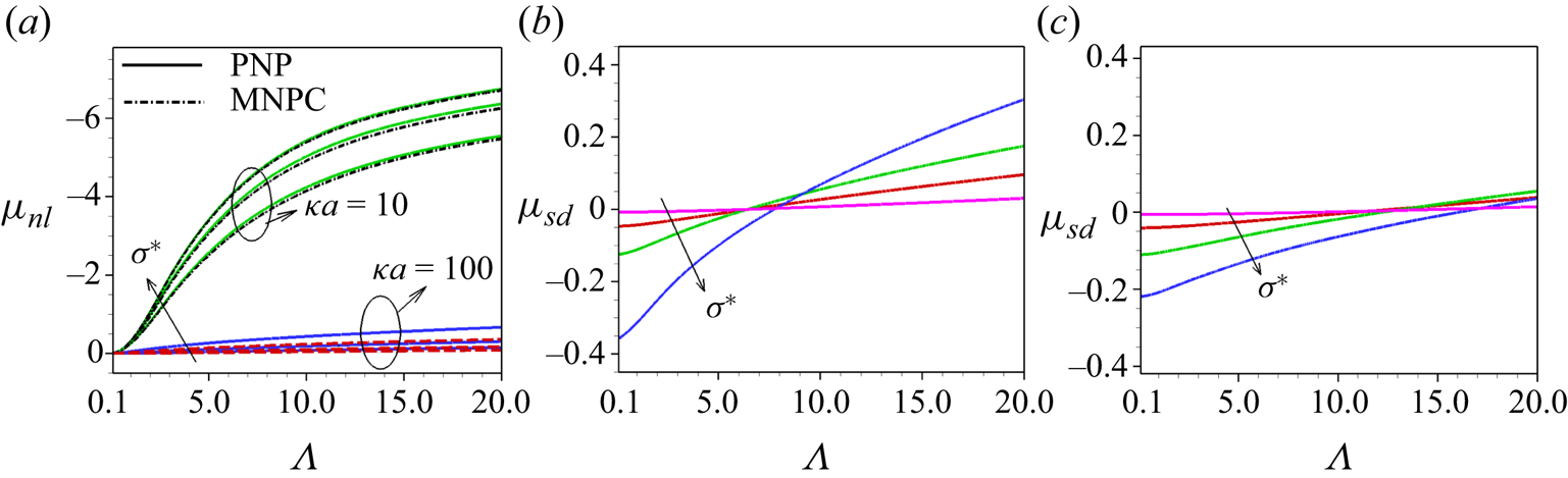
Figure 6(c) depicts the difference in mobility based on the MNPC model from the corresponding Smoluchowski limit  $\mu _{{HS}}$ obtained by (4.19) at different
 $\sigma ^*$ when
 $\varLambda$ is varied. We find that the mobility based on the MNPC model does not exceed that of the corresponding
 $\mu _{{HS}}$ up to a certain range of
 $\varLambda$. The electrostatic correlations and the ion steric interaction create an effective EDL thickness in the MNPC model greater than that in the PNP model. This leads to the impact of Debye layer polarization being stronger in the MNPC model. For this, the deviation from the corresponding Smoluchowski mobility becomes higher. The difference amplifies at a higher
 $\sigma ^*$ as the polarization effect becomes stronger. Unlike the PNP model,
 $\mu _{sd}$ remains relatively invariant due to the variation of
 $\varLambda$. We may remark by comparing figures 6(b) and 6(c) that the electro-osmotic flow of the second kind is suppressed in the MNPC model.
The counterion distribution ( $n_1$), space charge density (
 $\sum _{i}{z_in_i}$) and ionic strength (
 $\tfrac {1}{2}\sum _{i}{z_i^2n_i}$) around a highly charged particle in a monovalent electrolyte at a different applied field are shown in figure 7. An asymmetry in the counterion distribution is evident from the results (figure 7a–c). As
 $\varLambda$ is increased, the counterion-dominated region extends many times beyond the Debye length towards the downstream side of the particle. For the case of larger
 $\varLambda$ the counterion distribution resembles the thermal plume that develops at the downstream of a heated particle in free convection. The strong applied field drags the counterions (positive ions) along the direction of the electric field generating a momentum to the electrolyte medium. The MNPC model shows the development of a counterion condensed layer around the particle. Larger co-ion accumulation at the left-hand side (upstream) of the particle creates a low space charge density. Co-ions accumulate in the EDL creating a lower space charge density compared with the counterion density. The space charge density distribution (figure 7d–f) around the particle shows a spherical symmetry at a lower range of the applied electric field (
 $\varLambda =1$). At a higher range of
 $\varLambda$ a distortion in the charge density around the particle is evident. This implies an occurrence of a significant Debye layer relaxation at a stronger imposed electric field. We find that the charge density intensifies as the electric field is increased, which leads to a higher electric force and, hence, higher velocity at a higher
 $\varLambda$. The ionic strength (figure 7g–i) shows the presence of co-ions at the left-hand side (upstream) of the particle in which the counterion density is low and the space charge density is small. Comparing with figure 7(a–c) for the counterion distribution, we find an accumulation of co-ions adjacent to the counterion plume in the downstream. This reduces the space charge density.
Distributions of counterion (a–c), space charge density (d–f) and ionic strength (g–i) around the particle at  $\varLambda =1$ (a,d,g),
 $\varLambda =10$ (b,e,h) and
 $\varLambda =20$ (c,f,i) when
 $\kappa a=10$ and
 $\sigma ^*=-0.1\,{\rm C}\,{\rm m}^{-2}$ for NaCl electrolyte in the MNPC model.

5.2. Mobility reversal in multivalent electrolyte
The electrostatic correlations become particularly pronounced in the case of trivalent counterions, which overcompensates the surface charge of the particle by excessive adsorption of counterions at the Stern layer. This condensed layer of counterions may overscreen the surface charge, which in turn draws a large number of co-ions in the EDL to make a charge neutrality. The density of co-ions may overwhelm the counterion density in the EDL, leading to a change in the polarity of the EDL. This results in a reversal in mobility of the particle and charge density oscillation. Crowding refers to more than one layer of counterions shielding the surface, which dominates overscreening and results in co-ion excess outside these layers.
The radial profile for the space charge density at the equilibrium situation based on the MNPC model as depicted in figure 8(a) shows a saturation near the particle surface. The space charge density is higher for higher valence of the counterions. For a multivalent electrolyte, the formation of a compact layer of counterions near the particle surface is evident. The charge density sharply declines at the outer side of this compact layer. This compact layer (termed the condensed layer) is induced by the ion–ion correlations formed at the outer surface of the particle and attracts co-ions in the EDL leading to a charge density oscillation. This creates a reversal in the induced electric potential within the EDL at equilibrium (figure 8b,c). We find that the reversal in  $\phi$ becomes prominent for a higher surface charge density. The EDL potential at equilibrium is also affected by the counterion size of the trivalent electrolyte (figure 8c). The surface potential is higher for a larger size of the counterion as the screening effect attenuates due to the stronger ion steric interactions. However, the electrostatic correlation augments for the smaller-sized counterion due to a larger accumulation of counterions in the EDL.
At equilibrium ( $\varLambda =0$) for
 $\kappa a=10$ the radial profile of (a)
 $\rho _e$ for NaCl, BaCl
 $_2$ and LaCl
 $_3$ electrolytes at
 $\sigma ^*=-0.5\,{\rm C}\,{\rm m}^{-2}$. Dashed lines, PNP; solid lines, MNPC. Green lines, NaCl; red lines, BaCl
 $_2$; blue lines, LaCl
 $_3$. Plots of (b)
 $\phi$ at different
 $\sigma ^*\ (-0.01,-0.1,-0.2,-0.5\,{\rm C}\,{\rm m}^{-2})$ for LaCl
 $_3$ electrolyte and (c)
 $\phi$ for different trivalent electrolytes AlCl
 $_3$, LaCl
 $_3$ and Co(NH
 $_3$)
 $_6$Cl
 $_3$ at
 $\sigma ^*=-0.3\,{\rm C}\,{\rm m}^{-2}$.

The variation of mobility with  $\sigma ^*$ for electrolyte LaCl
 $_3$ with trivalent counterion (figure 9a) shows that the magnitude of mobility of the negatively charged colloid reduces and becomes positive as
 $\sigma ^*$ is increased. The electrostatic coupling factor provides a measure of the counterion–counterion interaction with respect to the thermal energy, estimated by the ratio between the Bjerrum length and the Gouy–Chapman length. This coupling constant increases as the surface charge density is enhanced, creating non-negligible correlations between ions. This leads to a formation of a condensed layer of counterions adjacent to the particle surface, which attracts more co-ions in the EDL and an oscillation in the space charge density distribution is found. The stronger condensed layer of counterions screens the surface charge, leading to a reduction in the electric force on the particle. In addition, the accumulation of co-ions in the EDL leads to a reduction in
 $-\mu _E$ and eventually a change of sign in
 $\mu _E$ from negative to positive mobility. Due to the sign inversion in the EDL, co-ions induce liquid flow in an opposite direction to that obtained in classical continuum theory. As pointed out by Stout & Khair (Reference Stout and Khair2014), a zero mobility does not imply a zero effective charge of the particle. It occurs due to the balance of two oppositely attracting electric forces. As described in § 1, the mobility reversal in electrophoresis in a multivalent electrolyte is found experimentally as well as in molecular dynamic simulations and Monte Carlo simulations by several authors (Diehl & Levin Reference Diehl and Levin2006; Kubíčková et al. Reference Kubíčková, Křížek, Coufal, Vazdar, Wernersson, Heyda and Jungwirth2012; Storey & Bazant Reference Storey and Bazant2012; Semenov et al. Reference Semenov, Raafatnia, Sega, Lobaskin, Holm and Kremer2013; Raafatnia et al. Reference Raafatnia, Hickey, Sega and Holm2014; Stout & Khair Reference Stout and Khair2014; Celebi et al. Reference Celebi, Cetin and Beskok2019; Tottori et al. Reference Tottori, Misiunas, Keyser and Bonthuis2019; de Souza et al. Reference de Souza, Goodwin, McEldrew, Kornyshev and Bazant2020; Lomeli-Martin et al. Reference Lomeli-Martin, Ernst, Cardenas-Benitez, Cobos, Khair and Lapizco-Encinas2023). Mobility reversal based on the modified continuum model is also demonstrated by Stout & Khair (Reference Stout and Khair2014) under a first-order approximation, which neglects the polarization of the Debye layer. We find that the mobility approaches a constant at a larger
 $\kappa a$ as the counterions in the EDL attain saturation. In figure 9(b) we provide a comparison of the mobility obtained under the Smoluchowski limit as provided in (4.19) with the computed
 $\mu _E$ at
 $\kappa a=150$ for a wider range of
 $\sigma ^*$. Mobility expression (4.19) for
 $\mu _{{HS}}$ shows a mobility reversal for the lower range of
 $\sigma ^*$, which agrees with the exact numerical results at
 $\kappa a=150$. A larger
 $\sigma ^*$, for which the electric force on the particle becomes strong enough to compensate the retardation created by the co-ion layer in the EDL, creates a negative mobility for the negatively charged particle. We find a close agreement of our exact numerical model with
 $\mu _{{HS}}$ obtained by (4.19) with a deviation by a small margin at a lower range of
 $\sigma ^*$. This implies that the thin-layer analysis cannot capture the counterion condensed layer correctly so that the positive
 $\mu _E$ deviates from the exact numerical solution.
Variation of  $\mu _E$ based on the MNPC model in LaCl
 $_3$ at
 $\varLambda =0.1$ as a function of
 $\sigma ^*$ (a) for different
 $\kappa a$ (
 $30,50,100$), symbols representing the corresponding results of weak-field (W-F) analysis and (b) for
 $\kappa a =150$: blue solid lines,
 $\mu _E$; red dotted lines with symbols,
 $\mu _{{HS}}$ as computed by (4.19). (c) Radial profile electric potential at
 $\theta ={\rm \pi} /2$ for different
 $\kappa a$ (
 $10,20,50,150$) at
 $\varLambda =0.1$ and
 $\sigma ^*=-0.1\,{\rm C}\,{\rm m}^{-2}$ for LaCl
 $_3$ electrolyte. (d) Variation of
 $\mu _E$ based on the MNPC model as a function of
 $\varLambda$ for different
 $\kappa a$ (
 $15,30,50,120$) at
 ${\sigma ^*=-0.1\,{\rm C}\,{\rm m}^{-2}}$ for LaCl
 $_3$.

Figure 9(c) shows that the electric potential changes sign as we move away from the particle. The region of positive potential is created by the formation of a co-ion layer developed due to surface charge overscreening. The formation of such a layer creates a mobility reversal. Without the correlation effect, the space charge density would decay monotonically from the maximum value to zero far from the wall creating a negative  $\phi$ which gradually diminishes to zero at the bulk region. As
 $\sigma ^*$ increases for a moderate range of
 $\kappa a$ the condensed layer of counterions becomes denser and compressed to the charged surface due to the stronger electrostatic interaction with the surface charge, creating a thicker layer of co-ions. However, at a higher
 $\sigma ^*$ for a thinner Debye length the electric force generated by the surface charge overcompensates the counterion correlative force and the negatively charged particle mobility changes its sign from positive to negative. We find that the results based on the simplified model under the weak-field consideration are in excellent agreement with the exact numerical solution. Bazant et al. (Reference Bazant, Storey and Kornyshev2011) has demonstrated that the crowding effect suppresses the overscreening by extending the condensed layer of counterions with multiple ionic sublayers. The suppression of overscreening leads to the reduction in positive mobility as
 $\varLambda$ is increased. This large voltage typically attracts excess amount of ions, and eventually this generates a concentrated solution in the diffuse layer even if the bulk solution is dilute. Figure 9(d) shows that at a high
 $\varLambda$ (
 $=20$),
 $\mu _E$ remains negative as the electric force on the particle becomes stronger than the correlative force created by the counterions. As
 $\kappa a$ increases, the condensed layer of counterions becomes thinner and denser to create a stronger shielding effect on the surface charge, and reduces the co-ion concentration in the EDL. This leads to an attenuation of positive
 $\mu _E$ and suppression of mobility reversal at a sufficiently large
 $\kappa a$. The variation of
 $\mu _E$ with
 $\varLambda$ amplifies as the Debye length is increased.
The counterion saturation for monovalent and multivalent counterions and the development of a condensed layer for multivalent ions are illustrated in figure 10(a) by presenting the radial profile of the space charge density. We find that the present modified MNPC model demonstrates the counterion saturation near the charged surface. The PNP model shows an unbounded growth in  $\rho _e$ as we approach the surface of the particle. The MNPC model shows the formation of a condensed layer of counterions for the BaCl
 $_2$ and LaCl
 $_3$, whereas, for the monovalent NaCl,
 $\rho _e$ gradually decays to zero as we move away from the particle surface. At the outer side of the condensed layer, a region of
 $\rho _e>0$ develops for the multivalent counterions, arising due to the overscreening of the surface charge. This co-ion-dominated zone is prominent for LaCl
 $_3$ compared with BaCl
 $_2$. The radial distribution of the space charge density for different ion sizes is presented in figure 10(b), which shows that for electrolyte with a higher counterion size the ion steric effect is stronger, leading to a lower
 $\rho _e$ near the charged surface. This stronger crowding effect attenuates the overscreening, creating a smaller zone of positive
 $\rho _e$ as the ion size is increased.
Variation of  $\rho _e$ with the radial distance at
 $\theta ={\rm \pi} /2$ for (a) NaCl, BaCl
 $_2$ and LaCl
 $_3$ electrolytes at
 $\sigma ^*=-0.5\,{\rm C}\,{\rm m}^{-2}$,
 $\kappa a =50$ and
 $\varLambda =0.1$. Green lines, NaCl; red lines, BaCl
 $_2$; blue lines, LaCl
 $_3$. (b) For different trivalent electrolytes AlCl
 $_3$, LaCl
 $_3$ and Co(NH
 $_3$)
 $_6$Cl
 $_3$ when
 $\varLambda =0.1$,
 $\sigma ^*=-0.4\,{\rm C}\,{\rm m}^{-2}$ and
 $\kappa a=100$. (c) For
 $\kappa a =10$ based on different choice of
 $\delta _{c}$ at
 $\sigma ^*=-0.5\,{\rm C}\,{\rm m}^{-2}$ and
 $\varLambda =0.1$. Green lines,
 $\delta _{c}$ by formula (2.9); red lines,
 $\delta _{c}=d_{ion}\kappa$; blue lines,
 $\delta _{c}=2\kappa (1/l_{B}+1/d_{ion})^{-1}$. Dashed lines, PNP model; solid lines, MNPC model.

In figure 10(c) we have tested the effect of different forms of  $l_c$, namely
 $l_c=d_{ion}$, harmonic mean between
 $d_{ion}$ and
 $l_B$ as well as
 $l_c$ obtained by the power-law formula (2.9). We find that the pattern in the radial profile is similar for all cases. However,
 $l_c$ based on the formula (2.9) provides less overscreening compared with the other choices of
 $l_c$. The mobility for different choices of
 $l_c$ is
 $\mu _E= 3.0106$, 3.1221 and 2.9494, respectively. This justifies that
 $l_c$ based on (2.9) is appropriate for analysing the ion–ion correlations for a higher
 $c_0$ in which the ion crowding effect manifests.
We now present the space charge distribution and streamlines based on the two different models. Results based on the PNP model show that the negatively charged particle has negative mobility for all the cases considered. The space charge density is positive near the negatively charged particle and the negative co-ions are repelled by the surface charge. The mobility based on the MNPC model is negative for the negatively charged particle for a lower range of the electric field. The space charge density contours show the formation of a condensed layer of counterions in the vicinity of the surface. This condensed layer draws co-ions in the EDL, which is evident from figure 11(b). The counterion condensed layer becomes more compact and close to the particle due to the stronger electrostatic force by the higher surface charge density of the particle. At a higher electric field the negatively charged particle migrates along the  $z<0$ direction and a counterion plume develops. The condensed layer of counterions and accumulation of co-ions in the EDL are evident from figure 11(c).
Distribution of space charge density ( $\rho _e$) and streamlines around the particle for (a)
 $\varLambda =1$ in PNP model, (b)
 $\varLambda =1$ in MNPC model and (c)
 $\varLambda =20$ in MNPC model when
 $\kappa a=10$ and
 $\sigma ^{*}=-0.1\,{\rm C}\,{\rm m}^{-2}$ for LaCl
 $_3$ electrolyte.

The space charge density  $\rho _e$ (
 $= \sum {z_i n_i}$) distribution on the surface
 $(r=1)$ at different
 $\varLambda$ shows an asymmetric distribution around the surface and this asymmetry amplifies as
 $\varLambda$ is increased. The concentration of the mobile counterions enhances as
 $\varLambda$ is increased, which creates a stronger surface conduction. This asymmetry in
 $\rho _e$ creates EDL polarization. An oscillation in space charge density is evident from figure 12(b). As the bulk ionic concentration is increased, the condensed layer of counterions becomes thinner (figure 12c).
Variation of space charge density  $\rho _e$ in LaCl
 $_3$ electrolyte (a) over the particle surface for
 $\kappa a =10$; and with the radial distance at
 $\theta ={\rm \pi} /2$ for (b)
 $\kappa a =10$ and (c)
 $\kappa a =100$. Here
 $\varLambda =1,10,20$ and
 $\sigma ^*=-0.1\,{\rm C}\,{\rm m}^{-2}$ in the MNPC model.

Mobility variation with  $\varLambda$ at a thicker EDL, i.e.
 $\kappa a=10$ (figure 13a), is different from the corresponding variation at
 $\kappa a=100$ (figure 13b). Mobility based on the MNPC model enhances rapidly with
 $\varLambda$ and then the increase slows down at higher
 $\varLambda$. This attenuation in the increase of
 $\mu _E$ with
 $\varLambda$ occurs at a relatively lower value of
 $\varLambda$ for a smaller surface charge density. This pattern of variation of
 $\mu _E$ with
 $\varLambda$ is similar to that of the corresponding monovalent electrolytes, as described in figure 5(a). At a low surface charge, the counterion concentration is not high enough to make the correlation effects significant so that the mobility remains negative. Mobility shows a reversal, i.e. negative to positive, at a lower range of
 $\varLambda$ for which overscreening due to electrostatic correlations is significant. It is interesting to note that at a higher
 $\sigma ^*$ the positive
 $\mu _E >$ 0 enhances with
 $\varLambda$ for a smaller range of
 $\varLambda$. Further increase in
 $\varLambda$ reduces
 $\mu _E$ and it becomes negative at a higher
 $\varLambda$. Enhancement in
 $\mu _E$ with
 $\varLambda$ occurs due to a larger accumulation of co-ions in the EDL, which creates an alteration of the EDL charge leading to
 $\mu _E>$ 0. Further increase of
 $\varLambda$ creates an electrostatic force strong enough to overcome the space charge density reversal to create
 $\mu _E<$ 0. However, at a thinner EDL (figure 13b) the overscreening diminishes as the electric field
 $\varLambda$ is increased. In this case the accumulation of co-ions outside the condensed layer in the EDL is insignificant so that no mobility reversal occurs. We find that the rate of enhancement in
 $\mu _E$ with
 $\sigma ^*$ at a thinner Debye length attenuates as
 $\varLambda$ is increased. This could be due to the interplay between the increasing correlation effects and the electrostatic force on the particle at a higher
 $\sigma ^*$ for a larger
 $\varLambda$. We find that the mobility based on (4.19) for the Smoluchowski limit becomes invalid for a higher range of
 $\varLambda$. However, the difference in
 $\mu _E$ from
 $\mu _{{HS}}$ does not show a similar pattern when
 $\sigma ^*$ is varied. This shows that the electrophoresis of a second kind develops at a larger
 $\varLambda$ depending on the surface charge density. In contrast with the monovalent electrolyte, here we find that the deviation of
 $\mu _{{HS}}$ from
 $\mu _E$ magnifies as
 $\varLambda$ increases. This is due to the fact that
 $\mu _{{HS}}$ does not consider the suppression of overscreening by the ion crowding effect arising at a higher range of the electric field. This effect is less pronounced in the monovalent electrolyte.
Variation of  $\mu _E$ with
 $\varLambda$ for (a)
 $\kappa a=10$ and (b)
 $\kappa a=100$ at different
 $\sigma ^{*}\ (-0.01,-0.05,-0.1,-0.2\,{\rm C}\,{\rm m}^{-2})$ for LaCl
 $_3$. Variation of
 $\mu _E$ with
 $\varLambda$ for different trivalent electrolytes AlCl
 $_3$, LaCl
 $_3$ and Co(NH
 $_3$)
 $_6$Cl
 $_3$ when (c)
 $\kappa a=10$ and (d)
 $\kappa a=100$ at
 $\sigma ^*=-0.08\,{\rm C}\,{\rm m}^{-2}$. Dashed lines, Smoluchowski mobility computed by (4.19).

The effect of the counterion size on the particle mobility based on the MNPC model is presented in figure 13(c,d) for a thicker as well as thinner Debye length. We find that the counterion size has a strong effect on the electrostatic correlation. The steric force for a larger-sized counterion is higher leading to less accumulation of counterions near the charged surface. This leads to a reduced surface charge screening and, hence, an increased  $\zeta$ potential for larger ions. We find that the magnitude of the negative mobility is in increasing order of the counterion size, i.e. Co(NH
 $_3)_6^{3+} < \text {La}^{3+} < \text {Al}^{3+}$. However, the electrostatic correlation effect created by the counterions becomes greater when the ionic diffusivity becomes larger for smaller-sized counterions, as the number density of counterions is higher. For this we find that the positive
 $\mu _E$ is higher for a lower-sized counterion. These impacts augment as the bulk ionic concentration is increased. We find that
 $\mu _{{HS}}~ (>0)$ also becomes higher for smaller-sized counterions.
6. Conclusion
We adopted a modified continuum model (MNPC) incorporating finite-ion-size effects and ion correlation contribution to analyse nonlinear electrophoresis for both  $z:z$ and non-
 $z:z$ electrolytes. The hydrodynamic steric interactions of ions are modelled through the BMCSL equation and the medium viscosity is considered to vary with the local ionic volume fraction. The ion correlation contribution is considered by accounting for the non-local part in the electrostatic free energy of ions. This leads to a fourth-order Poisson–Fermi equation for the electric potential, which involves a parameter, the correlation length (
 $l_c$). The present model is validated by comparing it with existing experimental data for electrophoresis in a LaCl
 $_3$ electrolyte and captured the mobility reversal at a higher ionic concentration. We have established a close agreement with existing experimental results for a monovalent electrolyte in which the imposed electric field is varied up to
 $2.5\times 10^5\,{\rm V}\,{\rm m}^{-1}$. The present modified model (MNPC) reduces to the standard point-charge-based PNP model when the ion size and
 $l_c$ are set to zero. Our PNP model agrees well with the existing theory of electrophoresis at a strong electric field for small ions.
We find that for a monovalent electrolyte, the discrepancy of the present model from the PNP model is insignificant up to a moderate range of EDL thickness, i.e. EDL thickness of the order of the particle size:  $\kappa a \sim O(1)$. For
 $\kappa a \gg 1$ the finite-ion-size effect becomes prominent, creating a higher
 $\zeta$ potential than for the PNP model. However, the mobility can become lower than the corresponding mobility based on the PNP model due to the enhancement of the medium viscosity. The rate of increment in mobility with the applied electric field attenuates in the MNPC model. Overscreening and mobility reversal are found for a trivalent electrolyte, in which the correlation length is larger. At a higher applied electric field, the overscreening of the surface charge is compensated by the enhanced electric force at the particle, which may suppress the mobility reversal. In a multivalent electrolyte, a condensed layer of counterions develops on the particle surface, which attracts co-ions, creating an extension in the EDL. An enhanced electric field draws more ions in the EDL and the condensed layer of counterions expands. This leads to the ion crowding effect and suppression of overscreening. However, the overscreening and mobility reversal may occur in a trivalent electrolyte at a larger electric field in which the surface charge density can create a electrostatic force to the condensed layer strong enough to overcome the force exerted by the applied electric field.
A simplification of the present MNPC model is made under a weak applied electric field consideration. This simplified model involves a set of ordinary differential equations, which can be solved through any easily available software or through a central difference scheme. This simplified model is shown to be identical to the exact numerical model for a lower range of the applied electric field. From this model we have derived the corresponding Smoluchowski limit of the mobility, which shows that a reversal in mobility can occur for a non-zero value of the correlation length. The present weak-field model can provide a benchmark for the measurement of electrophoresis of a highly charged colloid in a charged asymmetric electrolyte.
We find that the present continuum-based MNPC model successfully captures the short-range effects such as ion crowding, overscreening of surface charge, oscillation in EDL charge density and reversal in mobility during electrophoresis. However, this model is sensitive to the correlation length and the additional boundary condition on electric potential at the charged surface. Further study on these aspect is needed to make the model more robust and precise.
Funding
Financial support from the Science and Engineering Research Board, Government India (grant no. CRG/2022/005758) is gratefully acknowledged.
Declaration of interests
The authors report no conflict of interest.
Appendix. Outer boundary size
The dependence of domain size  $R$ on the mobility
 $\mu _E$ for a wide range of the applied electric field
 $\varLambda$ is illustrated in figure 14(a,b) at a thicker (
 $\kappa a=3$) and a thinner (
 $\kappa a=50$) Debye length.
Impact on  $\mu _E$ due to the variation of the outer boundary
 $R$ when
 $\varLambda \leq 50$ at (a)
 $\kappa a=3$ when
 $\sigma ^*=-0.01\,{\rm C}\,{\rm m}^{-2}$ and (b)
 $\kappa a=50$ when
 $\sigma ^*=-0.1\,{\rm C}\,{\rm m}^{-2}$.


 Open access

