NOMENCLATURE
- a 1
constant in Reynolds stress formula
- C f
friction coefficient
- C p
pressure coefficient
- c
aerofoil chord
- D
open jet wind tunnel jet width
- kt
turbulence kinetic energy
- R k, R β, R ω
turbulence model constants
- Re
Reynolds number
- S ij
mean strain tensor
- T i
turbulence intensity
- t
time
- U, V, W
time averaged velocity components in x, y and z directions
- x, y, z
Cartesian coordinates
Subscripts
- c
based on aerofoil chord
- High
high velocity side of a mixing layer
- Inlet
specified at the computational domain’s inlet
- Low
low velocity side of a mixing layer
- ref
reference
- rms
root mean squared
- VO
relating to the free shear layer’s virtual origin
- θ
based on shear layer’s momentum thickness
Superscripts
- +
expressed in viscous units
Greek symbol
 $$\mathop \alpha \nolimits_0 ,\alpha _0^*,\mathop \alpha \nolimits_2 ,\alpha _2^*$$
turbulence model constants
- $$\mathop \alpha \nolimits_1 ,\alpha _1^*,\beta _1^*$$
turbulence model variables
- $$\mathop \beta \nolimits_1 ,\mathop \beta \nolimits_2 ,\beta _2^*$$
turbulence model constants
- Δt
time step
- ε
turbulence dissipation rate
- κ
turbulence model constants
- μ
molecular viscosity
- μ t
turbulent eddy viscosity
- ν
kinematic viscosity
- ν t
turbulent kinematic viscosity
- ν eff
effective kinematic viscosity, ν + ν t
- σ k1, σ k2, σ ω1, σ ω2
turbulence model constants
- τ ij
Reynold stress tensor
- Ω
magnitude of vorticity
- Ω ij
vorticity tensor
- ω
dissipation per unit turbulence kinetic energy, ε/(β*k t)


1.0 INTRODUCTION
Open jet wind tunnels are at the centre of the experimental effort to investigate the physics of aerofoil noise production. The complexity of the open jet flow field often leads to significant interaction between the aerofoil and the open jet, creating some uncertainty with regards to the collected data. There is rising demand for more accurate open jet experiments to meet the increasingly stringent legislation being introduced to govern civil aircraft noise. Hence, the ability to predict facility interaction would be valuable in the design of open jet experiments and would enable improved understanding and analysis of the acquired data.
The simplest possible open jet flow is obtained when the potential core of the jet, the working section, is empty and the flow field becomes essentially that of a planar jet. In the absence of any restriction on the jet’s development, it can be decomposed in accordance with Bradshaw et al. (Reference Bradshaw, Ferriss and Johnson1) designation for a round jet. When an aerofoil is placed in the potential core of the open jet, the breakdown of the flow field is modified to reflect the aerofoil’s interaction with the free shear layers, as shown in Fig. 1. The extent and severity of the interaction in the mixing layer’s approximate self-similarity region depends on the chosen aerofoil profile and its position inside the working section.
Open jet flow field with aerofoil installed, (modified from Fig. 1a in Bradshaw et al.(Reference Bradshaw, Ferriss and Johnson1)).

Building on the findings and observations of Brooks et al. (Reference Brooks, Marcolini and Pope2) and Moreau et al. (Reference Moreau, Henner, Iaccarino, Wang and Roger3), Al-Shabab(Reference Al-Shabab4) used LES to investigate open jet installation effects with a model of the open jet facility included in the LES domain. Different aspects of the aerodynamic interaction were discussed, with emphasis on the impact of the expanding free shear layers on the aerofoil’s near field, mainly blockage effects and the increase in background disturbances inside the working section.
While high-fidelity simulations provide an insight into poorly understood flow physics, it is often not feasible to use them repetitively to compare many different configurations. Thus, from a practical perspective, it would be useful to validate a cheaper strategy that has the capability of assessing the relative installation impact under different open jet configurations.
In spite of recent advances in turbulence modeling, RANS models remain an attractive option in Computational Fluid Dynamics (CFD) studies due to their low computational requirements, their availability in many fluid flow solvers and the accumulated experience in their application. They provide a compromise between cost and information, making them a popular choice in optimisation and parametric studies. Hanjalic(Reference Hanjalic5) noted that the availablitiy of greater computational power tends to reduce the design cycle timescale rather than promote a substantial shift away from RANS towards more computationally demanding methods. Hence, and in contrast with some previous forecasts, Hanjalic(Reference Hanjalic5) concluded that RANS models are likely to remain in widespread use in industry for the foreseeable future.
The present study will focus on Menter’s SST model(Reference Menter6), nevertheless, any aerospace oriented RANS model that has been developed for complex flows involving aerofoils, mixing layers, wakes and jets could have been chosen. Menter’s SST model has a slight advantage in benefiting from the many corrections devised for the k − ω and k − ∊ models.
The main objective of the present work is to evaluate the performance of the chosen RANS model, the Menter SST model, when applied to the open jet aerofoil interaction problem. The underlying incentive is to build upon the available LES data and laboratory measurements to establish confidence in a simple, quick turnaround modeling strategy that could be incorporated into the design of open jet experiments. Given this outlook, the bias here is towards reduced complexity and increased accessibility, where possible.
The presentation of results and discussion will focus in turn on the two main regions of the open jet flow field:
• The aerofoil’s nearfield consisting of the boundary layer developing on the aerofoil’s surface and the near wake region. Obtaining the desired aerofoil loading is essential in the assessment of the impact of the open jet environment and choosing representative flow conditions that allow the study of the phenomena of interest.
• The free shear layers, whose development and possible deflection leads to significant blockage in the working section and contain high-turbulence intensity leading to background disturbances or buffeting affecting the working section incrementally on moving downstream.
2.0 NUMERICAL METHODS
2.1 Flow field solver
The open source solver OpenFOAM was used to conduct the present investigation. OpenFOAM is a collection of C++ libraries that provides a variety of fluid flow simulation tools(Reference Jasak7). Many of the popular RANS turbulence models and the main numerical schemes used to solve fluids problems are available as part of the standard OpenFOAM distribution. The current investigation was conducted using OpenFOAM-2.2.2 as the starting point with some modifications applied to certain turbulence models, as will be discussed later.
OpenFOAM uses a finite volume unstructured framework which simplifies the treatment of complex geometries. The governing equations are solved in their integral form as described by Equations (1) and (2), for the incompressible case. Many options are available for the descretization of temporal and spacial derivatives depending on the simulation type.
 $$\int_V \nabla \cdot \bar udV = 0$$
 $$\matrix{
{\int_t^{t + \Delta t} \left[ {{d \over {dt}}\int_V \bar udV + \int_V \nabla \cdot \left( {\bar u\bar u} \right)dV - \int_V \nabla \cdot {\nu _{eff}}\left( {\nabla \bar u + \nabla {{\bar u}^T}} \right)dV} \right]dt} \cr
{ = - \int_t^{t + \Delta t} \left[ {{1 \over \rho }\int_V \nabla \bar pdV} \right]dt} \cr
} $$
In steady RANS simulations, a second order upwind differencing scheme is used for the non-linear convective term of the transport equations, while the viscous term is discretised using a second order central difference scheme. The simulations were conducted using a SIMPLE algorithm(Reference Patankar and Spalding8) and their convergence was monitored through the decay of residuals and integrated forces on the aerofoil reaching a constant value.
2.2 RANS model modifications and corrections
The Menter SST RANS model(Reference Menter6) is a two-equation model designed to simulate fully turbulent flows. After evaluating the performance of the original model, Wilcox(Reference Wilcox9) low-Re correction was introduced in order to improve the prediction of boundary layer development on the suction surface. In addition, a vorticity based formulation of the production term was used(Reference Menter, Kuntz and Langtry10) and sustaining terms,  $${\beta ^ \star }{\omega _{{\rm{I}}nlet}}{k_{{\rm{I}}nlet}}$$ and
 $$\beta \omega _{{\rm{I}}nlet}^2$$(Reference Spalart and Rumsey11) were added to the k and ω transport equations respectively, for controlled decay of turbulence transport variables.
2.2.1 Low Reynolds number modification
The key feature of interest here is the critical Reynolds number at which the production of turbulence exceeds dissipation in the transport equations. This, in effect, relates to the k − ω model that is applied near viscous surfaces in the Menter’s SST model formulation. The process is described in detail by Wilcox(Reference Wilcox9), with the important conclusion that the model transitions at a lower critical Reynolds number than is observed physically.
Wilcox (Reference Wilcox9, Reference Menter, Ferreira, Esch and Konno12) proposed a low-Re modification that improves the model’s behaviour in the lower Reynolds number range by increasing its critical Reynolds number to match better the results of a flat plate boundary layer with a zero pressure gradient. This modification was incorporated into the framework of the Menter SST model in the work of Menter et al. (Reference Menter, Ferreira, Esch and Konno12) and Langtry(Reference Langtry13). The improvement is achieved by introducing damping functions for some of the constants in the k − ω model based on the turbulent to molecular viscosity ratio.
 $${R_t} = {{{\nu _t}} \over \nu } = {k \over {\omega \nu }}$$
The eddy viscosity equation becomes
 $${\nu _t} = {\rm{m}}in\left[ {{\alpha ^ \star }{k \over \omega },{{{a_1}k} \over {\Omega {F_2}}}} \right]$$
where the near wall model constants in the new formulation are
 $$\matrix{
{\alpha _1^ \star = {{\alpha _0^ \star + {{{R_T}} \over {{R_k}}}} \over {1 + {{{R_T}} \over {{R_k}}}}},\quad \quad {\alpha _1} = {5 \over 9}{{{\alpha _0} + {{{R_T}} \over {{R_\omega }}}} \over {1 + {{{R_T}} \over {{R_\omega }}}}},\quad \quad \beta _1^ \star = 0.09{{{5 \over {18}} + {{\left( {{{{R_T}} \over {{R_\beta }}}} \right)}^4}} \over {1 + {{\left( {{{{R_T}} \over {{R_\beta }}}} \right)}^4}}}} \cr
{{\sigma _{k1}} = 0.85,\quad {\sigma _{\omega 1}} = 0.5,\quad {\beta _1} = 0.075,\quad \alpha _0^ \star = {{{\beta _1}} \over 3},\quad {\alpha _0} = 0.1,\quad a1 = 0.31} \cr
{{R_k} = 6,\quad {R_\omega } = 2.7,\quad {R_\beta } = 8} \cr
} $$
while the far field model constants in the new formulation are
 $$\matrix{
{{\sigma _{k2}} = 1.0,\quad {\sigma _{\omega 2}} = 0.856,\quad {\beta _2} = 0.0828,\quad \kappa = 0.41} \cr
{\beta _2^ \star = 0.09,\quad \alpha _2^ \star = 1.0,\quad {\alpha _2} = {{{\beta _2}} \over {\beta _2^ \star }} - {\sigma _{\omega 2}}{{{\kappa ^2}} \over {\sqrt {\beta _2^ \star } }}} \cr
} $$
The near wall and outer flow constants are combined using the standard Menter blending function, so that α *, for example, is obtained from the values of  $$\alpha _1^ \star $$ and
 $$\alpha _2^ \star $$
 $$\phi = {F_1}{\phi _1} + (1 - {F_1}){\phi _2}$$
In addition, the switching function between the two models requires modification to ensure that the k − ω model is the one applied in the boundary layer. This is achieved by redefining the blending function using a wall distance based turbulent Reynolds number as in Biswas and Fukuyama(Reference Biswas and Fukuyama14) and Menter et al. (Reference Menter, Ferreira, Esch and Konno12).
 $${R_y} = {{y\sqrt k } \over \nu }$$
with F 1 becoming
 $${F_1} = max\left( {{F_{1orig}},{F_4}} \right),$$
where
 $${F_4} = \exp \left[ { - {{\left( {{{{R_y}} \over {120}}} \right)}^8}} \right]$$
It is worth clarifying at this stage that the concept of boundary layer transition, which is used frequently in the discussion of results, refers to slightly different processes in the framework of RANS and LES, reflecting the differences between the two strategies in modeling boundary layer development. Transition in the context of high-Re RANS models is a pure mathematical modeling phenomenon that in the case of the Menter SST model starts with a sharp rise in the production of turbulence kinetic energy term, continues through the rise in the production of specific dissipation rate term and usually ends when the kinetic energy production and dissipation balance each other. This process is described thoroughly in Wilcox(Reference Wilcox9). Most RANS models are developed for high Reynolds number fully turbulent flows where this mathematical transition process occurs rapidly near the leading edge of the geometry of interest. On the other hand, wall resolving LES attempts to capture the physical mechanisms that lead to boundary layer transition, so that LES transition more directly reflects the flow physics. That being the case, the potential of RANS could be greatly improved if its mathematical transition can be more tightly linked to the relevant flow physics, which is the purpose of the implemented low-Re correction.
3.0 COMPUTATIONAL SETUP
The computational setup is based on the experimental configuration of Winkler et al. (Reference Winkler, Moreau and Carolus15). Moreau et al. (Reference Moreau, Henner, Iaccarino, Wang and Roger3) emphasised the importance of modeling the open jet facility in numerical investigations, hence a model of the open jet wind tunnel is included in present simulations, which is similar to the one used successfully in a previous investigation by the authors(Reference Al-Shabab4), wherein the nozzle contraction is modelled by a constant area duct with inviscid inner walls.
Jet flows entrain mass from their surroundings. This process is often accounted for by introducing a negligible co-flow in jet simulations(16–19). If the surrounding fluid is stagnant in a computational simulation, then the entrainment process depends on the boundary condition implementation. However, introducing a co-flow of approximately 1% of the jet velocity makes the simulations more stable and robust, particularly in time dependent computations. The introduction of a co-flow is especially suitable in cases where interest is restricted to areas within two or three jet widths from the nozzle exit, since the jet core velocity remains much larger than the co-flow in that region.
The general case setup and boundary conditions are illustrated in Fig. 2. The values of the different velocity components, as well as the turbulence model transport variables, are specified at the inlet boundary, while static pressure values are extrapolated from the internal field. On the other hand, the static pressure values are set at the outflow boundary and the values of the other primitive variables are extrapolated from the internal field.
General case layout and boundary conditions.

Three two-dimensional grids, of different resolution, were designed to conduct the open jet simulations and a grid independence study. The size of the three grids is given in Table 1.
The experimental Mach number of 0.062 provides a justification for the use of an incompressible solver. The Reynolds number is set equal to that of the experimental study at 1.9 × 10⁵ with an aerofoil chord, c, of 0.135 m and a jet velocity of 21.2 ms−1. When it is required to trip the aerofoil’s boundary layer, a step trip is used with a square cross section placed at 10% chord on both surfaces, see Fig. 3.
Details of the Grids Used to Test Grid Independence

Boundary layer trip on suction and pressure surfaces.

The boundary conditions at the inflow are set to reflect the low turbulence intensity at the open jet’s nozzle exit, which is typical of most aeroacoustic facilities(Reference Mueller20). This is consistent with the experiment of Winkler et al. (Reference Winkler, Moreau and Carolus15) in which the turbulence intensity measurement at nozzle exit was reported to be Ti < 0.2%. The exact values used in the RANS simulations will be given in the results section.
The simulations were run on a high performance computing cluster utilising Intel Sandy Bridge E5-2670 processors. The CPU hours required to run the RANS simulations on Grids 1, 2 and 3 were approximately 20, 6 and 1 respectively, while the wall resolved LES(Reference Al-Shabab4) used around 65000 CPU hours.
4.0 RESULTS
4.1 Grid independence
While it is desirable to take advantage of the lower spatial discretization requirements of RANS, it is necessary to ensure that the solution remains grid independent. Therefore, the three grids described in Table 1 above were tested with Menter’s SST turbulence model, which will be the starting point of the current investigation, to obtain the distribution of aerodynamic ntities over the aerofoil and the turbulence kinetic energy profile in the free shear layer above the aerofoil’s leading edge for each of the three grids.
The results are presented in Fig. 4 for the pressure distribution, skin friction and turbulence kinetic energy profile. Comparing the results confirms that the grid does not have any significant effect on the solution. Therefore, it is possible to proceed with the RANS study using Grid 3 in Table 1.
Grid sensitivity study.

An interesting feature of the aerofoil profile used in this investigation (NACA 6512-63) is that, when placed at zero incidence in the open jet wind tunnel, it produces a suction peak with a steep adverse pressure gradient near the leading edge of the pressure surface, resulting in a flip of relative pressure values between the two surfaces further downstream along the chord. The pressure surface values are marked in Fig. 4a with sres over the lines to help distinguish them from the suction surface. Subsequent pressure distribution figures will not have separate markings for the two surfaces, but should be easy to follow henceforth.
4.2 Aerofoil’s nearfield development
Initially, the standard Menter SST RANS model is applied to the open jet configuration. It should be noted that the chord based Re in this case (Rec = 1.9 × 10⁵) is somewhat intermediate between the high Re regime 𝒪(106), which most standard aerospace-oriented RANS models have been designed for, and the low Re regime 𝒪(104), in which standard models have been shown to encounter difficulties(Reference Rumsey and Spalart21,Reference Catalano and Tognaccini22). Furthermore, the boundary layer trip that was placed at 10% chord in the experiment might not be necessary in RANS simulations. Therefore, it is prudent to test the Menter SST model’s behaviour over a wide range of inlet boundary conditions in the presence and absence of a trip, in order to establish a better understanding of its behaviour under various conditions. The inflow RANS boundary condition values used for that purpose are given in Table 2.
Inlet Boundary Conditions

The pressure distribution, presented in Fig. 5, remains largely insensitive to the presence of the trips, despite a small improvement in agreement with experimental measurements in the immediate vicinity of the trip on the suction surface. Further reduction in the value of kt, and consequently in the vt value, leads to separation on the pressure surface near the leading edge under the influence of the strong adverse pressure gradient.
Pressure distribution trip sensitivity.

The skin friction coefficient in Fig. 6 gives a deeper insight into the boundary layer status in each case. Figure 6a shows that the inlet kt value has a bigger influence on the suction surface boundary layer development in the absence of a trip, with a lower value delaying boundary layer transition. The inclusion of a trip prompts transition directly downstream of it, regardless of the inlet values. As for the pressure surface in Fig. 6, it appears largely insensitive to the presence of the trip and inlet kt value, as a turbulent boundary layer occupies the majority of the surface. The presence of the trips improves the prediction of the geometry defined features such as the spike at 10% chord, however the effects of the unsteady structures introduced by the trips immediately downstream are harder to predict using RANS. The key point to note from the results in Figs 5 and 6 is that the early transition predicted by the Menter SST model on the suction surface is not simply a consequence of the physical tripping applied, but rather rooted in the mathematical transition behaviour of the model. That being the case, subsequent simulations will include the trips for consistency with the experimental and LES setups and because their presence reduces sensitivity to the inlet conditions.
Skin friction trip and boundary conditions sensitivity.

Overall, Menter’s SST model predicts the flow on the aerofoil’s pressure surface well, producing good agreement with experimental measurements. This is not surprising because transition to turbulence occurs downstream of the trip at 10% chord and leads to a well-established turbulent boundary layer that persists upto the trailing edge, as indicated by the approximately constant skin friction coefficient in Fig. 6d. The prediction of such a standard turbulent boundary layer is straightforward for aerospace oriented RANS models.
However, the flow on the suction surface proposes a more serious challenge. The presence of the trip at 10% chord and the curved surface profile, with the ensuing pressure gradient, result in the appearance of a small separation bubble near the trailing edge, as apparent from the experimental pressure measurements of Winkler et al. (Reference Winkler, Moreau and Carolus15) and as observed in the LES analysis(Reference Al-Shabab4). The k − ω SST model fails to capture the separation bubble and instead predicts an attached boundary layer up to the trailing edge.
The correct prediction of the aerofoil’s near-field is important for the RANS model’s overall success in simulating open jets. The boundary layer development is a particularly important feature of the near-field because any errors in its prediction are transported downstream to the wake region and cause errors in the near wake prediction. Moreover, such errors in the boundary layer prediction lead to inaccuracies in the predicted loading on the aerofoil, which in turn could influence the interaction with the free shear layers, as illustrated by the velocity contours in Fig. 7. In addition, the success of RANS in the near-field is fundamental to the hybrid LES-RANS strategy, which seeks to exploit the prominence of large vortical structures in the free shear layers.
Axial velocity of open jet configuration.

The results presented above, particularly in Fig. 6, hint at a central role for the SST model’s early transition to a turbulent state in its failure to capture the expected boundary layer development on the suction surface. The increased mixing in the turbulent boundary layer suppresses the suction surface separation bubble. This was shown to occur regardless of whether the trip is present or not, Fig. 6.
Wilcox(Reference Wilcox9) provides a correction for this aspect of the k − ω model, which modifies some of the constants to increase the critical Reynolds number at which the model predicts boundary layer transition on a flat plate with a zero pressure gradient. This modified model is called the low-Re k − ω model, not to be confused with models whose low-Re version allows them to be applied in the near wall region. The low-Re k − ω is applied to Menter’s SST model, as described in the Appendix, to address this deficiency on the suction surface.
The corrections applied to the model should not affect the performance of the modified model in a fully turbulent boundary layer region. Its applicability to such a flow is tested using the zero pressure gradient flat plate validation case. The results in Fig. 8 confirm that the modified model’s prediction of the fully turbulent flow regime remains plausible. The velocity profile in Fig. 8a gives the expected log law of the wall profile and the skin friction Reθ correlation in Fig. 8b follows the relation of Schoenherr(Reference Schoenherr23).
Flat plate with zero pressure gradient validation of modified RANS model.

With the inlet boundary condition set to  $${({k_{t,Jet}}/U_{Jet}^2)_{{\rm{I}}nlet}} = 2.2 \times \mathop {10}\nolimits^{ - 8} $$ and
 $${({\nu _{t,Jet}}/\nu )_{{\rm{I}}nlet}} = 6.6 \times \mathop {10}\nolimits^{ - 2} $$, the pressure distribution predicted by the modified model, shown in Fig. 9, gives a clear improvement over the original SST model on the suction surface. A separation bubble is predicted roughly in agreement with the measurements. The improvement is reflected in the skin friction plots in Fig. 10, where the suction surface shows drastic improvement in the agreement with LES results. Specifically, the new separation point prediction approximately coincides with the LES location. The size of the separation bubble is underestimated, but overall there is a clear improvement in the skin friction magnitude over the suction surface and better litative agreement with the LES profile shape, in comparison with the original SST model. It is notable that while the improvement in the pressure coefficient, Cp, plot is confined locally to the region of the separation bubble, the impact on the skin friction is more profound, affecting the entire suction surface downstream of the trip. The pressure surface is not as strongly affected by the modified model with a minor improvement in the agreement with experimental measurements.
Aerofoil’s surface pressure distribution.

Aerofoil’s surface skin friction coefficient.

As a side note, the modified model produces the same qualitative improvement in the absence of the trips on the aerofoil surface, since the Low-Re correction delays the rapid rise in kt production downstream of the trips resulting in similar transitional behaviour and prediction of the suction side separation bubble in both cases.
The improved flow prediction by the modified model is also seen in the velocity and turbulence kinetic energy, kt, boundary layer profiles presented in Fig. 11 and 12. The most significant improvement in the velocity profiles is in the separated flow region, where the contrast between the standard Menter SST and the modified one is clearest, however, there is a general improvement in agreement with the LES profiles even in the attached regions. In the case of the kt profiles, the most significant improvement is related to the delay of the numerical transition in the standard Menter SST model to more closely match the physical flow development. The improvement in kt around the transition region is transported downstream and leads to better agreement with LES values upto the trailing edge.
Velocity boundary layer profiles.

Turbulence kinetic energy boundary layer profiles.

As a final check of the flow development on the aerofoil, the boundary layer displacement thickness and shape factor give an indication of boundary layer status, the values for both RANS models and pure LES are shown in Fig. 13. The improved prediction of boundary layer development by the modified RANS model is again demonstrated by its better agreement with LES values over the majority of points along the chord.
Boundary layer integral properties.

Moving downstream of the aerofoil to the near wake region, the velocity profiles are presented in Fig. 14, wherein x refers to the distance downstream of the aerofoil’s trailing edge. The impact of the original model’s incorrect prediction of the flow development on the aerofoil’s surface is evident in the overestimated velocity deficit of the two wake profiles nearest to the trailing edge. The modified model improves the velocity deficit and profiles’ shape to better match the experimental measurements.
Wake profiles downstream of aerofoil’s trailing edge.

4.3 The Free Shear Layers development and interaction
The two free shear layers bounding the open jet working section are a key feature of the flow field and interaction with the aerofoil. As illustrated in Fig. 1 the free shear layers are expected to initially exhibit standard mixing layer behaviour which is reflected in them approaching approximate self-similarity and their spreading rate value.
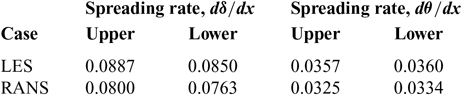
The spreading rate gives a quatitative measure of free shear layer development and can be calculated based on either the momentum thickness, Equation (8), or the physical width of the mixing layer between the y 0.90 and y 0.10 points, according to Equation (9). The points used to predict the spreading rate lie in the range of x/c = −0.2 to x/c = 70 which puts them roughly in the region of mixing layer approximate self-similarity in Fig. 1. The spreading rate data points are shown in Fig. 15 for LES(Reference Al-Shabab4) and the modified RANS model and the values are summarised in Table 3, these values lie comfortably within the spread of experimental measurements for equivalent cases of a single sided mixing layer available in the literature,(Reference Pope24).
 $$S{R_\theta } = {{d\theta } \over {dx}},\quad \quad \theta = \int_{ - \infty }^\infty {{U - {U_{{\rm{L}}ow}}} \over {{U_{{\rm{H}}igh}} - {U_{{\rm{L}}ow}}}}\left( {1 - {{U - {U_{{\rm{L}}ow}}} \over {{U_{{\rm{H}}igh}} - {U_{{\rm{L}}ow}}}}} \right)dy$$
 $$S{R_\delta } = {{{U_C}} \over {{U_S}}}{{d\delta } \over {dx}},\quad \quad \delta = {y_{0.90}} - {y_{0.10}}$$
 $$\begin{equation*}
\hspace{10pt} y_\alpha = U_{\rm Low} + \alpha \left( U_{\rm High} - U_{\rm Low} \right), \hspace{10pt} \hspace{10pt} U_C = \frac{1}{2} \left( U_{\rm High} + U_{\rm Low} \right), \hspace{10pt} \hspace{10pt} U_S = \left( U_{\rm High} - U_{\rm Low} \right)
\end{equation*}$$
Free Shear Layers Spreading Rate Values

Free shear layer spreading rate data.

Another interesting feature to explore, which is often ignored, is the location of the mixing layer’s virtual origin. The virtual origin is defined as the point of convergence of the lines fitted through 95%, 50% and 10% points of the velocity difference across the mixing layer at consecutive streamwise positions(24). These are often referred to as y 0.95, y 0.50 and y 0.10 lines.
Open jet with aerofoil virtual origin.

Figure 16 shows the estimated location of the virtual origin with the aerofoil installed in the working section. When the prediction of the virtual origin is based on points that lie upstream of the point at which the free shear layers get deflected by the aerofoil, both virtual origins lie at the vertical location corresponding to the nozzle exit tip, which is the free shear layer’s physical seeding point. However, when the estimates are based on points that lie downstream of the free shear layer deflection point, there is a vertical shift in the location of the virtual origin of the lower shear layer while the lines of the upper shear layer fail to converge to a single point. The influence of the aerofoil on the characteristics of the upper free shear layer’s virtual origin is illustrated schematically in Fig. 17, wherein the effect is exaggerated for clarity.
In the absence of convergence of the y 10, y 50 and y 95 to a single point there is some confusion regarding the definition of the virtual origin deflection. The approach adopted here is to use the maximum vertical deflection relative to the nozzle tip of all the separate lines intersection points. This helps emphasise the interaction and does not have any qualitative effect on the understanding of the data, in terms of the bias for stronger interaction with one shear layer over the other. Any consistent scheme of defining the vertical deflection, such as averaging the deflection of all the separate intersections, should convey the information about the interaction between the aerofoil and the free shear layers, but the bigger deltas help facilitate the interpretation of the results and the relative comparison. The development of the virtual origin deflection concept for open jet configuration design purposes is further formalised in Al-Shabab and Tucker(Reference Al-Shabab and Tucker25).
Schematic of virtual origin behaviour.

To ensure that the observed virtual origin behaviour is not merely a RANS modeling effect, the vertical deflection of the virtual origin is compared with the LES results as the points used to predict the position are successively shifted downstream. There is a clear increase in the deflection on moving downstream as the free shear layer gets deflected by the aerofoil, it is also evident that the interaction with the upper shear layer is considerably stronger than that with the lower one. RANS predicts the general trend of the lines successfully as well as the stronger interaction with the upper shear layer.
Free shear layer virtual origin vertical deflection.

To produce Fig. 18, a total of 50 points were used with a bin size of 21 points along the free shear layers for each virtual origin position prediction with a uniform spacing between successive points. The edge of the free shear layer was defined based on a vorticity magnitude limit.
As a further proof of concept, it is possible to compare the virtual origin position of an empty open jet wind tunnel with the results shown above when the aerofoil is loaded.
Empty wind tunnel virtual origin.

In an empty open jet, the lines of best fit through both groups of points, Fig. 19, converge towards a virtual origin that is located roughly at the nozzle exit lips. Obviously, the physical significance of the two groups is lost in the absence of an aerofoil, but this result confirms that the variations in virtual origin properties found earlier are indeed linked to the interaction with the aerofoil.
The observed variation in the free shear layer’s virtual origin characteristics reveals a few important features about the aerofoil’s influence on the free shear layers and the nature of their interaction:
• When the aerofoil deflects the free shear layer, the inner region is deflected more than the outer region. This results in the loss of convergence towards a single virtual origin of the mixing layer.
• The larger deflection of the inner mixing layer region has implications for the unsteady structures within it, as the deflection is not a solid body rotation but rather subjects these structures to strains that originate from the interaction process rather than mixing layer dynamics.
• Two characteristics of the virtual origin could be used as metrics for the interaction with the aerofoil; the first is the convergence, or lack thereof, towards a single virtual origin, and the second is the vertical deflection in the virtual origin location.
The appealing feature about the virtual origin behaviour is the possibility of its development into a design parameter that can facilitate fying the interaction level through, for example, monitoring the virtual origin’s vertical deflection in different configurations. Such an approach can be used to improve the placement of the aerofoil inside the working section for weaker overall interaction with the free shear layers. Focusing on the vertical deflection can also be viewed as a data reduction technique that can effectively convert the two-dimensional free-shear layer development field into a one-dimensional line or even a single value, if the maximum or an averaged deflection is used.
5.0 CONCLUSIONS
A RANS-based approach was adopted to predict open jet installations effects with focus on the aerospace oriented Menter SST model, where RANS results were validated against the available laboratory measurements and LES data. With the appropriate corrections implemented, the SST model performance was found to be promising, as most features of the interaction were captured. The notable exception was the background disturbance level in the potential core, which requires a hybrid LES-RANS approach that resolves the unsteady large scale structures in the free shear layers.
On the flow physics side, the mixing layer’s virtual origin was observed to exhibit strong sensitivity to the interaction with the aerofoil, which can be developed into a metric of the interaction between the aerofoil and the free shear layers, hence providing a quantitative design parameter to assist in the design of open jet experiments. The behaviour of the virtual origin observed in RANS simulations was validated against high-fidelity LES data confirming that it is a physical consequence of the interaction. Furthermore, the inner part of the free shear layers was found to suffer a greater deflection than the outer part, leading to the introduction of strains related to the interaction with the aerofoil rather than mixing layer dynamics. These two observations emphasise the impact of the interaction with the aerofoil on the mixing layer development, a point that has been largely ignored in previous studies.
Finally, as an overall view of the envisaged role for RANS-based simulations in open jet noise investigations, it must be emphasised that this role is complementary to experimental measurements and high fidelity simulations, such that these more expensive activities can become more effective. Given the relative inexperience in the application of RANS to open jet problems, some form of reference data either from a preliminary experimental run or a baseline high-fidelity simulation will be required to provide validation. However, once confidence in the RANS model is established, it provides an extended range of options for comparing different experimental configurations and optimising the setup. It might be possible to relax the requirement for case specific validation when the repository of open jet cases successfully modeled using RANS expands. This encourages further testing and focus on incorporating RANS-based interaction analysis into the design of open jet aerofoil experiments, particularly since the cost of RANS is a small fraction of the cost of a full LES (approximately 1/65,000 in this case).