TPM principle

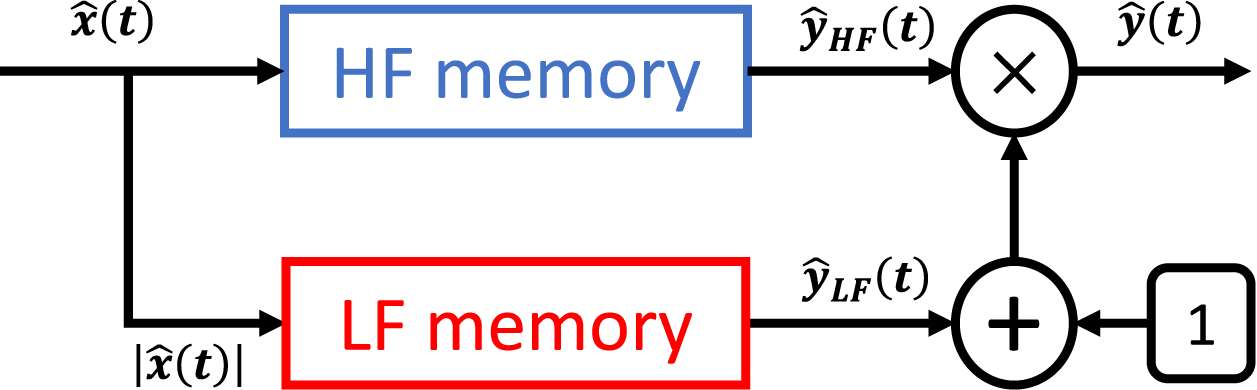
The TPM model is derived from Volterra series model simplifications [Reference Ngoya, Quindroit and Nébus6]; it is broadly based on a differentiated identification of nonlinear dynamics exhibiting short time constants to that exhibiting longer time constants. These are equivalently referred to as HF and LF memory effects. The HF memory effects grossly exhibit time constants in the order of the RF carrier period (e.g., due to RF group delay of transistor, frequency dispersions of filters and matching circuits, etc.), and conversely, LF memory effects exhibit time constants much higher, in the order of modulation signal speed (e.g., due to slow changes in transistor self-bias point, self-heating temperature conditions, electronic traps, etc.). The model block diagram is therefore as sketched in Fig. 1, where each memory path is represented by a different kernel.

Figure 1.

TPM model topology.

To identify the TPM model, it is necessary to perform two series of device characterizations, in the frequency domain, using elemental CW signals. The first series of characterization is carried out by driving the device with a single-tone non-modulated CW carrier signal, i.e., $x(t)=X_0.\text{cos}(2\pi.f_0.t)$; it allows to identify the HF kernel of PA.

Then, a second characterization is carried out driving the device with a low-index modulated CW carrier signal, i.e., $x(t)=X_0.\text{cos}(2\pi.f_0.t)+\delta X.\text{cos}(2\pi.(f_0+\delta f).t+\delta \varphi)$; it allows to identify the LF kernel, as described [Reference Gapillout, Mazière, Ngoya and Mons7]. The response of each path in the model (HF and LF paths) expresses a Hammerstein model convolution integral:

(1)\begin{equation} \hat{y}(t)=\hat{y}_{HF}(t).\left({1+\hat{y}_{LF}(t)}\right) \end{equation}

(2)\begin{equation} \hat{y}_{HF}(t)=\int_0^t h_{HF}(|{x(t-\tau})|,\tau).x(t-\tau)\; d\tau \end{equation}

(3)\begin{equation} \hat{y}_{LF}(t)=\int_0^t h_{LF}(|{x(t-\tau})|,\tau).x(t-\tau)\; d\tau \end{equation}

Extraction of the TPM model consists, from the above measurements, in identifying the frequency domain, the two transfer functions $H_{HF}(X_0,f)$ and $H_{LF}(X_0,f)$, corresponding respectively to Fourier transforms of the two time-domain kernels $h_{HF}(X_0,\tau)$ and $h_{LF}(X_0,\tau)$ in the above equations. To perform a complete characterization of the PA it is necessary to sweep the signal amplitude X ₀ over the entire power operating range of the PA, from the linear to saturation region. Similarly, the carrier frequency f ₀ as well as the modulation frequency $\delta f$ must be swept to cover operating bandwidth of the PA.

Fundamental limitation

As mentioned in the introduction, the TPM model has shown satisfactory modeling of RF PA response, regardless of the modulation signal used, both on narrowband and wideband applications. However, a structural limitation of TPM model arises from the fact that, as described above, the measurements necessary for model identification need to be carried out in the CW regime, from linear to saturation region. Indeed, in the case of high-power applications, self-heating of the PA can lead to its destruction in the saturation region. In the next section, we investigate the alternate approach based on PA characterization in the time domain, using pulsed RF excitation, offering the possibility for self-heating control by monitoring the pulse duration.

Principle of the NIR model

The principle of PA modeling on the basis of time-domain pulsed RF measurements has already been adopted in the past, in several works, under the designation Nonlinear Impulse Response (NIR) model [Reference Soury, Ngoya and Nébus8–Reference Verspecht, Horn, Betts, Gunyan, Pollard, Gillease and Root10]. In this work, we re-evaluate the NIR principle, to investigate to what extent it could be useful in solving the fundamental limitation of TPM model indicated above.

Considering both the envelopes $\hat{x}(t)$ and $\hat{y}(t)$ of the input and output signals to the PA, the simplest expression of NIR model is given by the convolution integral below:

(4)\begin{equation} \hat{y}(t)=\int_0^\infty h(|{\hat{x}(t-\tau})|,f_{\hat{x}}(t-\tau),\tau).\hat{x}(t-\tau)\; d\tau \end{equation}

(5)\begin{equation} f_{\hat{x}}(t)=\frac{d\varphi_{\hat{x}}(t)}{dt} \end{equation}

where $|\hat{x}(t)|$ and $f_{\hat{x}}(t)$ are time-varying magnitude and instantaneous frequency of the input envelope signal, and the kernel $h(|\hat{x}|,f_{\hat{x}},\tau)$ stands for the nonlinear impulse response of the device [Reference Roblin, Root, Verspecht, Ko and Teyssier4]. For the sake of simplicity, we may neglect dependence on instantaneous frequency and impulse response reduces to a two-dimensional kernel in (6).

(6)\begin{equation} \hat{y}(t)=\int_0^\infty h(|{\hat{x}(t-\tau})|,\tau).\hat{x}(t-\tau)\; d\tau \end{equation}

Construction of the non-linear impulse response model

PA characterization principle

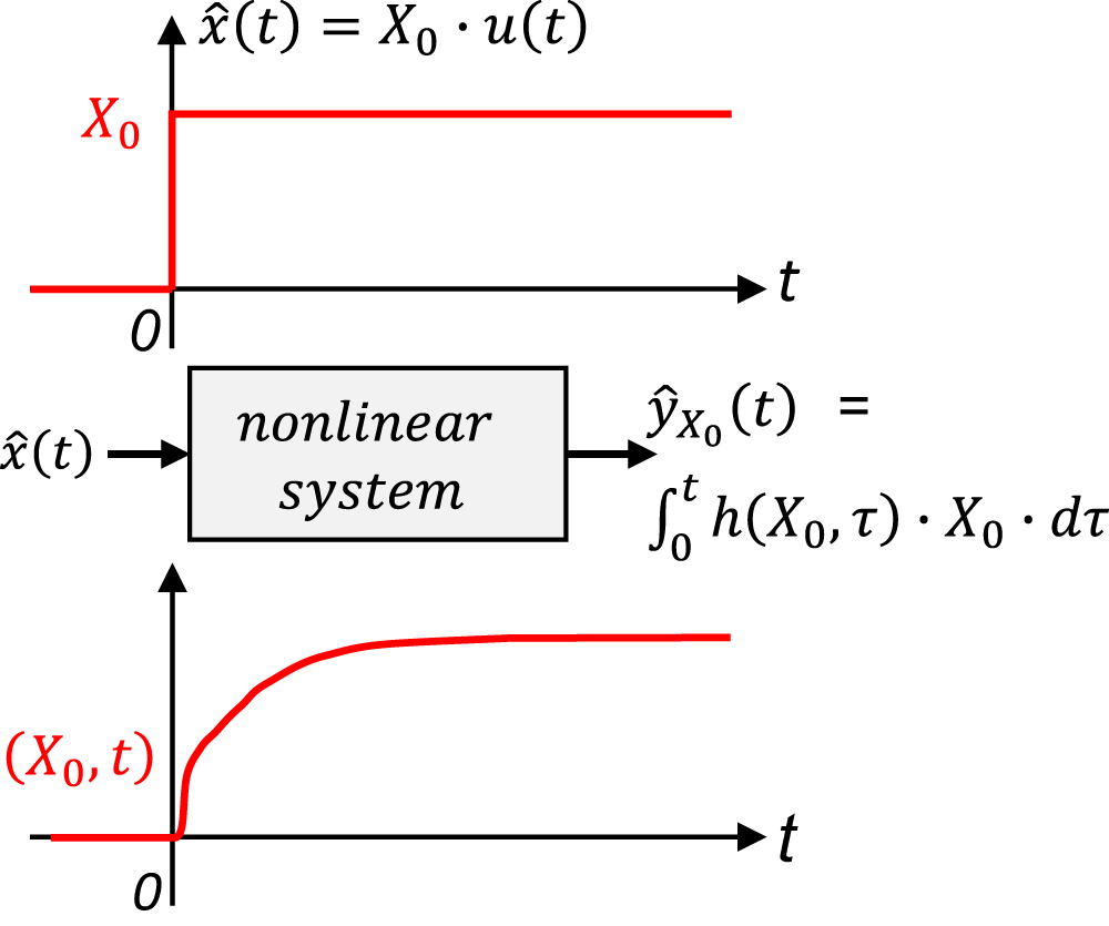
From the above equations, the optimal identification stimulus of the PA impulse response is easily determined as a unit time step function, as sketched in Fig. 2.

Figure 2.

Characterization stimulus for NIR model identification.

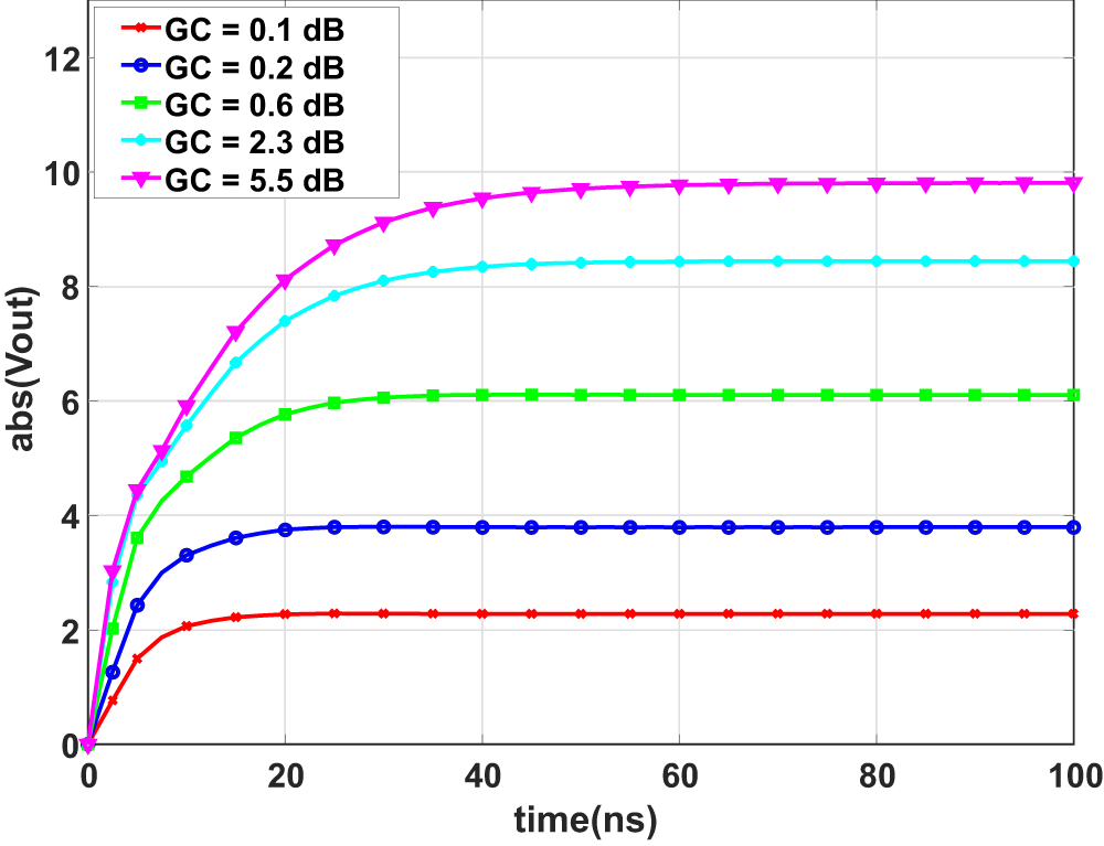
PA characterization for NIR model therefore requires driving the device with a series of unit step signals (RF pulses), $X_0.\text{cos}(2\pi.f_0.t).u(t)$. For complete characterization, amplitude X ₀ of the pulse is swept to cover the power operating range (linear to saturation region) of the PA. The corresponding step responses will then be used to identify the nonlinear impulse response. This type of characterization could be carried out in a measurement lab using an equipment like VST (Vector Signal Transceiver) incorporating a VSG (Vector Signal Generator) and a VSA (Vector Signal Analyzer) sharing the same local oscillator to ensure the phase coherence of the input-output signals. In this article focusing on the evaluation of theoretical principles, we will consider characterizing the PA only from the circuit simulation engine, using the circuit-envelope tool in the ADS simulator. For illustration purposes, we show in Fig. 3, the characteristics of a single-stage LDMOS PA, simulated with ADS circuit-envelope. We observe the step responses, for RF pulses applied at center frequency $f_0 = 830\, \text{MHz}$, of the PA. The four pulse amplitudes considered cover the PA operating region from 0.1 to 5.5 dB power Gain Compression (GC). We may observe from the time slopes of the step responses a shortest time-constant around 3 ns and a longest around 100 ns. It may be noted that, because the LDMOS transistor model did not consider electrothermal and trapping effects, the long-time-constant is only due to self-biasing effects.

Figure 3.

Pulse responses of LDMOS PA (ADS circuit-envelope) at $f_0 = 830\,\text{MHz}$.

Identifying the nonlinear impulse response

As defined in equation (6), the impulse response, $h(X_0,t)$, of the PA is a function with two variables, amplitude, and integration time, contained in the convolutional integral giving rise to step response of the PA. There are different methodologies for identifying impulse response $h(X_0,t)$ from the step response $Y(X_0,t)$. Optimal methodologies, minimizing the impact of inevitable measurement errors ensuring good numerical stability to the model, assume that response $Y(X_0,t)$ can be expanded into a series of separable basis functions in the dimensions X ₀ andt. Thus,

(7)\begin{equation} h(X_0,t)=\sum_{k=1}^K S_k.\alpha_k(X_0).\beta_k(t) \end{equation}

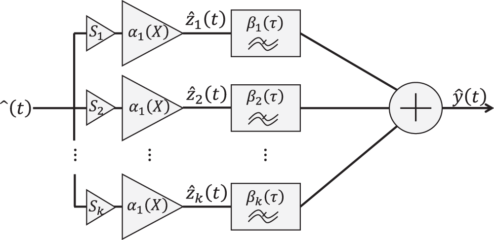
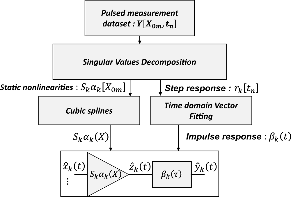
This formulation infers that the model can be represented by a set of parallel Hammerstein models, as shown in Fig. 4. Each branch consists of a static gain nonlinearity $S_k.\alpha_k(X_0)$, followed by a linear impulse response filter $\beta_k (t)$. This arrangement is particularly useful for implementing the model in simulation environments.

Figure 4.

NIR model topology.

From the above postulate, it follows that an optimal expansion (i.e., minimal expansion size and orthogonal basis functions α_k and β_k) can be obtained using the singular value decomposition (SVD) method, as described in [Reference Ngoya, Quindroit and Nébus6].

To do so, we form a two-dimensional matrix from database of the PA step responses $Y(X_{0m},t_n)$; $m = 1,\dots,M$; $n=0,\dots,N-1$, where M and N are respectively the numbers of step amplitudes and time samples. Applying SVD to the matrix we obtain the form

(8)\begin{equation} Y(X_0,t)=\sum_{k=1}^K S_k.\alpha_k(X_0).r_k(t) \end{equation}

where we readily identify that basis functions $r_k(t)$ in (8) are the step responses corresponding to the desired filter impulse responses $\beta_k(t)$ in (7), i.e.:

(9)\begin{equation} r_k(t)=\int_0^t \beta_k(\tau).u(t-\tau)\;d\tau \end{equation}

It is worth noticing that knowledge of the singular values of measurement database allows for an easy truncation of the series in (7), which will determine the number of parallel channels in Hammerstein model. In practice, a 60 dB relative threshold $S_K/S_1$ guaranties good accuracy to the model, while filtering out major measurement errors.

Interpolation of the basis functions

It is important to note that the set of basis functions $\alpha_k (X_0)$ and $\beta_k(t)$ obtained from the procedure, are known only at discrete points $X_{0m}$ and t_n of the two variables, corresponding to the set of measurement points. In order to use the model under arbitrary excitation conditions, it is necessary to interpolate the basis functions between the measurement points. For reasons of robustness, interpolation by cubic splines is usually recommended for static nonlinearities $\alpha_k(X_0)$. For the impulse response of the filters, $\beta_k(t)$, it is more appropriate to use rational function interpolation; the most popular and effective method being that Vector Fitting (VF) [Reference Gustavsen and Semlyen11], briefly recalled. VF method was initially developed for frequency domain identification of linear transfer functions in the form:

(10)\begin{equation} H(\Omega)=\sum_{n=1}^N \frac{C_n}{j\Omega-a_n}+d \end{equation}

It was later on extended to the direct time-domain identification of linear impulse response, as the Time-Domain Vector Fitting (TD-VF) method [Reference Grivet-Talocia12]. Thus, if we reconsider the pole relocation technique introduced in [Reference Gustavsen and Semlyen11] into (10),

(11)\begin{equation} \sum_{n=1}^N \frac{C_n}{j\Omega-\tilde a_n}+d=\left({\frac{\tilde C_n}{j\Omega-\tilde a_n}+d}\right).H(\Omega) \end{equation}

Where $\tilde C_n$ and $\tilde a_n$ are the relocated poles and residues of the original equation (10). Then considering from (10), that the transfer function $H(\Omega)$, is ratio of system output to input spectrum, $Y(\Omega)$ and $X(\Omega)$, we get:

(12)\begin{equation} \left({\sum_{n=1}^N \frac{C_n}{j\Omega-\tilde a_n}+d}\right).X(\Omega)=\left({\frac{\tilde C_n}{j\Omega-\tilde a_n}+d}\right).Y(\Omega) \end{equation}

Applying the inverse Laplace transform, we get the time formula of TD-VF below:

(13)\begin{equation} \sum_{n=1}^N C_n.x_n(t)+d.x(t)=y(t).\sum_{n=1}^N \tilde C_n.y_n(t) \end{equation}

Where

(14)\begin{equation} x_n(t)=\int_0^te^{\tilde a_n(t-\tau)}x(\tau)\;d \tau \end{equation}

(15)\begin{equation} y_n(t)=\int_0^te^{\tilde a_n(t-\tau)}y(\tau)\;d \tau \end{equation}

Finally, considering discrete integral over time in (14) and (15), we obtain a linear system equation that can be solved identically to the original frequency domain VF method [Reference Grivet-Talocia12]. As a summary, the different stages of NIR model identification and implementation are sketched in the block diagram below, Fig. 5.

Figure 5.

NIR model identification and implementation.

Applying the above NIR principles allows for PA modeling using pulsed RF signals. This open up possibility to overcome the problems for PA destruction by self-heating, through adjustment of pulse duration.

Evaluation of the NIR model

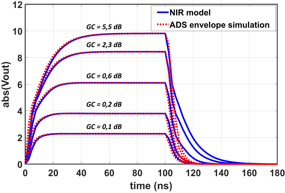
We have applied the above methodology to the LDMOS amplifier schematic indicated previously, and extracted the corresponding NIR model. The model evaluation results are shown in the figures below, for two different excitation conditions; RF pulse response test and frequency domain single-tone CW test. Figure 6 shows the response to the PA RF pulse excitation, where we have varied the pulse amplitude to cover 0–5 dB of gain compression range. The carrier frequency is located at PA bandwidth center frequency, 830 MHz. We compared the NIR model response with ADS circuit-envelope simulation. We may observe that the NIR model can reproduce accurately enough the rising front of the RF pulse response. However, it exhibits a large discrepancy on the falling edge, as the input amplitude grows into a gain compression region. This phenomenon is unfortunately a known characteristic of the Hammerstein model, identified as symmetry of the response [Reference Verspecht, Horn, Betts, Gunyan, Pollard, Gillease and Root10].

Figure 6.

Pulse response test – comparison: NIR model and ADS circuit-envelope simulation.

Figure 7.

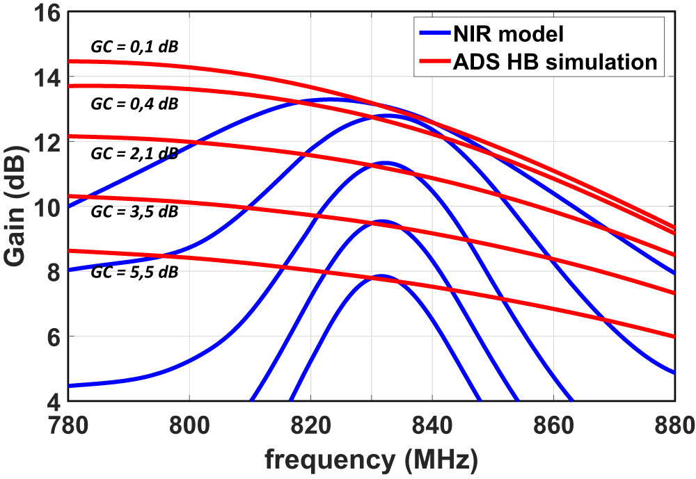
CW response test – comparison: NIR model and ADS HB simulation.

Figure 7 shows single-tone CW gain of the PA, with input power varied to cover a range from 0 dB to 5 dB of gain compression, over a frequency bandwidth of 100 MHz around 830 MHz center frequency. NIR model matches with ADS harmonic-balance (HB) simulation only at a very small vicinity of the center frequency. As we move from center, NIR model results are inconsistent.

A first-order analysis of the NIR model shows that the poor performance observed comes mainly from an intrinsic limitation of its characterization and identification principle. In fact, accuracy of the NIR model is intrinsically limited by the constraint on the pulse envelope sampling time step. Indeed, the sampling time step for observing the envelope signal cannot be less than half of the carrier period, because this would lead to spectrum aliasing between harmonics of the carrier frequency. In the present test case, the time step cannot be less than 2/830 MHz = 2.5 ns. This much large time step does not allow to effectively discriminate between HF (short-term memory) and LF (long-term memory) effects. Extensions of the NIR model have been proposed in an attempt to improve its performance [Reference Ngoya and Mons13]; the most relevant approach being the one proposed in [Reference Verspecht, Horn, Betts, Gunyan, Pollard, Gillease and Root10]. This proposes an identification of the core of the model on the basis of a series of two-level RF pulses, instead of single-level RF pulses we have used. A two-level pulse provides more information on the nonlinear transitions on rising and falling fronts, allowing us to overcome the response symmetry problem. However, this principle does not allow us to overcome the limitation due to the sampling step which impacts the model CW response. In addition, two-level pulse characterization introduces significant measurement complexity since the number of variables is increased from two to three (the two pulse levels and observation time). To conclude, we may nevertheless notice from the pulse response test, Fig. 6, that the long time-constants of the PA are rather well reproduced by the NIR model on the rising edge of the pulse. This is a good indication of NIR model’s ability to accurately capture LF memory effects of the PA. There in the next section, we consider a pragmatic solution to consider a combination of the NIR model with the original TPM model, where there is an explicit separation between the HF and LF memory effects. Thus, in this combination, the NIR model will be specialized to capture only LF memory effects, while HF memory effects continue to be characterized with conventional CW measurements, as described in Section 2.

TPM-NIR model principal

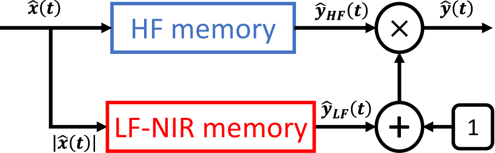
The combined TPM-NIR model has a structure identical to the original TPM model, Fig. 8, presented in Section 2. The only difference lies in the methodology for identification of the LF memory kernel. We will not delve into the principle for HF model kernel identification, which is extensively described in previous work [Reference Ngoya, Quindroit and Nébus6, Reference Ngoya and Mons13]. This is, similar to the above description of NIR principles, based on SVD decomposition, and two-way interpolation scheme (cubic splines for input amplitude and VF for CW frequency) of the CW measurement database.

Figure 8.

TPM-NIR model topology.

Output signal $\hat y_{LF}(t)$ of the LF-NIR path is expressed exactly as in equation (3) of the original TPM model, Section 2. In order to identify kernel of the LF-NIR path, it is essential to isolate the step response $\hat y_{LF}(t)$ resulting from its output, when the PA is excited by an RF pulse. To do this, we start by identifying the model of the HF path, as indicated in Section 2, using the CW characteristics. Then, in a second stage, we characterize the PA, as described in the previous section, using RF pulses. A simple analysis of the TPM-NIR block diagram shows that we can easily isolate the step response of LF memory path output as below:

(16)\begin{equation} \hat y(t)=\hat y_{HF}(t).\left({1+\hat y_{LF}(t)}\right) \end{equation}

(17)\begin{equation} \hat y_{LF}(t)=\frac{\hat y(t)}{\hat y_{HF}(t)}-1 \end{equation}

Knowing the model of HF memory path, we can then construct a corresponding measurement database as seen from the LF memory path output. Finally, we can reapply the methodology of previous section to identify kernel of the LF memory path.

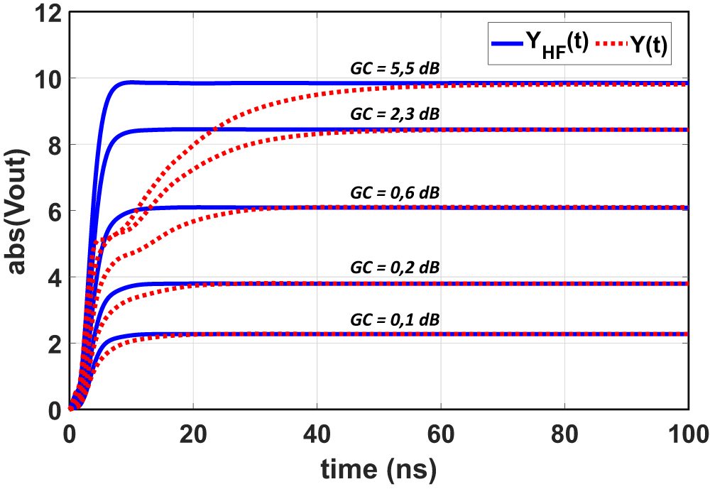
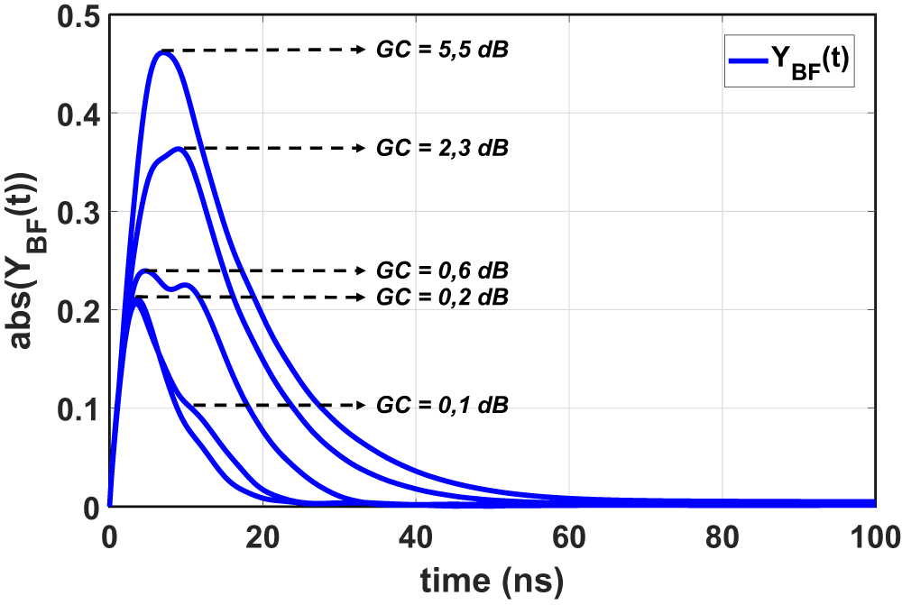
For illustration, we have applied the above process to the previous LDMOS PA circuit, from which we obtain the characteristics shown in Fig. 9 and Fig. 10. Figure 9 shows the superposition of total PA circuit step response and LF memory path step response, for various values of gain compression. Figure. 10 shows the corresponding step response as seen at the output of the LF memory path. We can then distinctly observe differences in time-constants between HF and LF memory paths.

Figure 9.

Total PA pulse response $\hat{y}(t)$, HF memory path pulse response $\hat{y}(t)$.

Figure 10.

LF memory path pulse response $\hat{y}_{LF}(t)$.

Evaluation of the TPM-NIR model

From the above methodology, we have extracted the TPM-NIR model of the PA. The kernel of each memory path has been represented by a parallel Hammerstein model. SVD expansion method allowed to select three parallel channels for each memory path. A convenient number of poles was found to be 3 for the HF kernel and 5 for the LF kernel. An evaluation of the model performance is given below for different excitation stimuli, with a comparison between the original TPM model, extended TPM-NIR model and ADS circuit simulations.

RF pulse response

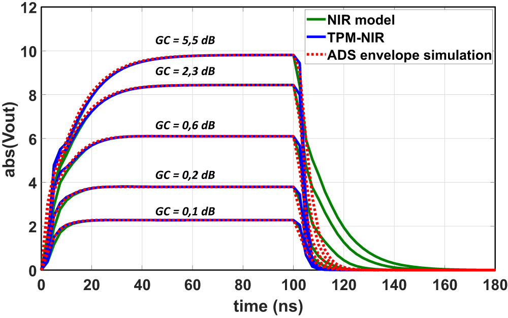
Figure 11 shows the comparison of the pulse responses of the NIR and TPM-NIR models with the circuit-envelope simulation, for varying gain compression level. A good TPM-NIR prediction can be observed on both rising and falling fronts of the pulse, all over gain compression range.

The response symmetry observed with the integral NIR model has been resolved. We may nevertheless notice a small mismatch with ADS circuit-envelope simulations on both fronts, which are rather attributed to an inaccuracy of the circuit-envelope simulation due to the limitation of envelope sampling time step already mentioned.

Figure 11.

Pulse response test – comparison: NIR, TPM-NIR model and ADS circuit-envelope simulation.

Single-tone CW response

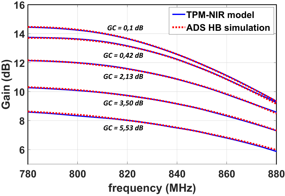
Figure 12 compares single-tone CW of the PA, from TPM, TPM-NIR model and ADS circuit simulation, for varying PA gain compression in 100 MHz bandwidth. We can observe a perfect agreement on these CW characteristics.

Figure 12.

CW response test – comparison: TPM-NIR model and ADS HB simulation.

Third-order intermodulation distortion (IMD3)

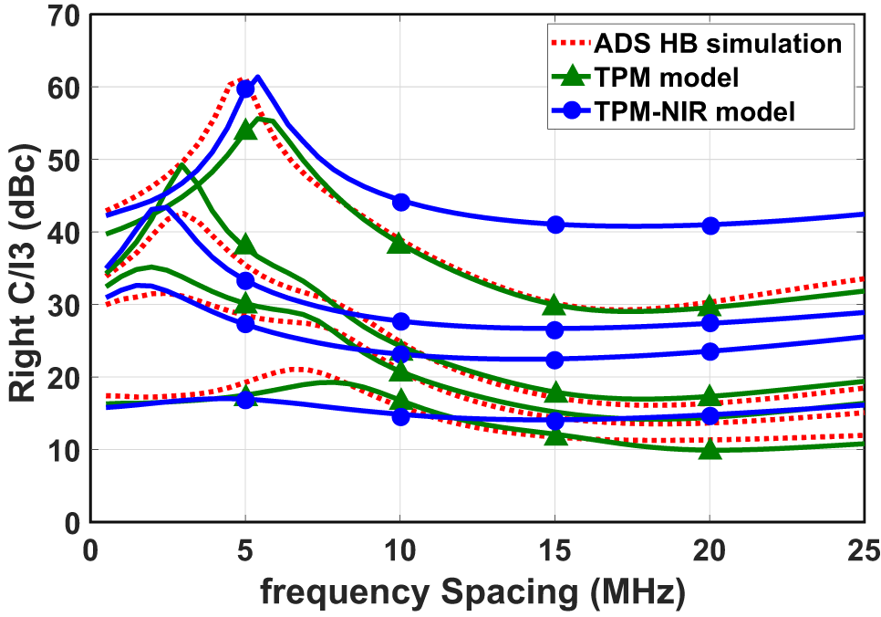
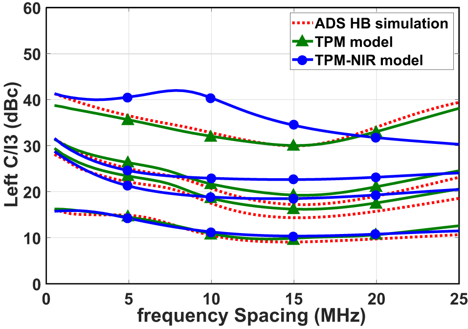
The PA has been simulated using an equal-amplitude two-tone excitation. The two tones are placed at an equal distance from the bandwidth center of 830 MHz. Ratios of IMD3 have been recorded for varying input tone power, from 0 to 5 dB gain compression, and two-tone distance from 1 to 25 MHz. The results are presented on Fig. 13 and Fig. 14, for the left and right carrier to IMD3 ratios (C/I3), respectively, with a comparison between original TPM, TPM-NIR model and ADS circuit simulation.

Figure 13.

Right C/I3 – comparison: TPM, TPM-NIR models and ADS simulation.

Large left and right IMD asymmetry as well as important resonances are observed on the characteristics, indicating the presence of strong LF memory effects in the PA.

The results of the TPM-NIR model, as well as the original TPM model, are not in perfect agreement with the ADS simulation, but the overall variation trend against tone distance and input power is obtained. It should be noted that two-tone IMD3 response, because of the resonance phenomena taking place, is the most difficult test to satisfy for a behavioral model, which in its globalizing concept aims to reproduce the average dynamics.

Figure 14.

Left C/I3 – comparison: TPM, TPM-NIR models and ADS simulation.

Modulated signal test

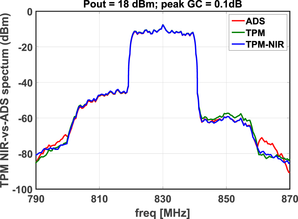
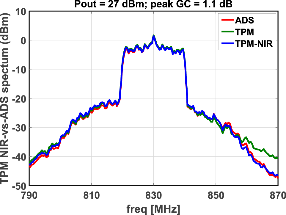
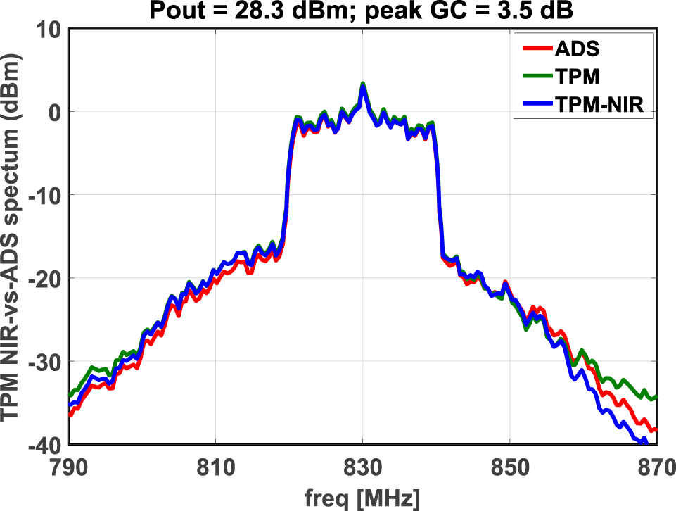
The last test concerns a 16-QAM modulation signal of 20 MHz bandwidth. In Fig. 15, Fig. 16 and Fig. 17, we present power spectrum of the output signal for 3 average power levels (Pin), corresponding to a peak gain compression level peak GC = 0.1 dB, 1.1 dB, 3.5 dB, respectively. The corresponding average output powers are also indicated in the figures. The figures compare the results of the two TPM models with the ADS simulation. As in the previous IMD3 figures, we observe a large left-to-right asymmetry of power spectral regrowth. The performance of the two TPM models is equivalent and in good agreement with the ADS simulation. Computational time comparisons between models and ADS simulation in a ratio greater than 100.

Figure 15.

Output power spectrum 16-QAM, $BW = 20\,\text{MHz}$, $P_{in} = 5\,\text{dBm}$.

Figure 16.

Output power spectrum 16-QAM, $BW = 20\,\text{MHz}$, $P_{in} = 16\,\text{dBm}$.

Figure 17.

Output power spectrum 16-QAM, $BW = 20\,\text{MHz}$, $P_{in} = 20\,\text{dBm}$.