2. GNSS POSITIONING ACCURACY OVERVIEW

The observed value in GNSS is range to satellite, measured on the basis of the difference between receiving and sending time of the navigation signal. Due to the fact that the value of the user's clock error is unknown the range is called pseudorange. The pseudorange measurement to a particular satellite can be described by the following observation equation (Parkinson and Spilker, Reference Parkinson and Spilker1996):

(1) $$\rho _i = R_i + c \cdot \delta T + \varepsilon _i = \sqrt {{\left( {x_{si} - x_u} \right)}^2 + {\left( {y_{si} - y_u} \right)}^2 + {\left( {z_{si} - z_u} \right)}^2} + c \cdot \delta T + \varepsilon _i\;, $$

where ρ _i is the measured pseudorange to the i-th satellite, R _i is the geometrical range to the i-th satellite, c is the mean speed of signal propagation, δT is the user's clock error and ε _i is the random measurement error, which is a composition of errors connected with ephemerids uncertainty, satellite clock error, ionospheric and tropospheric refraction, and noises of the user's receiver. x _si , y _si , z _si are the i-th satellite position in the Earth-Centred Earth-Fixed (ECEF) coordinates system and x _u , y _u , z _u is the user position in the ECEF coordinate system.

Satellite position is known at the time of measurement, because it can be calculated on the basis of data in the navigation message transmitted by the satellite. If it is additionally assumed that random measurement error can be modelled as an independent variable with zero-mean Gaussian distribution (N[0,1]) then Equation (1) will have four unknowns: user coordinates $\left( {x_u,\; y_u,z_u} \right)$ and value $\left( {c \cdot \delta T} \right)$ which is called metre equivalent of the user's receiver clock error. Therefore, pseudorange measurement to at least four satellites is necessary to fix the user's position. This is the first and fundamental condition of GNSS positioning availability. The second is connected with desired accuracy, which can be estimated as (Parkinson and Spilker, Reference Parkinson and Spilker1996):

(2) $$M = \sigma _p \cdot DOP$$

where M is the user's position mean error, σ _p is the root mean square of pseudorange measurements, depending on random errors $\left( \varepsilon \right)$ . For typical code receivers it is on the level of single metres and DOP is the coefficient of Dilution of Precision, depending on the satellite geometry (satellites location in relation to the user's position).

DOP coefficients can be calculated on the basis of a geometric matrix. Equation (1) is non-linear and to solve it, linearization is necessary. Usually Taylor's method is applied which is based on a priori information about the user's location. After linearization, Equation (1) takes the following form:

(3) $$\rho _i - R_{0i} = \displaystyle{{ - \left( {x_{si} - x_{0u}} \right)} \over {R_{0i}}} \cdot \Delta x + \displaystyle{{ - \left( {y_{si} - y_{0u}} \right)} \over {R_{0i}}} \cdot \Delta x + \displaystyle{{ - \left( {z_{si} - z_{0u}} \right)} \over {R_{0i}}} \cdot \Delta z + c \cdot \delta T$$

where x _0u , y _0u , z _0u are the a priori assumed user coordinates, Δx, Δy, Δz are the differences between true and a priori assumed user coordinates and R _0i is geometrical range from the a priori assumed user coordinates to i-th satellite:

(4) $$R_0 = \sqrt {{\left( {x_{si} - x_{0u}} \right)}^2 + {\left( {y_{si} - y_{0u}} \right)}^2 + {\left( {z_{si} - z_{0u}} \right)}^2} $$

All observation Equations (3) which describe performed pseudorange measurements to n visible satellites create the following matrix equation system:

(5) $$\left[ {\matrix{ {\rho _1 - R_{01}} \cr {\rho _2 - R_{02}} \cr {\matrix{ \hfill\vdots\hfill \cr {\rho _n - R_{0n}} \cr}} \cr}} \right] = \left[ {\matrix{ { - u_{x1}} & { - u_{y1}} & {\matrix{ { - u_{z1}} & 1 \cr}} \cr { - u_{x2}} & { - u_{y2}} & {\matrix{ { - u_{z2}} & 1 \cr}} \cr {\matrix{ \; \cr { - u_{xn}} \cr}} & {\matrix{ \vdots \cr { - u_{yn}} \cr}} & {\matrix{ {\matrix{ \; & \; \cr}} \cr {\matrix{ { - u_{zn}} & 1 \cr}} \cr}} \cr}} \right] \cdot \left[ {\matrix{ {\Delta x} \cr {\Delta y} \cr {\matrix{ {\Delta z} \cr {c \cdot \delta T} \cr}} \cr}} \right]$$

(6) $$\mathop {\Delta {\bf \rho } = {\bf G} \cdot \Delta {\bf X}\comma}\limits^ {\Downarrow} $$

where:

(7) $$u_{xi} = \displaystyle{{x_{si} - x_{0u}} \over {R_{0i}}},\; \; u_{yi} = \displaystyle{{y_{si} - y_{0u}} \over {R_{0i}}},\; \; u_{zi} = \displaystyle{{z_{si} - z_{0u}} \over {R_{0i}}}\; \; $$

The Matrix ${\bf G}$ in Equation (6) is mentioned before the geometric matrix. Equation (6) is over-determined in case of more than four measurements. The solution using the least-square-adjustment is given by:

(8) $$\Delta \hat{\bf X} = \left( {{\bf G}^{\rm T}{\bf G}} \right)^{ - 1}{\bf G}^{\rm T}\Delta {\bf \rho} \;. $$

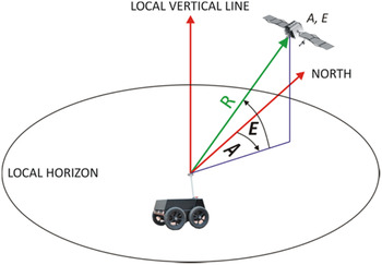
Expression $\left( {{\bf G}^{\rm T}{\bf G}} \right)^{ - 1}$ is the covariance matrix in the ECEF coordinates system. To compute DOP coefficients in the horizontal coordinates system, ${\bf G}$ has to be transformed to the East-North-Up (ENU) coordinates system (see Figure 1). After transformation we obtain:

(9) $${\bf G}_{{\rm ENU}} = \left[ {\matrix{ {cos\left( {E_1} \right) \cdot sin\left( {A_1} \right)} & {cos\left( {E_1} \right) \cdot cos\left( {A_1} \right)} & {\matrix{ {sin\left( {E_1} \right)} & 1 \cr}} \cr {cos\left( {E_2} \right) \cdot sin\left( {A_2} \right)} & {cos\left( {E_2} \right) \cdot cos\left( {A_2} \right)} & {\matrix{ {sin\left( {E_2} \right)} & 1 \cr}} \cr {\matrix{ \cr {cos\left( {E_n} \right) \cdot sin\left( {A_n} \right)} \cr}} & {\matrix{ \vdots \cr {cos\left( {E_n} \right) \cdot cos\left( {A_n} \right)} \cr}} & {\matrix{ { \matrix{ \; & \; \cr}} \cr {\matrix{ {sin\left( {E_n} \right)} & 1 \cr}} \cr}} \cr}} \right]$$

where E _i is the elevation of the i-th satellite and A _i is the azimuth of the i-th satellite.

Figure 1.

Azimuth and elevation of visible satellite.

As a result we obtain:

(10) $$\eqalign{{\bf C}_{{\bf X} \; {\rm ENU}} & = \left( {{\bf G}_{{\rm ENU}}^{\rm T} {\bf G}_{{\rm ENU}}} \right)^{ - 1} \cr & = \left[ {\matrix{ {V\left( E \right)} & {cov\left( {E,N} \right)} & {cov\left( {E,U} \right)} & {cov\left( {E,c \cdot \delta T} \right)} \cr {cov\left( {N,E} \right)} & {V\left( N \right)} & {cov\left( {N,U} \right)} & {\; cov\left( {N,c \cdot \delta T} \right)} \cr {cov\left( {U,E} \right)} & {cov\left( {U,N} \right)} & {V\left( U \right)} & {\; cov\left( {U,c \cdot \delta T} \right)} \cr {cov\left( {c \cdot \delta T,E} \right)} & {cov\left( {c \cdot \delta T,N} \right)} & {cov\left( {c \cdot \delta T,U} \right)} & {V\left( {c \cdot \delta T} \right)} \cr}} \right]}$$

and DOP can be calculated as follows:

(11) $${\rm global:}\quad GDOP = \sqrt {V\left( E \right) + V\left( N \right) + V\left( U \right) + V\left( {c \cdot \delta T} \right)} $$

(12) $${\rm position:}\quad PDOP = \sqrt {V\left( E \right) + V\left( N \right) + V\left( U \right)} $$

(13) $${\rm horizontal:}\quad HDOP = \sqrt {V\left( E \right) + V\left( N \right)} $$

(14) $${\rm vertical:}\quad VDOP = \sqrt {V\left( U \right)}$$

(15) $${\rm time:}\quad TDOP = \sqrt {V\left( {c \cdot \delta T} \right)} $$

Equation (2) shows that a lower value of DOP implies higher accuracy, so the most desired situation (from the autonomous precise navigation point of view) is when DOP values are as low as possible along the whole vehicle route. In order to achieve this, it is essential to compute which satellites will be visible and what values of azimuths and elevations will be like.

3. SATELLITE VISIBILITY

As a part of our research the following methodology of computation of satellites' visibility is proposed. Let us define the following matrices:

Satellites' visibility matrix $\left( {{\bf S}_{{\rm VS}}} \right)$ :

(16) $${\bf S}_{{\rm VS}} = \left[ {\matrix{ {SV_1} & {Health_1} & {Visible_1} \cr {SV_2} & {Health_2} & {Visible_2} \cr & \vdots &\cr SV_k& Health_k &{Visible_k}\cr}} \right]$$

where SV _i is i-th satellite identification number, Health _i is the i-th satellite health flag (true if satellite status is healthy, false if not), Visible _i is the i-th satellite visibility flag (true if satellite is visible, false if not) and k is the total number of satellites in constellations of all analysed systems.

Satellites' azimuths and elevations matrix $\left( {{\bf S}_{{\rm AE}}} \right)$ :

(17) $${\bf S}_{{\rm AE}} = \left[\matrix{SV_1 &A_{S1} &E_{S1}\cr SV_2 &A_{S2} &E_{S2}\cr &\vdots &\cr SV_k &A_{Sk} &E_{Sk}}\right]$$

where A _Si , E _Si are the azimuth and elevation of i-th satellite (in relation to the vehicle location).

Terrain profile matrix $\left( {{\bf T}_{{\rm AE}}} \right)$ :

(18) $${\bf T}_{{\rm AE}} = \left[ {\; \matrix{ {\matrix{ {A_{T1}} & {E_{T1}} \cr}} \cr {\matrix{ {A_{T2}} & {E_{T2}} \cr}} \cr {\matrix{ \vdots \cr {\matrix{ {A_{Tl}} & {E_{Tl}} \cr}} \cr}} \cr}} \right]$$

where E _Ti , A _Ti are the azimuth and maximum elevation of i-th terrain profile (in relation to the vehicle location) and l is the number of analysed terrain profiles.

Now we can claim the following:

(19) $${\bf S}_{{\rm VS}}\left( t \right) = f\left( {{\rm \;} {\bf S}_{{\rm AE}}\left( t \right),{\bf T}_{{\rm AE}}\left( t \right),t} \right)$$

where t is the moment of observation.

The ${\bf S}_{{\rm AE}} \; $ matrix is dependent on orbit parameters of the individual satellite and the vehicle location:

(20) $${\bf S}_{{\rm AE}}\left( t \right) = f\left( {{\bf O}_{\rm K}\left( t \right),{\bf V}_{\rm L}\left( t \right),t} \right)$$

where ${\bf O}_{\rm K}\left( t \right)$ is the Kepler's orbit parameters matrix for t and ${\bf V}_{\rm L}\left( t \right)$ is the vehicle location matrix for t, wherein:

(21) $${\bf O}_{\rm K} = \left[ {\matrix{ {SV_1} & {a_1} & {e_1} & {i_1} & {{\rm \Omega} _1} & {{ \dot {\rm \Omega}} _1} & {\omega _1} & {\mu _{01}} & {t_{oe1}} \cr {SV_2} & {a_2} & {e_2} & {i_2} & {{\rm \Omega} _2} & {{ \dot {\rm \Omega}} _2} & {\omega _2} & {\mu _{02}} & {t_{oe2}} \cr {} & {} & {} & {} & \vdots & {} & {} & {} & {} \cr {SV_j} & {a_j} & {e_j} & {i_j} & {{\rm \Omega} _j} & {{ \dot {\rm \Omega}} _j} & {\omega _j} & {\mu _{0j}} & {t_{oej}} \cr}} \right]$$

where a _i is the big semi-axis of i-th satellite orbit, e _i is the eccentricity of i-th satellite orbit, i _i is the inclination of i-th satellite orbit, Ω _i is the Right Ascension of the Ascending Node (RAAN) of i-th satellite orbit, $ \dot {\rm \Omega} _i$ is the rate of RAAN of i-th satellite orbit, ω _i is the argument of perygeum of i-th satellite orbit, μ _0i is the mean anomaly for t _oe of i-th satellite orbit, t _oei is the time of ephemeris of i-th satellite and

(22) $${\bf V}_{\rm L} = \left[ {\matrix{ {\varphi _V} & {\lambda _V} & {h_V} \cr}} \right]^{\rm T}$$

where ϕ _V , λ _V , h _V are the latitude, longitude and ellipsoidal height of the vehicle location. It is assumed that the reference surface for all computations is the WGS-84 ellipsoid.

After azimuths and elevations of all satellites have been computed, matrix $\left( {{\bf S}_{{\rm AE}}} \right)$ can be simplified to matrix $( {{\bf S}_{{\rm AE}}^{{\prime}}})$ the elements of which are only $\left( {SV_i,A_{Si},\; E_{Si}} \right)$ of satellites above the horizon:

(23) $${\bf S}_{{\rm AE}}^{{\prime}} = \left[\matrix{SV_1 &A_{S1} &E_{S1}\cr SV_2 & A_{S2} &E_{S2}\cr &\vdots &\cr SV_{k^\prime} &A_{Sk^{\prime}} &E_{Sk^{\prime}}}\right]$$

where k′ is the total number of satellites above the horizon.

The ${\bf T}_{{\bf AE}} \; $ matrix is dependent on terrain shape (approximated by DTM) and the vehicle location:

(24) $${\bf T}_{{\rm AE}}\left( t \right) = f\left( {{\bf T}_{{\rm DTM}},\; {\bf V}_{\rm L}\left( t \right),t} \right)$$

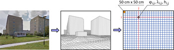
From a computational simplicity point of view it is assumed that the DTM model is a rectangular grid (cell dimension: 0·5 m x 0·5 m) where each node has an assigned latitude, longitude and ellipsoidal height (see Figure 2), thus:

(25) $${\bf T}_{{\rm DTM}} = \left[ {\matrix{ {{\bf T}_{{\rm P}1,1}} & {{\bf T}_{{\rm P}1,2}} & {\matrix{ \ldots & {{\bf T}_{{\rm P}1,q}} \cr}} \cr {{\bf T}_{{\rm P}2,1}} & {{\bf T}_{{\rm P}2,2}} & {\matrix{ \ldots & {{\bf T}_{{\rm P}2,q}} \cr}} \cr {\matrix{ \cr {{\bf T}_{{\rm P}p,1}} \cr}} & {\matrix{ \vdots \cr {{\bf T}_{{\rm P}p,2}} \cr}} & {\matrix{ { \matrix{ \; & \; \cr}} \cr {\matrix{ \ldots & {{\bf T}_{{\rm P}p,q}} \cr}} \cr}} \cr}} \right]$$

where:

(26) $${\bf T}_{{\rm Pi},{\rm j}} = \left[ {\matrix{ {\varphi _{i,j}} & {\lambda _{i,j}} & {h_{i,j}} \cr}} \right]^{\rm T}$$

and p is the dimension of modelled area in northern direction in metres × 2 and q is the dimension of modelled area in eastern direction in metres × 2.

Figure 2.

Process of DTM building.

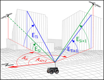
Using DTM it is possible to compute a terrain profile matrix $\left( {{\bf T}_{{\bf AE}}} \right)$ . To make computations simpler and faster in the proposed method only profiles on azimuths equal to the azimuths of satellites above the horizon are analysed (as shown in Figure 3). Thus the terrain profile matrix $\left( {{\bf T}_{{\rm AE}}} \right)$ can be written in the following form:

(27) $${\bf T}_{{\rm AE}} = \left[ {\; \matrix{ {\matrix{ {A_{S1}} & {E_{T1}} \cr}} \cr {\matrix{ {A_{S2}} & {E_{T2}} \cr}} \cr {\matrix{ \vdots \cr {\matrix{ {A_{S{k}^{\prime}}} & {E_{T{k}^{\prime}}} \cr}} \cr}} \cr}} \right]$$

Now visibility of the individual satellite can be defined in the form of the very simple condition:

(28) $$if\; E_{Si}\left( {A_{Si}} \right) \gt E_{Ti}\left( {A_{Si}} \right)\; then\; \; Visible_i = {\rm TRUE\;} else{\rm \;} Visible_i = FALSE $$

The above condition is illustrated in Figure 3.

Figure 3.

Relation between satellites' elevations $\left( {E_{Si}} \right)$ and maximum elevations of terrain profiles $\left( {E_{Ti}} \right)$ .

4. NUMERICAL EXPERIMENT

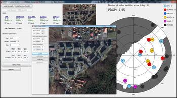
As a part of this research, numerical simulation of a small autonomous vehicle mission in the urban environment was performed. Copyrighted software by Aleksander Nowak (the paper's author) was used in the simulations. The software allows loading a DTM and planning the vehicle's route by giving waypoints and the vehicle speed between them. The waypoints can be pointed to directly on the map, input manually via dialogue window or be imported from a text file. The user has the ability to select which navigation satellite systems are used to perform a simulation (GPS, GLONASS, Galileo, BeiDou and additionally SBAS). The current orbit parameters of the systems are imported from almanac files. The user can also choose the start date and time of the simulation. As a result, text files including the satellite visibility and DOP values for points along the route with the desired resolution (standard resolution equals 1 m) are exported by the software. Moreover, the software computes the system availability on the basis of the predefined maximum DOP threshold. The main window of the software is presented in Figure 4.

Figure 4.

The main window of the built software.

4.1. Simulated urban environment

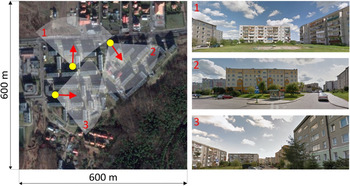
The simulated area was within one of the districts in the city of Gdynia, Poland. Its dimensions are 600 m x 600 m. Building density of this place is average and they are mostly five floors high. This is typical for small towns in Poland. The buildings there do not create urban canyons which can be observed in big cities, so at first glance there should not be many problems with GNSS positioning. Three examples of street views typical for this area are shown in Figure 5.

Figure 5.

The simulated urban environment (pictures from Google Maps).

The DTM model of the simulated urban environment was built on the basis of a point cloud from airborne laser scanning. The methodology of DTM building proposed for dynamic GNSS mission planning purposes will be described in another paper, but it should be emphasised here that the required accuracy of DTM is not as high in the case of GNSS mission planning as required in surveying tasks like inventory or cartography. Horizontal and vertical resolution equalling 0·5 m is sufficient. Moreover, it is not necessary to model every detail of terrain and buildings because the most important factor is elevation mask caused by obstructions created by both man-made and natural features of the urban environment. Therefore, the algorithm of the point clouds to DTM transformation is much simpler.

4.2. The vehicle and simulated route

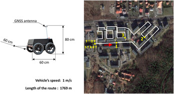
The simulations were performed for a small autonomous Unmanned Ground Vehicle (UGV). Its dimensions are presented in Figure 6. It is assumed that the vehicle goes along the planned route (shown in Figure 6) at constant speed of 1 m/s. The antenna of the GNSS receiver is mounted on the mast 0·8 m above the ground level.

Figure 6.

The UGV and its simulated route in the urban environment.

The dead reckoning process for simulation purposes was done on the basis of basic formulae:

(29) $$\eqalign{& \varphi _V\left( {t + \Delta t} \right) = \varphi _V\left( t \right) + \Delta \varphi _V\; \cr & \lambda _V\left( {t + \Delta t} \right) = \lambda _V\left( t \right) + \Delta \lambda _V\;} $$

where:

(30) $$\eqalign{& \Delta \varphi _V = V_V \cdot \Delta t \cdot cos\left( {H_d} \right) \cdot p_\varphi \; \cr & \Delta \lambda _V = V_V \cdot \Delta t \cdot sin\left( {H_d} \right) \cdot p_\lambda} $$

and V _V is the vehicle speed in $\left[ {{\raise0.7ex\hbox{${\rm m}$} \!\mathord{\left/ {\vphantom {{\rm m} {\rm s}}}\right.\kern-\nulldelimiterspace} \!\lower0.7ex\hbox{${\rm s}$}}} \right]$ , H _d is the vehicle heading (course) in [°], Δt is the time interval in [s], p _ϕ is the transition coefficient from metres to degrees for latitude $\left[ {{\raise0.7ex\hbox{$^\circ $} \!\mathord{\left/ {\vphantom {^\circ {\rm m}}}\right.\kern-\nulldelimiterspace} \!\lower0.7ex\hbox{${\rm m}$}}} \right]$ , p _λ is the transition coefficient from metres to degrees for longitude $\left[ {{\raise0.7ex\hbox{$^\circ $} \!\mathord{\left/ {\vphantom {^\circ {\rm m}}}\right.\kern-\nulldelimiterspace} \!\lower0.7ex\hbox{${\rm m}$}}} \right]$ , wherein:

(31) $$\eqalign{& p_\varphi = \left[ {1852 \cdot 60} \right]^{ - 1}, \cr & p_\lambda = \left[ {1852 \cdot 60 \cdot cos\left( {\varphi _V\left( t \right) + 0\cdot5\Delta \varphi _V} \right)} \right]^{ - 1}} $$

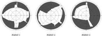
The horizon masks caused by the terrain obstacles for chosen points shown in Figure 6 (points 1, 2, 3) are presented in Figure 7.

Figure 7.

The horizon masks caused by the features of the modeled urban environment for points 1, 2, 3 shown in Figure 3 (print screens from the author's software).

4.4. Results of the experiment

In order to ensure clarity of the paper and due to the limited volume of the article, only selected and representative results of the numerical experiments are presented.

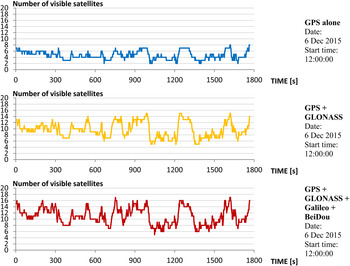
It is obvious that a multi-system GNSS receiver allows tracking of more satellites, even in urban environments. In Figure 8 it is shown how a significant increase of GNSS positioning quality is achieved when multiple constellations are used. As an example, the number of visible satellites distributed along the route for chosen UGV mission start time is illustrated.

Figure 8.

The number of visible satellites distributed along the route for different configurations of the satellite navigation systems.

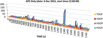
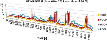
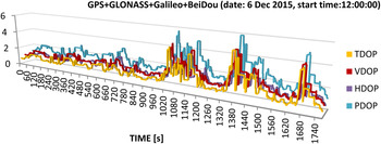
Of course, more observed satellites results in lower DOP values. Figures 9–11 show the DOP distribution along the route for the same UGV mission start time as in the case of Figure 8.

Figure 9.

The DOPs distribution along the route for GPS positioning.

Figure 10.

The DOPs distribution along the route for GPS + GLONASS positioning.

Figure 11.

The DOPs distribution along the route for GPS + GLONASS + Galileo + BeiDou positioning.

It can be seen that even with a relatively small density of buildings in the modelled urban environment, GPS alone is not sufficient to ensure reliable navigation. A combination of GPS + GLONASS gives much better GNSS performance, but still we have some sections of the vehicle route where PDOP is higher than 6. Additional satellites from Galileo and BeiDou keep PDOP values below level 6. It can be noticed that in the case of GPS alone positioning, a peak on the Horizontal Dilution of Precision (HDOP) chart has appeared and in consequence, it is also visible on the PDOP chart. Buildings cause signals from lower satellites (with low elevations) to be blocked and in consequence visible satellites create unfavourable geometry for the precise fix of horizontal coordinates. Multi-constellation receivers largely compensate this adverse effect.

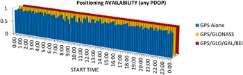
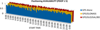
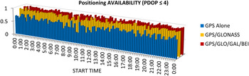
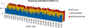
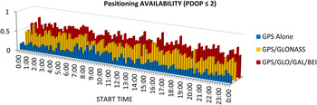
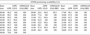
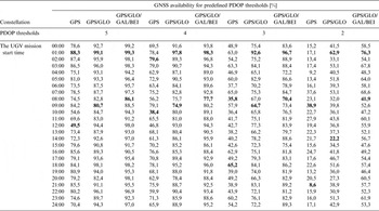
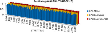
Figures 12–16 present the GNSS positioning availability as a function of the UGV mission start time, using GNSS systems and predefined maximum PDOP thresholds. Figure 12 presents the positioning availability for any PDOP value, which means that if four satellites were visible, the system was considered to be available. Subsequent figures show the increasing requirements for accuracy (lower admissible maximum PDOP values). The presented graphs clearly show that the GNSS positioning availability for a desired accuracy level depends not only on how many navigation satellites systems are used but also on the UGV mission start time. In other words, there are better and worse time windows to complete the task in the urban environment if the navigation process is based on GNSS. The same simulation results are presented in tabular form in Tables 1–3.

Figure 12.

The GNSS positioning availability for no predefined maximum PDOP threshold, as a function of the UGV mission start time and used GNSS systems (date: 6 Dec 2015).

Figure 13.

The GNSS positioning availability for predefined maximum PDOP threshold equals 5, as a function of the UGV mission start time and used GNSS systems (date: 6 Dec 2015).

Figure 14.

The GNSS positioning availability for predefined maximum PDOP threshold equals 4, as a function of the UGV mission start time and used GNSS systems (date: 6 Dec 2015).

Figure 15.

The GNSS positioning availability for predefined maximum PDOP threshold equals 3, as a function of the UGV mission start time and used GNSS systems (date: 6 Dec 2015).

Figure 16.

The GNSS positioning availability for predefined maximum PDOP threshold equals 2, as a function of the UGV mission start time and used GNSS systems (date: 6 Dec 2015).

Table 1.

The GNSS positioning availability as a function of the UGV mission start time, used GNSS systems and no predefined maximum PDOP threshold (date: 6 Dec 2015).

Table 2.

The GNSS positioning availability as a function of the UGV mission start time, used GNSS systems and predefined maximum PDOP threshold (date: 6 Dec 2015).

Table 3.

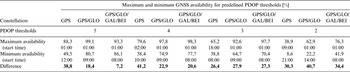
Maximum and minimum GNSS availability as a function of used GNSS systems and predefined maximum PDOP threshold (date: Dec. 6, 2015).

Some types of UGV mission do not require information about height. Due to the fact that the UGV's height above ground level is constant and equals 0, sometimes only horizontal coordinates are taken into account. In such cases, to assess quality of the GNSS positioning during the UGV mission, two states of the system can be defined as:

1. 1. Working State – current HDOP value is not higher than the predetermined maximum HDOP threshold.

2. 2. Failure State – current HDOP value is higher than the predetermined maximum HDOP threshold or number of visible satellites is insufficient to fix the position (fewer than four).

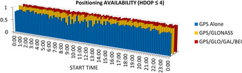
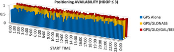
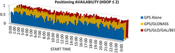
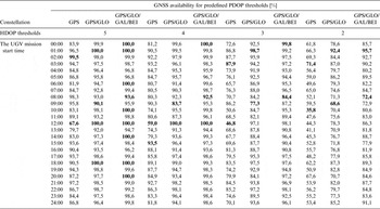
Figures 17–20 and Table 4 present the GNSS availability as a function of the UGV mission start time, used GNSS systems and predefined maximum HDOP thresholds.

Figure 17.

The GNSS positioning availability for predefined maximum HDOP threshold equals 5, as a function of the UGV mission start time and used GNSS systems (date: 6 Dec 2015).

Figure 18.

The GNSS positioning availability for predefined maximum HDOP threshold equals 4, as a function of the UGV mission start time and used GNSS systems (date: 6 Dec 2015)

Figure 19.

The GNSS positioning availability for predefined maximum HDOP threshold equals 3, as a function of the UGV mission start time and used GNSS systems (date: 6 Dec 2015).

Figure 20.

The GNSS positioning availability for predefined maximum HDOP threshold equals 2, as a function of the UGV mission start time and used GNSS systems (date: 6 Dec 2015).

Table 4.

The GNSS positioning availability as a function of the UGV mission start time, used GNSS systems and predefined maximum HDOP threshold (date: 6 Dec 2015).

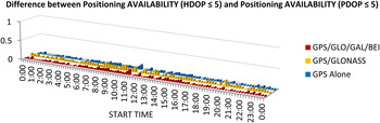
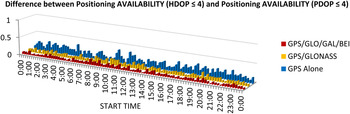
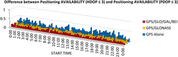
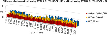
In Table 4 the emboldened values represent maximum and minimum GNSS positioning availability for the specified system configuration and predefined HDOP. It can be seen that the differences in the positioning availability are smaller if HDOP is taken into account instead of PDOP but are still significant in the case of GPS-only positioning (from 31·9% to 41,1%). Moreover, the differences grow with the increase of the accuracy requirements (with one exception in the case of GPS-only positioning). If maximum HDOP threshold is set at 2, the difference reaches 23·3% even if a multi-constellation receiver is used. It proves again that dynamic GNSS mission planning is necessary in order to ensure reliable navigation for the UGV even if only the horizontal accuracy is taken into account. In order to show how GNSS positioning availability increases when only horizontal coordinates are taken into consideration, differences between GNSS availabilities for predefined maximum HDOP and PDOP thresholds are shown in Figures 21–24.

Figure 21.

The difference between GNSS positioning availability for predefined maximum HDOP and PDOP thresholds equal 5 as a function of the UGV mission start time and used GNSS systems (date: 6 Dec 2015).

Figure 22.

The difference between GNSS positioning availability for predefined maximum HDOP and PDOP thresholds equal 4 as a function of the UGV mission start time and used GNSS systems (date: 6 Dec 2015).

Figure 23.

The difference between GNSS positioning availability for predefined maximum HDOP and PDOP thresholds equal 3 as a function of the UGV mission start time and used GNSS systems (date: 6 Dec 2015).

Figure 24.

The difference between GNSS positioning availability for predefined maximum HDOP and PDOP thresholds equal 2 as a function of the UGV mission start time and used GNSS systems (date: 6 Dec 2015).

Looking at Figures 21–24, it can be seen that the difference between positioning availability in the horizontal plane and in three-dimensional space increases with the increase of the precision requirements. It is almost negligible if HDOP and PDOP thresholds are set at 5 and quite significant when the thresholds are set at 2. This means that precise navigation in three dimensions using GNSS requires more careful planning. It is worth remembering that simulations were performed for an area with average building density, where building height is only four or five floors. If the building density is greater and buildings higher dynamic GNSS mission planning will play a key role.

Usually, Vertical and Time DOP (VDOP and TDOP) coefficients are not taken into account as separate quality factors of GNSS positioning, as far as we talk about autonomous navigation of ground vehicles. Therefore, and due to the limited volume of the paper, a similar analysis for VDOP and TDOP as for PDOP and HDOP are not presented.

4. CONCLUDING REMARKS

The numerical experiments in this paper have shown that the combined use of the two full operational global navigation satellite systems (GPS and GLONASS) along with additional satellites of the systems under construction, provides a much better quality of service in an urban area than GPS alone. But cities are still challenging environments for positioning using GNSS. Moreover, the availability and accuracy of the GNSS positioning are decreased even in areas with average building density, where building height is only four or five floors. Furthermore, the GNSS positioning availability with desired accuracy differs significantly depending on the UGV mission start time. For the presented simulated route of a small UGV, differences reached up to 40%. In order to meet high positioning accuracy requirements, the PDOP or HDOP values have to be low. In Tables 2 and 4 it can be seen that if predefined maximum PDOP or HDOP value equals 2, in spite of a multi-constellation receiver being used; the positioning availability can differ significantly depending on UGV mission start time. This is related to the constantly changing geometry of visible satellites. At certain times of the day, the geometrical arrangement of GNSS constellations allows observation of more satellites among the buildings. This demonstrates that dynamic GNSS mission planning is necessary to provide reliable and precise positioning data for navigation.

Further research will be focused on the problem of the navigation process optimisation in high building urban environments. The UGV mission start time as presented in this paper will not be the only factor taken into consideration as an element of the optimisation. UGV speed including stops will also be taken into account.