1 Introduction
A growing body of recent theoretical, numerical and experimental evidence has consistently supported the notion that wall-bounded turbulent shear flows, such as channel, pipe and boundary-layer flows, at high Reynolds numbers are composed of self-similar energy-containing motions throughout the logarithmic region (see a recent review by Marusic & Monty (Reference Marusic and Monty2019)). For example, statistical evidence supporting the theoretical predictions of the original attached eddy model and its extensions (Marusic & Kunkel Reference Marusic and Kunkel2003; Tomkins & Adrian Reference Tomkins and Adrian2003; Jiménez & Hoyas Reference Jiménez and Hoyas2008; Marusic et al. Reference Marusic, Monty, Hultmark and Smits2013; Baars & Marusic Reference Baars and Marusic2020a,Reference Baars and Marusicb), direct confirmations on the existence of self-similar energy-containing motions (del Álamo et al. Reference del Álamo, Jiménez, Zandonade and Moser2006; Hwang & Cossu Reference Hwang and Cossu2010c, Reference Hwang and Cossu2011; Lozano-Durán & Jiménez Reference Lozano-Durán and Jiménez2014; Hwang Reference Hwang2015; Hellstöm, Marusic & Smits Reference Hellstöm, Marusic and Smits2016; Hwang & Bengana Reference Hwang and Bengana2016; Hwang & Sung Reference Hwang and Sung2018) and supporting mathematical evidence from analysis of the linearised and full Navier–Stokes equations (del Álamo & Jiménez Reference del Álamo and Jiménez2006; Hwang & Cossu Reference Hwang and Cossu2010b; Klewicki Reference Klewicki2013; Moarref et al. Reference Moarref, Sharma, Tropp and McKeon2013; Hwang Reference Hwang2016; Hwang, Willis & Cossu Reference Hwang, Willis and Cossu2016; Eckhardt & Zammert Reference Eckhardt and Zammert2018; Doohan, Willis & Hwang Reference Doohan, Willis and Hwang2019; McKeon Reference McKeon2019; Vadarevu et al. Reference Vadarevu, Symon, Illingworth and Marusic2019; Yang, Willis & Hwang Reference Yang, Willis and Hwang2019).
All these features are consistent with the ‘attached eddy hypothesis’ of Townsend (Reference Townsend1956, Reference Townsend1976), which was introduced with the earlier observation of the linearly growing mixing length for the logarithmic mean velocity (von Kármán Reference von Kármán1930). Under this hypothesis, Townsend (Reference Townsend1956, Reference Townsend1976) developed a theoretical model predicting the wall-normal distribution of turbulence intensity in the logarithmic region, which has been extended by Perry, Marusic and co-workers (Perry & Chong Reference Perry and Chong1982; Perry, Henbest & Chong Reference Perry, Henbest and Chong1986; Perry & Marusic Reference Perry and Marusic1995; Marusic & Kunkel Reference Marusic and Kunkel2003; Woodcock & Marusic Reference Woodcock and Marusic2015; Marusic & Monty Reference Marusic and Monty2019, and many others). The two key steps of the original theoretical model of Townsend (Reference Townsend1976) are: (1) prescription of a model for the second-order cumulant of self-similar individual energy-containing motions (i.e. attached eddies); and (2) linear superposition of the cumulant of attached eddies subject to constant Reynolds shear stress, an important asymptotic feature in the logarithmic layer. Here, the most crucial modelling element for the resulting theoretical prediction is the near-wall behaviour of the second-order cumulant of the attached eddies. In the original theory, each of the attached eddies was assumed to behave like an inviscid fluid motion. Therefore, a slip boundary condition was applied at the wall for the wall-parallel velocity components, whereas a zero boundary condition was employed for wall-normal velocity and Reynolds shear stress. This boundary behaviour ultimately determines the wall-normal dependence of turbulence intensities (Perry & Chong Reference Perry and Chong1982): the ones for wall-parallel components show a logarithmically decaying wall-normal dependence, whereas that for the wall-normal component remains constant along the wall-normal direction.
With the aforementioned evidence, the attached eddy hypothesis emerges as a central platform for the statistical description of wall-bounded turbulence at high Reynolds numbers. Nevertheless, it should be realised that the original model of Townsend (Reference Townsend1976) has some important limitations. First, the theoretical development is based on a ‘prescribed model’ for the second-order cumulant of individual attached eddies, and the prescription was made with a ‘conceptual sketch’ of the experimental measurement available at the time; for example, the double-cone vortex model (Townsend Reference Townsend1976), the hairpin vortex model (Perry & Chong Reference Perry and Chong1982) and the spanwise alternating streamwise velocity structure model (Woodcock & Marusic Reference Woodcock and Marusic2015). Ideally, such modelling would benefit from the exact solutions to the Navier–Stokes equations recently found for individual self-similar attached eddies (Eckhardt & Zammert Reference Eckhardt and Zammert2018; Doohan et al. Reference Doohan, Willis and Hwang2019; Yang et al. Reference Yang, Willis and Hwang2019). However, these solutions cannot be combined with the original modelling approach of Townsend (Reference Townsend1976), because the nonlinear nature of the Navier–Stokes equations does not admit any linear superposition of them to build another solution to the equations. Second, the theoretical predictions of the attached eddy model are supposed to be valid only in an approximate manner. This is essentially because the constant Reynolds shear stress used in Townsend (Reference Townsend1976) is only an asymptotic feature of the logarithmic layer in the limit of infinite Reynolds number. In this respect, precisely to what extent the theoretical predictions for the wall-normal profiles of turbulence intensities would quantitatively be valid still remains an open question. Also, for the same reason, the extension of the theory to viscous near-wall and wake outer regions is not straightforward. Finally, the previous attached models (e.g. Townsend Reference Townsend1976; Perry & Chong Reference Perry and Chong1982; Perry et al. Reference Perry, Henbest and Chong1986) assume each attached eddy as an inviscid fluid motion. However, the lower half of the logarithmic layer (also called the ‘mesolayer’) is under non-negligible influence of fluid viscosity (Afzal Reference Afzal1982; Sreenivasan & Sahay Reference Sreenivasan, Sahay and Panton1997; Wei et al. Reference Wei, Fife, Klewicki and Mcmurtry2005), implying that Townsend’s theoretical prediction would not be precisely valid in and below this region. Indeed, the logarithmic wall-normal dependence of turbulence intensities of wall-parallel velocity components has been observed only in the upper half of the logarithmic layer (e.g. Marusic et al. Reference Marusic, Monty, Hultmark and Smits2013; Lee & Moser Reference Lee and Moser2015).
The objective of the present study is to revisit the attached eddy model of Townsend (Reference Townsend1976) by employing a controlled approximation to the Navier–Stokes equations, with a hope to address the inherent limitations mentioned above. An ideal tool to achieve this objective is quasi-linear approximation (QLA). In this approach, the given velocity field is typically decomposed into two groups: one in which all nonlinear terms are kept, and the other in which nonlinear self-interactions are ignored or suitably modelled (e.g. with a stochastic forcing). In the earliest works, such as Malkus (Reference Malkus1954, Reference Malkus1956) and Herring (Reference Herring1963, Reference Herring1964, Reference Herring1966), the Reynolds decomposition was employed, and the nonlinear self-interaction terms in the second group for fluctuations were simply ignored. The solution to the quasi-linear system is then sought by requiring marginal stability for the linearised equations of the second group. Similar ideas are shared by modern counterparts, but the details of the decomposition and the required closure (like the marginal stability) have been dealt with in a much more flexible manner, depending on the nature of the flow considered. Such examples include stochastic structural stability theory (S3T) (Farrell & Ioannou Reference Farrell and Ioannou2007, Reference Farrell and Ioannou2012), direct statistical simulation (DSS) (Marston, Conover & Schneider Reference Marston, Conover and Schneider2008; Tobias & Marston Reference Tobias and Marston2013), self-consistent approximations (Mantic-Lugo, Arratia & Gallaire Reference Mantic-Lugo, Arratia and Gallaire2014; Mantic-Lugo & Gallaire Reference Mantic-Lugo and Gallaire2016), restricted nonlinear model (RNL) (Thomas et al. Reference Thomas, Lieu, Jovanovic, Farrell, Ioannou and Gayme2014, Reference Thomas, Farrell, Ioannou and Gayme2015; Bretheim, Meneveau & Gayme Reference Bretheim, Meneveau and Gayme2015; Farrell et al. Reference Farrell, Ioannou, Jiménez, Constantinou, Lozano-Durán and Nikolaidis2016), a quasi-linear approximation applied to exact coherent states (Pausch et al. Reference Pausch, Yang, Hwang and Eckhardt2019), and generalised quasi-linear approximations (GQL) (Marston, Chini & Tobias Reference Marston, Chini and Tobias2016; Tobias & Marston Reference Tobias and Marston2017).
The central idea of the present study is to formulate a quasi-linear approximation in a way that it can be directly comparable to the attached eddy model of Townsend (Reference Townsend1976). For this purpose, we consider a turbulent channel flow, a well-studied parallel wall-bounded shear flow. The velocity is first decomposed into mean and fluctuations (i.e. Reynolds decomposition). As in Malkus (Reference Malkus1956), the nonlinear equations for the mean are then fully retained, whereas those for the fluctuations are linearised around the mean. However, unlike Malkus (Reference Malkus1956), the typical mean velocity of turbulent channel flow is linearly stable (Butler & Farrell Reference Butler and Farrell1993; Pujals et al. Reference Pujals, García-Villalba, Cossu and Depardon2009), and, as such, his marginal stability criterion is no longer applicable to this case. Instead, here, the nonlinear self-interaction terms in the fluctuation equations are replaced with a minimal model which mimics the driving mechanism of turbulent velocity fluctuation and the role of energy cascade for turbulent dissipation. In particular, we consider a simple model given in the form of an eddy-viscosity-type linear diffusion and a stochastic forcing, similarly to previous linear analyses (Hwang & Cossu Reference Hwang and Cossu2010a,Reference Hwang and Cossub). We then determine the colour and amplitude of the stochastic forcing such that a physically sound mean velocity, featured with a logarithmic law, is obtained by formulating an optimisation problem (see § 2.3).
The quasi-linear model formulated in the present study shares an important similarity to the attached eddy model of Townsend (Reference Townsend1976). The response of the linear fluctuation model to isotropic stochastic forcing was previously shown to exhibit self-similar proper orthogonal decomposition (POD) modes throughout the logarithmic region (Hwang & Cossu Reference Hwang and Cossu2010b). Given the ‘linear nature’ of the fluctuation equations in the quasi-linear model, this implies that the colour and amplitude of the stochastic forcing can be determined with a suitable ‘superposition’ of the responses to many stochastic forcings, each of which is responsible for the generation of an individual self-similar POD mode in the logarithmic region. Further to this similarity, the proposed quasi-linear model provides two important improvements for the original attached eddy model of Townsend (Reference Townsend1976) and its refinements (e.g. Perry & Chong Reference Perry and Chong1982; Perry et al. Reference Perry, Henbest and Chong1986; Perry & Marusic Reference Perry and Marusic1995): one is that the physical and statistical form of individual attached eddies is directly obtained from the Navier–Stokes equations within a controlled approximation, and the other is that the theoretical formulation encompasses the entire wall-normal domain, including the viscous inner and wake outer regions.
Despite these merits, the implementation of the proposed quasi-linear model needs some extra care. This is essentially because the model for the self-interacting nonlinear term, given in the form of an eddy-viscosity-type diffusion and a stochastic forcing, induces an unphysical artefact. Indeed, the eddy viscosity model is only a crude approximation made to mimic the energy cascade and turbulent dissipation, and the spectrum of the fluctuations induced by the delta-correlated stochastic forcing for the self-interacting nonlinear term is evidently far from the one observed in the typical inertial subrange of any turbulent flow. Therefore, to deliberately remove the unphysical artefact from the considered model, we further employ the proper orthogonal decomposition and construct the Reynolds stress by retaining a few leading POD modes, which better represent energy-containing motions (i.e. attached eddies scaling with distance from the wall). We note that all previous attached eddy models similarly ignore the contribution to the energy cascade and turbulent dissipation from the wall-detached motions (Marusic & Monty Reference Marusic and Monty2019). With this improvement, we shall see that the turbulence intensity and spectra of the quasi-linear model show exactly the same qualitative behaviour as obtained using direct numerical simulation (DNS) (see § 3.2).
Finally, it should be stressed that the quasi-linear model proposed in the present study is primarily aimed to improve the classical attached eddy model using the Navier–Stokes equations, while preserving its core theoretical structure (i.e. superposition of self-similar attached eddies subject to the given Reynolds shear stress). The present quasi-linear model therefore only offers a description for ‘statistically steady turbulent states’ like the original attached eddy model and its variants (e.g. Townsend Reference Townsend1976; Perry & Chong Reference Perry and Chong1982; Perry et al. Reference Perry, Henbest and Chong1986). In this respect, it should not be directly compared to the previous quasi-linear models such as S3T, RNL and GQL in terms of the dynamics, as these models are designed to offer a description for ‘statistical state dynamics’ of ‘self-sustaining’ turbulent flows.
The paper is organised as follows. In § 2 the quasi-linear model is introduced, and the optimisation problem for the stochastic forcing is subsequently formulated. In § 3 the turbulence intensity and spanwise wavenumber spectra obtained by numerically solving the optimisation problem are shown and compared with those from DNS of Hoyas & Jiménez (Reference Hoyas and Jiménez2006) and Lee & Moser (Reference Lee and Moser2015). The paper concludes in § 4 with some remarks on the proposed QLA in comparison with the attached eddy model of Townsend (Reference Townsend1976).
2 Problem formulation
2.1 Quasi-linear approximation
We consider a pressure-driven turbulent flow within a infinitely long and wide plane channel, in which  $x$,
 $y$ and
 $z$ are the streamwise, wall-normal and spanwise directions, respectively. The height of the channel is
 $2h$, and the lower and upper walls are located at
 $y=0$ and
 $y=2h$, respectively. The velocity is denoted by
 $\boldsymbol{u}=(u,v,w)$, where
 $u$,
 $v$ and
 $w$ are its streamwise, wall-normal and spanwise components, respectively. For the purpose of applying a quasi-linear approximation, the velocity is decomposed into mean and fluctuations (i.e. Reynolds decomposition):
 $\boldsymbol{u}=\boldsymbol{U}+\boldsymbol{u}^{\prime }$, where
 $\boldsymbol{U}=(U(y),0,0)$ is the time-averaged mean velocity and
 $\boldsymbol{u}^{\prime }=(u^{\prime },v^{\prime },w^{\prime })$ is the fluctuating velocity. The equation for the mean streamwise velocity
 $U(y)$ is then given by
 $$\begin{eqnarray}\unicode[STIX]{x1D708}\frac{\text{d}U}{\text{d}y}-\overline{u^{\prime }v^{\prime }}=\frac{\unicode[STIX]{x1D70F}_{w}}{\unicode[STIX]{x1D70C}}\left(1-\frac{y}{h}\right),\end{eqnarray}$$
where the overbar denotes the time average,  $\unicode[STIX]{x1D708}$ is the kinematic viscosity,
 $\unicode[STIX]{x1D70F}_{w}$ the mean wall shear stress and
 $\unicode[STIX]{x1D70C}$ the fluid density. The equations for fluctuating velocity are written as
 $$\begin{eqnarray}\frac{\unicode[STIX]{x2202}\boldsymbol{u}^{\prime }}{\unicode[STIX]{x2202}t}+(\boldsymbol{U}\boldsymbol{\cdot }\unicode[STIX]{x1D735})\boldsymbol{u}^{\prime }+(\boldsymbol{u}^{\prime }\boldsymbol{\cdot }\unicode[STIX]{x1D735})\boldsymbol{U}=-\frac{1}{\unicode[STIX]{x1D70C}}\unicode[STIX]{x1D735}p^{\prime }+\unicode[STIX]{x1D708}\unicode[STIX]{x1D6FB}^{2}\boldsymbol{u}^{\prime }+{\mathcal{N}},\end{eqnarray}$$
with
 $$\begin{eqnarray}{\mathcal{N}}=-\unicode[STIX]{x1D735}\boldsymbol{\cdot }(\boldsymbol{u}^{\prime }\boldsymbol{u}^{\prime }-\overline{\boldsymbol{u}^{\prime }\boldsymbol{u}^{\prime }}),\end{eqnarray}$$
where  $t$ is the time and
 $p^{\prime }$ the pressure fluctuation.
It is evident that the Reynolds decomposition itself does not alleviate the technical difficulties in dealing with the original equations of motion. Therefore, we now proceed by making an approximation to (2.1b). In the early work of Malkus (Reference Malkus1956), the nonlinear term  ${\mathcal{N}}$ in (2.1b) was simply ignored, and it was subsequently hypothesized that the solution to (2.1) is determined in a way that (2.1b) becomes marginally stable with the mean from (2.1a). However, the marginal stability criterion is not applicable in the present study because (2.1b) with its mean velocity of turbulent channel flow is linearly stable (Butler & Farrell Reference Butler and Farrell1993; Pujals et al. Reference Pujals, García-Villalba, Cossu and Depardon2009). Furthermore, if
 ${\mathcal{N}}$ in (2.1b) is ignored completely, (2.1b) does not provide any mathematical mechanisms for inter-scale energy transport (e.g. interactions between Fourier modes). Indeed, it has been shown that the most crucial inter-scale energy transport mediated by
 ${\mathcal{N}}$ is the energy cascade (Cho, Hwang & Choi Reference Cho, Hwang and Choi2018; Lee & Moser Reference Lee and Moser2019), the fundamental mechanism of turbulence dissipation (Kolmogorov Reference Kolmogorov1941, Reference Kolmogorov1991).
In the present study, we therefore consider a model for  ${\mathcal{N}}$ which incorporates the role of energy cascade as well as the driving mechanism of non-trivial fluctuating velocity in a minimal manner:
 $$\begin{eqnarray}{\mathcal{N}}=\unicode[STIX]{x1D735}\boldsymbol{\cdot }(\unicode[STIX]{x1D708}_{t}\unicode[STIX]{x1D735}\boldsymbol{u}^{\prime })+\boldsymbol{f}^{\prime }.\end{eqnarray}$$
Here  $\unicode[STIX]{x1D708}_{t}$ is given by
 $$\begin{eqnarray}\unicode[STIX]{x1D708}_{t}(\unicode[STIX]{x1D702})=\frac{\unicode[STIX]{x1D708}}{2}\left\{1+\frac{\unicode[STIX]{x1D705}^{2}Re_{\unicode[STIX]{x1D70F}}^{2}}{9}(1-\unicode[STIX]{x1D702}^{2})^{2}(1+2\unicode[STIX]{x1D702}^{2})^{2}\times \{1-\exp [(|\unicode[STIX]{x1D702}|-1)Re_{\unicode[STIX]{x1D70F}}/A]\}^{2}\right\}^{1/2}-\frac{\unicode[STIX]{x1D708}}{2},\end{eqnarray}$$
with  $\unicode[STIX]{x1D702}=(y-h)/h$,
 $\unicode[STIX]{x1D705}=0.426$ and
 $A=25.4$ (del Álamo & Jiménez Reference del Álamo and Jiménez2006), following the empirical expression of Cess (Reference Cess1958), and
 $\boldsymbol{f}^{\prime }$ is a stochastic forcing, the colour and amplitude of which will be determined in § 2.3. This model was originally introduced to examine the response of the linear part of (2.1b) (Hwang & Cossu Reference Hwang and Cossu2010a,Reference Hwang and Cossub; Willis, Hwang & Cossu Reference Willis, Hwang and Cossu2010). The eddy viscosity here is essentially ad hoc, as it is introduced to mimic the nonlinear interactions primarily related to energy cascade and turbulent dissipation (for a detailed discussion, see Hwang Reference Hwang2016). Depending on the problem of interest, it may not be adopted (e.g. McKeon & Sharma Reference McKeon and Sharma2010), but recent studies have shown that its use considerably improves the linear-operator-based descriptions for turbulence statistics and spectra (Hwang Reference Hwang2016), flow-control modelling (Moarref & Jovanović Reference Moarref and Jovanović2012), state estimations (Illingworth, Monty & Marusic Reference Illingworth, Monty and Marusic2018; Madhusudanan, Illingworth & Marusic Reference Madhusudanan, Illingworth and Marusic2019; Morra et al. Reference Morra, Semeraro, Henningson and Cossu2019; Towne, Lozano-Durán & Yang Reference Towne, Lozano-Durán and Yang2020) and impulse response (Vadarevu et al. Reference Vadarevu, Symon, Illingworth and Marusic2019) at high Reynolds numbers.
2.2 Stochastic response of the linear model for turbulent fluctuation
Before the problem of interest is formulated, it is useful to briefly review the stochastic response of the linear model for fluctuating velocity. First, let us start from the computation of mean velocity. In the present study, the eddy viscosity in (2.2b) is given for the fluctuation equations, but it was originally introduced to model the Reynolds shear stress in the mean equation (2.1a) (e.g. Cess Reference Cess1958). Therefore, assuming that the eddy viscosity in (2.2b) can also be used for the mean equation (2.1a) with the following closure,
 $$\begin{eqnarray}-\overline{u^{\prime }v^{\prime }}=\unicode[STIX]{x1D708}_{t}\frac{\text{d}U}{\text{d}y},\end{eqnarray}$$
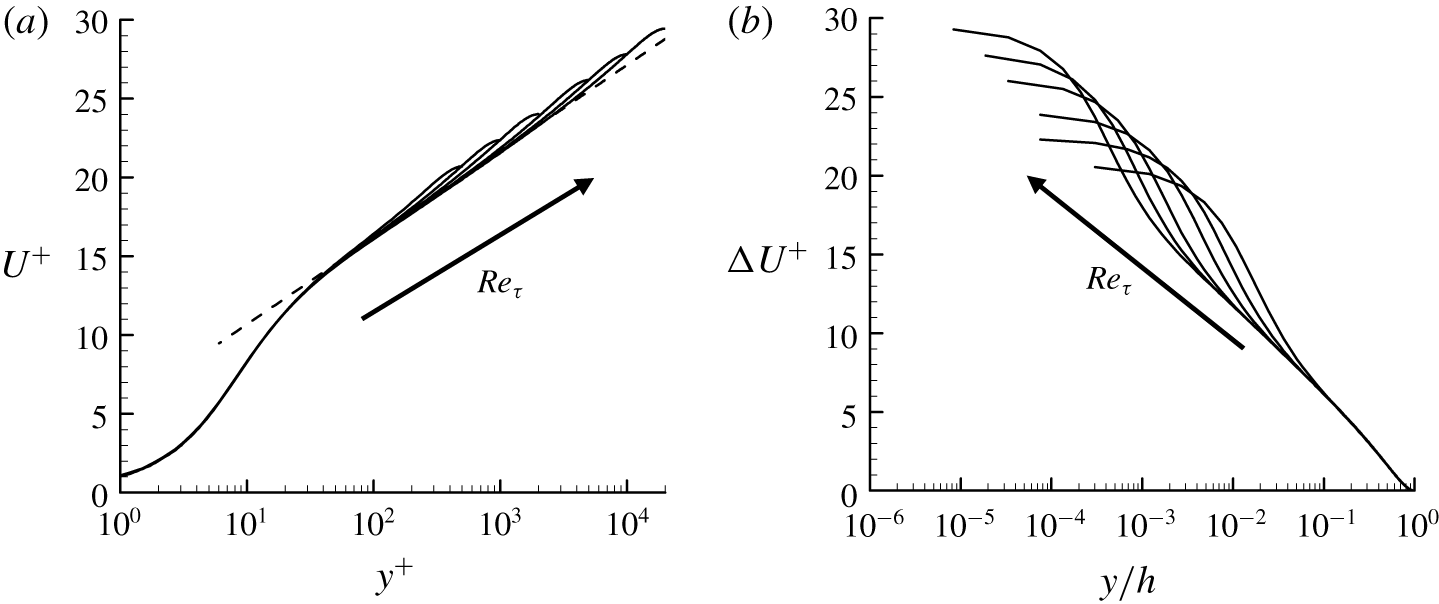
the mean velocity  $U(y)$ is obtained by solving (2.1a). Here, it should be noted that the closure (2.3) provides information only for the shear component of Reynolds stress. In § 2.3 we shall utilise this feature to recover the other components of Reynolds stress and their spanwise wavenumber spectra with the fluctuation equations (2.1b). In figure 1 we show the computed mean velocity in a range of the friction Reynolds number
 $Re_{\unicode[STIX]{x1D70F}}$ (
 $\equiv u_{\unicode[STIX]{x1D70F}}h/\unicode[STIX]{x1D708}$, where
 $u_{\unicode[STIX]{x1D70F}}=\sqrt{\unicode[STIX]{x1D70F}_{w}/\unicode[STIX]{x1D70C}}$). Although the computed mean velocity is obtained with a crude model for Reynolds shear stress (2.3), it firmly satisfies the law of the wall (figure 1a) and the velocity defect law (figure 1b) with a well-developed logarithmic layer.
Scaling of the model mean velocity: (a)  $U^{+}(y^{+})$; (b)
 $\unicode[STIX]{x0394}U^{+}(y/h)(\equiv U_{c}^{+}-U^{+}(y/h))$. Here,
 $Re_{\unicode[STIX]{x1D70F}}=500$, 1000, 2000, 5000, 10 000, 20 000. The dashed line indicates a log-law given by
 $U^{+}(y^{+})=1/0.426\log y^{+}+5.2$.

Once the mean velocity  $U(y)$ is obtained, the stochastic response of (2.1b) with the model of
 ${\mathcal{N}}$ in (2.2) can be computed. Let us consider the following stochastic forcing, white in both time and space:
 $$\begin{eqnarray}\displaystyle \langle \,\boldsymbol{f}^{\prime }(t,x,y,z){\boldsymbol{f}^{\prime }}^{\text{H}}(t^{\prime },x^{\prime },y^{\prime },z^{\prime })\rangle =\unicode[STIX]{x1D644}\unicode[STIX]{x1D6FF}(x-x^{\prime })\unicode[STIX]{x1D6FF}(y-y^{\prime })\unicode[STIX]{x1D6FF}(z-z^{\prime })\unicode[STIX]{x1D6FF}(t-t^{\prime }). & & \displaystyle\end{eqnarray}$$
Here  $\unicode[STIX]{x1D644}\in \mathbb{R}^{3\times 3}$ (
 $\mathbb{R}$ is the set of real numbers) denotes the identity matrix,
 $\langle \cdot \rangle$ an ensemble average and the superscript ‘H’ the complex conjugate transpose. Since (2.1b) with the model in (2.2) are linear and autonomous in the wall-parallel directions, it is convenient to take the following Fourier transform:
 $$\begin{eqnarray}\displaystyle \left.\begin{array}{@{}c@{}}\displaystyle \widehat{\boldsymbol{u}^{\prime }}(t,y;k_{x},k_{z})=\int _{-\infty }^{\infty }\int _{-\infty }^{\infty }\boldsymbol{u}^{\prime }(t,x,y,z)\text{e}^{-\text{i}(k_{x}x+k_{z}z)}\,\text{d}x\,\text{d}z,\\ \displaystyle \widehat{\boldsymbol{f}^{\prime }}(t,y;k_{x},k_{z})=\int _{-\infty }^{\infty }\int _{-\infty }^{\infty }\boldsymbol{f}^{\prime }(t,x,y,z)\text{e}^{-\text{i}(k_{x}x+k_{z}z)}\,\text{d}x\,\text{d}z.\end{array}\right\} & & \displaystyle\end{eqnarray}$$
Here the superscript ‘ $\widehat{\cdot }$’ indicates the Fourier-transformed state, and
 $k_{x}$ and
 $k_{z}$ are the streamwise and spanwise wavenumbers, respectively. In the Fourier space, (2.4) is then written as
 $$\begin{eqnarray}\displaystyle \langle \,\widehat{\boldsymbol{f}^{\prime }}(t,y;k_{x},k_{z})\widehat{\boldsymbol{f}^{\prime }}^{\text{H}}(t^{\prime },y^{\prime };k_{x},k_{z})\rangle =\unicode[STIX]{x1D644}\unicode[STIX]{x1D6FF}(y-y^{\prime })\unicode[STIX]{x1D6FF}(t-t^{\prime }). & & \displaystyle\end{eqnarray}$$
Once (2.1b) is solved in the Fourier space with the stochastic forcing (2.6), the power- and cross-spectral densities of velocity fluctuations are computed from the following spectral covariance matrix:
 $$\begin{eqnarray}\unicode[STIX]{x1D6F7}_{\boldsymbol{u}\boldsymbol{u}}(y,y^{\prime },k_{x},k_{z})\equiv \langle \widehat{\boldsymbol{u}^{\prime }}(t,y;k_{x},k_{z})\widehat{\boldsymbol{u}^{\prime }}^{\text{H}}(t,y^{\prime };k_{x},k_{z})\rangle .\end{eqnarray}$$
Here, we note that the time dependence in  $\unicode[STIX]{x1D6F7}_{\boldsymbol{u}\boldsymbol{u}}$ is now dropped because the ensemble average is equivalent to a time average in a statistically stationary setting, such as the present turbulent channel flow. The covariance matrix of velocity fluctuations is finally obtained by integrating the spectral covariance matrix over the Fourier space
 $$\begin{eqnarray}\langle \boldsymbol{u}^{\prime }{\boldsymbol{u}^{\prime }}^{\text{H}}\rangle (y,y^{\prime })=\frac{1}{4\unicode[STIX]{x03C0}^{2}}\int _{-\infty }^{\infty }\int _{-\infty }^{\infty }\unicode[STIX]{x1D6F7}_{\boldsymbol{u}\boldsymbol{u}}(y,y^{\prime };k_{x},k_{z})\,\text{d}k_{x}\,\text{d}k_{z},\end{eqnarray}$$
from which the Reynolds stress from the stochastic response is given with  $y=y^{\prime }$. We note that, in (2.8), the dependence of the covariance matrix on the streamwise and spanwise coordinates is dropped with the ensemble average.
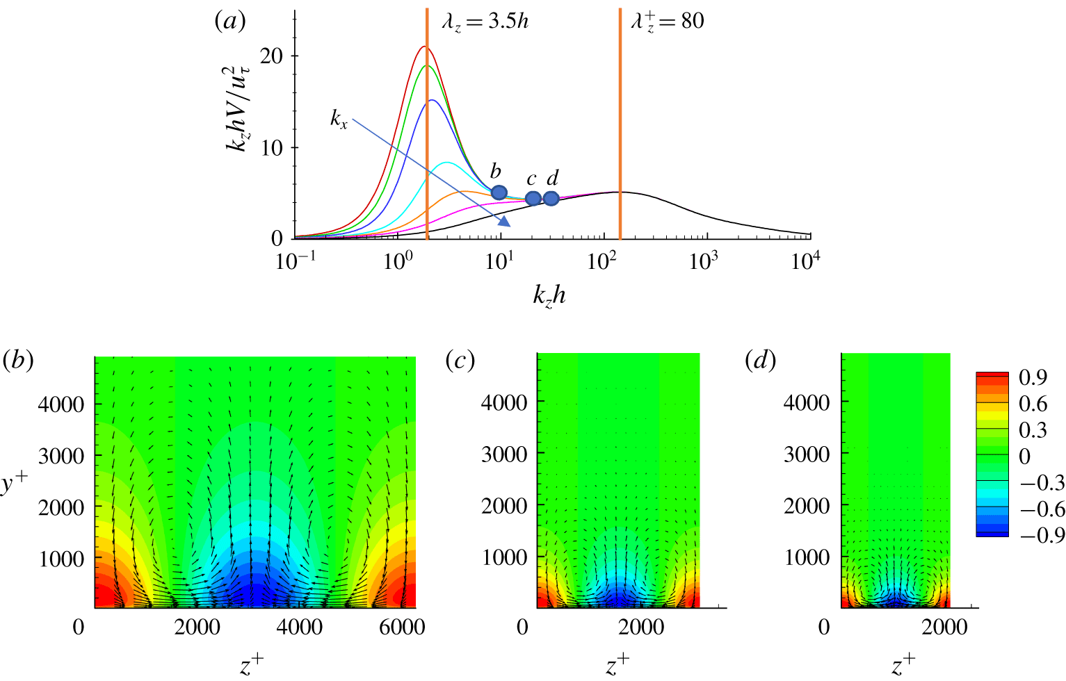
Response of the linear model to white noise in (2.4) at  $Re_{\unicode[STIX]{x1D70F}}=10^{4}$ (Hwang & Cossu Reference Hwang and Cossu2010b). (a) Premultiplied energy of all the POD modes,
 $k_{z}hV(k_{z})/u_{\unicode[STIX]{x1D70F}}^{2}$ (
 $k_{x}h=0.0$, 0.1, 0.2, 0.5, 1, 2, 5; the arrow indicates the increasing direction of
 $k_{x}$). (b–d) Cross-streamwise view of the leading POD mode at
 $k_{z}^{+}=0.001$, 0.002, 0.005 (
 $\unicode[STIX]{x1D706}_{z}^{+}=6283,3141,1256$) from left to right. In (b–d) the contours indicate streamwise velocity, and the vectors are cross-streamwise velocities. The velocity field of each POD mode is normalised by its maximum streamwise velocity.

The spectral covariance matrix of velocity fluctuations offers an important physical insight into the nature of the stochastic response. Let us compute POD modes in the Fourier space from the spectral covariance matrix
 $$\begin{eqnarray}\int _{0}^{2h}\unicode[STIX]{x1D6F7}_{\boldsymbol{u}\boldsymbol{u}}(y,y^{\prime },k_{x},k_{z})\widetilde{\boldsymbol{u}}_{j,POD}(y^{\prime };k_{x},k_{z})\,\text{d}y^{\prime }=\unicode[STIX]{x1D70E}_{j}(k_{x},k_{z})\widetilde{\boldsymbol{u}}_{j,POD}(y;k_{x},k_{z}),\end{eqnarray}$$
where  $\unicode[STIX]{x1D70E}_{j}(k_{x},k_{z})$ represents the energy of each POD mode sorted in descending order. The energy of all the POD modes, obtained by integrating over the wall-normal direction, is given by
 $$\begin{eqnarray}V(k_{x},k_{z})=\int _{0}^{2h}\text{trace}[\unicode[STIX]{x1D6F7}_{\boldsymbol{ u}\boldsymbol{u}}(y,y,k_{x},k_{z})]\,\text{d}y=\mathop{\sum }_{j=1}^{\infty }\unicode[STIX]{x1D70E}_{j}(k_{x},k_{z}).\end{eqnarray}$$
The energy  $V$ and the leading POD mode for each
 $k_{x}$ and
 $k_{z}$ are shown in figure 2 by replotting the data at
 $Re_{\unicode[STIX]{x1D70F}}=10\,000$ in Hwang & Cossu (Reference Hwang and Cossu2010b). In figure 2(a) the premultiplied energy
 $k_{z}V$ for several
 $k_{x}$ is plotted to show its density over the logarithmic
 $k_{z}$-axis. The premultiplied energy exhibits two peaks at
 $\unicode[STIX]{x1D706}_{z}(\equiv 2\unicode[STIX]{x03C0}/k_{z})=3.5h$ and
 $\unicode[STIX]{x1D706}_{z}^{+}=80$ (the superscript ‘+’ denotes normalisation made with
 $u_{\unicode[STIX]{x1D70F}}$ and
 $\unicode[STIX]{x1D6FF}_{\unicode[STIX]{x1D708}}(\equiv \unicode[STIX]{x1D708}/u_{\unicode[STIX]{x1D70F}})$), which scale well in outer and inner units, respectively. The outer peak is associated with the generation of very large-scale motions (Kim & Adrian Reference Kim and Adrian1999; del Álamo & Jiménez Reference del Álamo and Jiménez2003; Hutchins & Marusic Reference Hutchins and Marusic2007), whereas the inner peak well represents the near-wall streaks (Kline et al. Reference Kline, Reynolds, Schraub and Runstadler1967). Between the two, the premultiplied energy is approximately constant, and the leading POD modes obtained in this range of spanwise wavenumbers are self-similar with respect to
 $\unicode[STIX]{x1D706}_{z}$, as shown in figure 2(b–d). Each of the leading POD modes are in the form of strong streamwise velocity streaks with weak streamwise vortices due to the lift-up effect (see also Hwang & Cossu Reference Hwang and Cossu2010b). More quantitative scaling of these self-similar POD modes can be found in figure 4 of Hwang & Cossu (Reference Hwang and Cossu2010b). We also note that the leading POD modes here are almost identical to linear transient-growth modes and the resolvent modes (see Hwang & Cossu Reference Hwang and Cossu2010a,Reference Hwang and Cossub), and a comprehensive discussion on the scaling of the linear modes related to the logarithmic region can be found in Hwang (Reference Hwang2016).
2.3 Self-consistent determination of stochastic forcing
While the stochastic response discussed in § 2.2 provides a useful physical insight into the origin of coherent structures in turbulent channel flow, the linearised fluctuation equations (2.1b) with the stochastic forcing of (2.4) do not necessarily generate the Reynolds shear stress given by the mean equation (2.1a). However, it is important to realise that the mean and fluctuation equations (2.1a) and (2.1b) should share the same Reynolds shear stress, because they are derived from the same equations (i.e. the Navier–Stokes equations). This issue was evidently ignored in § 2.2 as well as in the previous studies (e.g. Hwang & Cossu Reference Hwang and Cossu2010b).
Perhaps the easiest way to resolve this issue would be to prescribe a carefully designed set of colour and amplitude of the stochastic forcing and then solve (2.1a) and (2.1b) simultaneously. However, in practice, there are too many possible choices for the colour and amplitude of the forcing to construct a statistically informative quasi-linear model. To overcome this difficulty, here we formulate an inverse problem under the assumption that the physically desirable mean velocity is available from an experimental measurement or from an empirical model shown in figure 1. With this setting, the Reynolds shear stress is obtained from the given mean velocity by solving (2.1a). Then, for the fluctuation dynamics to be consistent with the mean equation (2.1a), this Reynolds shear stress must be identical to the one from the fluctuation equations (2.1b). This naturally builds a necessary condition for the physically desirable stochastic forcing. Using this condition, we will now formulate an optimisation problem, which minimises the difference between the Reynolds shear stresses from (2.1a) and (2.1b), to determine the colour and amplitude of the stochastic forcing.
For simplicity, we start by considering a stochastic forcing with the following form of spectral covariance matrix:
 $$\begin{eqnarray}\langle \,\boldsymbol{f}^{\prime }(t,y;k_{x},k_{z}){\boldsymbol{f}^{\prime }}^{\text{H}}(t^{\prime },y^{\prime };k_{x},k_{z})\rangle =2\unicode[STIX]{x03C0}\unicode[STIX]{x1D6FF}(k_{x})W(k_{z})\unicode[STIX]{x1D644}\unicode[STIX]{x1D6FF}(y-y^{\prime })\unicode[STIX]{x1D6FF}(t-t^{\prime }).\end{eqnarray}$$
Here  $W(k_{z})\geqslant 0$ is an ‘unknown’ real-valued weight function, through which the colour in the spanwise direction and amplitude of the stochastic forcing will be determined. Here,
 $\unicode[STIX]{x1D6FF}(k_{x})$ is introduced to consider the streamwise Fourier modes for
 $k_{x}=0$ only. It should be mentioned that the assumption of considering only such Fourier modes is expected to yield highly anisotropic turbulence intensities strongly skewed to the streamwise component (see § 3.1). This is because the ignored streamwise Fourier modes with
 $k_{x}\neq 0$ plays the primary role in transporting turbulent kinetic energy from the streamwise to cross-streamwise components through the streamwise pressure-strain term (Cho et al. Reference Cho, Hwang and Choi2018). In real flow, this mechanism involves streak instability (or related transient growth), which has a strong correlation with activation of the streamwise pressure strain (Cho, Choi & Hwang Reference Cho, Choi and Hwang2016), and it is the key process for the generation of the cross-streamwise velocity components in the self-sustaining process (Hwang & Bengana Reference Hwang and Bengana2016; de Giovanetti, Sung & Hwang Reference de Giovanetti, Sung and Hwang2017). While it would be ideal to incorporate this mechanism into the present quasi-linear framework, the task does not appear to be simple to achieve, because the streak instability is a nonlinear process which requires coupling between the Fourier modes through (2.1c). If this nonlinear coupling is implemented, the superposition made available through the model of nonlinearity in (2.2) would not be possible, breaking the entire quasi-linear framework purposely developed to mimic the original attached eddy model. However, this does not imply that the streamwise Fourier modes for
 $k_{x}\neq 0$ cannot be used for the modelling purpose – they can still be used simply to mimic the statistical features of the streak instability without properly resolving its dynamics, although this modelling effort will be left for a future study to retain the simplicity of the present quasi-linear framework.
Since (2.1b) with  ${\mathcal{N}}$ in (2.2) is linear, the Reynolds stress tensor from the stochastic forcing of (2.11) is given by
 $$\begin{eqnarray}\langle \boldsymbol{u}^{\prime }{\boldsymbol{u}^{\prime }}^{\text{H}}\rangle (y)=\frac{1}{2\unicode[STIX]{x03C0}}\int _{-\infty }^{\infty }W(k_{z})\unicode[STIX]{x1D6F7}_{\boldsymbol{u}\boldsymbol{u}}(y,y;k_{x}=0,k_{z})\,\text{d}k_{z},\end{eqnarray}$$
and the resulting Reynolds shear stress is
 $$\begin{eqnarray}\displaystyle \langle u^{\prime }v^{\prime }\rangle (y) & = & \displaystyle \frac{1}{\unicode[STIX]{x03C0}}\int _{0}^{\infty }W(k_{z})\unicode[STIX]{x1D6F7}_{uv}(y,y;k_{x}=0,k_{z})\,\text{d}k_{z}\nonumber\\ \displaystyle & = & \displaystyle \frac{1}{\unicode[STIX]{x03C0}}\int _{-\infty }^{\infty }\text{e}^{\unicode[STIX]{x1D6FD}}W(\unicode[STIX]{x1D6FD})\unicode[STIX]{x1D6F7}_{uv}(y,y;k_{x}=0,\unicode[STIX]{x1D6FD})\,\text{d}\unicode[STIX]{x1D6FD},\end{eqnarray}$$
where  $\unicode[STIX]{x1D6FD}\equiv \log (k_{z})$ and
 $\unicode[STIX]{x1D6F7}_{uv}$ is the cross-spectral density component of
 $\unicode[STIX]{x1D6F7}_{\boldsymbol{u}\boldsymbol{u}}$ for the Reynolds shear stress. In turbulent channel flow, the smallest coherent structures are typically characterised by the spanwise length scale of
 $\unicode[STIX]{x1D706}_{z}^{+}\simeq 100$ (Kline et al. Reference Kline, Reynolds, Schraub and Runstadler1967), whereas the largest ones are featured with
 $\unicode[STIX]{x1D706}_{z}/h\simeq 1.5$ (del Álamo & Jiménez Reference del Álamo and Jiménez2003). To capture the wide range of the length scales of interest, the weight function
 $W(k_{z})$ is defined for
 $\unicode[STIX]{x1D706}_{z}\in [10\unicode[STIX]{x1D6FF}_{\unicode[STIX]{x1D708}},10h]$, while setting it to be zero at the boundaries. Without loss of generality, the weight function in the
 $\unicode[STIX]{x1D6FD}$-coordinate is written as
 $$\begin{eqnarray}W(k_{z}(\unicode[STIX]{x1D6FD}))=\mathop{\sum }_{n=1}^{N_{\unicode[STIX]{x1D6FD}}}a_{n}\sin (n\unicode[STIX]{x03C0}\unicode[STIX]{x1D709}(\unicode[STIX]{x1D6FD}))\quad \text{with}~\unicode[STIX]{x1D709}(\unicode[STIX]{x1D6FD})=\frac{\unicode[STIX]{x1D6FD}-\unicode[STIX]{x1D6FD}_{l}}{\unicode[STIX]{x1D6FD}_{u}-\unicode[STIX]{x1D6FD}_{l}},\end{eqnarray}$$
where  $N_{\unicode[STIX]{x1D6FD}}$ is the number of the sine polynomials,
 $a_{n}$ the polynomial coefficient,
 $\unicode[STIX]{x1D6FD}_{l}=\log (\unicode[STIX]{x03C0}/(5\unicode[STIX]{x1D6FF}_{\unicode[STIX]{x1D708}}))$ and
 $\unicode[STIX]{x1D6FD}_{u}=\log (\unicode[STIX]{x03C0}/(5h))$. The Reynolds shear stress generated by (2.1b) is then given by
 $$\begin{eqnarray}\langle u^{\prime }v^{\prime }\rangle (y)=\unicode[STIX]{x1D643}\boldsymbol{a},\end{eqnarray}$$
where  $\boldsymbol{a}=[a_{1}~~a_{2}~~a_{3}~~\cdots ~~a_{N_{\unicode[STIX]{x1D6FD}}}]^{\text{T}}$ and
 $$\begin{eqnarray}\displaystyle \unicode[STIX]{x1D643}=\frac{1}{\unicode[STIX]{x03C0}}\int _{-\infty }^{\infty }\text{e}^{\unicode[STIX]{x1D6FD}}\left[\begin{array}{@{}c@{}}\sin (\unicode[STIX]{x03C0}\unicode[STIX]{x1D709}(\unicode[STIX]{x1D6FD}))\unicode[STIX]{x1D731}_{uv}(y,y;k_{x}=0,\unicode[STIX]{x1D6FD})\\ \sin (2\unicode[STIX]{x03C0}\unicode[STIX]{x1D709}(\unicode[STIX]{x1D6FD}))\unicode[STIX]{x1D731}_{uv}(y,y;k_{x}=0,\unicode[STIX]{x1D6FD})\\ \cdots \\ \sin (N_{\unicode[STIX]{x1D6FD}}\unicode[STIX]{x03C0}\unicode[STIX]{x1D709}(\unicode[STIX]{x1D6FD}))\unicode[STIX]{x1D731}_{uv}(y,y;k_{x}=0,\unicode[STIX]{x1D6FD})\end{array}\right]^{\text{T}}\,\text{d}\unicode[STIX]{x1D6FD}. & & \displaystyle\end{eqnarray}$$
Now, let us formulate the optimisation problem to determine  $W(\unicode[STIX]{x1D6FD})$, the minimiser of the difference between
 $\overline{u^{\prime }v^{\prime }}(y)$ from (2.1a) and
 $\langle u^{\prime }v^{\prime }\rangle (y)$ from (2.15a). Here, it is important to note that a physically relevant
 $W(\unicode[STIX]{x1D6FD})$ must be sufficiently smooth. To ensure this property of
 $W(\unicode[STIX]{x1D6FD})$, we first solve the optimisation problem
 $$\begin{eqnarray}\min _{\boldsymbol{a}}\Vert \overline{u^{\prime }v^{\prime }}(y)-\unicode[STIX]{x1D643}\boldsymbol{a}\Vert _{Q}^{2}+\unicode[STIX]{x1D6FE}\boldsymbol{a}^{\text{T}}\boldsymbol{M}\boldsymbol{a}\end{eqnarray}$$
subject to
 $$\begin{eqnarray}W(k_{z}(\unicode[STIX]{x1D6FD}))\geqslant 0\quad \text{for all}~\unicode[STIX]{x1D6FD}\in [\unicode[STIX]{x1D6FD}_{l},\unicode[STIX]{x1D6FD}_{u}],\end{eqnarray}$$
where  $\unicode[STIX]{x1D6FE}\geqslant 0$ is the optimisation penalty balancing the first and second terms in (2.16a),
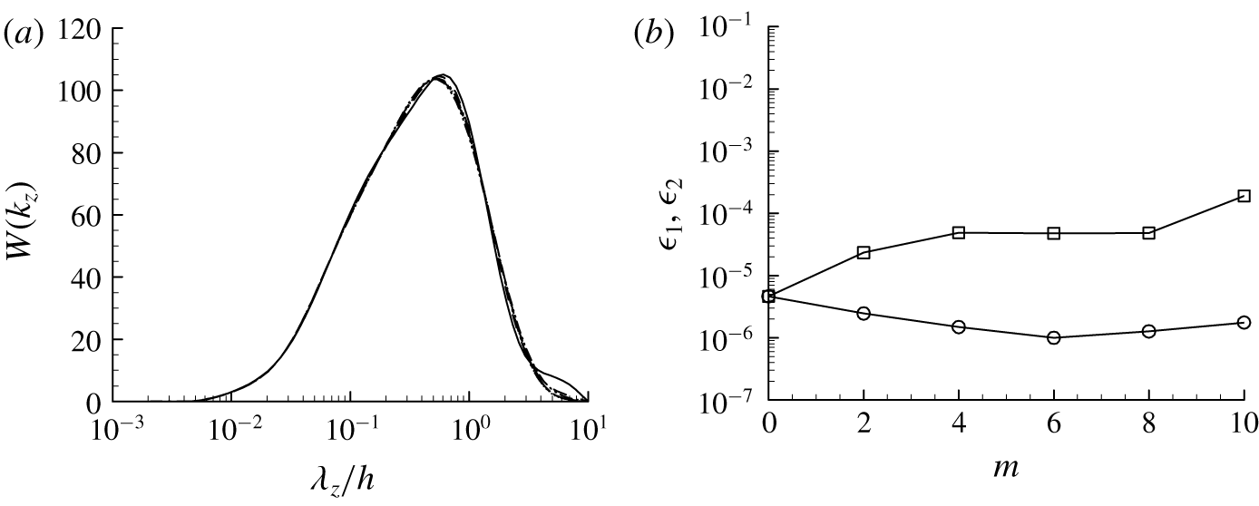
 $\boldsymbol{M}=\text{diag}[\text{e}^{\unicode[STIX]{x1D701}}~\text{e}^{2\unicode[STIX]{x1D701}}~\text{e}^{3\unicode[STIX]{x1D701}}\ldots \text{e}^{N_{\unicode[STIX]{x1D6FD}}\unicode[STIX]{x1D701}}]$ with
 $\unicode[STIX]{x1D701}=0.5$ chosen empirically, and
 $\Vert \cdot \Vert _{Q}^{2}=\int _{0}^{2h}(\cdot )^{2}Q(y)\,\text{d}y$ with
 $Q(y)=(y/h-1)^{6}$ introduced for a better optimisation result in the near-wall and logarithmic regions (for a detailed discussion on the choice of
 $\unicode[STIX]{x1D701}$ and
 $Q(y)$, see appendix). Here, it is evident that, if
 $\unicode[STIX]{x1D6FE}\rightarrow \infty$, the solution to (2.16) would ensure an exponential decay of
 $|a_{n}|$ with increasing
 $n$, resulting in a sufficiently smooth
 $W(k_{z}(\unicode[STIX]{x1D6FD}))$ with respect to
 $k_{z}$ (or
 $\unicode[STIX]{x1D6FD}$). However, in this case,
 $\Vert \overline{u^{\prime }v^{\prime }}(y)-\unicode[STIX]{x1D643}\boldsymbol{a}\Vert _{Q}^{2}$ in (2.16a) can easily be large, thereby not achieving the desired goal of the optimisation. By contrast, if
 $\unicode[STIX]{x1D6FE}\rightarrow 0$, the solution to (2.16) would yield a sufficiently small
 $\Vert \overline{u^{\prime }v^{\prime }}(y)-\unicode[STIX]{x1D643}\boldsymbol{a}\Vert _{Q}^{2}$, but it would not necessarily guarantee a sufficiently smooth
 $W(k_{z}(\unicode[STIX]{x1D6FD}))$ – such a situation can emerge especially if
 $N_{\unicode[STIX]{x1D6FD}}\rightarrow \infty$. In practice, it has been found that setting
 $\unicode[STIX]{x1D6FE}\rightarrow 0$ with finite
 $N_{\unicode[STIX]{x1D6FD}}$ also results in an unsatisfactorily large value of
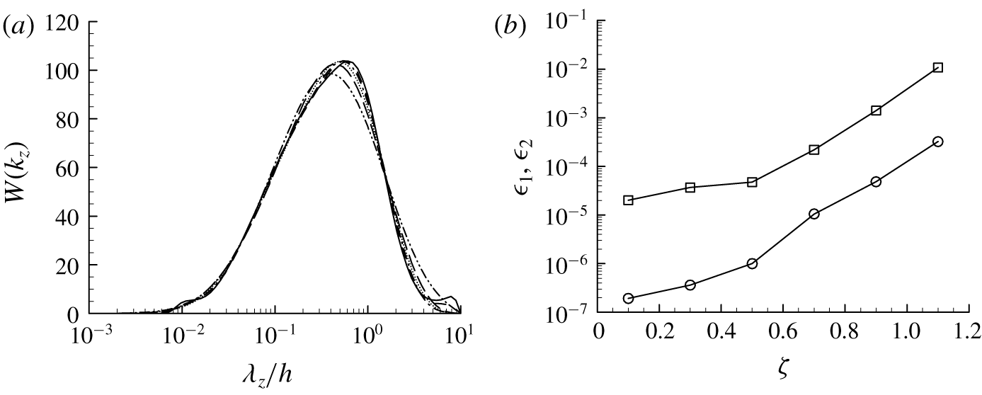
 $\Vert \overline{u^{\prime }v^{\prime }}(y)-\unicode[STIX]{x1D643}\boldsymbol{a}\Vert _{Q}^{2}$ (see also figure 3b). Based on this observation, here we solve another auxiliary optimisation problem which seeks the minimiser
 $\unicode[STIX]{x1D6FE}$ for the difference between
 $\overline{u^{\prime }v^{\prime }}(y)$ and
 $\langle u^{\prime }v^{\prime }\rangle (y)$, i.e.
 $$\begin{eqnarray}\unicode[STIX]{x1D6FE}_{opt}=\mathop{\text{arg min}}_{\unicode[STIX]{x1D6FE}}\Vert \overline{u^{\prime }v^{\prime }}(y)-\unicode[STIX]{x1D643}\boldsymbol{a}\Vert _{Q}^{2}.\end{eqnarray}$$
The weight function  $W(k_{z})$ in (2.11) is finally obtained from the solution to (2.16) for
 $\unicode[STIX]{x1D6FE}=\unicode[STIX]{x1D6FE}_{opt}$.
The overall solution procedure for the entire optimisation problem defined in (2.16) and (2.17) is given as follows.
(i) Choose
 $\unicode[STIX]{x1D6FE}$ and solve the optimisation problem (2.16).
(ii) For the chosen
$\unicode[STIX]{x1D6FE}$, evaluate the value of $\Vert \overline{u^{\prime }v^{\prime }}(y)-\unicode[STIX]{x1D643}\boldsymbol{a}\Vert _{Q}^{2}$ with the solution obtained from (i).(iii) Guess a new
$\unicode[STIX]{x1D6FE}$ and repeat (i) and (ii) until $\unicode[STIX]{x1D6FE}_{opt}$ is found by monitoring the value of $\Vert \overline{u^{\prime }v^{\prime }}(y)-\unicode[STIX]{x1D643}\boldsymbol{a}\Vert _{Q}^{2}$ at each iteration step (see also § 2.4 and figure 3b).


Here, steps (ii) and (iii) solve the optimisation problem (2.17). The details of the numerical method for each step will be presented in § 2.4.
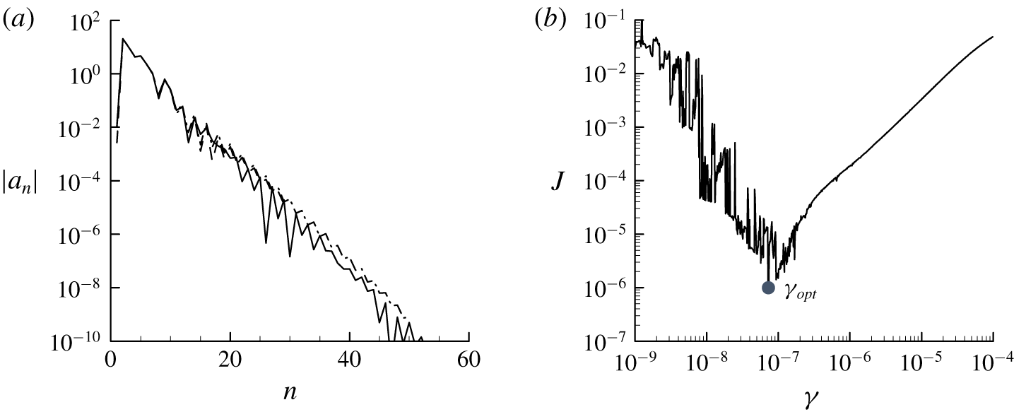
Optimisations (2.16) and (2.17) for a quasi-linear approximation at  $Re_{\unicode[STIX]{x1D70F}}=5000$ (
 $N_{POD}=2$): (a)
 $|a_{n}|$ for
 $W(\unicode[STIX]{x1D6FD})$ with respect
 $N_{\unicode[STIX]{x1D6FD}}$ (
 $\unicode[STIX]{x1D701}=0.5$); (b)
 $J$ versus
 $\unicode[STIX]{x1D6FE}$, where
 $J=\Vert \overline{u^{\prime }v^{\prime }}-\unicode[STIX]{x1D643}\boldsymbol{a}\Vert _{Q}^{2}$. In (a), – – – –,
 $N_{\unicode[STIX]{x1D6FD}}=30$; – ⋅ – ⋅ –,
 $N_{\unicode[STIX]{x1D6FD}}=50$; ——,
 $N_{\unicode[STIX]{x1D6FD}}=100$.

2.4 Numerical methods
The computation of the spectral covariance matrix is carried out by formulating the linearised Navier–Stokes equations (2.1b) with the model (2.2) in Fourier space in the form of the Orr–Sommerfeld–Squire system, i.e.
 $$\begin{eqnarray}\frac{\unicode[STIX]{x2202}\widehat{\boldsymbol{q}^{\prime }}}{\unicode[STIX]{x2202}t}=\unicode[STIX]{x1D63C}\widehat{\boldsymbol{q}^{\prime }}+\unicode[STIX]{x1D63D}\widehat{\boldsymbol{f}^{\prime }},\end{eqnarray}$$
where  $\widehat{\boldsymbol{q}^{\prime }}=[\widehat{v^{\prime }},\widehat{\unicode[STIX]{x1D714}_{y}^{\prime }}]^{\text{T}}$ and
 $$\begin{eqnarray}\displaystyle \unicode[STIX]{x1D63C}=\left[\begin{array}{@{}cc@{}}\unicode[STIX]{x1D6E5}^{-1}{\mathcal{L}}_{{\mathcal{O}}{\mathcal{S}}} & 0\\ -\text{i}\unicode[STIX]{x1D6FD}{\mathcal{D}}U & {\mathcal{L}}_{{\mathcal{S}}{\mathcal{Q}}}\end{array}\right],\quad \unicode[STIX]{x1D63D}=\left[\begin{array}{@{}ccc@{}}-\text{i}k_{x}\unicode[STIX]{x1D6E5}^{-1}{\mathcal{D}} & -k^{2}\unicode[STIX]{x1D6E5}^{-1} & -\text{i}k_{z}\unicode[STIX]{x1D6E5}^{-1}{\mathcal{D}}\\ \text{i}k_{z} & 0 & -\text{i}k_{x}\end{array}\right] & & \displaystyle\end{eqnarray}$$
with
 $$\begin{eqnarray}\displaystyle & {\mathcal{L}}_{{\mathcal{O}}{\mathcal{S}}}=-\text{i}k_{x}(U\unicode[STIX]{x1D6E5}-{\mathcal{D}}^{2}U)+\unicode[STIX]{x1D708}_{T}\unicode[STIX]{x1D6E5}^{2}+2({\mathcal{D}}\unicode[STIX]{x1D708}_{T})\unicode[STIX]{x0394}{\mathcal{D}}+({\mathcal{D}}^{2}\unicode[STIX]{x1D708}_{T})({\mathcal{D}}^{2}+k^{2}), & \displaystyle\end{eqnarray}$$
 $$\begin{eqnarray}\displaystyle & {\mathcal{L}}_{{\mathcal{S}}{\mathcal{Q}}}=-\text{i}k_{x}U+\unicode[STIX]{x1D708}_{T}\unicode[STIX]{x1D6E5}+({\mathcal{D}}\unicode[STIX]{x1D708}_{T}){\mathcal{D}}. & \displaystyle\end{eqnarray}$$
Here,  $\hat{\unicode[STIX]{x1D714}}_{y}$ is the wall-normal vorticity of
 $\hat{\boldsymbol{u}}(y,t)$,
 $\unicode[STIX]{x1D6E5}={\mathcal{D}}^{2}-k^{2}$,
 $k^{2}=k_{x}^{2}+k_{z}^{2}$,
 ${\mathcal{D}}$ denotes
 $\unicode[STIX]{x2202}/\unicode[STIX]{x2202}y$. Using
 $\widehat{\boldsymbol{q}^{\prime }}$, the velocity fluctuation is obtained from
 $$\begin{eqnarray}\displaystyle \widehat{\boldsymbol{u}^{\prime }}=\unicode[STIX]{x1D63E}\widehat{\boldsymbol{q}^{\prime }},\quad \unicode[STIX]{x1D63E}=\frac{1}{k^{2}}\left[\begin{array}{@{}cc@{}}\text{i}k_{x}{\mathcal{D}} & -\text{i}k_{z}\\ k^{2} & 0\\ \text{i}k_{z}{\mathcal{D}} & \text{i}k_{x}\end{array}\right]. & & \displaystyle\end{eqnarray}$$
Following the adjoint-based formulation in Balakrishnan (Reference Balakrishnan1981), the spectral covariance matrix of the stochastic response is given as the solution to the following algebraic Lyapunov equation (for further details on this approach, see also the recent review by Zare, Georgiou & Jovanović (Reference Zare, Georgiou and Jovanović2020)):
 $$\begin{eqnarray}\unicode[STIX]{x1D63C}\boldsymbol{X}_{\infty }+\boldsymbol{X}_{\infty }\unicode[STIX]{x1D63C}^{\dagger }+\unicode[STIX]{x1D63D}\unicode[STIX]{x1D63D}^{\dagger }=0\end{eqnarray}$$
with
 $$\begin{eqnarray}\boldsymbol{X}_{\infty }\widehat{\boldsymbol{s}}=\int _{0}^{2h}\langle \widehat{\boldsymbol{q}^{\prime }}(t,y;k_{x},k_{z})\widehat{\boldsymbol{q}^{\prime }}^{\text{H}}(t,y^{\prime };k_{x},k_{z})\rangle \widehat{\boldsymbol{s}}(y^{\prime })\,\text{d}y^{\prime },\end{eqnarray}$$
where  $\widehat{\boldsymbol{s}}$ is an arbitrary two-dimensional complex vector function, ‘†’ indicates the adjoint with respect to the standard inner product,
 $\int _{0}^{2h}\widehat{\boldsymbol{m}}^{\text{H}}(y)\widehat{\boldsymbol{n}}(y)\,\text{d}y$ with
 $\widehat{\boldsymbol{m}}$ and
 $\widehat{\boldsymbol{n}}$ being arbitrary three-dimensional complex vector functions. The solution to (2.19) yields the following form for the spectral covariance matrix:
 $$\begin{eqnarray}\int _{0}^{2h}\unicode[STIX]{x1D6F7}_{\boldsymbol{u}\boldsymbol{u}}(y,y^{\prime },k_{x},k_{z})\widehat{\boldsymbol{m}}(y^{\prime })\,\text{d}y^{\prime }=\unicode[STIX]{x1D63E}\boldsymbol{X}_{\infty }\unicode[STIX]{x1D63E}^{\dagger }\widehat{\boldsymbol{m}}.\end{eqnarray}$$
It is also useful to write the spectral covariance matrix in terms of the POD modes
 $$\begin{eqnarray}\unicode[STIX]{x1D6F7}_{\boldsymbol{u}\boldsymbol{u}}(y,y^{\prime },k_{x},k_{z})=\mathop{\sum }_{j=1}^{N_{POD}}\unicode[STIX]{x1D70E}_{j}(k_{x},k_{z})\widetilde{\boldsymbol{u}}_{j,POD}(y;k_{x},k_{z})\widetilde{\boldsymbol{u}}_{j,POD}^{\text{H}}(y^{\prime };k_{x},k_{z}),\end{eqnarray}$$
where  $N_{POD}$ is the number of the POD modes used. In § 3.1 we shall see that (2.20b) offers an extra design choice for the spectral covariance matrix. In particular, this expression conveniently enables the suppression of an unphysical artefact in the spectral covariance matrix of the present quasi-linear model caused by the crude representation of
 ${\mathcal{N}}$ in (2.2).
The spectral covariance matrix is computed using the numerical solver developed in Hwang & Cossu (Reference Hwang and Cossu2010a,Reference Hwang and Cossub). The wall-normal direction is discretised with a Chebyshev collocation method (Weideman & Reddy Reference Weideman and Reddy2000). The resulting discretised Lyapunov equation in (2.19) is solved using the function lyap in MATLAB. The sampling of the spanwise wavenumber is made to be spaced logarithmically in the  $k_{z}$-coordinate (i.e. uniformly in the
 $\unicode[STIX]{x1D6FD}$-coordinate), and the integrals in (2.15b) are evaluated in the
 $\unicode[STIX]{x1D6FD}$-coordinate using the trapezoidal rule. The sampling resolution is maintained to be lower than
 $\unicode[STIX]{x0394}\unicode[STIX]{x1D6FD}=0.05$, so that the errors from the numerical integrations do not exceed more than
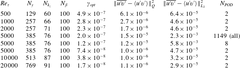
 $O(\unicode[STIX]{x0394}\unicode[STIX]{x1D6FD}^{2})$. The numbers of the wall-normal grid points and the sampling points in the spanwise wavenumber space are summarised in table 1.
Computational parameters and the optimisation errors in the present study:  $N_{y}$ is the number of wall-normal grid points,
 $N_{k_{z}}$ is the number of spanwise wavenumbers spaced logarithmically along the
 $k_{z}$ axis and
 $\Vert \cdot \Vert _{L_{2}}$ is the standard
 $L_{2}$ norm.

It is not difficult to recognise that the optimisation (2.16) is a standard quadratic programming problem (Luenberger & Ye Reference Luenberger and Ye2016) and is solved using the function quadprog in MATLAB. The effect of the number of sine polynomials  $N_{\unicode[STIX]{x1D6FD}}$ is also tested, as reported in figure 3(a). As expected from the form of
 $\unicode[STIX]{x1D63D}$ in (2.16a), the absolute value of the polynomial coefficients
 $|a_{n}|$ decays exponentially with
 $n$. Good convergence of
 $W(k_{z})$ is typically obtained for
 $N_{\unicode[STIX]{x1D6FD}}\gtrsim 30$, and
 $N_{\unicode[STIX]{x1D6FD}}=100$ is used in the present study. The effect of
 $\unicode[STIX]{x1D6FE}$ in the penalty term is also examined, as shown in figure 3(b). As discussed in § 2.3, there exists an optimal value of
 $\unicode[STIX]{x1D6FE}$ (i.e.
 $\unicode[STIX]{x1D6FE}_{opt}$) which minimises
 $\Vert \overline{u^{\prime }v^{\prime }}-\unicode[STIX]{x1D643}\boldsymbol{a}\Vert _{Q}^{2}$. The value of
 $\unicode[STIX]{x1D6FE}_{opt}$ is found using a simple line search over the logarithmic
 $\unicode[STIX]{x1D6FE}$-axis.
3 Results and discussion
3.1 Quasi-linear approximation at $Re_{\unicode[STIX]{x1D70F}}=5000$

The proposed QLA model is solved at  $Re_{\unicode[STIX]{x1D70F}}=5000$, and its performance is first assessed with the DNS data of Lee & Moser (Reference Lee and Moser2015) at
 $Re_{\unicode[STIX]{x1D70F}}=5186$. The computed weight function
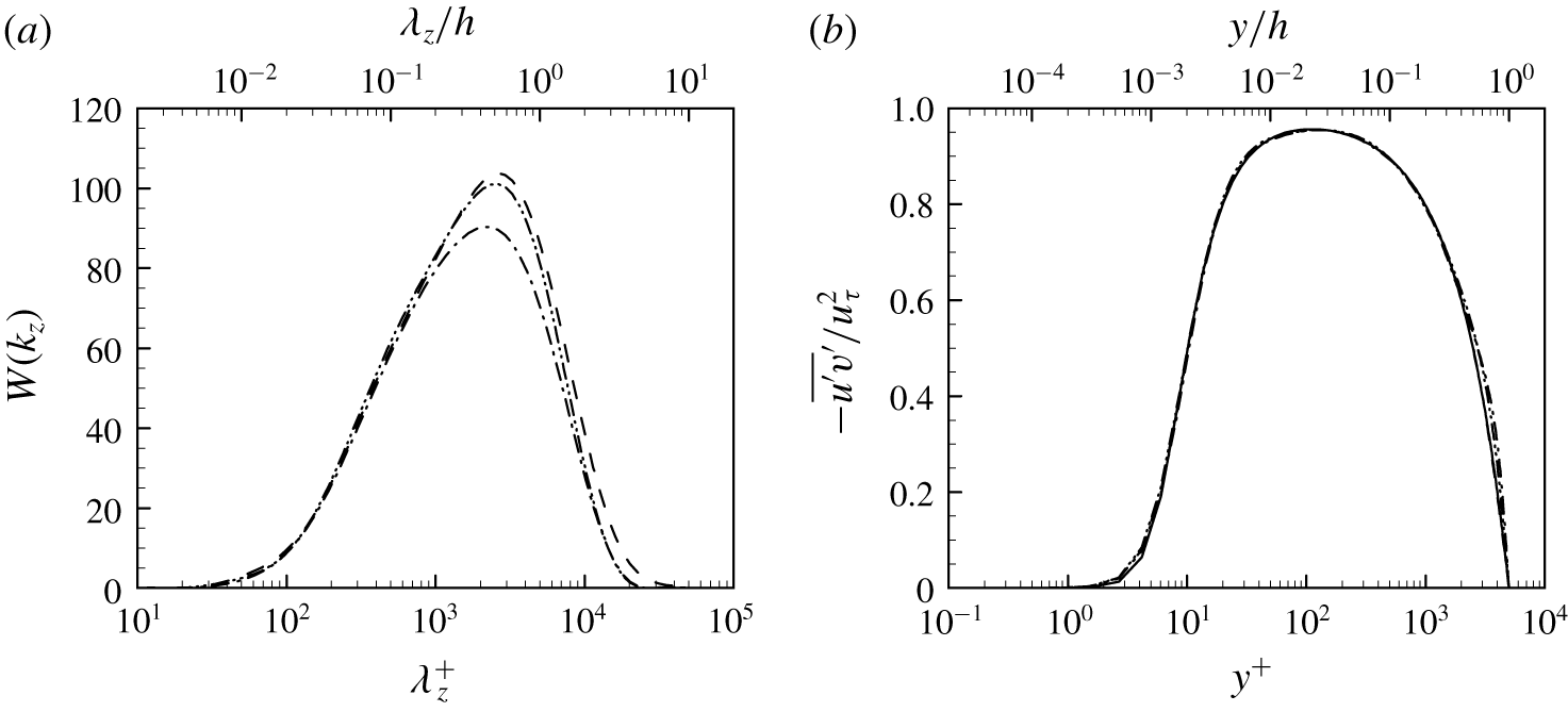
 $W(k_{z})$ and the resulting Reynolds shear stress are shown in figure 4. The weight function
 $W(k_{z})$ is found to be sufficiently smooth and well manifested within the interval between
 $\unicode[STIX]{x1D706}_{z}^{+}=10$ and
 $\unicode[STIX]{x1D706}_{z}/h=10$ (figure 4a), indicating that the domain of
 $W(k_{z})$ is sufficiently wide in the
 $k_{z}$-axis. The effect of
 $N_{POD}$ used for the construction of the spectral covariance matrix (see (2.20b)) is also examined for
 $N_{POD}=2$, 8, 1149 (note that
 $N_{POD}$ must be an even number for sufficiently small
 $N_{POD}$ because the even symmetry about the midplane yields two symmetric POD modes located in the lower and upper parts of the channel, respectively; see Hwang & Cossu Reference Hwang and Cossu2010b). It is seen that
 $N_{POD}$ does not affect the smoothness of
 $W(k_{z})$ (figure 4a) nor its overall shape. For all
 $N_{POD}$ considered, the Reynolds shear stress obtained with the computed
 $W(k_{z})$ also exhibits good agreement with the one from the mean equation (2.1a). In particular, the best agreement is obtained when
 $N_{POD}=2$ (table 1).
Quasi-linear approximations at  $Re_{\unicode[STIX]{x1D70F}}=5000$: (a)
 $W(k_{z})$ computed with (2.16) and (2.17); (b) comparison of the Reynolds shear stress from the mean equation (2.1a) and the fluctuation equations (2.1b). Here, ——,
 $-\overline{u^{\prime }v^{\prime }}$ from (2.1a); – – – –,
 $-\langle u^{\prime }v^{\prime }\rangle$ from (2.13) with
 $N_{POD}=2$; – ⋅ – ⋅ –, with
 $N_{POD}=8$; – ⋅⋅ – ⋅⋅ –, with
 $N_{POD}=1149$.

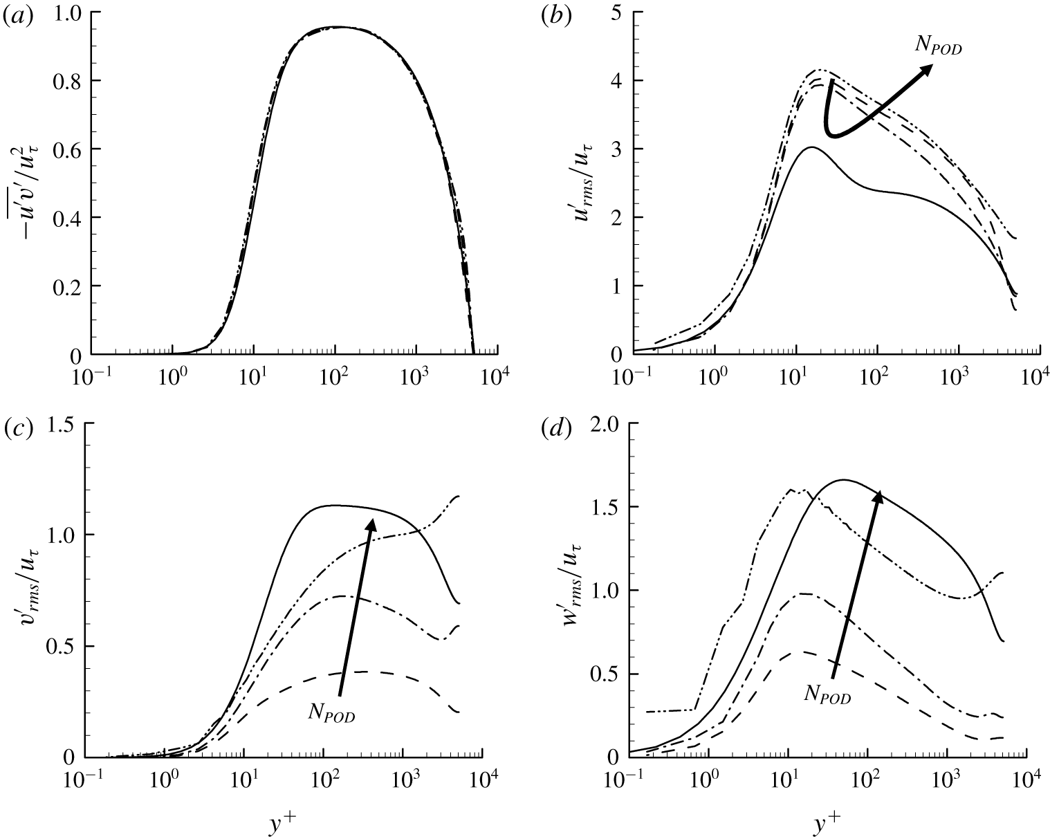
In figure 5 we compare the Reynolds stresses of the present QLA with those of DNS by Lee & Moser (Reference Lee and Moser2015). For all the cases of  $N_{POD}$ considered, the Reynolds shear stress from the fluctuation equations (2.1b) shows good agreement with that of DNS (figure 5a), indicating that the model mean velocity shown in figure 1 is a reasonable approximation to the real one at least around
 $Re_{\unicode[STIX]{x1D70F}}=5000$ (note that the model mean velocity is originally tuned to have the best match with DNS data at
 $Re_{\unicode[STIX]{x1D70F}}=2003$; see del Álamo & Jiménez Reference del Álamo and Jiménez2006). As expected, the velocity fluctuations of the present QLA show non-negligible differences from those of DNS. In particular, they exhibit the typical features observed in different types of QLAs, such as S3T (Farrell & Ioannou Reference Farrell and Ioannou2012) and RNL (Thomas et al. Reference Thomas, Farrell, Ioannou and Gayme2015; Farrell et al. Reference Farrell, Ioannou, Jiménez, Constantinou, Lozano-Durán and Nikolaidis2016): the streamwise velocity fluctuation of the present QLA tends to be larger than that of DNS (figure 5b), whereas its wall-normal and spanwise ones are smaller than those of DNS (figure 5c,d). This is, however, not surprising at least in the present QLA because this appears to be a consequence of ignoring all the streamwise varying Fourier modes (see (2.11)). Indeed, in real flow, the ignored streamwise Fourier modes for
 $k_{x}\neq 0$ are responsible for resolving the streak instability in the self-sustaining process (Hwang & Bengana Reference Hwang and Bengana2016; Cassinelli, de Giovanetti & Hwang Reference Cassinelli, de Giovanetti and Hwang2017; de Giovanetti et al. Reference de Giovanetti, Sung and Hwang2017), and they play a key role in transferring the turbulent kinetic energy produced at the streamwise component to the other components (Cho et al. Reference Cho, Hwang and Choi2018). As
 $N_{POD}$ is increased, the velocity fluctuations tend to be more isotropic and their anisotropic extent becomes closer to that of DNS. However, this does not necessarily imply that the increase of
 $N_{POD}$ improves the proposed QLA – this is simply because the higher-order POD modes are more isotropic than the lower-order ones. In fact, both the wall-normal and spanwise velocity fluctuations also develop a non-physical peak in the outer region for
 $N_{POD}\geqslant 8$ (
 $y^{+}\geqslant 2000$ in figure 5c,d).
Second-order turbulence statistics of DNS at  $Re_{\unicode[STIX]{x1D70F}}=5186$ (Lee & Moser Reference Lee and Moser2015) and QLA at
 $Re_{\unicode[STIX]{x1D70F}}=5000$: (a)
 $-\overline{u^{\prime }v^{\prime }}/u_{\unicode[STIX]{x1D70F}}^{2}$; (b)
 $u_{rms}^{\prime }/u_{\unicode[STIX]{x1D70F}}$; (c)
 $v_{rms}^{\prime }/u_{\unicode[STIX]{x1D70F}}$; (d)
 $w_{rms}^{\prime }/u_{\unicode[STIX]{x1D70F}}$. Here, ——, DNS; – – – –,
 $N_{POD}=2$; – ⋅ – ⋅ –,
 $N_{POD}=8$; – ⋅⋅ – ⋅⋅ –,
 $N_{POD}=1149$ (all).

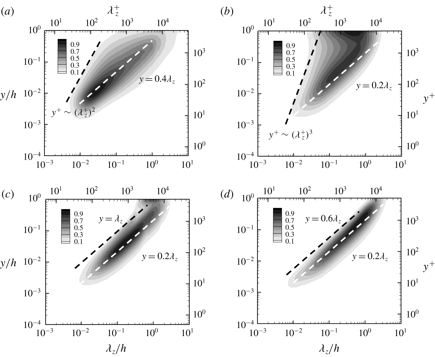
Spanwise wavenumber spectra of wall-normal velocity from (a) DNS at  $Re_{\unicode[STIX]{x1D70F}}=5186$ (Lee & Moser Reference Lee and Moser2015) and from (b–d) QLA at
 $Re_{\unicode[STIX]{x1D70F}}=5000$. Here, (b)
 $N_{POD}=1149$ (all); (c)
 $N_{POD}=8$; (d)
 $N_{POD}=2$. The contours are normalised by their maximum value, and their levels are spaced with 10 % of the maximum.

To further understand the effect of  $N_{POD}$ on the velocity fluctuations, spanwise wavenumber spectra of the wall-normal velocity of DNS are further compared with those of QLA. The energy-containing part of the spectra of DNS shows good alignment along a ridge scaling with
 $y$ linearly (
 $y=0.4\unicode[STIX]{x1D706}_{z}$ in figure 6a), consistent with the attached eddy hypothesis. The spectra of the present QLA show qualitatively the same behaviour for all
 $N_{POD}$ considered – they are also aligned well with a linear ridge
 $y=0.2\unicode[STIX]{x1D706}_{z}$ (figure 6b–d). However, the spectra of DNS show significant differences from those of QLA in the region where the energy cascade for turbulent dissipation is supposed to play an important role in the formation of the spectra: i.e.
 $y>0.4\unicode[STIX]{x1D706}_{z}$ in figure 6(a) and
 $y>0.2\unicode[STIX]{x1D706}_{z}$ in figure 6(b–d) (see also Cho et al. Reference Cho, Hwang and Choi2018). In this region, the low-level contour lines of the DNS spectra (e.g. 10 % contour level in figure 6a) appear to be aligned well with
 $y\sim \unicode[STIX]{x1D706}_{z}^{2}$, which would depict the Taylor microscale in the logarithmic region. By contrary, the spectra of the QLA with
 $N_{POD}=1149$ (figure 6b) do not show such a behaviour. Instead, they contain the primary peak at the channel centre, and their low-level contour lines oddly scale with
 $y\sim \unicode[STIX]{x1D706}_{z}^{3}$. It is evident that these are the unphysical artefact caused by the crude model for
 ${\mathcal{N}}$ in (2.2). For example, in DNS or in real flow, the turbulence production is zero at the channel centre, thus it is very unlikely to have any strong velocity fluctuations at this location. By contrary, the QLA still has a driving mechanism of velocity fluctuations at this location because the considered stochastic forcing has a non-zero amplitude (see (2.11)). This explains why the QLA exhibits a peak in the wall-normal and spanwise velocity fluctuations when relatively large
 $N_{POD}$ is used for the spectral covariance matrix (figure 5b,c). This artefact can simply be removed by considering only a few leading POD modes for the construction of the spectral covariance matrix, as shown in figure 6(d) where
 $N_{POD}=2$ is used. By doing so, all the contour lines of the spectra are very well aligned with
 $y=0.2\unicode[STIX]{x1D706}_{z}$, indicating that only the energy-containing part is now accounted for modelling of the velocity fluctuations like the original attached eddy model of Townsend (Reference Townsend1976). This observation suggests that only a few leading POD modes are self-similar and the rest of the modes are not. Furthermore, taking
 $N_{POD}=2$ has been found to significantly lower the error in the solution to the proposed optimisation problems (2.16) and (2.17) (table 1), implying that these non-self-similar higher-order POD modes, presumably an unphysical artefact of the crude model of
 ${\mathcal{N}}$, only deteriorates the performance of the optimisation problems. Therefore, from now on, we shall only consider
 $N_{POD}=2$ for the QLA in the present study.
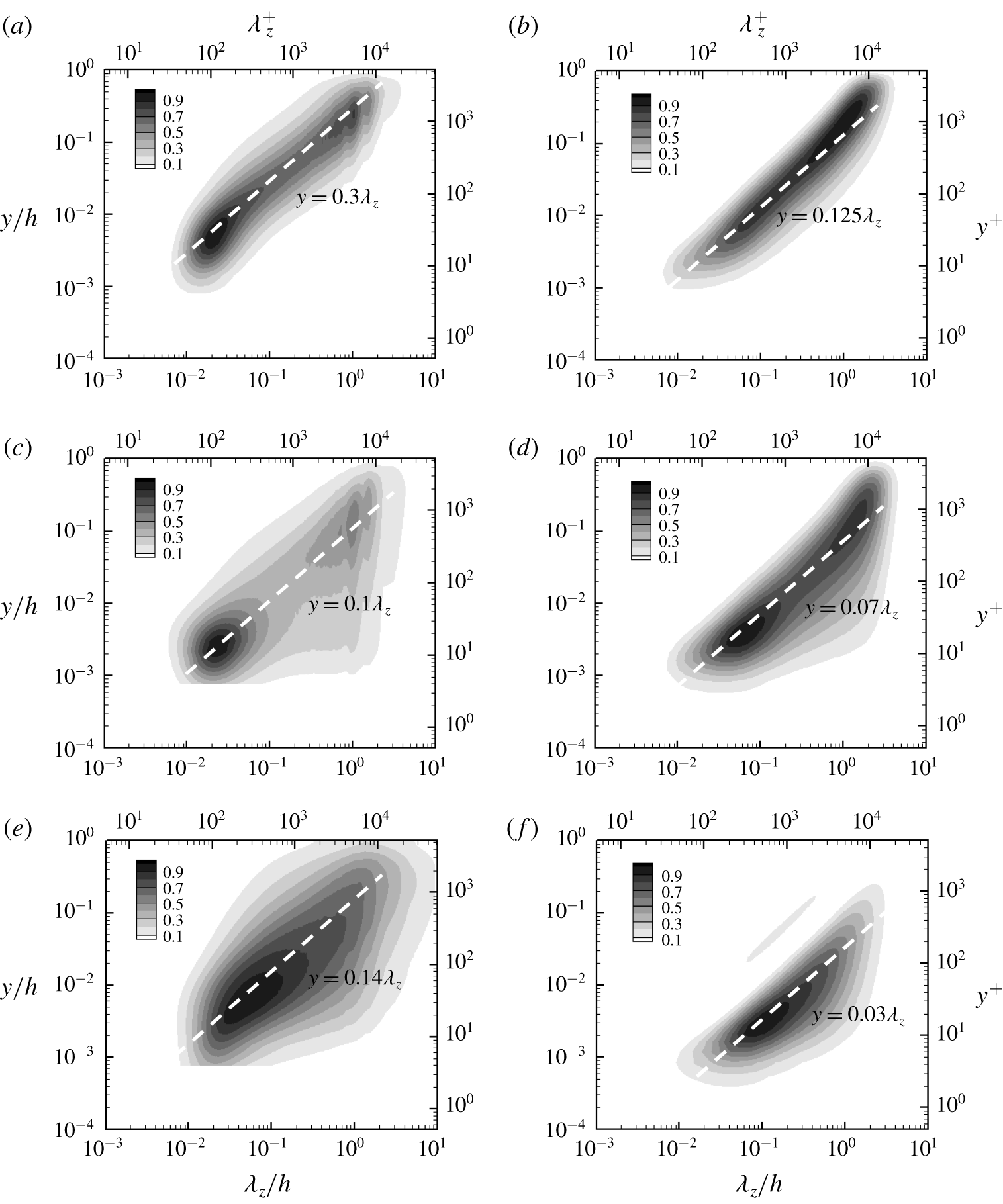
Spanwise wavenumber spectra from (a,c,e) DNS at  $Re_{\unicode[STIX]{x1D70F}}=5186$ (Lee & Moser Reference Lee and Moser2015) and (b,d,f) QLA (
 $N_{POD}=2$) at
 $Re_{\unicode[STIX]{x1D70F}}=5000$: (a,b) Reynolds shear stress; (c,d) streamwise velocity; (e,f) spanwise velocity. The contours are normalised by their maximum value, and their levels are spaced with 10 % of the maximum.

In figure 7 we further compare the spanwise wavenumber spectra of the other Reynolds-stress components from DNS with those from the QLA. In general, the energy-containing part of each spectra from both DNS and QLA appears to be well aligned with a linearly scaling ridge with  $y$. Furthermore, in both cases, the spectra of the streamwise and spanwise turbulent kinetic energies tend to contribute to the near-wall region for large
 $\unicode[STIX]{x1D706}_{z}$, unlike the wall-normal velocity spectra in figure 6 and the Reynolds shear-stress spectra in figure 7(a,b); for example, 10 % contour lines of these spectra reach
 $y^{+}\lesssim 10$ at
 $\unicode[STIX]{x1D706}_{z}\simeq 1h$ (figure 7c–f). This wall-reaching part of the streamwise and spanwise turbulent kinetic energies describes the so-called ‘inactive’ motion in the sense of Townsend (Reference Townsend1976), and its wall-normal distribution has been shown to scale in inner units, resulting in a ‘mesolayer’-like behaviour in the spectra (for a detailed discussion on the scaling and the origin of this part, see Hwang (Reference Hwang2016), Cho et al. (Reference Cho, Hwang and Choi2018)).
Despite the qualitatively good comparison between the DNS and QLA spectra, it should be pointed out that the detailed features of the spectra of the QLA are still non-negligibly different from those of DNS. In particular, the linear ridges of the QLA, along which the spectra are aligned in the  $\unicode[STIX]{x1D706}_{z}$–
 $y$ plane, tend to appear in the region closer to the wall than those of DNS: all the scaling constants for the linear ridge of the QLA spectra are smaller than those of the DNS (figures 6 and 7). While this difference partially originates from the crude nature of the model for
 ${\mathcal{N}}$ in (2.2), the other important reason is the lack of the description of the streak instability in the present QLA. Indeed, the streak instability mechanism has been shown to generate a strong wall-normal and spanwise velocity fluctuation (Cassinelli et al. Reference Cassinelli, de Giovanetti and Hwang2017; de Giovanetti et al. Reference de Giovanetti, Sung and Hwang2017), and their contribution to the spanwise wavenumber spectra appears roughly along
 $y=0.5\unicode[STIX]{x1D706}_{z}$ located much further from
 $y=0.2\unicode[STIX]{x1D706}_{z}$ in figure 6 and
 $y=0.03\unicode[STIX]{x1D706}_{z}$ in figure 7(f) (for a detailed discussion, see Hwang Reference Hwang2015). However, the incorporation of the streak instability mechanism into the present QLA is not straightforward because this mechanism is primarily mediated by
 ${\mathcal{N}}$ in (2.1c) (de Giovanetti et al. Reference de Giovanetti, Sung and Hwang2017) – if
 ${\mathcal{N}}$ becomes nonlinear, (2.12) is no longer true, breaking the entire quasi-linear framework.
3.2 Scaling with Reynolds number
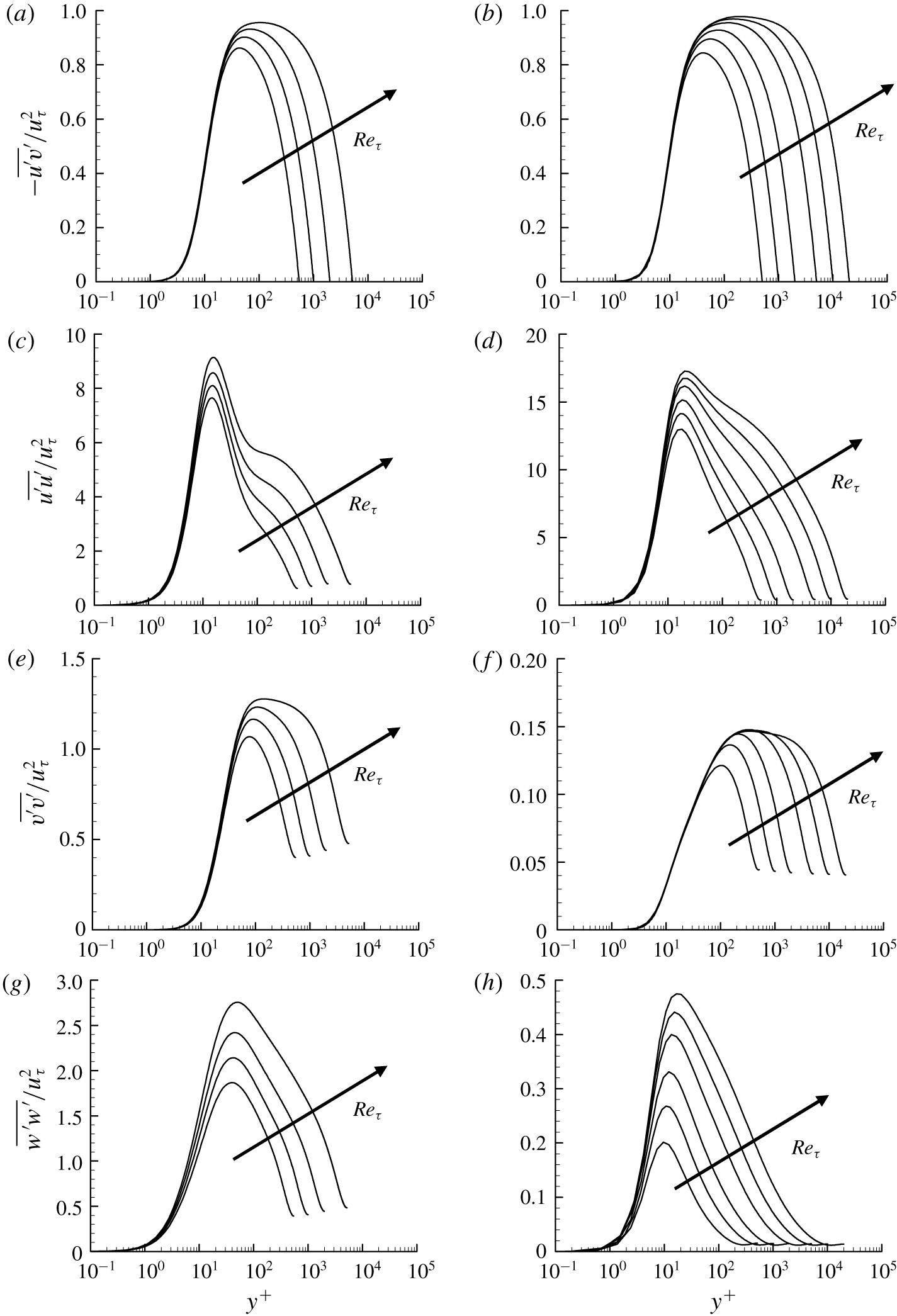
Reynolds-stress profile from (a,c,e,g) DNS (Lee & Moser Reference Lee and Moser2015) and (b,d,f,h) QLA ( $N_{POD}=2$) in the inner-scaled wall-normal coordinate: (a,b)
 $-\overline{u^{\prime }v^{\prime }}/u_{\unicode[STIX]{x1D70F}}^{2}$; (c,d)
 $\overline{u^{\prime }u^{\prime }}/u_{\unicode[STIX]{x1D70F}}^{2}$; (e,f)
 $\overline{v^{\prime }v^{\prime }}/u_{\unicode[STIX]{x1D70F}}^{2}$; (g,h)
 $\overline{w^{\prime }w^{\prime }}/u_{\unicode[STIX]{x1D70F}}^{2}$. Here,
 $Re_{\unicode[STIX]{x1D70F}}=543$, 1001, 1995, 5186 for DNS and
 $Re_{\unicode[STIX]{x1D70F}}=500$, 1000, 2000, 5000, 10 000, 20 000 for QLA.

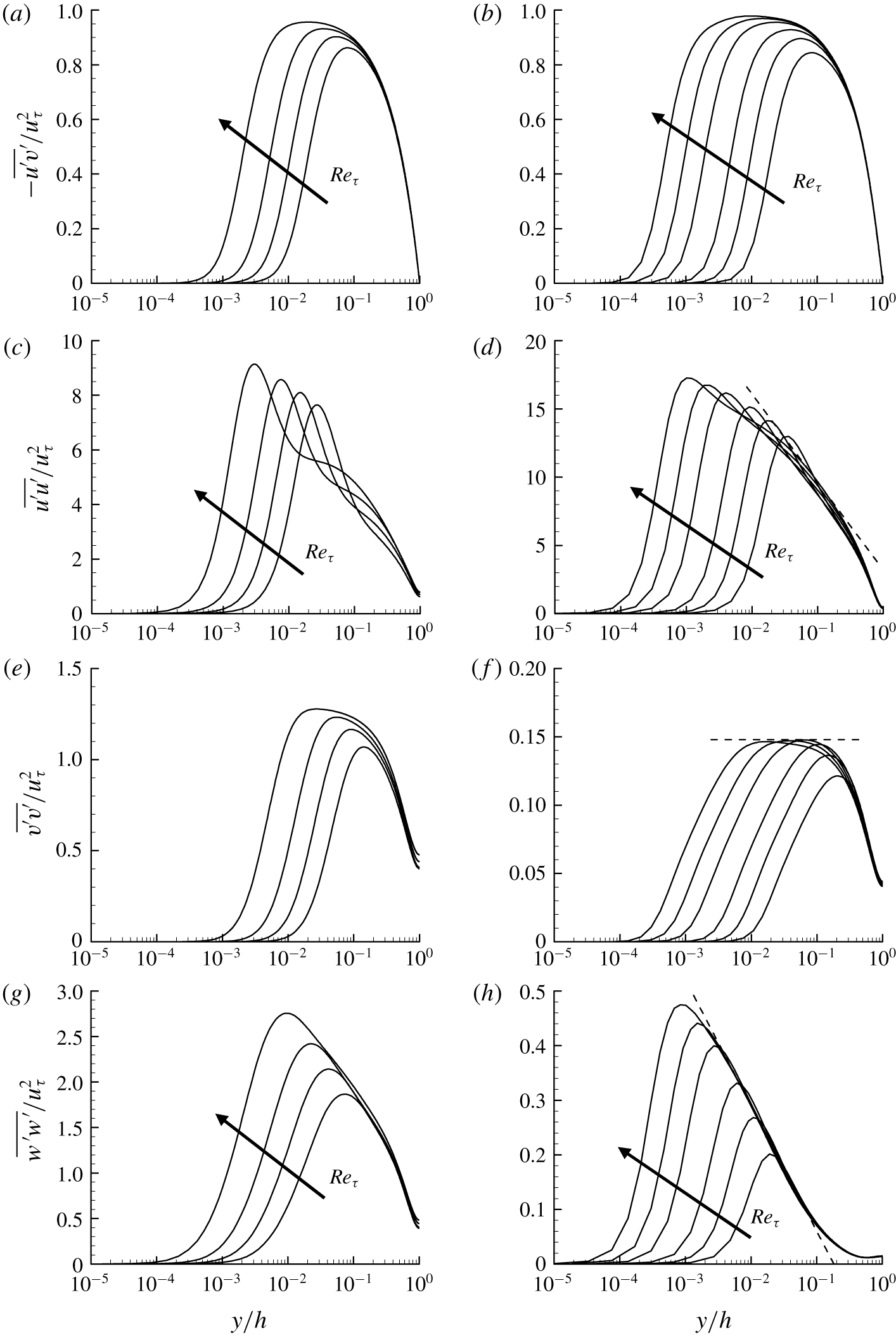
Reynolds-stress profile from (a,c,e,g) DNS (Lee & Moser Reference Lee and Moser2015) and (b,d,f,h) QLA ( $N_{POD}=2$) in the outer-scaled wall-normal coordinate: (a,b)
 $-\overline{u^{\prime }v^{\prime }}/u_{\unicode[STIX]{x1D70F}}^{2}$; (c,d)
 $\overline{u^{\prime }u^{\prime }}/u_{\unicode[STIX]{x1D70F}}^{2}$; (e,f)
 $\overline{v^{\prime }v^{\prime }}/u_{\unicode[STIX]{x1D70F}}^{2}$; (g,h)
 $\overline{w^{\prime }w^{\prime }}/u_{\unicode[STIX]{x1D70F}}^{2}$. Here,
 $Re_{\unicode[STIX]{x1D70F}}=543$, 1001, 1995, 5186 for DNS and
 $Re_{\unicode[STIX]{x1D70F}}=500$, 1000, 2000, 5000, 10 000, 20 000 for QLA. In (d,f,h), the dashed lines are the fits obtained at
 $Re_{\unicode[STIX]{x1D70F}}=20\,000$ using the theoretical result of Townsend (Reference Townsend1976) (see (3.1)).

As discussed in the previous section, the spectra of the present QLA for  $N_{POD}=2$ describe many important statistical features of energy-containing motions in DNS or real flow qualitatively well, except the one associated with the energy cascade. Using this observation, the QLA model is solved in a range of Reynolds numbers from
 $Re_{\unicode[STIX]{x1D70F}}=500$ to
 $Re_{\unicode[STIX]{x1D70F}}=20\,000$. The inner- and outer-scaled Reynolds-stress profiles of DNS (Lee & Moser Reference Lee and Moser2015) and the present QLA are then compared in figures 8 and 9, respectively. It appears that the scaling behaviour of the Reynolds-stress profiles of the QLA with Reynolds number is strikingly similar to that of DNS at lower Reynolds numbers (up to
 $Re_{\unicode[STIX]{x1D70F}}=5186$). Furthermore, on increasing Reynolds number up to
 $Re_{\unicode[STIX]{x1D70F}}=20\,000$, it becomes evident that the streamwise and spanwise turbulence intensities gradually exhibit the logarithmic wall-normal dependence (figure 9d,h), while the Reynolds shear stress and the wall-normal turbulence intensity show the region where their profiles are roughly constant in the wall-normal direction (figure 9b,f). This is consistent with the early theoretical prediction of Townsend (Reference Townsend1976) and Perry & Chong (Reference Perry and Chong1982). By trial and error, a good fit of their prediction to the Reynolds-stress profiles of the present QLA is obtained as
 $$\begin{eqnarray}\displaystyle & \displaystyle \frac{\overline{u^{\prime }u^{\prime }}}{u_{\unicode[STIX]{x1D70F}}^{2}}=-2.8\ln \left(\frac{y}{h}\right)+3.2, & \displaystyle\end{eqnarray}$$
 $$\begin{eqnarray}\displaystyle & \displaystyle \frac{\overline{v^{\prime }v^{\prime }}}{u_{\unicode[STIX]{x1D70F}}^{2}}=0.148, & \displaystyle\end{eqnarray}$$
 $$\begin{eqnarray}\displaystyle & \displaystyle \frac{\overline{w^{\prime }w^{\prime }}}{u_{\unicode[STIX]{x1D70F}}^{2}}=-0.1\ln \left(\frac{y}{h}\right)-0.17. & \displaystyle\end{eqnarray}$$
 $Re_{\unicode[STIX]{x1D70F}}\geqslant 5000$ (figure 9d,h), indicating a possibility for them to be Reynolds-number-independent constants. By contrary, the second constant on the right-hand side of (3.1a) does show a little dependence on the Reynolds number (figure 9d), although the one on the right-hand side of (3.1c) appears not to (figure 9h). Also, it needs to be mentioned that the constants in (3.1) should not be directly compared with those from DNS or from experimental data because their values would be directly affected by the quantitative detail of the spectral covariance matrix in (2.12). Finally, the streamwise turbulence intensity profile of the QLA reported in figure 9(d) does not appear to reproduce a plateau-like behaviour observed in the lower logarithmic region of DNS (figure 9c). This may well be due to the lack of the modes for
 $k_{x}\neq 0$ in the present model, implying that a more sophisticated effort needs to be made to retrieve this feature within the framework of the proposed QLA.
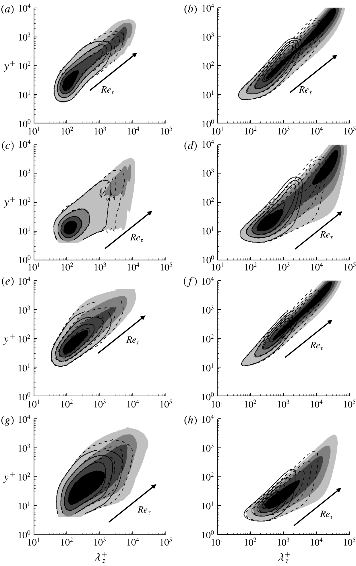
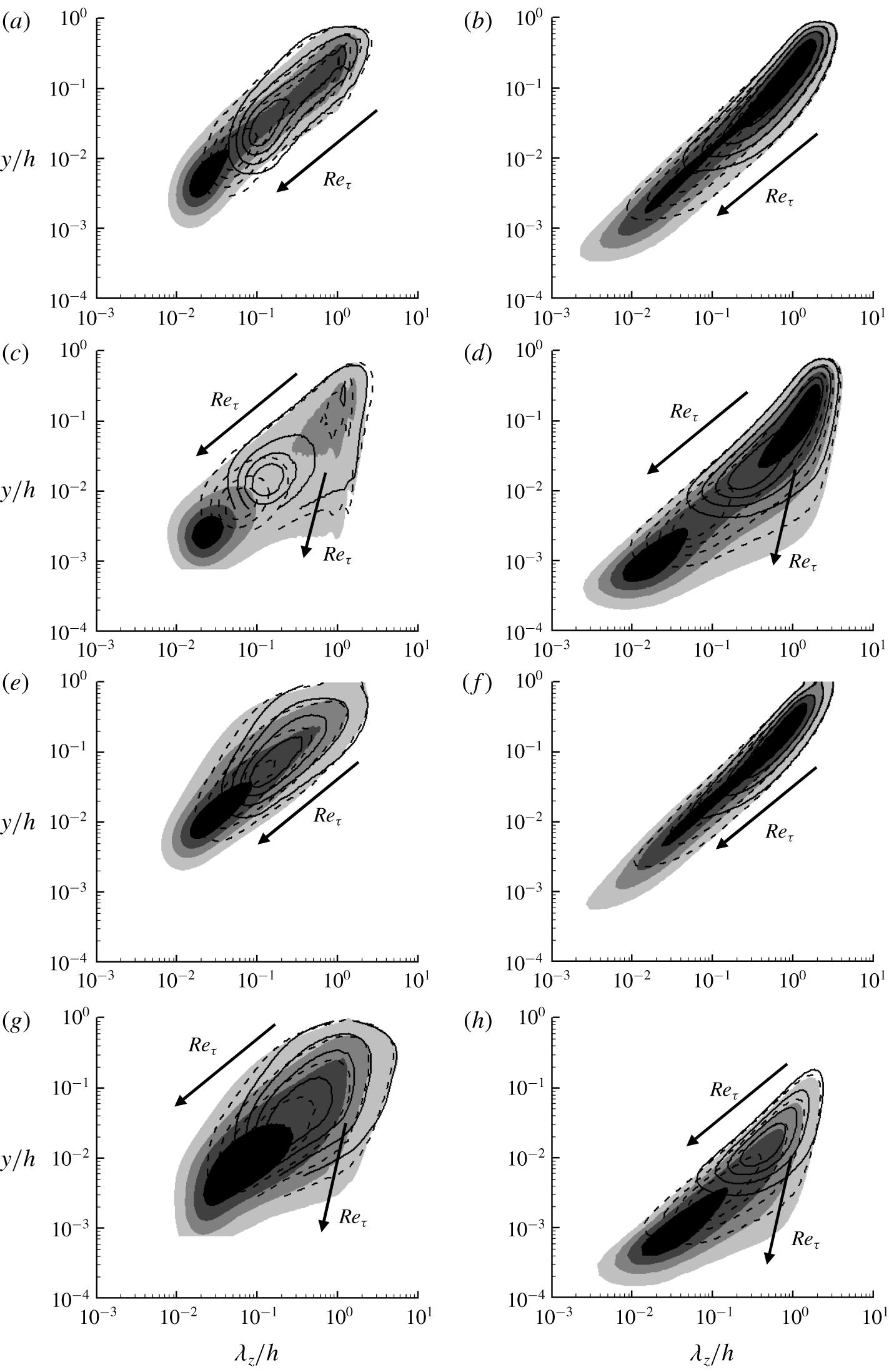
The inner- and outer-scaled spanwise wavenumber spectra of Reynolds stress from DNS and the present QLA are also compared in figures 10 and 11, respectively. As expected from figures 8 and 9, the spectra of the present QLA also exhibit exactly the same qualitative behaviour as those of DNS. All the spectra of the QLA span from  $\unicode[STIX]{x1D706}_{z}^{+}\simeq O(10)$ to
 $\unicode[STIX]{x1D706}_{z}\simeq O(h)$ like those of DNS. The near-wall part of the spectra of the QLA (say
 $y^{+}\leqslant O(100)$) scales very well in inner units for
 $\unicode[STIX]{x1D706}_{z}^{+}\leqslant O(100)$ like that of DNS (figure 8). The outer part of all the spectra for both DNS and QLA exhibits very good scaling in the outer region (figure 9), while the streamwise and spanwise velocity spectra develop a wall-reaching inactive part at large
 $\unicode[STIX]{x1D706}_{z}$ with increasing
 $Re$; for example, as
 $Re$ is increased, the lowest contour levels in figure 11(c,d,g,h) at large
 $\unicode[STIX]{x1D706}_{z}$ extend to the wall. We note that the development of the wall-reaching inactive part in each of these spectra is the crucial element for the streamwise and spanwise velocity fluctuations to have the logarithmic wall-normal dependence (Townsend Reference Townsend1976; Perry & Chong Reference Perry and Chong1982), consistent with the result shown in figures 8 and 9. Nevertheless, any firm evidence on
 $k_{z}^{-1}$ spectra does not seem to emerge even at
 $Re_{\unicode[STIX]{x1D70F}}=20\,000$ in the present QLA. This result is consistent with the previously reported experimental data (Samie et al. Reference Samie, Marusic, Hutchins, Fu, Fan, Hultmark and Smits2018; Baars & Marusic Reference Baars and Marusic2020a,Reference Baars and Marusicb), and it indicates that the computation at much higher Reynolds numbers would be needed for any firm conclusion on the emergence of
 $k_{z}^{-1}$ spectra.
Inner-scaled spanwise wavenumber spectra from (a,c,e,g) DNS (Lee & Moser Reference Lee and Moser2015; Hoyas & Jiménez Reference Hoyas and Jiménez2006) and (b,d,f,h) QLA ( $N_{POD}=2$): (a,b) Reynolds shear stress; (c,d) streamwise velocity; (e,f) wall-normal velocity; (g,h) spanwise velocity. Here,
 $Re_{\unicode[STIX]{x1D70F}}=934$, 2003, 5186 for DNS and
 $Re_{\unicode[STIX]{x1D70F}}=1000$, 5000, 20 000 for QLA. In (a,c,e,g), the solid-line, dashed-line and shaded contours indicate
 $Re_{\unicode[STIX]{x1D70F}}=934$, 2003, 5186, whereas in (b,d,f,h) they indicate
 $Re_{\unicode[STIX]{x1D70F}}=1000$, 5000, 20 000, respectively. The contour levels are chosen as 0.25, 0.5 and 0.75 times each of the maximum for comparison.

Outer-scaled spanwise wavenumber spectra from (a,c,e,g) DNS (Hoyas & Jiménez Reference Hoyas and Jiménez2006; Lee & Moser Reference Lee and Moser2015) and (b,d,f,h) QLA ( $N_{POD}=2$): (a,b) Reynolds shear stress; (c,d) streamwise velocity; (e,f) wall-normal velocity; (g,h) spanwise velocity. In (a,c,e,g) the solid-line, dashed-line and shaded contours indicate
 $Re_{\unicode[STIX]{x1D70F}}=934$, 2003, 5186, whereas in (b,d,f,h) they indicate
 $Re_{\unicode[STIX]{x1D70F}}=1000$, 5000, 20 000, respectively. The contour levels are chosen as 0.25, 0.5 and 0.75 times each of the maximum for comparison.

3.3 The near-wall peak in streamwise and spanwise turbulence intensities
Lastly, in this section, we provide one example of an open question that can be addressed within the proposed quasi-linear model. In particular, we will use the proposed quasi-linear approximation as a ‘predictive’ tool for the scaling behaviour of the near-wall peak turbulence intensity with Reynolds number. While the proposed quasi-linear approximation relies on a phenomenological minimal model for  ${\mathcal{N}}$ given in (2.2), it should be mentioned that the near-wall behaviour of the POD modes used here has been shown to behave very similarly to that of the near-wall velocity spectra (for a detailed discussion, see Hwang & Cossu (Reference Hwang and Cossu2010b), Hwang (Reference Hwang2016)). Therefore, we anticipate that this would be a useful exercise for the demonstration of the capability of the proposed quasi-linear model.
Early evidence at moderately high Reynolds numbers ( $Re_{\unicode[STIX]{x1D70F}}<10^{4}$) suggested that the peak streamwise turbulence intensity may grow logarithmically with the friction Reynolds number (see Marusic et al. Reference Marusic, McKeon, Monkewitz, Nagib, Smits and Sreenivasan2010). However, recent measurement of the near-wall region up to
 $Re_{\unicode[STIX]{x1D70F}}=4\times 10^{4}$ in the CICLoPE facility (Willert et al. Reference Willert, Soria, Stanislas, Klinner, Amili, Eisfelder, Cuvier, Bellani, Fiorini and Talamelli2017) suggested that the peak streamwise turbulence intensity may begin to deviate from the logarithmic scaling for
 $Re_{\unicode[STIX]{x1D70F}}\geqslant 10^{4}$. By contrary, the other recent measurement in the boundary layer (Samie et al. Reference Samie, Marusic, Hutchins, Fu, Fan, Hultmark and Smits2018) showed that the peak intensity may continue to follow the logarithmic scaling at least up to
 $Re_{\unicode[STIX]{x1D70F}}=2\times 10^{4}$. The logarithmic growth of the near-wall region has been believed to be important evidence supporting the attached eddy hypothesis, and it can be described with the following semi-empirical extension of the attached eddy model of Townsend (Reference Townsend1976) for the near-wall turbulence intensity (Marusic & Kunkel Reference Marusic and Kunkel2003):
 $$\begin{eqnarray}\frac{\overline{u^{\prime }u^{\prime }}}{u_{\unicode[STIX]{x1D70F}}^{2}}=f_{i}(y^{+})f_{T}(y^{+};Re_{\unicode[STIX]{x1D70F}}).\end{eqnarray}$$
Here  $f_{i}(y^{+})$ models the universal part of near-wall turbulence intensity and
 $$\begin{eqnarray}f_{T}(y^{+};Re_{\unicode[STIX]{x1D70F}})=1+(\unicode[STIX]{x1D6FC}-1)\frac{\ln (y^{+})}{\ln (y_{ref}^{+})},\end{eqnarray}$$
with
 $$\begin{eqnarray}\unicode[STIX]{x1D6FC}=\frac{B_{1}-A_{1}\ln (y^{+}/Re_{\unicode[STIX]{x1D70F}})}{B_{1}-A_{1}\ln (y_{ref}^{+}/Re_{\unicode[STIX]{x1D70F},ref})}\end{eqnarray}$$
describing the near-wall influence of the energy-containing motions in the logarithmic and outer regions. Here,  $A_{1}$ and
 $B_{1}$ are the constants emerging in the original model of Townsend (Reference Townsend1976) for the logarithmic layer,
 $y_{ref}^{+}$ and
 $Re_{\unicode[STIX]{x1D70F},ref}$ are the reference inner-scaled wall-normal location and friction Reynolds number, respectively; for example,
 $y_{ref}^{+}=50$ and
 $Re_{\unicode[STIX]{x1D70F},ref}=2000$ were chosen in Marusic & Kunkel (Reference Marusic and Kunkel2003). In this model, if the peak wall-normal location is assumed to scale in inner units (i.e.
 $y_{max}^{+}=\text{const.}$),
 $\overline{u^{\prime }u^{\prime }}/u_{\unicode[STIX]{x1D70F}}^{2}\sim \ln Re_{\unicode[STIX]{x1D70F}}$ is obtained – in fact, (3.2) gives a logarithmic growth of the near-wall streamwise turbulence intensity with
 $Re_{\unicode[STIX]{x1D70F}}$ whenever the wall-normal location is chosen to scale in inner units.
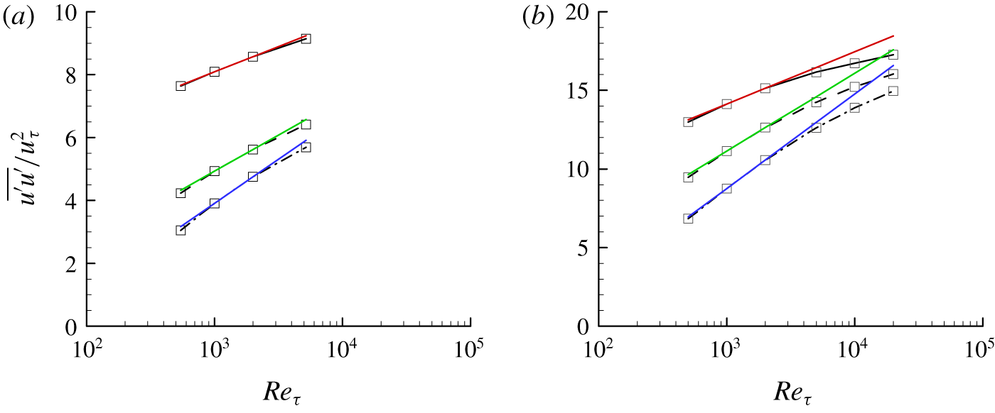
To gain a physical insight into the scaling of the peak streamwise turbulence intensity with  $Re_{\unicode[STIX]{x1D70F}}$, the streamwise turbulence intensities of DNS and QLA at three different wall-normal locations (
 $y^{+}=y_{max}^{+},50,100$, where
 $y_{max}$ is the peak wall-normal location) are shown in figure 12. Here, the data are presented with the fits given in the form of
 $\overline{u^{\prime }u^{\prime }}/u_{\unicode[STIX]{x1D70F}}^{2}=a+b\ln Re_{\unicode[STIX]{x1D70F}}$, where the constants
 $a$ and
 $b$ are obtained from the data at
 $Re_{\unicode[STIX]{x1D70F}}=1000,2000$. The streamwise turbulence intensity of DNS at
 $y^{+}=y_{max}^{+}$ appears to grow logarithmically with
 $Re_{\unicode[STIX]{x1D70F}}$ at least up to
 $Re_{\unicode[STIX]{x1D70F}}\simeq 5000$, as reported by Lee & Moser (Reference Lee and Moser2015) (figure 12a). The peak intensities of QLA also seem to behave like those of DNS for
 $Re_{\unicode[STIX]{x1D70F}}\leqslant 5000$ (figure 12b). However, a closer look suggests that the peak streamwise turbulence intensity from both DNS and QLA for
 $Re_{\unicode[STIX]{x1D70F}}\leqslant 5000$ very slightly deviate from the logarithmic scaling obtained at
 $Re_{\unicode[STIX]{x1D70F}}=1000,2000$. If the Reynolds number is further increased, it becomes evident that the data from the present QLA show a non-negligible deviation from the logarithmic scaling with
 $Re_{\unicode[STIX]{x1D70F}}$. To check this observation more carefully, the data of DNS and QLA are further examined at the other two inner-scaling wall-normal locations (
 $y^{+}=50,100$). In this case, even the DNS data for
 $Re_{\unicode[STIX]{x1D70F}}\leqslant 5186$ show rather visible deviations from logarithmic scalings (figure 12a), and the same behaviour is more clearly observed in the QLA data obtained up to
 $Re_{\unicode[STIX]{x1D70F}}=20\,000$ (figure 12b).
Growth of the peak streamwise turbulence intensity with  $Re_{\unicode[STIX]{x1D70F}}$: (a) DNS at
 $Re_{\unicode[STIX]{x1D70F}}=543$, 1001, 1995, 5186 (Lee & Moser Reference Lee and Moser2015); (b) QLA at
 $Re_{\unicode[STIX]{x1D70F}}=500$, 1000, 2000, 5000, 10 000, 20 000. Here, ——,
 $y^{+}=y_{max}^{+}$; – – – –,
 $y^{+}=50$; – ⋅ – ⋅ –,
 $y^{+}=100$. Each of the coloured straight lines indicates the fit given in the form of
 $\overline{u^{\prime }u^{\prime }}/u_{\unicode[STIX]{x1D70F}}^{2}=a+b\ln Re_{\unicode[STIX]{x1D70F}}$, where the constants
 $a$ and
 $b$ are obtained from the data at
 $Re_{\unicode[STIX]{x1D70F}}=1000,2000$.

The only possible explanation for this deviation from the logarithmic scaling would be that the extent that each of the relatively large energy-containing motions in the logarithmic and outer regions influences the near-wall region is slightly reduced as  $Re_{\unicode[STIX]{x1D70F}}$ increases – if not, it is not possible to explain why the near-wall spectra of DNS and QLA at small
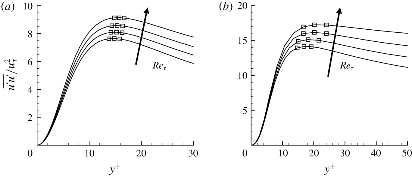
 $\unicode[STIX]{x1D706}_{z}$ scale so well in inner units (figure 10c,d). Further supporting evidence on this argument can be found in figure 13, where the peak wall-normal locations of the streamwise turbulence intensity of DNS and QLA are shown to slightly move away from the wall on increasing
 $Re_{\unicode[STIX]{x1D70F}}$. This observation implies that the prediction by the model (3.2) would actually have a small deviation from the behaviour of the DNS and QLA data (figures 12 and 13), as the peak wall-normal locations do not precisely scale in inner units (figure 13).
Near-wall streamwise turbulence intensity: (a) DNS at  $Re_{\unicode[STIX]{x1D70F}}=543$, 1001, 1995, 5186 (Lee & Moser Reference Lee and Moser2015); (b) QLA at
 $Re_{\unicode[STIX]{x1D70F}}=1000$, 2000, 5000, 20 000. Here, the symbols indicate the locations of the three grid points around the maximum of each curve.

The discussion here appears to favour the conclusion of Willert et al. (Reference Willert, Soria, Stanislas, Klinner, Amili, Eisfelder, Cuvier, Bellani, Fiorini and Talamelli2017), but it is not necessarily against the one of Samie et al. (Reference Samie, Marusic, Hutchins, Fu, Fan, Hultmark and Smits2018) made in the boundary layer. We note that the spanwise length scale of the large-scale outer structures in the boundary layer (i.e. large-scale and very large-scale motions) is  $\unicode[STIX]{x1D706}_{z}\simeq 0.8\unicode[STIX]{x1D6FF}_{99}$ (
 $\unicode[STIX]{x1D6FF}_{99}$ is the thickness of the boundary layer), a little smaller than
 $\unicode[STIX]{x1D706}_{z}\simeq 1.4R$ in pipe flow (
 $R$ is the pipe radius). Therefore, their highest Reynolds number (
 $Re_{\unicode[STIX]{x1D70F}}\simeq 20\,000$) might have not been high enough to see a rather clear deviation from the logarithmic scaling with
 $Re_{\unicode[STIX]{x1D70F}}$. Finally, it should be mentioned that the discussion given here applies to the scaling of the peak spanwise turbulence intensity in exactly the same manner, thus, it is not repeated.
4 Concluding remarks
In the present study, a quasi-linear description of the Navier–Stokes equations for first- and second-order turbulence statistics have been proposed for parallel wall-bounded shear flows. The velocity field is decomposed into a mean and fluctuations. While the mean is obtained from the full nonlinear equation (2.1a), the fluctuation equations are linearised by replacing the nonlinear self-interaction terms with a simple model composed of an eddy-viscosity-based turbulent diffusion and a stochastic forcing. Under this particular setting, the fluctuation equations are linear, enabling superposition of their solutions for the construction of Reynolds stress. This feature is compatible to the essential elements of the classical attached eddy model. Based on this framework, the colour in the spanwise direction and amplitude of the stochastic forcing have been determined self-consistently by solving an optimisation problem which minimises the difference between the Reynolds shear stresses from the mean and fluctuations with a constraint that the averaged spectrum of the forcing must be sufficiently smooth in Fourier space. The proposed quasi-linear approximation has subsequently been applied to turbulent channel flow for friction Reynolds numbers ranging from  $Re_{\unicode[STIX]{x1D70F}}=500$ to
 $Re_{\unicode[STIX]{x1D70F}}=20\,000$. The best result is obtained when the Reynolds stress is constructed using only the two leading POD modes, a procedure that evidently filters out the modelling artefact caused by the unphysical stochastic forcing. In this case, it has been shown that the resulting turbulence intensity profile and energy spectra exhibit exactly the same qualitative behaviour as DNS data throughout the entire wall-normal location, reproducing the early theoretical predictions of Townsend and Perry within a controlled approximation to the Navier–Stokes equation. Finally, the proposed quasi-linear approximation has shown that the peak streamwise and spanwise turbulence intensities can slightly deviate from the logarithmic scaling with
 $Re_{\unicode[STIX]{x1D70F}}$, and the supporting evidence from the existing DNS data has also been presented.
The proposed QLA is evidently an extension of the early quasi-linear framework of Malkus (Reference Malkus1956) and Herring (Reference Herring1963) to a linearly stable turbulent shear flow at high Reynolds numbers, where the classical marginal stability criterion is not applicable. For this purpose, stochastically driven linearised fluctuation equations are self-consistently obtained only with minimal statistical information (i.e. mean velocity) and with a minimal physical model for the self-interacting nonlinear terms in the fluctuation equations. The design procedure of the stochastic linearised fluctuation equations shares exactly the same idea with the attached eddy model of Townsend (Reference Townsend1976) and Perry & Chong (Reference Perry and Chong1982), i.e. the self-similar POD modes from the stochastically driven linear system are suitably superposed to generate the Reynolds shear stress of the mean equation. In the context of the stochastically driven linearised Navier–Stokes system, Jovanović & Bamieh (Reference Jovanović and Bamieh2001) empirically designed the wall-normal profile of stochastic forcing to improve its response in comparison to the turbulence statistics from DNS. However, in many senses, the proposed quasi-linear framework shares more similarities with the recent work of Zare, Jovanović & Georgiou (Reference Zare, Jovanović and Georgiou2017), where the unknown turbulence statistics (i.e. full information of spectral covariance matrix) are recovered by suitably designing stochastic linearised fluctuation equations using the ‘known’ statistics (power and cross-spectral densities of DNS). Indeed, Zare et al. (Reference Zare, Jovanović and Georgiou2017) determined the colour of the stochastic forcing for the purpose of seeking a more accurate data-driven model of the nonlinearity. However, it is worth pointing out that the power and cross-spectral densities used as the ‘inputs’ in their study are often the ultimate statistical ‘outputs’ of interest in many cases, because they can only be obtained with DNS or accurate laboratory experiment. By contrast, the proposed framework requires only mean velocity, and it produces the related second-order statistics and spanwise wavenumber spectra in qualitative agreement with those of DNS. In other words, provided the mean velocity is available, the proposed quasi-linear model would be a useful framework to study the scaling of second-order turbulence statistics with its ‘predictive’ nature for the certain statistical properties of interest.
Acknowledgements
While this paper was being drafted, Professor B. Eckhardt (B.E.) passed away unexpectedly. This work was started in September, 2017, when B.E. introduced quasi-linear approximation to Y.H. (Pausch et al. Reference Pausch, Yang, Hwang and Eckhardt2019). Since then, Y.H. has been greatly privileged by many illuminating discussions with B.E. not only on the subject of this work but also on the other scientific subjects such as active fluids. It has been with great sadness to complete this paper without B.E. His sharp scientific mind and many helpful advices will be remembered and very much missed for a long time.
Y.H. gratefully acknowledges the partial support of the Leverhulme Trust (RPG-2019-123) and thanks Professor M. Jovanović for some useful suggestions for the original manuscript.
Declaration of interests
The authors report no conflict of interest.
Appendix. Sensitivity to the optimisation parameters
In this section, sensitivity of the optimisation problem in § 2.3 to the parameter  $\unicode[STIX]{x1D701}$ for
 $\boldsymbol{M}$ and the integration weight
 $Q(y)=(1-y/h)^{m}$ (
 $m$ is a positive real number) in (2.16) is studied. In figure 14 we show how the solution to the optimisation problem
 $W(k_{z})$ is changed with respect to
 $\unicode[STIX]{x1D701}$. Given the form of
 $\boldsymbol{M}(=\text{diag}[\text{e}^{\unicode[STIX]{x1D701}}~\text{e}^{2\unicode[STIX]{x1D701}}~\text{e}^{3\unicode[STIX]{x1D701}}\ldots \text{e}^{N_{\unicode[STIX]{x1D6FD}}\unicode[STIX]{x1D701}}])$, it is evident that a low value of
 $\unicode[STIX]{x1D701}$ would allow
 $W(k_{z})$ to take a more complicated form, whereas a high value of
 $\unicode[STIX]{x1D701}$ would restrict it to be a highly smooth function. This is exactly seen in figure 14(a) where
 $W(k_{z})$ is plotted for
 $\unicode[STIX]{x1D701}=0.1$, 0.3, 0.5, 0.7, 0.9, 1.1, although the overall shape of
 $W(k_{z})$ remains to be changed only a little. Given the role of
 $\unicode[STIX]{x1D701}$, it is also expected that the difference between the Reynolds shear stresses from the mean equation and the fluctuations equations with the computed
 $W(k_{z})$ would increase with
 $\unicode[STIX]{x1D701}$. Indeed, the two measures quantifying the Reynolds-shear-stress difference (i.e.
 $\unicode[STIX]{x1D716}_{1}=\Vert \overline{u^{\prime }v^{\prime }}-\langle u^{\prime }v^{\prime }\rangle \Vert _{Q}^{2}$ and
 $\unicode[STIX]{x1D716}_{2}=\Vert \overline{u^{\prime }v^{\prime }}-\langle u^{\prime }v^{\prime }\rangle \Vert _{L_{2}}^{2}$) do increase with
 $\unicode[STIX]{x1D701}$, as shown in figure 14(b). In particular, it appears that
 $\unicode[STIX]{x1D716}_{1}\leqslant 10^{-6}$ and
 $\unicode[STIX]{x1D716}_{2}\leqslant 10^{-4}$ if
 $\unicode[STIX]{x1D701}\leqslant 0.5$ is chosen. Therefore, to obtain a reasonable degree of freedom for the shape of
 $W(k_{z})$ and sufficiently low
 $\unicode[STIX]{x1D716}_{1}$ and
 $\unicode[STIX]{x1D716}_{2}$,
 $\unicode[STIX]{x1D701}=0.5$ is chosen in the present study.
Sensitivity of the optimisation problem (2.16) and (2.17) to the smoothness control parameter  $\unicode[STIX]{x1D701}$: (a)
 $W(k_{z})$; (b) optimisation errors with
 $\unicode[STIX]{x1D701}$, where
 $\unicode[STIX]{x1D716}_{1}=\Vert \overline{u^{\prime }v^{\prime }}-\langle u^{\prime }v^{\prime }\rangle \Vert _{Q}^{2}$ (○) and
 $\unicode[STIX]{x1D716}_{2}=\Vert \overline{u^{\prime }v^{\prime }}-\langle u^{\prime }v^{\prime }\rangle \Vert _{L_{2}}^{2}$ (▫). Here, ——,
 $\unicode[STIX]{x1D701}=0.1$; – – – –,
 $\unicode[STIX]{x1D701}=0.3$; – ⋅ – ⋅ –,
 $\unicode[STIX]{x1D701}=0.5$;
 $\cdots \cdots$,
 $\unicode[STIX]{x1D701}=0.7$; — —,
 $\unicode[STIX]{x1D701}=0.9$; – ⋅⋅ – ⋅⋅ –,
 $\unicode[STIX]{x1D701}=1.1$.

Sensitivity of the optimisation (2.16) and (2.17) to the integration weight  $Q(y)=(y/h-1)^{m}$ with
 $m=0$, 2, 4, 6, 8, 10: (a)
 $W(k_{z})$; (b) optimisation errors with
 $m$, where
 $\unicode[STIX]{x1D716}_{1}=\Vert \overline{u^{\prime }v^{\prime }}-\langle u^{\prime }v^{\prime }\rangle \Vert _{Q}^{2}$ (○) and
 $\unicode[STIX]{x1D716}_{2}=\Vert \overline{u^{\prime }v^{\prime }}-\langle u^{\prime }v^{\prime }\rangle \Vert _{L_{2}}^{2}$ (▫). Here, ——,
 $m=0$; – – – –,
 $m=2$; – ⋅ – ⋅ –,
 $m=4$;
 $\cdots \cdots$,
 $m=6$; — —,
 $m=8$; – ⋅⋅ – ⋅⋅ –,
 $m=10$.

Sensitivity to the choice of the integration weight  $Q(y)=(1-y/h)^{m}$ is also studied by considering
 $0\leqslant m\leqslant 1$. In figure 15 we show the solution to the optimisation problem (
 $W(k_{z})$) and the two measures quantifying the Reynolds-shear-stress difference (
 $\unicode[STIX]{x1D716}_{1}$ and
 $\unicode[STIX]{x1D716}_{2}$). It appears that
 $W(k_{z})$ changes rather insensitively to the choice of
 $m$ (figure 15a). This is also seen in the values of
 $\unicode[STIX]{x1D716}_{1}$ and
 $\unicode[STIX]{x1D716}_{2}$ for
 $m$ considered. As long as
 $m\geqslant 8$,
 $\unicode[STIX]{x1D716}_{1}\leqslant 10^{-6}$ and
 $\unicode[STIX]{x1D716}_{2}\leqslant 10^{-4}$ (figure 15b). In particular, the lowest
 $\unicode[STIX]{x1D716}_{1}$ (the quantity identical to the objective functional in (2.17) is obtained when
 $m=6$. Therefore,
 $m=6$ is chosen for the integration weight
 $Q(y)$ in (2.16) and (2.17) throughout the present study.