NOMENCLATURE
- HE
Heading Error
- PN
Proportional Navigation
- LOS
Line of Sight
- FOV
Field of View
- SINS
Strap-down Inertial Navigation System
- A, B, D
state (system) matrix, control (input) matrix, and disturbance matrix
- b, c
penalties imposed by the miss distance and the terminal normal velocity
- Bk
discrete control (input) matrix
- g
gravitational acceleration, ms–2
- g 1, g 2, g 3
optimal guidance law gains
- H
measurement matrix
- J
optimal control performance index
- K 1, K 2, Kk
Kalman gains
- Mk
covariance matrix
- N
navigation constant
- nk
achieved missile lateral acceleration
- Pk
covariance matrix
- P0
initial covariance matrix
- Qk
process noise matrix
- r
range, m
- R
measurement noise matrix
- Rk
covariance matrix
- uk
guidance law
- t
time, s
- t f
time final, s
- T s
simple time, s
- t go
time to go, s
- u, w
lateral accelerations, ms–2
- V c
closing velocity, ms–1
- vk
noise measurement vector
- w 0
target manoeuvre, ms–2
- x
state-space vector
- x0
initial distance, m
- x 1, x 2
lateral relative displacement and relative velocity, m, ms–2
- x*1k
pseudo-measurement of relative position
 ${\hat{x}_{1k}}$, ${\hat{x}_{2k}}$
estimated values of the state vector elements.
- z0
initial height, m
- Zk
measurement vector
- Φ
continuous transition matrix
- Φk
discrete transition matrix
- Φs
spectral density
- λ
angle of line of sight rad
- $\mathop \lambda \limits^\centerdot $,λ1,λ2
lOS rate
- λ*k
measured LOS
- η
demand fin deflection
- ηM
achieved lateral acceleration
- ηc
achieved fin deflection
- σn
variance of the measurement noise
- σλ
Gaussian noise, mrad


1.0 INTRODUCTION
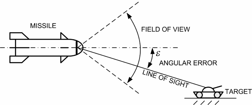
The precision guided expensive weapon plays a more and more important role in the modern war, so the development of missile guidance has become the focus of world militaries (see Reference Delong, Suochang and YingxiRef. 1). Accuracy and precision of simple aerial bombs can be significantly improved by using the simple target tracking device and actuators for aerodynamic control surfaces. The Proportional Navigation (PN) is one of the commonly used guidance laws in practice. This law was used extensively in short and medium range homing missile guidance and control systems (see Reference Yao, Wei Zhou and WangRefs 2 and Reference David and Solomon3). Trajectory tracking guidance laws presented in Reference Pavkovic, Pavic and CukRef. 4 were not suitable for homing, and only the pulse frequency modulation could be adopted. In the case of slowly manoeuvring ground targets, in Reference Kun, Chiang and ChenRef. 5, the pursuit guidance law was used as a guidance approach where the velocity vector always points to a target. The use of the pursuit guidance law implies attaching a statically stable aerodynamic sensor platform on the top of the aerial bomb, which always positions itself in the direction of the velocity vector. Laser seeker on this platform detects the angular deviation of the Line of Sight (LOS) from the velocity direction, and this information is used to calculate steering commands for trajectory correction. If the applied seeker has a large enough Field of View (FOV), it can be directly mounted on the top of the bomb, as shown in Fig. 1.
Strap-down (non-gimballed) homing head.

In this way, this bomb does not require any gimballed tracking system part, but only a strap-down seeker system which is defined in Reference Dowan, Chang-Kyung, Yongho and JongjuRef. 6. Besides the seeker, the system must include a Strap-down Inertial Navigation System (SINS), see Reference Jwo, Shih, Hsu and YuRef. 7, with solid-state components and three rate gyroscopes. This system is mechanically less complex and more reliable. Such a system allows us to detect an angular deviation of LOS relative to the body-fixed coordinate frame and it cannot measure LOS rate ( $\mathop \lambda \limits^\centerdot $). However, it gives information on the angle between the LOS and the centreline of the missile (ε). This information is used as the error input in the guidance loop. In Reference Sun, Chu, Zhang, Jia, Guo, Zhang and ZhangRefs 8 and Reference Tapas, Rao and Prabhakar9, a Kalman filter is used to eliminate noise from the measured LOS rate. In this paper, we used the Kalman filter to estimate the LOS rate, based only on the measurement of the angular error (corrupted with noise), because the major problem is lack of information on the LOS rate as guidance laws based on PN or optimal guidance require this rate as the input value.
The objective of this work is to obtain a low cost and efficient guidance system that would be used on short-range guided bomb. In this paper, an optimal guidance method is proposed, based on a strap down seeker system. This system allows the detection of the angle between the LOS and the centreline of the missile, while in the pursuit guidance system it is relative to the velocity vector. This angle (ε) was used as an input to the Kalman filter for noise removal from the measured signals and for estimating the LOS rate (Reference Sun, Chu, Zhang, Jia, Guo, Zhang and ZhangRef. 8). This value is required for optimal guidance. Finally, after signal filtration, estimation and guidance control calculation, the coordinate transformation is used in the opposite direction, from guidance to body reference system, where commands are executed.
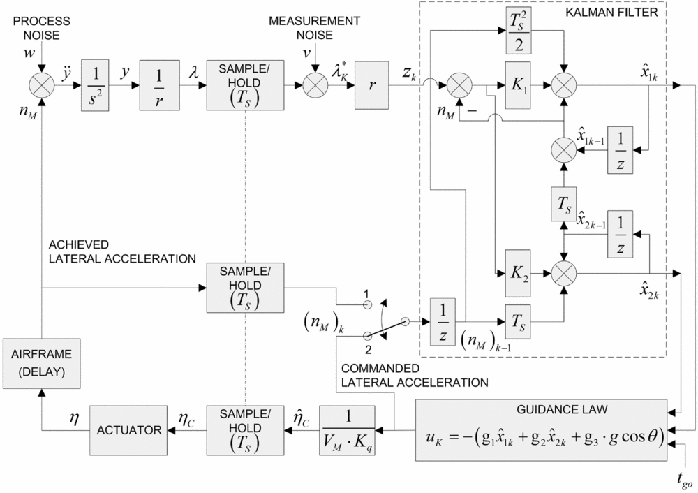
This paper is organised as follows. Section 2 presents the general theoretical basics of linear quadratic differential games (LQDG) and their application in the algorithm of optimal guidance law. In Section 3, the model of Kalman filter is used to eliminate noise from the measured signals and to estimate the LOS rate. The estimation of LOS rate, which is affected by the angle error, is needed for the optimal guidance law, which is shown in Fig. 2. In Section 4, the simulation results (lateral displacement, lateral velocity, trajectories, commanded lateral acceleration, terminal miss distance and deviation with different heading error) and the comparison with the different guidance methods are shown. Finally, Section 5 is devoted to the conclusions.
Second-order Kalman filter with position measurement only.

2.0 OPTIMAL GUIDANCE
The motion of the missile-target system in one plane is described by the following differential equation in state space (Reference Ben-AsherRef. 10):
 $$\begin{eqnarray}
\begin{array}{@{}c@{}} {{\bf \dot{x}}} = {{\bf Ax}} + {{\bf B}}u + {{\bf D}}w\\ {{\bf x}}({t_0}) = {\left[ {\begin{array}{*{20}{c}} {{x_{1}}({t_0})}&{{x_2}({t_0})} \end{array}\,} \right]^{{\mathop{\rm T}\nolimits} }}\\[6pt] {{\bf A}} = \left[ {\begin{array}{@{}*{2}{c}@{}} 0&1\\ 0&0 \end{array}} \right],\quad {{\bf B}} = \left[ {\begin{array}{@{}*{1}{c}@{}} 0\\ 1 \end{array}} \right],\quad {{\bf D}} = \left[ {\begin{array}{@{}*{1}{c}@{}} 0\\ 1 \end{array}} \right] \end{array}
\end{eqnarray}$$
Scalar variables x1 and x2 are the components of the state vector x, which also represent the relative lateral displacement and the velocity, respectively, while u and w are the corresponding lateral accelerations of the bomb and the target.
As shown in Reference Ben-AsherRef. 10, the optimal guidance problem is to minimise the following performance index:
 $$\begin{equation}
J = \frac{b}{2}x_{1}^2({t_{\rm{f}}}) + \frac{c}{2}x_2^2({t_{\rm{f}}}) + \frac{1}{2}\int\limits_{{{t_0}}}^{{{t_{\rm{f}}}}}{{{u^2}(t){\mathop{\rm d}\nolimits} t}}
\end{equation}$$
In the previous equation, b > 0 is a penalty imposed by the miss distance (i.e. the relative separation at the final time t f); the coefficient c > 0 is introduced to minimise the terminal lateral velocity. In the case when c < 0, the bomb's objective is to maximise the velocity. The last component represents command during the flight, and minimises it.
For the perfect interception, x 1(t f) = 0, it is required that b → ∞, and for the perfect rendezvous, besides the previous condition, there is also x 2(t f) = 0, and it is required that both penalty coefficients tend to infinity, i.e. b → ∞, c → ∞.
Assuming the target is manoeuvring with a constant lateral acceleration (w = const = w 0) starting at t = t 0, the expression of guidance control value was obtained in Reference Ben-AsherRef. 10, as the solution of a two-point boundary value, applying the given boundary conditions. These values are obtained by the following steps.
In the case of Performance index (Reference Yao, Wei Zhou and Wang2) minimising, the adjoin equations are:
 $$\begin{equation}
{\dot{\lambda }_{1}} = 0,\quad {\dot{\lambda }_{2}} = - {\lambda _{1}},\quad u = - {\lambda _{2}}
\end{equation}$$
 $$\begin{equation}
{\lambda _{1}}({t_{\rm{f}}}) = b{x_{1}}({t_{\rm{f}}}),\quad {\lambda _{2}}({t_{\rm{f}}}) = c{x_2}({t_{\rm{f}}})
\end{equation}$$
Solving these two equations gives:
 $$\begin{eqnarray}
{\lambda _{1}} &=& b{x_{1}}({t_{\rm{f}}}),\nonumber\\
{\lambda _{2}} &=& b{x_{1}}({t_{\rm{f}}})({t_{\rm{f}}} - t) + c{x_2}({t_{\rm{f}}})
\end{eqnarray}$$
And the control is:
 $$\begin{equation}
u(t) = - \left[ {b{x_{1}}({t_{\rm{f}}})({t_{\rm{f}}} - t) + c{x_2}({t_{\rm{f}}})} \right]
\end{equation}$$
Now, combining Equations (6) and (1), the expressions for x 1(t) and x 2(t) are obtained after integration from t 0 to t. After introducing the shift t = t f, the unknown final values x 1(t f) and x 2(t f) are solved, and finally the control law in closed form was determined as:
 $$\begin{eqnarray}
u\left( t \right) &=& - \left[ {{g_1}{x_{1}}(t) + {g_2}{x_2}(t) + {g_3}{w_0}} \right]\nonumber\\
{g_1} &=& \displaystyle\frac{{{t_{{\rm{go}}}}b\left( {\frac{1}{2}{t_{{\rm{go}}}}c + 1} \right)}}{{t_{{\rm{go}}}^4\frac{{cb}}{{12}} + t_{{\rm{go}}}^3\frac{b}{3} + {t_{{\rm{go}}}}c + 1}}\nonumber\\
{g_2} &=& \displaystyle\frac{{t_{{\rm{go}}}^3\frac{{cb}}{3} + t_{{\rm{go}}}^2b + c}}{{t_{{\rm{go}}}^4\frac{{cb}}{{12}} + t_{{\rm{go}}}^3\frac{b}{3} + {t_{{\rm{go}}}}c + 1}}\nonumber\\
{g_3} &=& \displaystyle\frac{{t_{{\rm{go}}}^4\frac{{cb}}{{12}} + t_{{\rm{go}}}^3\frac{b}{2} + {t_{{\rm{go}}}}c}}{{t_{{\rm{go}}}^4\frac{{cb}}{{12}} + t_{{\rm{go}}}^3\frac{b}{3} + {t_{{\rm{go}}}}c + 1}}
\end{eqnarray}$$
In the previous equations, t go = t f − t is the time-to-go (remaining time until impact).
Now, it is considered the so-called “perfect rendezvous,” where both the miss distance and the terminal velocity are minimised. In this case, from Equation (7) taking b → ∞ and c → ∞, feedback gains are obtained as:
 $$\begin{equation}
{g_{\rm{1}}} = \frac{6}{{t_{{\rm{go}}}^2}},\quad {g_{\rm{2}}} = \frac{4}{{{t_{{\rm{go}}}}}},\quad {g_{\rm{3}}} = 1
\end{equation}$$
The control signal can be expressed as:
 $$\begin{equation}
u = - {V_{\rm{c}}}\left( {4\dot{\lambda } + \frac{2}{{{t_{{\rm{go}}}}}}\lambda } \right) - {w_0},
\end{equation}$$
where V c is the closing velocity. The previous equation represents optimal guidance with navigation constant N = 4 and an additional feedback from the LOS angle, also with compensation factor 1 × w 0 to cancel out the target acceleration effect by performing exactly the opposite manoeuvre. For slowly moving objects on the ground, gravity is modelled as effective target acceleration and, thus, known in advance. In this way, the gravity influence in the vertical plane is compensated.
3.0 EXTENDED KALMAN FILTER
The continuous fundamental matrix (continuous transition matrix) is obtained from the system matrix (Reference Grewal and AndrewsRefs 11 and Reference Zarchan12):
 $$\begin{equation}
F(t) = {{\cal L}^{ - 1}}\{ {(s{{\bf I}} - {{\bf A}})^{ - 1}}\} = \left[ {\begin{array}{@{}*{2}{c}@{}} 1&t\\ 0&1 \end{array}} \right]
\end{equation}$$
Now, the discrete fundamental matrix (discrete transition matrix) can easily be found simply by replacing the continuous time with a sampling time:
 $$\begin{equation}
{\Phi _k} = \left[ {\begin{array}{@{}*{2}{c}@{}} 1&{{T_{\rm{s}}}}\\ 0&1 \end{array}} \right]
\end{equation}$$
The laser coordinator measures the LOS angle, and then a pseudo-measurement of relative position x*1k is created by multiplication of the LOS measurement by the range from missile to target:
 $$\begin{equation}
x_{1k}^ * = \lambda _{k}^ * r
\end{equation}$$
 $$\begin{equation}
{{{\bf z}}_k} = {{\bf H}}{{{\bf x}}_k} + {{{\bf v}}_k} = \left[ {\begin{array}{*{20}{c}} 1&0 \end{array}} \right]\left[ {\begin{array}{@{}*{1}{c}@{}} {{x_{1k}}}\\ {{x_{2k}}} \end{array}} \right] + {{{\bf v}}_k} = {x_{1k}} + {{{\bf v}}_k},
\end{equation}$$
where zk is the measurement vector (in our case, it is a scalar), H is the measurement matrix, and vk is the noise measurement vector (which is also a scalar). Noise measurement is assumed to be zero mean Gaussian noise and the noise measurement matrix R is related to the noise measurement vector according to 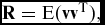 ${{\bf R}} = {\mathop{\rm E}\nolimits} ({{\bf v}}{{{\bf v}}^{\rm{T}}}),$ as mathematical expectation
 ${\mathop{\rm E}\nolimits} ( \cdot ),$ and in this case, it is a scalar value Rk = σ2n, where σ2n is the variance of the measurement noise.
The discrete form of control matrix is obtained from:
 $$\begin{equation}
{{{\bf B}}_k} = \int\limits_{0}^{{{T_{\rm{s}}}}}{{\Phi(t){{\bf B}}(t){\mathop{\rm d}\nolimits} t}} = \left[ {\begin{array}{@{}*{1}{c}@{}} {\displaystyle\frac{{T_{\rm{s}}^2}}{2}}\\ {{T_{\rm{s}}}} \end{array}} \right]
\end{equation}$$
The applied Kalman filter calculates estimated values of the state vector. The Kalman filter outputs are given in the matrix form with the following recurrent formula:
 $$\begin{equation}
{{{\bf \hat{x}}}_k} = {\Phi_k}{{{\bf \hat{x}}}_{k - 1}} + {{{\bf B}}_k}{n_{k - 1}} + {{{\bf K}}_k}({z_k} - {{\bf H}}{\Phi_k}{{{\bf \hat{x}}}_{k - 1}})
\end{equation}$$
The previous expression can be written in another form:
 $$\begin{equation}
\hspace*{-18pt}\left[ {\begin{array}{@{}*{1}{c}@{}} {{{\hat{x}}_{1k}}}\\ {{{\hat{x}}_{2k}}} \end{array}} \right] = \left[ {\begin{array}{@{}*{2}{c}@{}} 1&{{T_{\rm{s}}}}\\ 0&1 \end{array}} \right]\left[ {\begin{array}{@{}*{1}{c}@{}} {{{\hat{x}}_{1,k - 1}}}\\ {{{\hat{x}}_{2,k - 1}}} \end{array}} \right] + \left[ {\begin{array}{@{}*{1}{c}@{}} {\displaystyle\frac{{T_{\rm{s}}^2}}{2}}\\ {{T_{\rm{s}}}} \end{array}} \right]{n_{k - 1}} + \left[ {\begin{array}{@{}*{1}{c}@{}} {{K_1}}\\ {{K_2}} \end{array}} \right]\left\{ {{z_k} - \left[ {\begin{array}{*{20}{c}} 1&0 \end{array}} \right]\left[ {\begin{array}{@{}*{2}{c}@{}} 1&{{T_{\rm{s}}}}\\ 0&1 \end{array}} \right]\left[ \begin{array}{@{}l@{}} {{\hat{x}}_{1,k - 1}}\\ {{\hat{x}}_{2,k - 1}} \end{array} \right]} \right\}
\end{equation}$$
 $$\begin{eqnarray}
{{\hat{x}}_{1k}} &=& {{\hat{x}}_{1,k - 1}} + {T_{\rm{s}}}{{\hat{x}}_{2,k - 1}} + \frac{{T_{\rm{s}}^2}}{2}{n_{k - 1}} + {K_1}\left[ {{z_k} - ({{\hat{x}}_{1,k - 1}} + {T_{\rm{s}}}{{\hat{x}}_{2,k - 1}})} \right]\nonumber\\
{{\hat{x}}_{2k}} &=& {{\hat{x}}_{2,k - 1}} + {T_{\rm{s}}}{n_{k - 1}} + {K_2}\left[ {{z_k} - ({{\hat{x}}_{1,k - 1}} + {T_{\rm{s}}}{{\hat{x}}_{2,k - 1}})} \right]
\end{eqnarray}$$
These scalar equations of the Kalman filter can be presented graphically in the block diagram, as shown in Fig. 2.
The Kalman gains K 1, K 2 are computed in real time, while the filter is operating, from the matrix Riccati equations. The Riccati equations are a set of the following three recursive matrix equations.
Covariance matrix Mk, representing errors in the state estimates (i.e. the variance of real minus estimated values), after an update is:
 $$\begin{equation}
{{{\bf M}}_k} = {\bm{\Phi} _k}{{{\bf P}}_{k - 1}}\bm{\Phi} _k^{\rm{T}} + {{{\bf Q}}_k} = \left[ {\begin{array}{@{}*{2}{c}@{}} 1&{{T_{\rm{s}}}}\\ 0&1 \end{array}} \right]\left[ {\begin{array}{@{}*{2}{c}@{}} {{P_{11}}}&\;{{P_{12}}}\\ {{P_{12}}}&\;{{P_{22}}} \end{array}} \right]\left[ {\begin{array}{@{}*{2}{c}@{}} 1&0\\ {{T_{\rm{s}}}}&1 \end{array}} \right] + {{{\bf Q}}_k},
\end{equation}$$
where the discrete process noise matrix Qk can be found from the continuous process noise matrix and the fundamental matrix according to:
 $$\begin{equation}
{{{\bf Q}}_k} = \int\limits_{0}^{{{T_{\rm{s}}}}}{{\Phi(t){{\bf Q}}{\Phi^{\rm{T}}}(t){\mathop{\rm d}\nolimits} t}} = \int\limits_{0}^{{{T_{\rm{s}}}}}{{\left[ {\begin{array}{@{}*{2}{c}@{}} 1&t\\ 0&1 \end{array}} \right]\left[ {\begin{array}{@{}*{2}{c}@{}} 0&0\\ 0&{{\Phi _{\rm{s}}}} \end{array}} \right]\left[ {\begin{array}{@{}*{2}{c}@{}} 1&0\\ t&1 \end{array}} \right]{\mathop{\rm d}\nolimits} t}} = {\Phi _{\rm{s}}}\left[ {\begin{array}{@{}*{2}{c}@{}} {\displaystyle\frac{{T_{\rm{s}}^3}}{3}}&{\displaystyle\frac{{T_{\rm{s}}^2}}{2}}\\[9pt] {\displaystyle\frac{{T_{\rm{s}}^2}}{2}}&{{T_{\rm{s}}}} \end{array}} \right],
\end{equation}$$
where Φs represents the spectral density of the system noise, i.e. how much does one really trust to the mathematical model of the real system described by Equation (1).
The Kalman gains are:
 $$\begin{equation}
{{{\bf K}}_k} = {{{\bf M}}_k}{{{\bf H}}^{\rm{T}}}{({{\bf H}}{{{\bf M}}_k}{{{\bf H}}^{\rm{T}}} + {{{\bf R}}_k})^{ - 1}} = \left[ {\begin{array}{@{}*{1}{c}@{}} {{M_{11}}}\\ {{M_{12}}} \end{array}} \right]{({M_{11}} + \sigma _n^2)^{ - 1}}
\end{equation}$$
The previous simplification comes from the fact that the covariance matrix in our case is a scalar Rk = σ2n = (σλr)2.
And finally, covariance matrix Pk, representing errors in the state estimates before an update is given by:
 $$\begin{equation}
{{{\bf P}}_k} = \left[ {\begin{array}{@{}*{2}{c}@{}} {{M_{11}}(1 - {K_1})}&{{M_{12}}(1 - {K_1})}\\ {{P_{12}}}&{ - {M_{12}}{K_2} + {M_{22}}} \end{array}} \right]
\end{equation}$$
4.0 NUMERICAL SIMULATION
The simulation is performed for a non-manoeuvring target and in the vertical plane only. The 325 mm laser guided bomb has the mass, the axial moment of inertia and the transverse moment of inertia of 314 kg, 0.129 kg m2 and 0.554 kg m2, respectively. The total bomb length is approximately 2.55 m, the mass centre position referenced from the aft is approximately 1.44 m. Launching position of the aerial bomb is x 0 = −3000 m, z 0 = −2000 m, and angular orientation is determined only by the angle θ0 = −33.69° (directly toward the target–without the heading error, i.e.HE = 0). Angular rates are equal to zero, and initial bomb velocity V 0 = 250 ms−1 is only in bomb centreline direction. Perfect knowledge of relative missile to target range r and its rate V c is assumed in simulations, so time-to-go and total time of flight can be computed as  ${t_{{\rm{go}}}} = {r/ {{V_{\rm{c}}}}}$ and
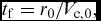 ${t_{\rm{f}}} = {{{r_0}}/ {{V_{{\rm{c,0}}}}}},$ respectively. Sampling time is taken to be T s = 0.05 s, because the laser coordinator gives information on the target location 20 times per second.
In order to start the Kalman filter, we need initial covariance matrix P0 for Ricatti equations calculation as the first filter tuning element. A particularly useful form of the homing loop model was given in Reference ZarchanRef. 12, where only diagonal elements are used:
 $$\begin{equation}
{{{\bf P}}_0} = \left[ {\begin{array}{@{}*{2}{c}@{}} {{{({\sigma _\lambda }r)}^2}}&0\\ 0&{{{(V\;HE)}^2}} \end{array}} \right]
\end{equation}$$
In the previous equation, the initial error in the estimate of position is simply the variance of measurement noise of our pseudo-measurement Equation (12), where the LOS angle, measured by the laser seeker, is corrupted with the assumed Gaussian noise of σλ = 1 mrad. The initial guess in the velocity error estimate is related to the missile velocity and the expected heading error (HE). The other filter tuning element is the process noise matrix Qk, where the process noise model is considered to be a target manoeuvre of constant amplitude with starting time uniformly distributed over the total time of flight. In Reference ZarchanRef. 12, it was mathematically shown that the equivalent shaping filter is white noise through an integrator, so the spectral density of this white noise process is given by:
 $$\begin{equation}
{\Phi _{\rm{s}}} = \frac{{w_0^2}}{{{t_{\rm{f}}}}}
\end{equation}$$
In the case of a slowly manoeuvring target, we still have the gravity in the vertical plane, where the gravity compensation is included as an equivalent target manoeuvre, so take:
 $$\begin{equation}
{w_0} = g\cos {\theta _0}
\end{equation}$$
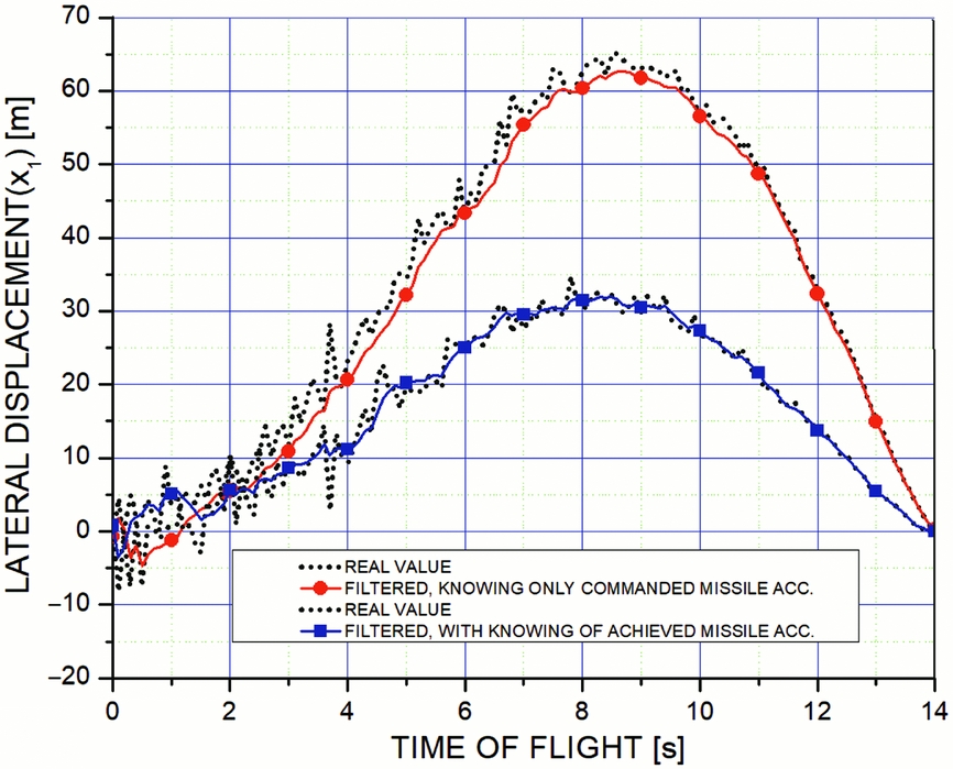
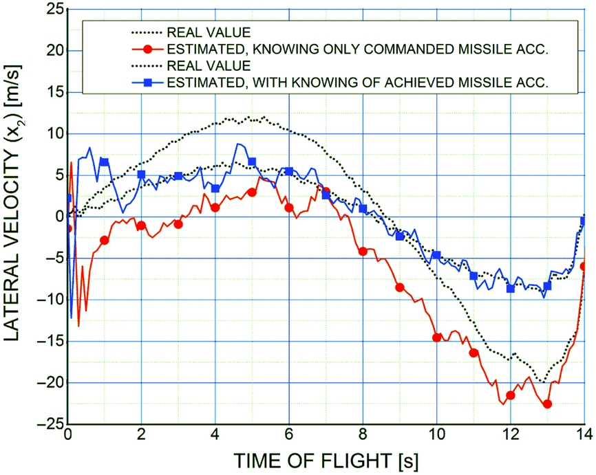
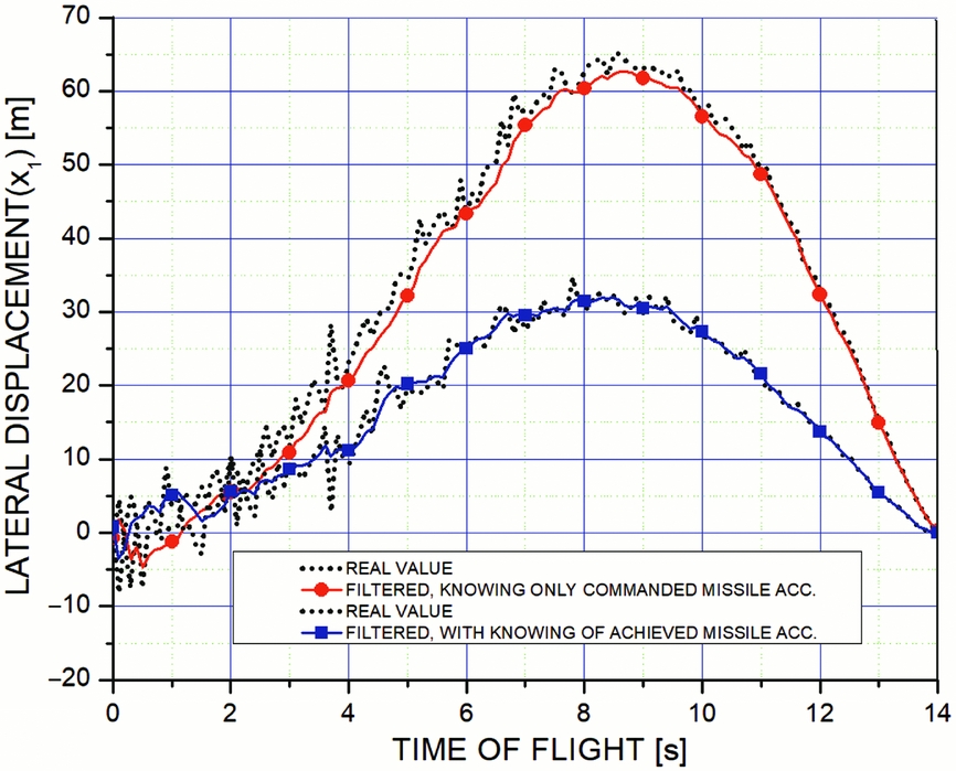
In Fig. 3, lateral displacements from the initial LOS are shown. In Fig. 4, lateral velocities, as the second state variable, for two different structures of the Kalman filter are presented.
Lateral displacement (real and filtered).
Lateral velocity (real and estimated).
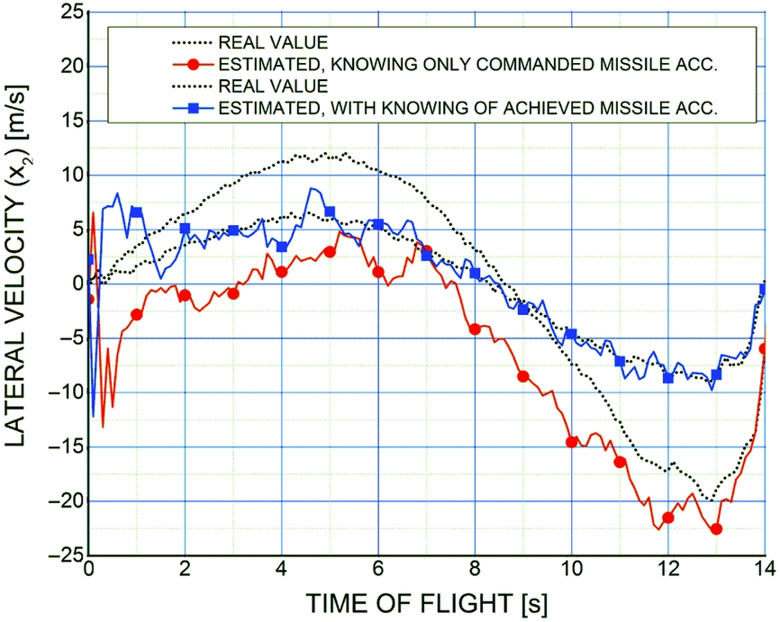
After LOS rate estimation using Kalman filter, it is used as an input to optimal guidance law in order to get the commanded lateral acceleration as output from the optimal guidance law, as shown in Fig. 2. When the lateral acceleration is obtained, two cases may take place. In the first case, the filter had only information about the command (requested lateral acceleration) where the switch on the block diagram is in position 2. In the second case, an accelerometer is introduced in order to measure the achieved lateral accelerations; the switch is in position 1. It is observed that the second case gives better results, because in such way, the system lags are eliminated in actuators and in the airframe using the Kalman filter since it filters both commanded and achieved lateral acceleration. The final result is achieved after two consecutive filtrations of lateral acceleration.
In the following analysis, the effect of different guidance laws on trajectory shape and commanded lateral acceleration is given. Optimal guidance, proportional navigation, and guidance with the aerodynamic sensor are considered.
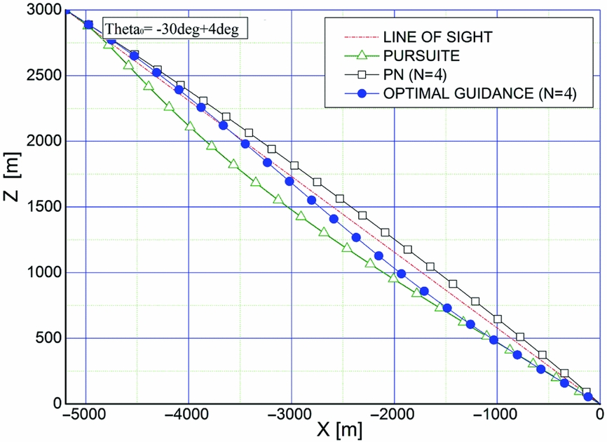
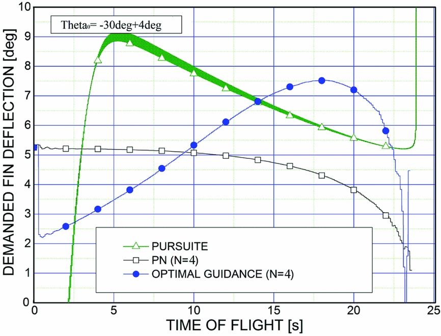
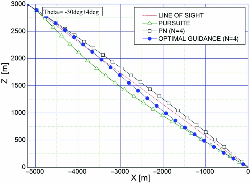
In the start point of the simulation, bomb–target distance is 6 km with LOS angle of θ0 = −30°, i.e. x 0 = −5196 m, z 0 = −3000 m, and the bomb is launched with heading error of HE = 4° above the initial LOS.
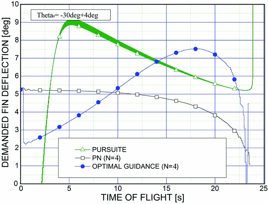
Gravity compensation in the vertical plane has been introduced as an equivalent target manoeuvre influencing the term w 0 in Equation (7). According to Fig. 5, the obtained results from the trajectory simulation show a good agreement with those expected since they achieve the target. It is also remarkable that both PN and optimal guidance methods don't have a big curved trajectory unlike the pursuit guidance method which gives the most curved trajectory. From Fig. 6, it is clearly shown that the pursuit guidance method requires the largest amount of energy during the guidance phase, especially at the beginning. During the pursuit method simulation, laser coordinator angle limitation has not been included because time flight limit is achieved while the target goes out of the field of view so that the guidance method cannot be used. Concerning the two remaining methods, PN guidance law and optimal guidance law, the common advantage is that they don't require a big amount of energy during the guidance phase. However, the PN guidance law requires a complicated and expensive mechanical construction (gimballed homing head and tracking system) which justifies the use of the optimal guidance law to achieve the target with low cost and efficient system.
Trajectories for different guidance laws.
Strap-down (non-gimballed) homing head.
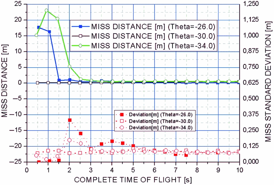
Statistical analysis of the optimal guidance method has been conducted by 50 runs of simulation execution for each total flight time in 0.5 s step increments, and miss distance has been considered in dependence on the total flight time. Analysed heading errors are − 4°, 0°, 4°, and the results of an analysis are shown in Fig. 7.
Terminal miss distance and deviation.
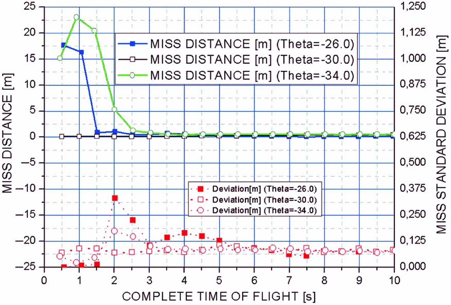
Figure 7 shows that minimal time of flight has to be 4 s in order to achieve terminal miss distance less than 1 m. The corresponding minimal bomb-to-target launching distance is 1 km, for missile velocity of 250 ms − 1.
5.0 CONCLUSION
In this paper, the optimal guidance law for a laser guided aerial bomb is successfully applied. Filtering the measured values and estimation of the missing state variables are done by a second-order Kalman filter. It is shown that the measuring of the achieved lateral acceleration and its use in the structure of the filter is necessary to improve performance.
Comparative analysis of different guidance laws is done along with their performance in a realistic pursuer–evader engagement study and the advantages of some of them and faults of the others are shown. The complete research is very relevant in the context of the state estimation and missile guidance in a practical environment.
Statistical analysis is performed in order to get terminal miss distance as a function of total flight time. Limits of the minimal time of flight for the given miss distance are determined. In this way, the usability of the laser guided bomb with simplified mechanical construction and applied optimal guidance law are shown.
In future work, time-to-go estimation should be considered without the perfect knowledge of relative range and its rate as assumed in this paper.