



1. Introduction
The instability and laminar–turbulent transition of supersonic and hypersonic boundary layers have been extensively investigated for several decades (Fedorov Reference Fedorov2011). Numerous reviews outlining the laminar–turbulent transition were given by Saric et al. (Reference Saric, Reshotko and Arnal1998), Fedorov (Reference Fedorov2011), Zhong & Wang (Reference Zhong and Wang2012) and Lee & Chen (Reference Lee and Chen2019). The boundary layer within the external or internal flows of high-speed vehicles may inevitably encounter shock waves emanating from geometric variation of the surface (Gaitonde Reference Gaitonde2015). The shock wave/boundary layer interaction (SWBLI) has the capability to significantly alter the transition process with enriched physics (Cao et al. Reference Cao, Hao and Guo2024). SWBLI-induced laminar–turbulent transition in hypersonic flows has received extensive attention due to its potential to cause enhanced unsteadiness and surface heating, and possibly engine intake unstart (Sandham et al. Reference Sandham, Schülein, Wagner, Willems and Steelant2014). DNS and experiments conducted on various canonical configurations for SWBLI (Benay et al. Reference Benay, Chanetz, Mangin, Vandomme and Perraud2006; Willems et al. Reference Willems, Gülhan and Steelant2015; Roghelia et al. Reference Roghelia, Olivier, Egorov and Chuvakhov2017; Currao et al. Reference Currao, Choudhury, Gai, Neely and Buttsworth2020; Fu et al. Reference Fu, Karp, Bose, Moin and Urzay2021) have confirmed that strong interactions can facilitate the generation of streamwise streaks and laminar–turbulent transitions near reattachment.
As shown by Huerre & Monkewitz (Reference Huerre and Monkewitz1990), SWBLI can be unstable either as an oscillator or a noise amplifier. Correspondingly, there exist two distinct origins of transition to turbulence in such hypersonic flows. The first type arises from self-excited global instability (Theofilis Reference Theofilis2011). The role of this absolute instability has been extensively examined, in part because when the strength of flow separation is sufficiently prominent, three-dimensionality can be identified in diverse canonical configurations. The benchmark instances of global instabilities that promote three-dimensionality include the compression ramp flow (Cao et al. Reference Cao, Hao, Klioutchnikov, Olivier, Heufer and Wen2021a , Reference Cao, Hao, Klioutchnikov, Olivier and Wenb ; Hao et al. Reference Hao, Cao, Wen and Olivier2021; Cao et al. Reference Cao, Hao, Klioutchnikov, Wen, Olivier and Heufer2022), the double-wedge flow (Gs et al. Reference Gs, Dwivedi, Candler and Nichols2018), the double-cone flow (Hao et al. Reference Hao, Fan, Cao and Wen2022), the hollow-cylinder–flare flow (Li & Hao Reference Li and Hao2023) and the shock impingement on a flat plate (Robinet Reference Robinet2007; Hildebrand et al. Reference Hildebrand, Dwivedi, Nichols, Jovanović and Candler2018; Fu et al. Reference Fu, Karp, Bose, Moin and Urzay2021). During the nonlinear saturation stage, such three-dimensionality is able to initiate the onset of transition. For instance, Fu et al. (Reference Fu, Karp, Bose, Moin and Urzay2021) performed high-fidelity simulations employing an impinging shock on a flat plate with sufficiently strong interactions. The laminar–turbulent transition commences via the breakdown of near-wall streaks shortly downstream of the impingement, without the necessity of any external disturbances. For a compression ramp configuration (Cao et al. Reference Cao, Hao, Klioutchnikov, Wen, Olivier and Heufer2022), the global instability induces the emergence of streamwise counter-rotating vortices and boundary layer streaks, whose breakdown can result in transition to turbulence downstream of reattachment. Such studies (Fu et al. Reference Fu, Karp, Bose, Moin and Urzay2021; Cao et al. Reference Cao, Hao, Klioutchnikov, Wen, Olivier and Heufer2022) provide evidence that absolute instability can lead to transition, which is an alternative route for the laminar–turbulent transition. Therefore, when designing wind tunnel tests or computational fluid dynamics simulations, it is imperative to consider the impact of the absolute instability so as to construct a comprehensive picture of the transition route.
Another potential pathway of laminar-turbulent transition in SWBLI is through the convective instability. Depending on the form and amplitude of external disturbances, there are several origins or explanations for transition over a compression ramp, such as the Mack second mode (Cao et al. Reference Cao, Hao and Guo2024), Görtler instability (Hao et al. Reference Hao, Cao, Guo and Wen2023; Cao et al. Reference Cao, Hao and Guo2024), baroclinic effect (Dwivedi et al. Reference Dwivedi, Sidharth, Nichols, Candler and Jovanović2019) and nonlinear interactions between oblique waves (Lugrin et al. Reference Lugrin, Beneddine, Leclercq, Garnier and Bur2021; Dwivedi et al. Reference Dwivedi, Sidharth and Jovanović2022). Balakumar et al. (Reference Balakumar, Zhao and Atkins2005) employed DNS and linear stability analysis (LSA) at Mach 5.4 to trace the evolution of fixed-frequency two-dimensional (2-D) perturbations over a compression ramp of ramp angle 5.5
 $^\circ$
. Their results justified that Mack second mode exhibits a neutral state in the separation bubble, yet undergoing an exponential amplification both upstream of separation and downstream of reattachment. Using the resolvent analysis and LSA, Guo et al. (Reference Guo, Hao and Wen2025b
) found that the Mack second mode is neutral due to discontinuous unstable regions in the bubble and that low-frequency shear layer modes are amplified due to multiple Görtler instabilities. Novikov et al. (Reference Novikov, Egorov and Fedorov2016) conducted DNS of three-dimensional (3-D) broad-spectrum wavepackets propagating in the configuration of Balakumar et al. (Reference Balakumar, Zhao and Atkins2005). The simulation reported the initiation of turbulent spots downstream of reattachment. Butler & Laurence (Reference Butler and Laurence2021) performed experiments on the evolution of Mack second mode within an incipiently separated compression ramp flow. They observed that corner interactions triggered a rapid breakdown immediately downstream of reattachment at high Reynolds numbers, resulting in a faster transition than for a straight cone. Furthermore, their spectral proper mode decomposition (SPOD) analysis demonstrated that the energy for components with hundreds of kilohertz was not amplified in the separation bubble, while that with tens of kilohertz was evidently augmented. For a compression ramp flow at Mach 8, Huang et al. (Reference Huang, Cao, Hao, Guo and Wen2025) confirmed via DNS that Mack second mode and low-frequency streaks as a manifestation of Görtler instability coexist within the boundary layer. The amplification of Mack second mode and sinuous/varicose streaks initiates the vortex roll-up process, resulting in the formation of hairpin vortices and the ultimate breakdown. For more complicated configurations, Benitez et al. (Reference Benitez, Borg, Paredes, Schneider and Jewell2023a
) conducted experiments on a cone-cylinder-flare model in quiet wind tunnels. They further provided evidence that the Mack second mode was neutral in the bubble and that the amplification of lower-frequency oblique waves was likely to be associated with the first mode (Paredes et al. Reference Paredes, Scholten, Choudhari, Li, Benitez and Jewell2022). They also showed that the nonlinear interaction between different frequency bands resulted in the emergence of turbulent spots downstream of reattachment (Benitez et al. Reference Benitez, Borg, Scholten, Paredes, McDaniel and Jewell2023b
). These findings strongly signified that in contrast to the transition process triggered by the absolute instability, the counterpart by the convective instability is more intricate. This is partly because the broadband components in the free stream may induce different instability modes through the receptivity, such as the first mode, Mack second mode, Görtler mode, etc. These modes may coexist in the flow field and trigger the breakdown jointly. Moreover, there exist modal interactions among them, thereby complicating the transitional process.
The significance of upstream disturbances has been growingly recognised owing to numerous experimental and computational efforts. Lugrin and Threadgill et al. (Lugrin et al. Reference Lugrin, Beneddine, Leclercq, Garnier and Bur2021; Lugrin et al. Reference Lugrin, Beneddine, Garnier and Bur2022a
; Threadgill et al. Reference Threadgill, Hader, Singh, Tsakagiannis, Fasel, Little, Lugrin, Bur, Chiapparino and Stemmer2025) observed that oblique modes play a prominent role and that their nonlinear modal interactions can potentially generate streamwise streaks. Benitez et al. (Reference Benitez, Borg, Paredes, Schneider and Jewell2023a
,
Reference Benitez, Borg, Scholten, Paredes, McDaniel and Jewellb
) and Caillaud et al. (Reference Caillaud2025) found that both Mack second mode and the shear-layer instability participate in the breakdown process at Mach 6 in a cone-cylinder-flare configuration. Cao et al. (Reference Cao, Hao and Guo2024) further confirmed that the onset of breakdown strongly relies on the amplitude of external disturbances in a globally stable flow condition with a ramp angle of 10
 $^\circ$
. Mack second mode and breakdown of reattachment streaks dominate the transition subject to relatively low-amplitude and high-amplitude upstream disturbances, respectively. With a large ramp angle, absolute and convective instabilities coexist. In such a scenario, it remains poorly understood which instability is more significant in a realistic transitional flow. The roles of the two categories of instabilities are also probably associated with the interplay between them.
This paper endeavours to decouple and elucidate the roles of absolute and convective instabilities in hypersonic boundary layer transition, intending to facilitate a comprehensive understanding of the transition mechanism of separated flows in relatively quiet and noisy wind tunnel experiments. To this end, a series of DNS cases are designed with or without external disturbances, where in turn, the disturbances are introduced with different levels of strength and at different time instants.
The remainder of this paper is organised as follows. Section 2 provides a detailed description of the numerical method. Details about the benchmark flows and physical interpretation of different instability regimes are given in § 3. The results of stability analysis are presented in § 4. In § 5, laminar–turbulent transition scenarios and comparative analysis results are introduced. Section 6 gives concluding remarks.
2. Methodology overview
2.1. Direct numerical simulation
The current hypersonic compression ramp flow is directly simulated employing a finite-difference-method code, which has a high-order resolution in both time and space, and the capability of robust shock wave capturing. This code has been extensively applied to studies of hypersonic compression ramp flows (Cao et al. Reference Cao, Klioutchnikov and Olivier2019; Cao et al. Reference Cao, Hao, Klioutchnikov, Olivier, Heufer and Wen2021a , Reference Cao, Hao, Klioutchnikov, Olivier and Wenb ; Cao et al. Reference Cao, Hao, Klioutchnikov, Wen, Olivier and Heufer2022; Cao et al. Reference Cao, Hao, Guo, Wen and Klioutchnikov2023; Cao et al. Reference Cao, Hao and Guo2024; Huang et al. Reference Huang, Cao, Hao, Guo and Wen2025). The 3-D compressible Navier–Stokes equations in the Cartesian coordinate system are written in the following conservation form:
 \begin{equation} \frac {\partial \boldsymbol{U}}{\partial t}+\frac {\partial \boldsymbol{F}}{\partial x}+\frac {\partial \boldsymbol{G}}{\partial y}+\frac {\partial \boldsymbol{H}}{\partial z}=\frac {\partial {{\boldsymbol{F}}^{v}}}{\partial x}+\frac {\partial {{\boldsymbol{G}}^{v}}}{\partial y}+\frac {\partial {{\boldsymbol{H}}^{v}}}{\partial z}, \end{equation}
where
 $\boldsymbol{F}$
,
 $\boldsymbol{G}$
and
 $\boldsymbol{H}$
are the vectors of inviscid fluxes, and
 $\boldsymbol{F}^{v}$
,
 $\boldsymbol{G}^{v}$
and
 $\boldsymbol{H}^{v}$
denote the vectors of viscous fluxes in the
 $x$
,
 $y$
and
 $z$
directions, respectively. Here,
 $\boldsymbol{U}={{(\rho ,\rho u,\rho v,\rho w,\rho e)}^{{T}}}$
represents the vector of conservative variables. Detailed expressions can be found from Anderson & Wendt (Reference Anderson and Wendt1995). The symbol
 $\rho$
refers to the density, and
 $u$
,
 $v$
and
 $w$
are the flow velocities along the
 $x$
,
 $y$
and
 $z$
directions, respectively. The variable
 $e$
is the total energy per unit mass and the superscript
 $\text{T}$
denotes matrix transpose. To close the equation system, the equation of state for perfect gases is used with the specific gas constant
 $R=287$
 $\text{J}\,(\text{kg}\boldsymbol{\, }\text{K})^{-1}$
. The Prandtl number
 $Pr$
and the specific heat ratio
 $\gamma$
are set to 0.72 and 1.4, respectively. Concurrently, Sutherland’s law is employed to calculate the dynamic viscosity.
Regarding the numerical method, time integration is performed through an explicit third-order total variation diminishing Runge–Kutta scheme (Gottlieb et al. Reference Gottlieb and Shu1998). The weighted essentially non-oscillatory (WENO) scheme of fifth order is employed to discretise the inviscid fluxes (Jiang et al. Reference Jiang and Shu1996). A sixth-order central-difference scheme is adopted to discretise the viscous fluxes. Details related to the numerical schemes can be retrieved from Hermes et al. (Reference Hermes, Klioutchnikov and Olivier2012), Cao (Reference Cao2021), Cao et al. (Reference Cao, Hao, Klioutchnikov, Olivier and Wen2021b ) and Huang et al. (Reference Huang, Cao, Hao, Guo and Wen2025).
As for the 2-D base flow, the number of grid points spanning the streamwise (
 $x$
) and normal (
 $y$
) directions is 4200 and 320, respectively. As shown in Appendix A, this resolution is adequate to achieve mesh convergence. For 3-D cases, figure 1 shows the schematic of the 3-D computational domain with coordinate system and boundary conditions. The initial 3-D flow field is constructed as a homogeneous extension of the 2-D base flow along the spanwise direction. There are 264 grid points uniformly distributed along the spanwise direction over a width of 12.6 mm, which corresponds to a total number of
 $4200\times 320\times 264\approx 355$
million. This mesh resolution yields non-dimensional wall units located near the outflow region (
 $x/L\approx 2.4$
):
 ${{x}^{+}}\approx 9.66$
,
 ${{y}^{+}}\approx 0.83$
and
 ${{z}^{+}}\approx 13.4$
. Near the exit, at least 160 grid points are located along the wall-normal direction in fully developed turbulent boundary layers. Such grid resolution closely resembles the DNS set-up used for hypersonic wall-bounded flows by Huang & Duan (Reference Huang and Duan2017). In terms of boundary conditions, incoming flow parameters are uniformly enforced at the inflow and upper boundaries. For the outflow boundary, the extrapolation condition is employed. For the no-slip wall, isothermal conditions are specified with a temperature of 293 K. For the 3-D case, the periodic boundary condition is employed on the spanwise boundaries. More details are provided by Huang et al. (Reference Huang, Cao, Hao, Guo and Wen2025).
Schematic of the 3-D computational domain with coordinate system and boundary conditions.

Figure 1. Long description
A diagram of a 3-D computational domain with labeled boundaries and coordinate system. The domain is a rectangular prism with dimensions labeled in terms of L. The incoming flow boundary is on the left side, the outflow boundary is on the right side, and the periodic boundary is on the front and back sides. The isothermal no-slip wall is on the top side. The coordinate system is labeled with x/L, y/L, and z/L axes. The incoming flow boundary is marked with arrows pointing into the domain, the outflow boundary is marked with arrows pointing out of the domain, and the periodic boundary is marked with arrows indicating the periodic nature of the boundary. The isothermal no-slip wall is marked with a green line.
2.2. Linear stability analysis
The current LSA addresses the problem of the convective instability initiated by small-amplitude disturbances in compressible boundary layers. The employed in-house code has been verified by calculating a series of benchmark cases (Guo et al. Reference Guo, Gao, Jiang and Lee2020; Guo et al. Reference Guo, Gao, Jiang and Lee2021; Guo et al. Reference Guo, Shi, Gao, Jiang, Lee and Wen2022a , Reference Guo, Shi, Gao, Jiang, Lee and Wenb ; Huang et al. Reference Huang, Cao, Hao, Guo and Wen2025). The small-amplitude disturbance takes the ansatz
 \begin{equation} {\boldsymbol{{\phi }^{\prime }}}(x,y,z,t)=\boldsymbol{\varphi } (y){\text{e}^{\text{i}(\alpha x+\beta z-\omega t)}}+c.c., \end{equation}
where
 $\boldsymbol{\varphi } ={{(\hat {\rho },\hat {u},\hat {v},\hat {w},\hat {T})}^{{T}}}$
is the eigenfunction, and
 $\beta$
and
 $\omega$
represent the spanwise wavenumber and the angular frequency, respectively. The
 $c.c.$
symbol denotes the corresponding complex conjugate. The complex streamwise wavenumber reads
 \begin{equation} \alpha ={{\alpha }_{r}}+\text{i}{{\alpha }_{i}}, \end{equation}
where
 ${\alpha }_{r}$
represents the streamwise wavenumber and
 $-{\alpha }_{i}$
denotes the spatial growth rate.
Under the parallel-flow assumption, the linearised Navier–Stokes (LNS) equations are transformed into an eigenvalue problem. Subsequently, it is solved through a Chebyshev pseudo-spectral method to obtain the global eigenvalue spectrum. An iterative compact fourth-order difference scheme is employed to improve the accuracy of the eigenvalue and eigenfunction (Malik et al. Reference Malik1990).
2.3. Global stability analysis
The GSA serves to examine whether the flow can be intrinsically unstable without the input of external disturbances. An in-house GSA solver is employed to quantify the temporal stability of a 2-D base flow in response to 3-D small-amplitude perturbations. The vector of conservative variables
 $\boldsymbol{U}$
is decomposed into a 2-D steady solution
 $\boldsymbol{U}_{2\text{-D}}$
and a 3-D small-amplitude perturbation
 $\boldsymbol{U}^{\prime }$
:
 \begin{equation} \boldsymbol{U}(x,y,z,t)={\boldsymbol{U}_{2\text{-D}}}(x,y)+{\boldsymbol{U}^{\prime }}(x,y,z,t), \end{equation}
where the prime denotes perturbed variables. The LNS equation reads
 \begin{equation} \frac {\partial {\boldsymbol{U}^{\prime }}}{\partial t}+\frac {\partial {\boldsymbol{F}^{\prime }}}{\partial x}+\frac {\partial {\boldsymbol{G}^{\prime }}}{\partial y}+\frac {\partial {\boldsymbol{H}^{\prime }}}{\partial z}=\frac {\partial {\boldsymbol{F}^{v}}^{\prime }}{\partial x}+\frac {\partial {\boldsymbol{G}^{v}}^{\prime }}{\partial y}+\frac {\partial {\boldsymbol{H}^{v}}^{\prime }}{\partial z}. \end{equation}
The equation can be rewritten as
 \begin{equation} \frac {\partial {\boldsymbol{U}^{\prime }}}{\partial t}=\boldsymbol{\mathcal{A}}{\boldsymbol{U}^{\prime }}, \end{equation}
where
 $\boldsymbol{\mathcal{A}}$
represents the LNS operator. The perturbations are assumed to be harmonic and are periodic in the spanwise direction (Cao et al. Reference Cao, Hao, Klioutchnikov, Olivier, Heufer and Wen2021a
; Hao et al. Reference Hao, Cao, Wen and Olivier2021; Cao et al. Reference Cao, Hao, Klioutchnikov, Wen, Olivier and Heufer2022; Cao et al. Reference Cao, Hao, Guo, Wen and Klioutchnikov2023; Cao et al. Reference Cao, Hao and Guo2024; Huang et al. Reference Huang, Cao, Hao, Guo and Wen2025). The perturbation
 $\boldsymbol{U}^{\prime }$
appears in the form
 \begin{equation} {\boldsymbol{U}^{\prime }}(x,y,z,t)=\boldsymbol{\hat {U}}(x,y)\exp \left [ \text{i}\frac {2\pi }{\lambda }z-\text{i}({{\omega }_{r}}+\text{i}{{\omega }_{i}})t \right ]\!, \end{equation}
where
 $\boldsymbol{\hat {U}}$
denotes the 2-D eigenfunction,
 $\lambda$
represents the spanwise wavelength,
 ${\omega }_{i}$
is the growth rate and the angular frequency is represented by
 ${\omega }_{r}$
. Here,
 ${{\omega }_{r}}=2\pi f$
, where
 $f$
is the frequency. By substituting (2.7) into (2.6) and discretising the resultant equation using the finite volume method, the eigenvalue problem can be obtained:
 \begin{equation} {\unicode{x1D63C}}(\lambda )\hat {\boldsymbol{U}}=-\text{i}({{\omega }_{r}}+\text{i}{{\omega }_{i}})\hat {\boldsymbol{U}}, \end{equation}
where
 ${\unicode{x1D63C}}(\lambda )$
represents the global Jacobian matrix. Through an implicit restarted Arnoldi method in ARPACK, the solution to the eigenvalue problem is obtained. A shift-invert method is adopted to evaluate the associated eigenvalue spectrum effectively (Hao et al. Reference Hao, Cao, Wen and Olivier2021).
Given the use of a lower-upper decomposition of the global matrix during the inversion step, the shift-invert method is computationally expensive. To minimise the computational cost, the mesh resolution of the base flow for stability analysis is reduced to
 $1750 \times 240$
, with the length of the flat plate and the ramp both being 50 mm. Grid independence has been confirmed by comparing with another set of grid solution
 $2240 \times 320$
. The grid independence verification is depicted in Appendix B.
2.4. Resolvent analysis
In the resolvent analysis, the response of the 2-D base flow to external small-amplitude forcings
 $\boldsymbol{f}^{\prime }$
with temporal and spanwise periodicity is investigated. The operator form for the corresponding LNS equation reads
 \begin{equation} \frac {\partial {\boldsymbol{U}^{\prime }}}{\partial t}=\boldsymbol{\mathcal{A}} {\boldsymbol{U}^{\prime }}+\boldsymbol{\mathcal{B}} {\boldsymbol{f}^{\prime }}. \end{equation}
In (2.9), the operator
 $\boldsymbol{\mathcal{B}}$
constrains the forcing to a localised location x/L = 0.2 that is consistent with subsequent 3-D DNS. The expression of
 $\boldsymbol{f}^{\prime }$
is given by
 \begin{equation} {\boldsymbol{f}^{\prime }}(x,y,z,t)=\hat {\kern-2.5pt\boldsymbol{f}}(x,y)\exp \left ( \text{i}\frac {2\pi }{\lambda }z-\text{i}{{\omega }_{r}}t \right )\!. \end{equation}
Note that as time progresses towards infinity, all initial perturbations imposed on the base flow decay to zero. The long-term solution to (2.10) has the same form as the forcing, which is given by the following equation:
 \begin{equation} {\boldsymbol{U}^{\prime }}(x,y,z,t)=\hat {\boldsymbol{U}}(x,y)\exp \left ( \text{i}\frac {2\pi }{\lambda }z-\text{i}{{\omega }_{r}}t \right )\!. \end{equation}
Substituting (2.10) and (2.11) into (2.9) and discretising the result in the same manner as in the GSA, yield
 \begin{equation} \hat {\boldsymbol{U}}={\unicode{x1D64D}} \boldsymbol{\mathcal{B}} \hat {\kern-2.5pt\boldsymbol{f}}, \end{equation}
 \begin{equation} {\unicode{x1D64D}}={{(-\text{i}{{\omega }_{r}}{\unicode{x1D644}}-{\unicode{x1D63C}})}^{-1}}, \end{equation}
where
 $\unicode{x1D64D}$
is the resolvent matrix and
 $\unicode{x1D644}$
represents the identity matrix.
The fundamental objective of the resolvent analysis is to determine the forcing and response pairs that optimise the energy amplification, which is defined by
 \begin{equation} {{\sigma }^{2}}(\lambda ,{{\omega }_{r}})=\underset {{\hat {\kern-2.5pt\boldsymbol{f}}}}{\mathop {\max }}\,\frac {{{\big \| {\hat {\boldsymbol{U}}} \big \|}_{E}}}{{{\big \| \boldsymbol{\mathcal{B}}\hat {\kern-2.5pt\boldsymbol{f}} \big \|}_{E}}}. \end{equation}
In (2.14),
 $\sigma$
represents the optimal gain and the Chu energy is utilized to obtain the energy norm:
 \begin{equation} {{\big \| {\hat {\boldsymbol{U}}} \big \|}_{E}}={{\hat {\boldsymbol{U}}}^{*}}{\unicode{x1D648}}\hat {\boldsymbol{U}}, \end{equation}
where
 $\unicode{x1D648}$
denotes the weight matrix (Bugeat et al. Reference Bugeat, Chassaing, Robinet and Sagaut2019) and
 ${\hat {\boldsymbol{U}}}^{*}$
is the complex conjugate of
 $\hat {\boldsymbol{U}}$
. According to Sipp & Marquet (Reference Sipp and Marquet2013), Bugeat et al. (Reference Bugeat, Chassaing, Robinet and Sagaut2019) and Dwivedi et al. (Reference Dwivedi, Sidharth, Nichols, Candler and Jovanović2019), the optimisation equation (2.14) can be transformed into an eigenvalue problem:
 \begin{equation} {{\boldsymbol{\mathcal{B}} }^{*}}{{{\unicode{x1D648}}}^{-1}}{{{\unicode{x1D64D}}}^{\,*}}{\unicode{x1D648}}\,{{{\unicode{x1D64D}}}}\,\boldsymbol{\mathcal{B}}\, \hat {\kern-2.5pt\boldsymbol{f}}={{\sigma }^{2}}\hat {\kern-2.5pt\boldsymbol{f}}, \end{equation}
which is resolved by using ARPACK for given
 $\beta$
(
 $\beta ={2\pi }/{\lambda }$
) and
 ${\omega }_{r}$
in the regular mode. SuperLU is employed to determine the inverses of
 $\unicode{x1D64D}$
and its conjugate transpose. The maximum eigenvalue represents the optimal gain square and the corresponding eigenfunction represents the optimal forcing. Using (2.12) and (2.13), the optimal response can be immediately obtained.
3. Benchmark flows and physical interpretation of instability regimes
3.1. Flow conditions
A compression ramp consisting of a flat plate with a sharp leading edge and a ramp with a deflection angle of 15
 $^\circ$
is investigated. We previously simulated such a transitional compression ramp flow with a small Reynolds number shown in table 1 (Huang et al. Reference Huang, Cao, Hao, Guo and Wen2025), in which the Reynolds number based on the flat plate length is
 ${\textit{Re}_{L}}$
=
 $3.9\times {10^5}$
. Due to the small Reynolds number, the flow is purely induced by convective instability. We refer to this low-Reynolds-number case as Case A to distinguish it from Case B in the current study. The flow condition of Case A was identical to the experiment of Chuvakhov & Radchenko (Reference Chuvakhov and Radchenko2020): free stream Mach number
 $\textit{Ma}_\infty =8$
, static temperature
 ${T_\infty }=53.3$
K,
 ${\textit{Re}_{L}}$
=
 $3.9\times {10^5}$
, static pressure
 ${P_\infty }=353$
Pa and wall temperature
 ${{T}_{w}}=293$
K, corresponding to a wall-to-total temperature ratio (
 ${{T}_{w}}/{{T}_{0}}$
) of 0.4. The DNS result has been comprehensively compared with the experimental one to demonstrate the reliability and high fidelity of our DNS.
Flow conditions of Case A in our previous work (Huang et al. Reference Huang, Cao, Hao, Guo and Wen2025).

Table 1. Long description
A table summarizing flow conditions for Case A. The table has one row and eight columns. Column headers are Case, Ma∞, ReL, T∞, P∞, Tw, Tw/T0, and Ramp angle. Row A: Case, 8; Ma∞, 3.9 x 10^5; ReL, 53.3 K; T∞, 353 Pa; P∞, 293 K; Tw, 0.4; Ramp angle, 15°.
The case currently under consideration, referred to as Case B in table 2, is an extension of the previous study. The detailed flow conditions of Case B are:
 $\textit{Ma}_\infty =8$
,
 ${T_\infty }=53.3$
K,
 ${\textit{Re}_{L}}$
=
 $9.2\times {10^5}$
,
 ${P_\infty }=832$
Pa and
 ${{T}_{w}}=293$
K. The flat-plate and ramp lengths adopted in Case B are
 $L=50$
mm and
 ${{L}_{r}}=75$
mm, respectively. Clearly, the Reynolds number is now increased, which serves to create an absolutely unstable state. The highly unstable nature of Case B with self-excited instabilities will be elaborated via GSA in § 4.1.
Flow conditions of all the present simulations.

Table 2. Long description
A table with one row and eight columns summarizing the flow conditions for Case B. The columns are labeled Case, Ma∞, ReL, T∞, P∞, Tw, Tw/T0, and Ramp angle. The row provides specific values for each condition: Case B, Ma∞ of 8, ReL of 9.2 x 10^5, T∞ of 53.3 K, P∞ of 832 Pa, Tw of 293 K, Tw/T0 of 0.4, and a Ramp angle of 15 degrees.
Before moving forward, it is beneficial to establish the conceptual relationship between the current high-Reynolds-number flow (Case B) and the low-Reynolds-number flow (Case A) that was previously investigated (Huang et al. Reference Huang, Cao, Hao, Guo and Wen2025). The flow is globally stable and functions as a pure noise amplifier in Case A, as the separation bubble is insufficiently robust to support self-excited global oscillations. Accordingly, the linear stability framework employed in that low-Reynolds-number case, which includes linear stability theory for Mack second modes as well as resolvent analysis for convective amplification, is directly applicable for describing the long-time response to external disturbances. In comparison, the separation bubble is completely unstable in Case B due to the increased Reynolds number, as demonstrated by the unstable stationary and oscillatory global modes identified by GSA in § 4.1. In this regime, the linearised dynamics of the clean base flow are intrinsically unstable.
The resolvent analysis framework, which is applied to the converged steady laminar base flow, is a carry-over from the Case A framework. This operator is well defined and can describe the early-time convective amplification of external white-noise before the absolute instability has grown to a non-negligible amplitude (Regime I in § 3.4). What does not persist is the assumption that the base flow will remain unaltered. In the long term, the absolute instability will saturate nonlinearly and fundamentally alter the flow. The decoupling strategy (see table 3) is fundamentally based on this conceptual distinction, which explains why resolvent analysis is exclusively employed for Cases B2/B4 (simulated within Regime I) and not as a predictive tool for the saturated coexistence regimes (B1/B3). The reader is referred to § 4.2 for a detailed discussion of the scope and limitations of resolvent analysis in the present globally unstable setting.
Case details for numerical simulations. The classification of Cases B2 and B4 is supported by the projection analysis presented below.

Table 3. Long description
A table comparing different cases of numerical simulations with various parameters. The table has six rows and six columns. Column headers are: Cases, 3-D DNS start time, 3-D DNS end time, The timing of introducing external disturbances, Disturbance amplitude, Contributed by which type of instability. Row 1: Cases, B; 3-D DNS start time, t U infinity / L = 0; 3-D DNS end time, t U infinity / L = 28.8; The timing of introducing external disturbances, No external disturbances; Disturbance amplitude, 0.0 percent; Contributed by which type of instability, Entirely from absolute instability. Row 2: Cases, B 1; 3-D DNS start time, t U infinity / L = 28.8; 3-D DNS end time, t U infinity / L = 34.8; The timing of introducing external disturbances, t U infinity / L = 28.8; Disturbance amplitude, 2.5 percent; Contributed by which type of instability, Absolute and convective instabilities coexist. Row 3: Cases, B 2; 3-D DNS start time, t U infinity / L = 0; 3-D DNS end time, t U infinity / L = 6.0; The timing of introducing external disturbances, t U infinity / L = 0; Disturbance amplitude, 2.5 percent; Contributed by which type of instability, Predominantly convective instability. Row 4: Cases, B 3; 3-D DNS start time, t U infinity / L = 28.8; 3-D DNS end time, t U infinity / L = 34.8; The timing of introducing external disturbances, t U infinity / L = 28.8; Disturbance amplitude, 6.0 percent; Contributed by which type of instability, Absolute and convective instabilities coexist. Row 5: Cases, B 4; 3-D DNS start time, t U infinity / L = 0; 3-D DNS end time, t U infinity / L = 6.0; The timing of introducing external disturbances, t U infinity / L = 0; Disturbance amplitude, 6.0 percent; Contributed by which type of instability, Predominantly convective instability.
3.2. Two-dimensional base flow
Figure 2 illustrates the Mach number distribution of the 2-D base flow as well as the enlarged view within the separation bubble, superimposed with streamlines. A large separation bubble is formed near the corner due to the adverse pressure gradient. The separation and reattachment points are located at
 $x/L\approx$
0.35 and 1.44, respectively. As shown in figure 2(
 $b$
), there is a strong secondary separation, with the primary separation bubble fragmenting into multiple secondary bubbles. The preliminary observation may imply a globally unstable state under the current condition. In §§ 4.1 and 4.2, stability analysis will be performed to examine the stability of the 2-D base flow within the separation bubble, as well as near and downstream of reattachment.
Visualisation of 2-D base flow: (
 $a$
) Mach number contour and (
 $b$
) enlarged view superimposed with streamlines within the separation bubble.

3.3. Three-dimensional benchmark flow
Before clarifying the roles of absolute and convective instabilities, it is useful to illustrate the specifics of the 3-D benchmark flow (i.e. Case B). For this case, the destabilisation mechanism is entirely dominated by absolute instability, as no external disturbances are introduced.
Figure 3 shows the DNS results of instantaneous wall Stanton number distributions of Case B at different time instants. Here, the Stanton number is defined by
 \begin{equation} St=\frac {{{q}_{w}}}{{{\rho }_{\infty }}{{U}_{\infty }}{{C}_{p}}({{T}_{aw}}-{{T}_{w}})}, \end{equation}
where
 ${q}_{w}$
denotes the heat flux,
 ${C}_{p}$
is the specific heat capacity and
 ${T}_{aw}$
is the adiabatic wall temperature for turbulent flows. As seen in figure 3(
 $a$
), at
 ${t{U}_{\infty }/L}= 3.2$
, St exhibits a clearly 2-D pattern. At this stage, the influence of absolute instability on the entire flow field is negligible, with no evidence of three-dimensionality (i.e. Regime I in figure 4
 $a$
). In figure 3(
 $b$
), weak three-dimensionality emerges near the reattachment line at
 ${t{U}_{\infty }/L}= 14.4$
, marking the approach to the end of the exponential stage (Regime II) in figure 4(
 $a$
). As time progresses, the streaks on the ramp become increasingly pronounced, reaching near full development in figure 3(
 $d$
) at
 ${t{U}_{\infty }/L}= 20.8$
(i.e. Regime III in figure 4
a). The exponential and nonlinear growth dynamics of the flow field will be analysed through the temporal growth of the spanwise velocity shortly downstream of the ramp within the separation bubble.
Instantaneous wall Stanton number of Case B at different time instants: (
 $a$
)
 ${t{U}_{\infty }/L}= 3.2$
; (
 $b$
)
 ${t{U}_{\infty }/L}= 14.4$
; (
 $c$
)
 ${t{U}_{\infty }/L}= 17.6$
; (
 $d$
)
 ${t{U}_{\infty }/L}= 20.8$
and (
 $e$
)
 ${t{U}_{\infty }/L}= 25.6$
. Separation and reattachment positions are highlighted by iso-lines of zero skin-friction coefficient (
 ${{C}_{f}}=0$
).

To quantify the growth of three-dimensionality, the temporal evolution of the quadratic mean of spanwise velocity at a streamwise position is evaluated by
 \begin{equation} {{A}_{w}}=\sqrt {\frac {1}{{{N}_{y}}{{N}_{z}}}\sum \limits _{j=1}^{{{N}_{y}}}{\sum \limits _{k=1}^{{{N}_{z}}}{(w/{{U}_{\infty }})_{j,k}^{2}}}}. \end{equation}
In (3.2),
 ${N}_{y}$
and
 ${N}_{z}$
represent the total number of grid points in the normal and spanwise directions, respectively. Within the separation bubble (at
 $x/L=1.07$
), the temporal evolution of
 ${A}_{w}/{A}_{s}$
is illustrated in figure 4(
 $a$
). Here,
 ${A}_{s}$
denotes the average value of
 $A_w$
in the nonlinear saturation stage of Case B. This parameter
 ${A}_{w}/{A}_{s}$
can effectively characterise to what degree the absolute instability affects the entire flow field during time marching. Figure 4(
 $a$
) demonstrates various instability regimes, which will be elaborated in § 3.4. In the range
 ${t{U}_{\infty }/L}= 0$
to 7.0, there exists a transient growth stage of
 ${A}_{w}/{A}_{s}$
. After that,
 ${A}_{w}/{A}_{s}$
begins to grow exponentially until
 ${t{U}_{\infty }/L}= 17.6$
and then reaches the nonlinear saturation stage. Figure 4(
 $b$
) shows the temporal evolution of
 ${\textit{St}}$
downstream of reattachment at
 $x/L=1.8$
and
 $z/L=0.126$
. Obviously,
 ${\textit{St}}$
is nearly constant until it reaches the nonlinear saturation stage at the dimensionless instant
 ${\textit{tU}_{\infty }}/L=17.6$
. The observation suggests that the evolution of
 ${\textit{St}}$
downstream of reattachment is closely coupled with the absolute instability, which is intrinsic to the separation bubble (Cao et al. Reference Cao, Hao, Klioutchnikov, Wen, Olivier and Heufer2022).
(
 $a$
) Temporal evolution of
 ${A}_{w}/{A}_{s}$
within the separation bubble (at
 $x/L=1.07$
) of Case B. The slope of the red and green dashed lines denotes the respective growth rate of Mode 1 and Mode 3 obtained from GSA under the most unstable spanwise wavelength (see figure 5
 $c$
). The grey dashed line represents
 ${t{U}_{\infty }/L}= 6.0$
. Pink dashed lines represent
 ${t{U}_{\infty }/L}= 7.0$
and
 ${t{U}_{\infty }/L}= 17.6$
. (
 $b$
) Temporal evolution of
 ${\textit{St}}$
downstream of reattachment at
 $x/L=1.8$
(
 $z/L=0.126$
).

3.4. Physical interpretation of instability regimes and disturbance injection strategies for the examined flows
In this subsection, the physical interpretation of instability regimes in Case B and perturbation injection strategies for the examined flows will be elaborated.
To decouple the absolute and convective instabilities, it is imperative to meticulously design the timing and amplitude when adding external disturbances in the Case B series. Cases B2 and B4 are designed to isolate the convective instability by introducing the external forcing at
 ${t{U}_{\infty }/L}= 0$
and terminating the simulation at
 ${t{U}_{\infty }/L}= 6.0$
. This timing ensures that the simulation is confined to the initial stage, during which the absolute instability has not yet developed to a noticeable level. Contrastingly, Cases B1 and B3 are initiated from the saturated state of Case B at
 ${t{U}_{\infty }/L}= 28.8$
, where the absolute instability has already fully developed. The flow state is established by external forcing that is introduced at this instant, resulting in the coexistence of absolute and convective instabilities. As illustrated in figure 4(
 $a$
), the degree of absolute instability can be quantitatively represented by the amplitude of
 ${A}_{w}/{A}_{s}$
. The degree of absolute instability increases as the amplitude of
 ${A}_{w}/{A}_{s}$
gets closer to unity. Nonlinear saturation is achieved when the amplitude reaches unity, which is the stage of fully developed absolute instability. In Regime I (from
 ${t{U}_{\infty }/L}= 0$
to
 ${t{U}_{\infty }/L}= 6.0$
), the amplitude of
 ${A}_{w}/{A}_{s}$
is exceedingly small, measured at less than
 $2 \times 10^{-5}$
. In Regime III (from
 ${t{U}_{\infty }/L}= 17.6$
to
 ${t{U}_{\infty }/L}= 28.8$
), i.e. the nonlinear saturation stage, the amplitude of
 ${A}_{w}/{A}_{s}$
is of the order of unity, approximately 50 000 times that of Regime I. Such a small level of
 ${A}_{w}/{A}_{s}$
in Regime I indicates that the contribution of absolute instability to the three-dimensionality is particularly weak (see figure 3
 $a$
). Therefore, Regime I is referred to as the weak absolute instability stage. Note that the regime separation primarily comes from the empirical comparison between saturated absolute instability cases (B1 and B3) and suppressed absolute instability cases (B2 and B4). The current
 ${A}_{w}/{A}_{s}$
serves as a supporting indicator. The flow parameters of Cases B1, B2, B3 and B4 are identical to those of Case B (see table 2). The differences among these five cases lie in whether external disturbances are applied or not and the injection timing of external disturbances, as shown in table 3.
For Case B, no external disturbance is introduced into the flow field during the DNS. Therefore, the destabilisation mechanism is entirely from the absolute instability, i.e. self-excited. For Cases B1, B2, B3 and B4, random forcing is introduced upstream of the separation point, taking the form of white noise
 $w_{j,k}^{\prime }/{{U}_{\infty }}={{\phi }_{n}}(2r-1)$
. Here,
 $w_{j,k}^{\prime }$
denotes the spanwise velocity perturbation imposed on all the grid nodes in the
 $y$
–
 $z$
plane at
 $x/L=0.2$
, and the indices
 $j$
and
 $k$
are along the normal and spanwise directions, respectively. Here,
 ${\phi }_{n}$
represents the amplitude of perturbations and
 $r$
denotes a pseudo-random number that varies from 0 to 1 (Cao et al. Reference Cao, Hao, Guo, Wen and Klioutchnikov2023; Huang et al. Reference Huang, Cao, Hao, Guo and Wen2025). For Cases B1 and B2, the amplitude of external disturbances
 ${{\phi }_{n}}=2.5\, \%$
. For Cases B3 and B4,
 ${{\phi }_{n}}=6.0\, \%$
. Conventional hypersonic wind tunnels generally exhibit free stream noise levels ranging from 1 % to 5 % (Bounitch et al. Reference Bounitch, Lewis and Lafferty2011; Casper et al. Reference Casper, Beresh and Schneider2014; Munoz et al. Reference Munoz, Wu, Radespiel, Semper, Cummings, Duan and Schilden2019; Bearden et al. Reference Bearden, Padilla, Taubert and Craig2022; Hoffman et al. Reference Hoffman, LaLonde, Andrade, Chen, Bilbo and Combs2023; Zhao et al. Reference Zhao, Ma, Chen, Zhang, Hao and Wen2024), e.g. AEDC Tunnel 9 at Mach 10 reports 4.94 % (Bounitch et al. Reference Bounitch, Lewis and Lafferty2011) and the HHK-6 tunnel shows up to 3.4 % (Munoz et al. Reference Munoz, Wu, Radespiel, Semper, Cummings, Duan and Schilden2019). The disturbance amplitude of 2.5 % in our DNS is evidently within this range and the disturbance amplitude of 6.0 % is close to the wind tunnel noise level of AEDC Tunnel 9 at Mach 10. The above-mentioned data confirm that the selected perturbation amplitudes of 2.5 % and 6 % in our DNS can physically reflect the noise levels in conventional wind tunnels. The amplitude of 2.5 % is indicative of a conventional wind tunnel at a moderate noise level, while a disturbance amplitude of 6.0 % is at a relatively high level. In short, the currently selected noise levels are sufficient to cover most tunnel conditions.
For Case B1, the external disturbance is introduced at the end of the simulation of Case B (i.e.
 ${\textit{tU}_{\infty }}/L=28.8$
). At that time, absolute instability has already evolved to a saturated state and excited strong unsteadiness, evidenced by figures 3(
 $e$
) and 4(a,b). This signifies that in the 3-D flow field where absolute instability has been fully developed, convective external disturbance is superimposed onto the flow field. In this case, the upstream disturbance begins to be at play. Within the simulation range of Case B1, i.e. from
 ${\textit{tU}_{\infty }}/L=28.8$
to
 ${\textit{tU}_{\infty }}/L=34.8$
, absolute and convective instabilities coexist. The external disturbance is in the form of white noise (spanwise velocity perturbations
 $w'/{{U}_{\infty }}$
, where
 ${U}_{\infty }$
is the streamwise velocity of the free stream) on the whole
 $y$
–
 $z$
plane and is placed upstream of the separation point and downstream of the leading-edge shock (specifically, at
 $x/L=0.2$
). In Case B1, the amplitude of the white noise is 2.5 %. Hence, the breakdown to turbulence in Case B1 is triggered by the conjunction of absolute and convective instabilities.
For Case B2, the simulated time range is from
 ${\textit{tU}_{\infty }}/L=0$
to
 ${\textit{tU}_{\infty }}/L=6$
, which corresponds to Regime I in figure 4(
 $a$
). The disturbance is introduced at the start of the simulation of Case B2, i.e.
 ${\textit{tU}_{\infty }}/L=0$
. In this simulated time interval, the disturbances due to absolute instabilities have not had time to grow to a non-negligible level (see Regime I in figure 4
 $a$
, the level of
 ${A}_{w}/{A}_{s}$
is less than one in 50 000 of the fully developed flow dominated by absolute instability). The minor value of the parameter
 ${A}_{w}/{A}_{s}$
indicates that the base flow is clean and must not be affected by the self-excited instability visibly. The only underlying contribution comes from the upstream disturbance. Therefore, the impact of the absolute instability is intended to be minimised and the convective instability is considered isolated from the absolute instability. In other words, the destabilisation mechanism for this case is predominantly convective. The other setup, including the disturbance, and its form and amplitude remain identical to those in Case B1.
Cases B3 and B4 possess the same computational setup as Cases B1 and B2, respectively, except that the amplitude of the external disturbance is increased to 6.0 %. They are designed to reveal the effect of the disturbance amplitude on the transition. The other setup is kept unchanged to conduct comparative research.
In addition to the qualitative characterisation based on
 $A_w/A_s$
, we further quantify the signature of absolute instability by projecting the DNS perturbation field onto the real part of the most unstable GSA mode (Mode 1), consistent with the real-valued nature of the DNS perturbation field. The projection is performed over the separation bubble region
 $\varOmega$
(
 $x/L \in [0.35, 1.44]$
) using the spanwise velocity component.
To obtain a dimensionless and case-independent measure of the absolute instability signature, we introduce a modal projection coefficient
 $\mathcal{P}$
, defined as the normalised inner product between the DNS perturbation field and the GSA mode:
 \begin{equation} \mathcal{P} = \frac {|\langle w'_{\textit{DNS}},\ \mathrm{Re}(\hat {w}_{\textit{GSA}}) \rangle |}{\|w'_{\textit{DNS}}\| \boldsymbol{\cdot }\|\mathrm{Re}(\hat {w}_{\textit{GSA}})\|}, \quad \langle f,g \rangle = \sum _{\varOmega } f \boldsymbol{\cdot }g,\quad \|f\| = \sqrt {\langle f,f \rangle }. \end{equation}
This coefficient is the direct analogue of the cosine of the angle between two vectors, generalised to functions defined over the spatial domain. This normalisation eliminates the dependence on the arbitrary scaling of the GSA eigenfunction, making
 $\mathcal{P}$
a robust metric for comparing the absolute instability signature across different cases.
The projection analysis was performed on the final time instant of each case. For the pure absolute instability case (Case B),
 $\mathcal{P} = 0.79$
. For the coexistence regimes, the values are
 $\mathcal{P} = 0.69$
(Case B1,
 $2.5$
% forcing) and
 $\mathcal{P} = 0.61$
(Case B3,
 $6.0$
% forcing). In contrast, for the convective-dominated regimes (Cases B2 and B4, both confined to Regime I), the coefficients drop to
 $\mathcal{P} = 0.07$
and
 $0.05$
, respectively. These results indicate a clear quantitative separation between the coexistence regimes (
 $\mathcal{P} \gt 0.6$
) and the convective-dominated regimes (
 $\mathcal{P} \lt 0.1$
), providing quantitative corroboration that the absolute instability is indeed negligible in Cases B2 and B4, while it remains strong whenever the flow is initialised from the saturated state of Case B. This analysis provides supporting evidence for the regime classification in table 3 and supports the conclusion that although the absolute instability does not significantly affect the transition onset location, it remains active in coexistence regimes and can therefore modulate the detailed transition features.
(
 $a$
) Growth rates of the most unstable stationary Mode 1 and (
 $b$
) the frequency of the most unstable modes as a function of the spanwise wavelength, provided by GSA. (
 $c$
) Eigenvalue spectrum at
 ${{\lambda }_{z}/L} = 0.084$
(
 ${\lambda }_{z}$
= 4.2 mm) corresponding to the largest growth rate in panel (a). The blue highlighted symbols in panels (a) and (b) denote
 ${{\lambda }_{z}/L} = 0.084$
and
 ${{\lambda }_{z}/L} = 0.04833$
(
 ${\lambda }_{z}$
= 2.42 mm, the switching wavelength), respectively. Stationary modes: Modes 1, 2 and 5. Oscillatory modes: Modes 3 and 4.

Figure 5. Long description
Panel A: A scatter plot shows the growth rates of the most unstable stationary Mode 1 as a function of the spanwise wavelength. The x-axis is labeled λz/L and ranges from 0 to 0.4. The y-axis is labeled ωiL/U∞ and ranges from −1.0 to 1.5. A vertical dashed line at approximately 0.1 on the x-axis and a blue highlighted symbol at the same x-value are visible. Panel B: A scatter plot shows the frequency of the most unstable modes as a function of the spanwise wavelength. The x-axis is labeled λz/L and ranges from 0 to 0.4. The y-axis is labeled fL/U∞ and ranges from −0.25 to 0.5. A vertical dashed line at approximately 0.1 on the x-axis and a blue highlighted symbol at the same x-value are visible. Panel C: A scatter plot shows the eigenvalue spectrum at a specific spanwise wavelength corresponding to the largest growth rate in Panel A. The x-axis is labeled fL/U∞ and ranges from −0.4 to 0.4. The y-axis is labeled ωiL/U∞ and ranges from −2 to 1. Modes 1, 2, and 5 are stationary, while Modes 3 and 4 are oscillatory.
4. Stability analysis
4.1. Global stability analysis
Figures 5(
 $a$
) and 5(
 $b$
) depict the non-dimensional growth rates and frequencies of the most unstable stationary mode (Mode 1) in figure 5(
 $c$
) as a function of the spanwise wavelength, respectively. As shown in figure 5(
 $a$
), the largest growth rate of Mode 1 occurs at
 ${{\lambda }_{z}/L}\approx 0.084$
(
 ${\lambda }_{z}\approx$
4.2 mm), denoted by the blue highlighted symbol. This growth rate is used to compare with the slope of the exponential growth stage of DNS in figure 4(
 $a$
). Figure 5(
 $b$
) shows the frequency of the most unstable mode against the spanwise wavelength. In figure 5(
 $b$
), the most unstable global modes are stationary when
 ${{\lambda }_{z}/L}\gt 0.04833$
, whereas unstable oscillatory modes are in the range
 ${{\lambda }_{z}/L} \approx 0.025{-} 0.04833$
. The value
 ${{\lambda }_{z}/L}= 0.04833$
is called the switching wavelength here and the global mode is stable below
 ${{\lambda }_{z}/L}\approx 0.025$
. The eigenvalue spectrum at the wavelength
 ${{\lambda }_{z}/L}=0.084$
is shown in figure 5(
 $c$
). In addition to Mode 1, two other stationary modes (Mode 2 and Mode 5) and two oscillating modes (Mode 3 and Mode 4) are identified. At the most unstable spanwise wavelength, the growth rate of Mode 1 is approximately 2.3 times that of Mode 3. As illustrated in figure 4(
 $a$
), the slope of the red and green dashed lines denotes the respective growth rate of Mode 1 and Mode 3 obtained from GSA under the most unstable spanwise wavelength. The slope of the red dashed line matches well with the evolution of
 ${A}_{w}/{A}_{s}$
in the exponential growth stage. It signifies that Mode 1 dominates the evolution of perturbations until the separation bubble reaches its nonlinear saturation stage. For Mode 3 and Mode 4, the corresponding Strouhal numbers are
 $fL/{{U}_{\infty }}\approx 0.25599$
(
 $f\approx$
6 kHz) and
 $fL/{{U}_{\infty }}\approx 0.43607$
(
 $f\approx$
10.2 kHz), respectively. Mode 3 possesses a slightly higher growth rate than Mode 4. The oscillation frequency of Mode 3 will then be compared with DNS later.
Iso-surfaces of
 $w/{{U}_{\infty }}= \pm 0.0014$
from DNS at
 ${\textit{tU}_{\infty }/L}=14.4$
of Case B. The numerical schlieren is superimposed at
 $z/L=0$
to demonstrate positions of separation and reattachment points.

(
 $a$
) Instantaneous distribution of the spanwise velocity
 $w/{{U}_{\infty }}$
obtained from DNS in the exponential growth stage (
 ${\textit{tU}_{\infty }/L}=14.4$
) in the
 $x$
–
 $y$
plane at
 $z/L=0.126$
of Case B. (
 $b$
) Real part of the spanwise velocity perturbation
 $\hat {w}/{{U}_{\infty }}$
for Mode 1 at
 ${{\lambda }_{z}/L}=0.084$
obtained from GSA. (
 $c$
) Enlarged view of
 $w/{{U}_{\infty }}$
in the
 $y$
–
 $z$
plane at
 $x/L=1.07$
at the same time instant with panel (
 $a$
).

Figure 6 displays the iso-surface of spanwise velocity
 $w/{{U}_{\infty }}= \pm 0.0014$
obtained from DNS at
 ${\textit{tU}_{\infty }/L}=14.4$
, which is in the exponential growth stage of Case B. As shown, the spanwise velocity obtained from DNS is primarily constrained within the separation bubble with an alternating positive–negative distribution pattern. As a comparison between GSA and DNS, figure 7 shows the instantaneous distribution of
 $w/{{U}_{\infty }}$
in the
 $x$
–
 $y$
plane (at
 $z/L=0.126$
) and
 $y$
–
 $z$
plane (at
 $x/L=1.07$
) obtained from DNS at
 ${\textit{tU}_{\infty }/L}=14.4$
of Case B, and the real part of the spanwise velocity perturbation
 $\hat {w}/{{U}_{\infty }}$
for Mode 1 at
 ${{\lambda }_{z}/L}=0.084$
obtained from GSA. As illustrated again, the spanwise velocity obtained from DNS and GSA exhibits a similar alternating positive–negative distribution pattern. An average spanwise wavelength
 ${\lambda }_{z}/L\approx$
0.084 (
 ${\lambda }_{z}\approx$
4.2 mm) is reported from DNS, which agrees well with the GSA. The good agreement implies that the exponential growth of the separation bubble is dominated by the GSA mode, provided that no external disturbance is imposed.
Estimated from figures 3(
 $d$
) and 3(
 $e$
), the mean spanwise wavelength is about 2.1 mm, which is about one half of the GSA result (4.2 mm). To clarify the discrepancy between DNS and GSA results, the quantified spatial spectra will be analysed later to reveal the space scales in the exponential growth and nonlinear saturation stages. Figure 8 presents the spanwise Fourier transforms of the spanwise velocity on the
 $x$
–
 $z$
plane at
 ${{y}_{n}}/L=0.005$
within the boundary layer. The contour is plotted versus the streamwise coordinate
 $x/L$
and the spanwise wavelength
 ${{\lambda }_{z}}/L$
in the exponential growth and nonlinear saturation stages. The ensemble average of the Fourier-transformed spanwise velocity with hundreds of snapshots is taken to minimise the randomness effect. In the exponential growth stage, the preferential spanwise wavelength spans from
 ${{\lambda }_{z}}/L\approx 0.08$
to
 ${{\lambda }_{z}}/L\approx 0.145$
, and the most amplified spanwise wavelength 0.084 obtained from GSA falls within this range. This confirms that DNS results clearly capture the spatial characteristics in the exponential growth stage. In figure 8(
 $b$
), two preferential spanwise wavelengths occur in the nonlinear saturation stage: one corresponds to the most amplified GSA mode, while the other pertains to the spanwise wavelength
 ${{\lambda }_{z}}/L\approx 0.042$
(
 ${{\lambda }_{z}}\approx$
2.1 mm). This new peak is the second harmonic mode of the most amplified GSA mode.
Spanwise Fourier transforms of the spanwise velocity on the
 $x$
–
 $z$
plane at
 ${{y}_{n}}/L=0.005$
in the (
 $a$
) exponential growth stage and (
 $b$
) nonlinear saturation stage. Ensemble average of the result is taken from
 ${t{U}_{\infty }/L}= 8.0$
to 16.0 in the exponential growth stage and from
 ${t{U}_{\infty }/L}= 20.8$
to 28.8 in the nonlinear saturation stage.
 ${y}_{n}$
denotes the wall-normal coordinate that starts from the wall.

From the perspective of mode-mode interactions in the Fourier space, the emergence of the second harmonic mode can be described by
 \begin{equation} (0,{{\beta }_{0}})\text{ }+\text{ }(0,{{\beta }_{0}})\to (0,2{{\beta }_{0}}), \end{equation}
where
 ${\beta }_{0}$
represents the fundamental spanwise wavenumber (i.e.
 ${{\beta }_{0}}={2\pi }/{{{\lambda }_{z0}}}$
,
 ${{{\lambda }_{z0}}}=$
4.2 mm). Mode
 $(0,{{\beta }_{0}})$
is the most amplified stationary GSA mode (Mode 1) and Mode
 $(0,2{{\beta }_{0}})$
is the generated second harmonic through nonlinear interactions. This signifies that during the switch from the linear growth stage to the nonlinear saturation stage, each streamwise streak bifurcates into two branches. Note that the small-wavelength range can also belong to the primary unstable oscillatory mode in figure 5(
 $b$
). Nonetheless, the wavelength of the oscillatory GSA mode is not constant and growth is dominated by the stationary mode in figure 4(
 $a$
). Therefore, the 2.1 mm component is the second harmonic of the stationary Mode 1.
Figure 9 presents the PSD results of the DNS spanwise velocity, temperature and pressure within the separation bubble and shortly downstream of reattachment. It is evident that the PSD results exhibit a broadband low-frequency feature. The dominant 6 kHz component of the GSA oscillatory mode (Mode 3) also falls well in the pronounced low-frequency band. Cao et al. (Reference Cao, Hao, Klioutchnikov, Olivier and Wen2021b
) have confirmed that such a low-frequency feature originates from the separation bubble. After examining the PSD results in the transitional region (
 $x/L=2.1$
), such a low-frequency feature still exists (not shown here). It is inferred that such a low-frequency feature can be seeded to propagate until the transitional region. In Appendix C, transitional images of Case B triggered by absolute instability are clearly identified, which resembles the results of Fu et al. (Reference Fu, Karp, Bose, Moin and Urzay2021) and Cao et al. (Reference Cao, Hao, Klioutchnikov, Wen, Olivier and Heufer2022) without introducing any external disturbances.
PSD results of (
 $a$
) spanwise velocity (
 $b$
) temperature and (
 $c$
) pressure within the separation bubble (
 $x/L=1.1$
), and shortly downstream of reattachment (
 $x/L=1.5$
) at
 $z/L=0.126$
and
 ${{y}_{n}}/L=0.005$
for Case B.

Figure 9. Long description
Panel A: A line graph shows the power spectral density (PSD) of spanwise velocity within the separation bubble. The x-axis represents frequency (f) in kilohertz (kHz) on a logarithmic scale, and the y-axis represents PSD on a logarithmic scale. Two lines are plotted: one for x/L = 1.1 (black) and another for x/L = 1.5 (red). The black line shows a steeper decline in PSD with increasing frequency compared to the red line. Panel B: A line graph displays the PSD of temperature within the separation bubble. The axes are the same as in Panel A. The black line (x/L = 1.1) shows a more pronounced drop in PSD with increasing frequency than the red line (x/L = 1.5). Panel C: A line graph illustrates the PSD of pressure within the separation bubble. The axes are identical to those in Panels A and B. The black line (x/L = 1.1) again shows a steeper decline in PSD with increasing frequency compared to the red line (x/L = 1.5).
4.2. Resolvent analysis
In the present study, the base flow used for resolvent analysis is a converged 2-D steady solution of the Navier–Stokes equations. The relation
 $\hat {\boldsymbol{U}}={\unicode{x1D64D}} \boldsymbol{\mathcal{B}} \hat {\kern-2.5pt\boldsymbol{f}}$
conveys information about the input–output linear mapping, irrespective of the global instability status. In this context, the resolvent operator
 $\unicode{x1D64D}$
manifests the linear dynamics about the clean base flow
 $\boldsymbol{\overline {U}}$
, where
 $\boldsymbol{\overline {U}}$
exactly satisfies the steady governing equations. The clean flow is the state at the very beginning when the absolute instability has no visible impact on the entire flow field. Thus, the eigen analysis of the resolvent operator constructed from this
 $\boldsymbol{\overline {U}}$
characterises how external white noise is amplified before the absolute instability increases to a certain amplitude and can then alter the base state. The resolvent analysis is strictly constrained to the discussion in a finite time interval, ensuring that the base flow remains valid. For instance, the resolvent analysis is only compared with DNS results in Cases B2 and B4, where the simulation time (
 ${\textit{tU}_{\infty }/L}=6.0$
) is earlier than the instant when the absolute instability begins to increase exponentially. In this stage, the normalised amplitude
 ${A}_{w}/{A}_{s}$
, characterising the baseline global instability, is less than
 $2 \times 10^{-5}$
. Under these conditions, the resolvent operator provides a reasonable model for the forced response, essentially capturing the convective-instability mechanism in the initial stage.
(
 $a$
) Contour of the optimal gain in the space of spanwise wavenumber and angular frequency. The gain is maximal when
 $\beta L\approx 260.8$
(marked with a pink circle), as the frequency
 ${{\omega }_{r}}L/{{U}_{\infty }}$
is approaching zero. An additional local maximum of the optimal gain can be identified at
 $\beta L=0$
(blue circle) when
 ${{\omega }_{r}}L/{{U}_{\infty }}\approx 135$
. (
 $b$
) Optimal gain as a function of the angular frequency at the most amplified spanwise wavenumber
 $\beta L=260.8$
.

Note that this approach has a limited application scope: resolvent analysis here is not employed to predict a long-term instability or the fully saturated nonlinear state. Rather, it functions as a supplementary tool to identify the most responsive convective modes to external forcing. The resolvent analysis establishes a baseline to understand the amplification mechanism before absolute instabilities have a notable impact on the entire flow field. It provides a mechanistic interpretation of the early transition stages. More importantly, resolvent analysis is not used in isolation. The spatial and frequency scales predicted by the resolvent analysis will be compared with DNS results of Cases B2/B4 with caution. The mutual verification between DNS and resolvent analysis shown in § 5.2 will further justify this issue.
2-D base flow solutions are utilized to conduct resolvent analysis that spans a wide range of spanwise wavelengths and angular frequencies. The spanwise wavenumber ranges from
 $\beta L=0$
to 600 and
 ${{\omega }_{r}}L/{{U}_{\infty }}$
from 0.1 (
 $f$
= 372 Hz) to 199.5 (
 $f$
= 742 kHz). It is worth noting that the forcing is located at
 $x/L=0.2$
, which is consistent with the 3-D DNS.
The resulting optimal gain is depicted in the
 $\beta$
–
 ${\omega }_{r}$
space in figure 10(
 $a$
). The gain is maximal when
 $\beta L\approx 260.8$
(
 ${{\lambda }_{z}}\approx$
1.2 mm) and the frequency
 ${{\omega }_{r}}L/{{U}_{\infty }}$
is approaching zero. Figure 10(
 $b$
) gives the optimal gain as a function of the angular frequency at the most amplified spanwise wavenumber
 $\beta L\approx 260.8$
. Clearly, the optimal gain almost remains constant at low frequencies and decays dramatically when
 ${{\omega }_{r}}L/{{U}_{\infty }}\gt 2$
. Such a low-frequency feature has also been observed in other studies of SWBLIs (Dwivedi et al. Reference Dwivedi, Sidharth, Nichols, Candler and Jovanović2019; Bugeat et al. Reference Bugeat, Robinet, Chassaing and Sagaut2022; Cao et al. Reference Cao, Hao, Guo, Wen and Klioutchnikov2023; Hao et al. Reference Hao, Cao, Guo and Wen2023). It has been confirmed that Görtler instability is the dominant amplification mechanism for streamwise streaks (Cao et al. Reference Cao, Hao, Guo, Wen and Klioutchnikov2023; Hao et al. Reference Hao, Cao, Guo and Wen2023). In figure 10(
 $a$
), an additional local maximum of the optimal gain can be identified at
 $\beta L=0$
when
 ${{\omega }_{r}}L/{{U}_{\infty }}\approx 135$
(
 $f\approx$
502 kHz), corresponding to the most amplified planar Mack second mode.
5. Laminar–turbulent transition and comparative analysis
5.1. Transition onset and breakdown to turbulence
Figure 11 illustrates the distribution of the spanwise- and time-averaged Stanton number in the streamwise direction. The theoretical correlations are plotted based on the following equation (Neumann et al. Reference Neumann and Hayes1986; Simeonides et al. Reference Simeonides1992):
 \begin{equation} {\textit{St}_{\textit {theory}}}=\frac {A}{s}{{\left[\frac {{{u}_{e}}{{P}_{e}}}{{{u}_{\infty }}{{P}_{\infty }}}\right]}^{1-n}}{{\left[\frac {{{T}_{\infty }}}{{{T}^{*}}}\right]}^{1-2n}}{{\left[\frac {{{C}^{*}}}{{{\textit{Re}}_{\infty ,x}}}\right]}^{n}}. \end{equation}
For a Prandtl number 0.72, the parameters (
 $A$
,
 $s$
,
 $n$
,
 $r$
) in (5.1) are (0.332,
 ${\textit{Pr}}^{2/3}$
, 0.5,
 ${\textit{Pr}}^{1/2}$
) and (0.0296, 1.0, 0.2,
 ${\textit{Pr}}^{1/3}$
) for laminar and turbulent flows, respectively. Here,
 ${T}^{*}$
is the reference temperature,
 ${C}^{*}$
denotes the Chapman–Rubesin linear viscosity factor (Chapman & Rubesin Reference Chapman and Rubesin1949) and
 ${u}_{e}$
,
 ${P}_{e}$
are local values at the edge of boundary layers. For more details, please refer to Roghelia et al. (Reference Roghelia, Olivier, Egorov and Chuvakhov2017).
Distributions of spanwise- and time-averaged wall Stanton number in the streamwise direction. Black and red solid lines represent laminar and turbulent theoretical correlations, respectively. Green squares, 2-D DNS results.

As shown in figure 11, downstream of reattachment, the 2-D DNS results coincide well with the laminar theoretical formula. For Case B, the flow does not develop to a fully developed turbulence flow (see also figure 33 in Appendix C), which yields deviations from the turbulent correlation. From Case B1 to Case B4, near the outflow boundary, the
 ${\textit{St}}$
numbers obtained from DNS collapse well onto the turbulent correlation, which indicates a fully developed turbulent state.
The elevated Stanton number observed in Cases B1 and B2 is a classic heat flux overshoot phenomenon, well documented in SWBLI in the transitional state. The overshoot occurs when the flow undergoes transition, but has not yet reached a fully developed turbulent state within the computational or experimental domain. This overshoot phenomenon has been extensively reported in both experimental (Benay et al. Reference Benay, Chanetz, Mangin, Vandomme and Perraud2006; Bur & Chanetz Reference Bur and Chanetz2009; Knight & Mortazavi Reference Knight and Mortazavi2018; Currao et al. Reference Currao, Choudhury, Gai, Neely and Buttsworth2020) and DNS studies (Cao et al. Reference Cao, Hao and Guo2024; Huang et al. Reference Huang, Cao, Hao, Guo and Wen2025) of hypersonic SWBLI flows. Specifically, Currao et al. (Reference Currao, Choudhury, Gai, Neely and Buttsworth2020) observed overshoots of approximately 15 % in hypersonic transitional SWBLI, while Lugrin et al. (Reference Lugrin, Nicolas, Severac, Tobeli, Beneddine, Garnier, Esquieu and Bur2022b ) reported overshoots up to 25 %. The causes of heat-flux overshoot are closely linked to the Görtler instability pertaining to the streamline curvature and the rapid transition at reattachment (Benay et al. Reference Benay, Chanetz, Mangin, Vandomme and Perraud2006; Currao et al. Reference Currao, Choudhury, Gai, Neely and Buttsworth2020).
The observed discrepancy in the
 ${\textit{St}}$
distribution is a result of the distinction in the disturbance amplitude and its subsequent impact on the transition physics. Cases B1 and B2 represent moderate disturbance levels (2.5 %), while Cases B3 and B4 correspond to large disturbance levels (6.0 %). This amplitude disparity fundamentally alters the transition dynamics. For large disturbance amplitudes, i.e. Cases B3 and B4, the strong convective disturbance accelerates the breakdown process, leading to rapid transition completion (see figures 15 and 16). Consequently, the spanwise- and time-averaged
 ${\textit{St}}$
profiles collapse onto the turbulent theoretical correlation just shortly downstream of reattachment. Under the moderate disturbance levels, i.e. Cases B1 and B2, the weak external disturbance triggers a slower and more gradual transition. The transition requires a longer distance to reach its fully turbulent state compared with the noisy cases. This developing state is characterised by elevated heat flux known as the overshoot phenomenon. This disturbance-amplitude dependent behaviour is physically consistent, since a large noise level case injects more energy into the instability modes, accelerates the nonlinear breakdown and shortens the transitional-region length. This interpretation is consistent with the findings of Benay et al. (Reference Benay, Chanetz, Mangin, Vandomme and Perraud2006) and Bur & Chanetz (Reference Bur and Chanetz2009), who showed that the heat flux overshoot can be mitigated by triggering an earlier transition to a fully turbulent SWBLI.
(
 $a$
) The r.m.s. distribution of the Stanton number fluctuation
 ${\textit{St}}{{'}_{\textit {rms}}}$
along the streamwise direction. The black dash dotted line denotes the threshold criterion
 ${\textit{St}}{{'}_{\textit {rms}}}=4\times {{10}^{-3}}$
. (
 $b$
) Transition onset locations based on different thresholds of
 ${\textit{St}}{{'}_{\textit {rms}}}$
for Cases B1–B4.

Figure 12. Long description
Panel A: A line graph shows the root mean square (r.m.s.) distribution of the Stanton number fluctuation along the streamwise direction. The x-axis is labeled x/L and the y-axis is labeled St_rms. The graph includes data for five cases: Case B, Case B1, Case B2, Case B3, and Case B4, each represented by different symbols and colors. A black dash-dotted line denotes the threshold criterion. Panel B: Another line graph displays transition onset locations based on different thresholds of St_rms for Cases B1 to B4. The x-axis is labeled Threshold and the y-axis is labeled Transition onset location. Each case is represented by different symbols and colors.
To reveal the impact of absolute and convective instabilities, the transition onset and end locations are imperative to be identified. Figure 12(
 $a$
) shows the root mean squared (r.m.s.) distribution of the Stanton number fluctuation
 ${\textit{St}}{{'}_{\textit {rms}}}$
averaged in the spanwise direction along the streamwise direction for all the five cases. The definition of
 ${\textit{St}}{{'}_{\textit {rms}}}$
is given by
 \begin{equation} \textit{St}{{'}_{\textit {rms}}}=\sqrt {\overline {{\textit{St}}^{\prime 2}}}, \end{equation}
where the long overline ‘—’ represents the arithmetic mean. Meanwhile,
 ${\textit{St}}'=St-{{\left \langle St \right \rangle }_{t}}$
, where
 ${\left \langle St \right \rangle }_{t}$
is the time-averaged value. As shown in figure 12(
 $a$
), the peak value of
 ${\textit{St}}{{'}_{\textit {rms}}}$
of Case B remains below
 $1.5\times {{10}^{-3}}$
. This value is considerably lower than the values of Cases B1–B4, implying that the transitional process of Case B is not as quick as the others. Consequently, the transition onset criterion proposed based on Cases B1–B4, which relies on a fixed threshold, was not applied to Case B. As a special case, the transition onset of Case B is determined based on the streamwise position where the spanwise- and time-averaged
 ${\textit{St}}$
number begins to exhibit a secondary increase. In the study of transitions induced by pure absolute instability by Cao et al. (Reference Cao, Hao, Klioutchnikov, Wen, Olivier and Heufer2022), they adopted the same criteria to determine the transition onset location. With the presence of convective instabilities, the transition is accelerated for Cases B1–B4 and there is no secondary increase in
 ${\textit{St}}$
. The different criteria indicate that the transition onset locations of Case B cannot be directly compared with the others. Nonetheless, it is clear that Case B transitions slower according to the mean
 ${\textit{St}}$
curves.
As shown in figure 12(
 $b$
), the selection of the threshold does not affect the relative magnitude of transition onset locations for different cases. The central conclusion is robust with respect to the choice, since a varied threshold within a reasonable range yields the same conclusion regarding the relative magnitude of transition onset locations. In this paper, the transition onset for Cases B1–B4 takes the streamwise position at which
 ${\textit{St}}{{'}_{\textit {rms}}}$
reaches a threshold
 ${\textit{St}}{{'}_{\textit {rms}}}\approx 4\times {{10}^{-3}}$
, which is nearly the peak value. This maximum-amplitude location for instability waves is usually in the vicinity of the breakdown point for the 3-D hypersonic transitional boundary layer (Guo et al. Reference Guo, Hao and Wen2023). Thus, the threshold value of
 $4\times {{10}^{-3}}$
serves as a representative criterion. The instantaneous visualisation of vortex structures of different cases is depicted in figures 13–16 and 33 to reveal the transitional and breakdown events of the flow field. For the moderate noise level cases (Cases B1 and B2), coherent vortices emerge near the reattachment line, followed by the formation of hairpin-like vortex packets that undergo gradual breakdown further downstream. For the large noise level cases (Cases B3 and B4), the vortex structures are more vigorous: streamwise vortices appear immediately downstream of reattachment and rapidly disintegrate into small-scale coherent structures. This amplitude-dependent behaviour confirms that a stronger convective forcing accelerates the nonlinear breakdown process, while the presence of absolute instability provides a secondary modulation to the overall breakdown scenarios.
Instantaneous visualisation of vortex structures of Case B1. The
 $Q$
-criterion coloured by
 $u/{{U}_{\infty }}$
is utilized to visualise the transitional and fully developed turbulent flow. The Stanton number contour is shown superimposed with isolines of zero skin friction coefficient. Numerical schlieren at
 $z/L=0$
is additionally added to highlight the separation and reattachment points. The upper left panel represents the zoomed-in view of the shock–shear layer patterns and coherent structures near the transitional boundary layer.

Based on the above-mentioned criterion, the transition onset locations are listed in table 4. For Case B, the onset of transition is at
 $x/L\approx 2.10$
and Appendix C provides a comprehensive overview of its transitional scenario. For Cases B1 and B2 where the external disturbance amplitude is 2.5 %, the transition onset locations are approximately
 $x/L\approx 1.68$
and
 $x/L\approx 1.77$
, respectively. This signifies that when absolute and convective instabilities coexist (Case B1), the position of transition onset is
 $\Delta x/L\approx 0.1$
earlier than where only convective instability is evident (Case B2). This minor advance indicates that the absolute instability does not affect the transition onset remarkably. As shown in figures 12 and 15–16, the locations of transition onset of Cases B3 and B4 are both
 $x/L\approx 1.55$
, given that the amplitude of external disturbances is increased to 6 %. In such situations, the role of the absolute instability is even weaker than that of the convective instability, thereby showing no visible difference in the transition onset. In other words, Cases B3 and B4 are dominated by the convective-type instability. By comparing Cases B1 and B3 (or B2 and B4), one finds that as the strength of the external disturbance increases, the transition onset position is moved forward more evidently than by the effect of the absolute instability.
Transition onset locations of the five cases.

Table 4. Long description
A table with two columns and five rows. The first column is labeled ‘Cases’ and the second column is labeled ‘Transition onset locations’. The rows are as follows: Row 1: Case B, x / L ≈ 2.10; Row 2: Case B1, x / L ≈ 1.68; Row 3: Case B2, x / L ≈ 1.77; Row 4: Case B3, x / L ≈ 1.55; Row 5: Case B4, x / L ≈ 1.55.
Instantaneous visualisation of vortex structures of Case B2. The
 $Q$
-criterion coloured by
 $u/{{U}_{\infty }}$
is utilized to visualise the transitional and fully developed turbulent flow. The Stanton number contour is shown superimposed with isolines of zero skin friction coefficient. Numerical schlieren at
 $z/L=0$
is additionally added to highlight the separation and reattachment points. The upper left panel represents the zoomed-in view of the shock–shear layer patterns and coherent structures near the transitional boundary layer.

Figure 14. Long description
Panel A: A heat map shows the Stanton number contour with isolines of zero skin friction coefficient. The x-axis represents the normalized streamwise distance (x/L) ranging from 0 to 2.50, and the y-axis represents the normalized spanwise distance (z/L) ranging from 0 to 1.50. The color scale indicates the Stanton number, with lighter colors representing higher values and darker colors representing lower values. Panel B: A heat map displays the numerical schlieren at a specific value, highlighting separation and reattachment points. The x-axis represents the normalized streamwise distance (x/L) ranging from 0 to 2.50, and the y-axis represents the normalized spanwise distance (z/L) ranging from 0 to 1.50. The color scale indicates the intensity of the numerical schlieren, with a gradient from blue to red. The upper left panel provides a zoomed-in view of the shock-shear layer patterns and coherent structures near the transitional boundary layer, with the -criterion colored by is.
Instantaneous visualisation of vortex structures of Case B3. The
 $Q$
-criterion coloured by
 $u/{{U}_{\infty }}$
is utilized to visualise the transitional and fully developed turbulent flow. The Stanton number contour is shown superimposed with isolines of zero skin friction coefficient. Numerical schlieren at
 $z/L=0$
is additionally added to highlight the separation and reattachment points. The upper left panel represents the zoomed-in view of the shock–shear layer patterns and coherent structures near the transitional boundary layer.

Instantaneous visualisation of vortex structures of Case B4. The
 $Q$
-criterion coloured by
 $u/{{U}_{\infty }}$
is utilized to visualise the transitional and fully developed turbulent flow. The Stanton number contour is shown superimposed with isolines of zero skin friction coefficient. Numerical schlieren at
 $z/L=0$
is additionally added to highlight the separation and reattachment points. The upper left panel represents the zoomed-in view of the shock–shear layer patterns and coherent structures near the transitional boundary layer.

Figure 16. Long description
Panel A: A heat map showing the Stanton number contour with isolines of zero skin friction coefficient. The color scale ranges from low to high values, indicating different levels of heat transfer. The numerical schlieren highlights separation and reattachment points. Panel B: A zoomed-in view of the shock-shear layer patterns and coherent structures near the transitional boundary layer. The -criterion colored by is used to visualize transitional and fully developed turbulent flow.
Apart from the differences in the transition onset location, the breakdown scenarios of Cases B1 to B4 are visibly similar. In proximity and downstream of reattachment lines, streamwise vortices appear, followed by the roll-up and lift of hairpin-like vortex structures. Taking Case B2 as an example, mesh sensitivity study of 3-D DNS is conducted in Appendix D, and one can observe a good agreement on the boundary layer profiles between DNS and theoretical predictions in Appendix E regarding the law of the wall and the mean temperature-velocity relation. As a result, a fully developed turbulent state is reached for most cases.
5.2. Spectral characteristics of transition scenarios
To further reveal the roles of absolute and convective instabilities, spatial and temporal spectral analysis is performed in this subsection. The analysis is categorised into two subsections. The first subsection (§ 5.2.1) analyses the fully evolved 3-D state, encompassing Cases B, B1 and B3, where the absolute instability either evolves purely from the outset (Case B) or has already been modulated by external white noise forcings after saturation (Cases B1 and B3). The second subsection (§ 5.2.2) examines the early-stage 2-D base state, encompassing Cases B2 and B4, where the absolute instability is suppressed by early termination and the flow is predominantly convective.
5.2.1. Role of convective instabilities on fully evolved 3-D base state: Cases B, B1 and B3
The long-duration evolved 3-D base state cases are first examined, which comprises the baseline absolutely unstable case (Case B) and the coexistence regimes at two disturbance amplitudes (Case B1, 2.5 % and Case B3, 6 %).
Common logarithm of modulus of spanwise Fourier transforms of
 ${\textit{St}}$
number on the wall (
 $x$
–
 $z$
plane) versus the streamwise coordinate
 $x/L$
for (
 $a$
) Case B1 (coexistence, 2.5 %) and (
 $b$
) Case B3 (coexistence, 6 %). The ensemble average is taken using several hundreds of snapshots. The key spanwise wavelengths are
 ${{\lambda }_{z}/L}\approx 0.084$
(
 ${{\lambda }_{z}}\approx 4.2$
mm, GSA fundamental) and
 ${{\lambda }_{z}/L}\approx 0.042$
(
 ${{\lambda }_{z}}\approx 2.1$
mm, GSA second harmonic).

Amplitude of spanwise Fourier transforms of
 ${\textit{St}}$
number on the wall (
 $x$
–
 $z$
plane) versus the spanwise wavelength
 ${\lambda }_{z}$
extracted at
 $x/L=1.5$
in figure 17 for (
 $a$
) Case B1 (coexistence, 2.5 %) and (
 $b$
) Case B3 (coexistence, 6 %).

Figure 17 depicts the common logarithm of modulus of spanwise Fourier transforms of
 ${\textit{St}}$
for Cases B1 and B3. The data are retrieved on the wall (
 $x$
–
 $z$
plane) versus the streamwise coordinate
 $x/L$
. Figure 18 shows the amplitude versus the spanwise wavelength
 ${\lambda }_{z}$
extracted at
 $x/L=1.5$
in figure 17 for Cases B1 and B3. For Case B1 in which absolute and convective instabilities coexist, the GSA mode wavelength
 ${{\lambda }_{z}}\approx 4.2$
mm becomes weaker, while
 ${{\lambda }_{z}}\approx 2.1$
mm of the second harmonic tends to be more pronounced. The 2.1 mm component arises from nonlinear mode-mode interactions (see (4.1)), where the fundamental GSA mode (
 ${{\lambda }_{z}}\approx 4.2$
mm) generates its second harmonic as the flow transitions from the linear growth stage to nonlinear saturation stage (Cao et al. Reference Cao, Hao, Klioutchnikov, Wen, Olivier and Heufer2022). Notably, by comparing figures 8, 17(
 $a$
) and 18(
 $a$
), the introduction of external noise serves to add broadband components to the wavenumber spectrum. Nonetheless, the signature of the absolute instability is not wiped by the external forcing in Case B1. As a result, the impact of the absolute instability remains in the transition process, albeit the transition onset location is not affected remarkably.
For Case B3, where the external forcing is added after absolute instability saturates, the GSA mode wavelengths 4.2 and 2.1 mm are less clear owing to a larger-amplitude forcing. The side band is filled by external noise to a larger extent. Additionally, we note that the resolvent optimal gain peak at
 ${{\lambda }_{z}}\approx 1.2$
mm appears in the purely convective regimes (Cases B2 and B4, see figures 21 and 22), not in Case B3.
Figures 19 and 20 characterise the spanwise-averaged modulus of the temporal Fourier transforms of the observed signals for Cases B, B1 and B3. The signals include the Stanton number in figure 19 and wall pressure in figure 20. In figure 20, dashed and solid lines represent the oscillatory GSA mode frequency
 $f\approx 6$
kHz and the frequency of the most unstable Mack second mode, respectively. The second-mode frequency is predicted by LSA.
Common logarithm of spanwise-averaged modulus of temporal Fourier transforms of
 ${\textit{St}}$
number on the wall (
 $x$
–
 $z$
plane) versus the streamwise coordinate
 $x/L$
for (
 $a$
) Case B (pure absolute instability), (
 $b$
) Case B1 (coexistence, 2.5 %) and (
 $c$
) Case B3 (coexistence, 6.0 %). The left vertical axis denotes the physical frequency, and the right vertical axis represents the dimensionless frequency, where
 ${{\omega }_{r}}=2\pi f$
.

Common logarithm of spanwise-averaged modulus of temporal Fourier transforms of the wall pressure on the
 $x$
–
 $z$
plane versus the streamwise coordinate
 $x/L$
for (
 $a$
) Case B (pure absolute instability), (
 $b$
) Case B1 (coexistence, 2.5 %) and (
 $c$
) Case B3 (coexistence, 6.0 %). Dashed and solid lines represent
 $f\approx 6$
kHz and the frequency of the most unstable planar Mack second mode, respectively. The left vertical axis denotes the physical frequency, and the right vertical axis represents the dimensionless frequency, where
 ${{\omega }_{r}}=2\pi f$
.

Figure 20. Long description
Panel A: A heatmap shows the common logarithm of spanwise-averaged modulus of temporal Fourier transforms of the wall pressure on the plane versus the streamwise coordinate for Case B (pure absolute instability). The x-axis is labeled x/L, and the y-axis is labeled f(kHz). The color bar indicates values ranging from −2.5 to −1.0. A dashed line represents a specific frequency. Panel B: A heatmap shows the same data for Case B1 (coexistence, 2.5 %). The x-axis is labeled x/L, and the y-axis is labeled f(kHz). A black line indicates a trend. Panel C: A heatmap shows the same data for Case B3 (coexistence, 6.0 %). The x-axis is labeled x/L, and the y-axis is labeled f(kHz). A black line indicates a trend.
For Case B, as shown in figures 19(
 $a$
) and 20(
 $a$
), the low-frequency signature below the frequency 6 kHz can propagate downstream into the transitional region (
 $x/L\gt 2.1$
). Ahead of the transition onset, no obvious high-frequency components are identified. This observation confirms that the transition of Case B is triggered by the low-frequency feature intrinsic to the separation bubble.
For Case B1, as shown in figure 19(
 $b$
), in addition to low-frequency components, the band with hundreds of kilohertz emerges. In figure 20(
 $b$
), the most unstable second mode frequency by LSA is consistent with DNS in the pre-transitional region. Such evidence signifies that the transition in Case B1 is triggered by the combination effects of the low-frequency component and the Mack second mode. The low-frequency component can be contributed by the GSA mode and/or the resolvent low-frequency streaks, which is difficult to clarify by figure 19(
 $b$
) only.
As shown in figure 20(
 $c$
), with the external disturbance amplitude increased to 6 % in Case B3, the strength of the Mack second mode is notably stronger than that of Case B1. In Case B3, the signature of absolute instability is even weaker compared with the second mode. In this case, the convective instability counts more than Case B1.
5.2.2. Role of convective instabilities on the early-stage 2-D base state: Cases B2 and B4
We now proceed to the early-stage 2-D base state modulated by the white noise, which includes Cases B2 and B4. In this state, the simulation is limited to Regime I (
 ${\textit{tU}_{\infty }}/L \leqslant 6.0$
) and the absolute instability has a negligible effect. These cases isolate the purely convective response to upstream forcing at moderate (Case B2, 2.5 %) and high (Case B4, 6 %) amplitudes.
Regarding Case B2, figures 21(
 $a$
) and 22(
 $a$
) indicate that the GSA second harmonic wavelength
 ${{\lambda }_{z}}\approx 2.1$
mm is not obvious. This is because the forcing is imposed at
 ${t{U}_{\infty }/L}= 0$
, at which the absolute instability has not yet developed. Another wavelength peak emerges at
 ${{\lambda }_{z}}\approx 1.26$
mm is observed. As demonstrated in figure 10(
 $a$
), the most amplified optimal gain peaks at
 ${{\lambda }_{z}}\approx$
1.2 mm, which is close to the spanwise wavelength obtained from figures 21(
 $a$
) and 22(
 $a$
). The absence of the GSA mode wavelength and the presence of the resolvent like wavelength indicate that the instability is dominated by the convective type. The mutual confirmation between DNS and resolvent analysis results confirms that the destabilising mechanism in Case B2 is dominated by a convective-type instability. Regarding Case B4 under the large-amplitude external forcing, the optimal wavelength of 1.26 mm is consistent with the results provided by resolvent analysis, further confirming the convective-dominated mechanisms.
Common logarithm of modulus of spanwise Fourier transforms of
 ${\textit{St}}$
number on the wall (
 $x$
–
 $z$
plane) versus the streamwise coordinate
 $x/L$
for (
 $a$
) Case B2 (convective-dominated, 2.5 %) and (
 $b$
) Case B4 (convective-dominated, 6.0 %). The ensemble average is taken using several hundreds of snapshots. The resolvent optimal gain wavelength is
 ${{\lambda }_{z}/L}\approx 0.024$
(
 ${{\lambda }_{z}}\approx 1.2$
mm).

Amplitude of spanwise Fourier transforms of
 ${\textit{St}}$
number on the wall (
 $x$
–
 $z$
plane) versus the spanwise wavelength
 ${\lambda }_{z}$
extracted at
 $x/L=1.5$
in figure 21 for (
 $a$
) Case B2 (convective-dominated, 2.5 %) and (
 $b$
) Case B4 (convective-dominated, 6.0 %).

Common logarithm of spanwise-averaged modulus of temporal Fourier transforms of
 ${\textit{St}}$
number on the wall (
 $x$
–
 $z$
plane) versus the streamwise coordinate
 $x/L$
for (
 $a$
) Case B2 (convective-dominated, 2.5 %) and (
 $b$
) Case B4 (convective-dominated, 6.0 %). The left vertical axis denotes the physical frequency and the right vertical axis represents the dimensionless frequency, where
 ${{\omega }_{r}}=2\pi f$
.

Common logarithm of spanwise-averaged modulus of temporal Fourier transforms of the wall pressure on the
 $x$
–
 $z$
plane versus the streamwise coordinate
 $x/L$
for (
 $a$
) Case B2 (convective-dominated, 2.5 %) and (
 $b$
) Case B4 (convective-dominated, 6.0 %). Solid lines represent the frequency of the most unstable planar Mack second mode. The left vertical axis denotes the physical frequency and the right vertical axis represents the dimensionless frequency, where
 ${{\omega }_{r}}=2\pi f$
.

Figure 24. Long description
Panel A: A heat map showing the common logarithm of spanwise-averaged modulus of temporal Fourier transforms of wall pressure versus streamwise coordinate for Case B2 (convective-dominated, 2.5 %). The x-axis represents the streamwise coordinate (x/L) and the y-axis represents the physical frequency (f in kHz) on the left and dimensionless frequency (ωrL/U∞) on the right. The color scale ranges from −2.5 to −1.0, with darker colors indicating lower values and lighter colors indicating higher values. A solid line represents the frequency of the most unstable planar Mack second mode. Panel B: A heat map showing the common logarithm of spanwise-averaged modulus of temporal Fourier transforms of wall pressure versus streamwise coordinate for Case B4 (convective-dominated, 6.0 %). The x-axis represents the streamwise coordinate (x/L) and the y-axis represents the physical frequency (f in kHz) on the left and dimensionless frequency (ωrL/U∞) on the right. The color scale ranges from −2.5 to −1.0, with darker colors indicating lower values and lighter colors indicating higher values. A solid line represents the frequency of the most unstable planar Mack second mode.
The corresponding temporal spectra for Cases B2 and B4 are shown in figures 23 and 24. In comparison, for Case B2, the strength of the low frequency feature becomes too weak compared with the second mode to be well identifiable in figure 23(
 $a$
). Note that Case B2 eliminates the effect of a strong absolute instability in Case B1. As a result, the low-frequency component is now supposed to be mainly induced by the low-frequency resolvent mode rather than the absolute instability in Case B2. Moreover, due to the weak low-frequency band, the second mode should play a more active role in the transition of Case B2. Furthermore, analogous to Case B2 where absolute instability is minimised, transition of Case B4 is dominated by convective instabilities (see figures 23
 $b$
and 24
 $b$
).
5.3. Spectral proper orthogonal decomposition
SPOD, a data-driven method to extract coherent structures or modes from flow fields, is further employed. At each frequency, the SPOD modes represent the dominant coherent structures, which are mathematically the eigenvectors of the cross-spectral density tensor. At first, a snapshot matrix is generated by combining
 ${N}_{t}$
snapshots of the fluctuating flow field:
 \begin{equation} \boldsymbol{Q} = \left [ \boldsymbol{q}_1, \boldsymbol{q}_2, \ldots , \boldsymbol{q}_{N_t} \right ]\!. \end{equation}
To estimate the cross-spectral density, the dataset is divided into
 ${N}_{\textit {blk}}$
overlapping segments, each containing
 ${N}_{\textit {FFT}}$
snapshots:
 \begin{equation} \boldsymbol{Q}^{(k)} = \big [ \boldsymbol{q}_{1}^{(k)}, \boldsymbol{q}_{2}^{(k)}, \ldots , \boldsymbol{q}_{N_{\textit {FFT}}}^{(k)} \big ], \end{equation}
where the
 $j$
th column in the
 $k$
th block is
 \begin{equation} \boldsymbol{q}_{\!j}^{(k)} = \boldsymbol{q}_{j + (k - 1)(N_{\textit {FFT}} - N_{\textit {ovlp}}) + 1}. \end{equation}
In this equation,
 $N_{\textit {ovlp}}$
denotes the number of overlapping snapshots for each block. The data segmentation procedure is employed to enhance statistical reliability by increasing the number of available ensemble members. For each block, a Hamming window is applied. A discrete Fourier transform is subsequently applied to each windowed block and the cross-spectral density matrix is generated for each discrete frequency. The SPOD modes are subsequently calculated as the eigenvectors of the cross-spectral density matrix for each frequency, which are arranged in a descending order of energy. Here, the SPOD mode energy is evaluated using the Chu’s energy norm. The SPOD analysis is conducted based on the open-source code of Schmidt & Colonius (Reference Schmidt and Colonius2020).
Regarding the implementation, a minimum of
 $N_{\textit {blk}} \geqslant 20$
flow realisations was deemed sufficient to ensure statistical convergence (Guo et al. Reference Guo, Hao and Wen2025a
). Here,
 $N_{\textit {blk}} = 20$
is applied, and a reasonable resolution of
 $N_{\textit {FFT}}=256$
with 75 % overlapping is adopted. The total number of snapshots should be at least 1472, according to the following relationship:
 \begin{equation} {{N}_{\textit {blk}}}=\left \lfloor \frac {{{N}_{t}}-{{N}_{\textit {ovlp}}}}{{{N}_{\textit {FFT}}}-{{N}_{\textit {ovlp}}}} \right \rfloor \!, \end{equation}
where
 $\lfloor \boldsymbol{\cdot }\rfloor$
represents the floor operator.
Figure 25 shows the real part of the spanwise velocity perturbation
 $\hat {w}/{{U}_{\infty }}$
for Mode 1 at
 ${{\lambda }_{z}/L}=0.084$
obtained from GSA (see figure 5
 $c$
). In comparison, the spanwise velocity for the first leading SPOD
 $x$
–
 $y$
mode at
 ${{f}}=0$
kHz of Case B is also displayed. Unsurprisingly, the spanwise velocity exhibits an alternating positive–negative distribution pattern, predominantly confined within the separation bubble. More notably, the SPOD results show a perfect agreement with GSA, confirming the reliability of the current SPOD setup.
(
 $a$
) Real part of the spanwise velocity perturbation
 $\hat {w}/{{U}_{\infty }}$
for Mode 1 at
 ${{\lambda }_{z}/L}=0.084$
obtained from GSA. (
 $b$
) Spanwise velocity for the first leading SPOD
 $x$
–
 $y$
mode at
 ${{f}}=0$
kHz of Case B in the exponential growth stage.

Spanwise velocity for the first leading SPOD
 $x$
–
 $y$
mode at
 ${{f}}=23$
kHz of (
 $a$
) Case B, (
 $b$
) Case B1, (
 $c$
) Case B2, (
 $d$
) Case B3 and (
 $e$
) Case B4.

Figure 26. Long description
Five line graphs show spanwise velocity for the first leading SPOD mode at kHz for different cases. Each graph is labeled as Panel A, Panel B, Panel C, Panel D, and Panel E. The x-axis represents the normalized streamwise position (x/L) ranging from 0 to 2.4, and the y-axis represents the normalized spanwise position (y/L) ranging from 0 to 0.6. Panel A shows data for Case B, Panel B for Case B1, Panel C for Case B2, Panel D for Case B3, and Panel E for Case B4. Each graph includes multiple lines in different colors representing the spanwise velocity profiles. The lines exhibit various trends and patterns, indicating the behavior of spanwise velocity across different cases.
Maximum of spanwise velocity
 ${(w/{{U}_{\infty }})}_{\textit {max} }$
versus
 $x/L$
at
 ${{f}}=23$
kHz extracted from figure 26 for (
 $a$
) Case B, (
 $b$
) Case B1, (
 $c$
) Case B2, (
 $d$
) Case B3 and (
 $e$
) Case B4.

Spanwise velocity for the first leading SPOD
 $x$
–
 $y$
mode at
 ${{f}}=114$
kHz of (
 $a$
) Case B, (
 $b$
) Case B1, (
 $c$
) Case B2, (
 $d$
) Case B3 and (
 $e$
) Case B4.

Figure 28. Long description
Panel A: A line graph shows spanwise velocity for Case B. The x-axis is labeled x/L and ranges from 0 to 2.4. The y-axis is labeled y/L and ranges from 0 to 0.6. Panel B: A line graph shows spanwise velocity for Case B1. The x-axis is labeled x/L and ranges from 0 to 2.4. The y-axis is labeled y/L and ranges from 0 to 0.6. Panel C: A line graph shows spanwise velocity for Case B2. The x-axis is labeled x/L and ranges from 0 to 2.4. The y-axis is labeled y/L and ranges from 0 to 0.6. Panel D: A line graph shows spanwise velocity for Case B3. The x-axis is labeled x/L and ranges from 0 to 2.4. The y-axis is labeled y/L and ranges from 0 to 0.6. Panel E: A line graph shows spanwise velocity for Case B4. The x-axis is labeled x/L and ranges from 0 to 2.4. The y-axis is labeled y/L and ranges from 0 to 0.6.
Figures 26, 28 and 29 present the first leading SPOD modes of different cases in the
 $x$
–
 $y$
plane for selected frequencies: a low frequency (
 ${{f}}=23$
kHz), a medium frequency (
 ${{f}}=114$
kHz) and a high frequency (
 ${{f}}=503$
kHz). Overall, the three frequencies exhibit remarkably different disturbance patterns and structures. For the low-frequency SPOD modes, figure 27 shows the maximum of spanwise velocity
 ${(w/{{U}_{\infty }})}_{\textit {max} }$
versus
 $x/L$
at
 ${{f}}=23$
kHz extracted from figure 26. Combined with figures 26 and 27, there are noticeable differences in the modal distribution among different cases. In cases where absolute instability is present (Cases B, B1 and B3), the pronounced spanwise velocity is primarily restricted to the separation bubble and the boundary layers downstream of reattachment. Conversely, the spanwise velocity is predominantly distributed in the boundary layer downstream of reattachment in the cases where only convective instability (Cases B2 and B4) is involved. Whether the absolute instability is at play can be well distinguishable from the low-frequency SPOD modal distribution, regardless of the disturbance strength.
Spanwise velocity for the first leading SPOD
 $x$
–
 $y$
mode at
 ${{f}}=503$
kHz of (
 $a$
) Case B, (
 $b$
) Case B1, (
 $c$
) Case B2, (
 $d$
) Case B3 and (
 $e$
) Case B4.

Dwivedi et al. (Reference Dwivedi, Sidharth and Jovanović2022) investigated a Mach 5 flow over a slender double wedge that is globally (absolutely) stable. They found that upstream unsteady disturbances can activate the second leading stationary global mode (i.e. steady streaks) through nonlinear interactions, which corresponds to a resolvent mode. This confirms that even in the absence of absolute instability, convective disturbances could trigger specific stable global modes and lead to transition. Notably, Dwivedi et al. (Reference Dwivedi, Sidharth and Jovanović2022) employed resolvent analysis to identify the global (stable) mode instead of a GSA. Only the GSA can report the absolutely unstable mode.
In our study, Cases B1 and B3 are absolutely unstable flows with superimposed convective disturbances of different amplitudes (2.5 % and 6.0 %, respectively). Within these coexistence regimes, the low-frequency component in the flow arises from two distinct sources. The absolute instability modes identified by GSA, which are intrinsic to the separation bubble and the convective streak modes predicted by resolvent analysis (optimal gain at low frequencies and spanwise wavelengths around
 ${{\lambda }_{z}}\approx$
1.2 mm), which are amplified from upstream disturbances. It is inevitable that the two families of low-frequency modes will coexist and be intermixed during the transition process of Cases B1 and B3. Distinguishing their individual contributions using available analysis tools (i.e. spectra analysis, SPOD) is challenging, because they occupy overlapping frequency bands (both are low-frequency). Their spatial structures can be similar in the reattachment region. Therefore, the spatial wavelengths in figures 17–18 and the low-frequency energy in figures 19–20 are a superposition of the GSA modes and the resolvent streaky modes.
We note that the total simulation time of Case B (
 ${\textit{tU}_{\infty }}/L=28.8$
) corresponds to approximately seven periods of the 6 kHz oscillatory global mode (Mode 3, see § 4.1). While this is sufficient to identify the low-frequency band, the spectral estimates at the very lowest frequencies should be interpreted with some caution due to the finite window length. The stationary modes (Mode 1 and its harmonic) are not affected by this limitation, as they are time-independent in the linear regime.
Nevertheless, the amplitude-dependent behaviour permits the establishment of certain conclusions. For Case B1, the GSA modes remain clearly identifiable, i.e. the stationary GSA wavelength (
 ${{\lambda }_{z}}\approx$
4.2 mm) and its harmonic (2.1 mm) are prominent in the spatial spectra (figures 17
 $a$
and 18
 $a$
), and the low-frequency component is notable in the temporal spectra (figures 19
 $b$
and 20
 $b$
). This confirms that the absolute-instability modes actively participate alongside the convective streaky mode. For Case B3, the strong convective disturbance amplifies the resolvent streak modes more strongly, making the GSA signatures less pronounced. Specifically, the 4.2 mm peak is weaker, suggesting a greater contribution from the convective streak modes. However, the structural footprint of the absolute instability persists in the flow field, implying that the GSA modes still provide a background modulation.
Regarding the SPOD modes at 23 kHz (figure 26), this frequency is above the low-frequency range of the GSA oscillatory modes. For Cases B1 and B3 where absolute instability is involved, the modal shape of the spanwise velocity can be identified in the separation bubble and downstream of reattachment. Thus, while the 23 kHz SPOD mode does not directly correspond to the GSA eigenmode, its modal shape provides indirect evidence that the GSA modes remain dynamically relevant in shaping the flow response in Cases B1 and B3.
At 23 kHz, the first leading SPOD mode exhibits different structural features between Cases B1 and B3. In Case B1 (figure 26
 $b$
), the mode is concentrated in the separation bubble and along the reattached boundary layer, reflecting the persistent influence of the absolute instability. For Case B3 (figure 26
 $d$
), the mode shows an alternating pattern in the upstream part of the separation bubble. However, the structural footprint of the absolute instability persists in the separation bubble, implying that the GSA modes still provide a background modulation. Thus, the two coexistence regimes do not activate different global modes; rather, the same absolute instability signature is modulated by the strength of convective forcing. This is distinct from Case B4 (figure 26
 $e$
), where the absolute instability is negligible and the flow is purely convective. Case B4 (figure 26
 $e$
) represents a purely convective regime where the absolute instability is suppressed by early termination (
 ${\textit{tU}_{\infty }}/L \leqslant 6.0$
). Its modal structure is therefore fundamentally different from the coexistence regimes (Cases B1 and B3), and it should not be used as a reference for comparing Cases B1 and B3.
We confirm that in our absolutely unstable flows with convective disturbances, the low-frequency dynamics are a mixture of GSA modes and convective streak modes. The intermixing of these two families precludes a clear separation of contributions, but the combined evidence from GSA, resolvent analysis, and DNS consistently supports the coexistence and interplay of both types of low-frequency mechanisms in the transition scenarios.
For the medium-frequency SPOD modes (
 ${{f}}=114$
kHz) shown in figure 28, compared with low-frequency counterparts, the spanwise velocity within the separation bubble is significantly eliminated in Case B. This is associated with the low-frequency features of the absolute instability in the separation bubble. For Case B, wisp-like structures begin to appear in the vicinity of the transition onset
 $x/L \approx 2.10$
. The emergence of this structure may result from the breakdown of the streamwise streak downstream of reattachment. For Cases B1 and B2, their modal distributions exhibit remarkable similarity. A distinct rope-like coherent structure emerges at
 $x/L \approx 1.68$
in Case B1, while it appears slightly downstream at
 $x/L \approx 1.77$
in Case B2. Here, the positions at which the regular rope-like structure commences to emerge coincide with the onset of transition. For Cases B3 and B4, the amplitude of external disturbances increases to 6 %, and the modal structures are distinct from those of Case B, B1 and B2. Notably, the shear layer in the separation region exhibits prominent spanwise velocity structures, which are likely associated with the convective shear layer instability. The alternatingly distributed structure propagates downstream along the shear layer, intersects with the reattached boundary layer near the reattachment point and subsequently disintegrates into a multi-layered structure shortly downstream of reattachment at
 $x/L \approx 1.65$
.
The high-frequency SPOD modes at
 ${{f}}=503$
kHz are shown in figure 29. One noteworthy characteristic is that, in all cases, no discernible signal appears below the shear layer and within the separation bubble, which further reveals the low-frequency feature of the separation bubble. In Case B, upstream of the reattachment point, a clean flow field is presented, since no external forcing is applied. The high-frequency components downstream of the reattachment are more likely to originate from the secondary instability upon breakdown of streamwise streaks triggered by absolute instability. The modal structures of Cases B1 and B2, both with an amplitude of 2.5 %, exhibit similarity in their overall patterns. The difference lies in that the pronounced structure of Case B1 is located more upstream. For Cases B3 and B4 with an amplitude of 6.0 %, the shear layer instability also exists and resembles the medium frequency performance. In addition, there is a visible ‘contaminated region’ above the separation bubble. It suggests that the strong high-frequency component in the white noise, albeit decaying, is comparable to the secondary growing signals downstream of reattachment. The occurrence of the shear layer instability in figures 28(
 $d$
,
 $e$
) and 29(
 $d$
,
 $e$
) indicates that for compression ramp flows with large external-disturbance amplitudes, the shear layer instability of convective nature is predominant in the laminar–turbulent transition.
5.4. Synthesis
Based on the spectral analyses already presented, we now synthesise the relative roles of absolute and convective instabilities across the different base states.
For Cases B1 and B3, external disturbances were introduced after absolute instability had saturated (
 ${\textit{tU}_{\infty }/L}=28.8$
), representing the coexistence of absolute and convective instability types. Their transitional-mechanism difference lies in the relative dominance determined by the disturbance amplitude. For Case B1, the strengths of absolute and convective instabilities are comparable. The absolute instability provides the dominant low-frequency component intrinsic to the separation bubble, while convective forcing activates the Mack second mode and streaks mode. Thus, the transition is a product of both instability types. For Case B3, the stronger convective disturbance (6 %) amplifies the Mack second mode more strongly than in Case B1, making the low-frequency band less dominant relative to the high-frequency band. However, substantial low-frequency energy remains present due to the concurrent amplification of resolvent-predicted streak modes. Thus, the absolute instability is not ‘swamped’ in an absolute sense, rather, its signature becomes relatively weaker compared with the convectively driven high-frequency components. This is consistent with the observation that the low-frequency region in figure 20(
 $c$
) (Case B3) still shows high energy. The transition onset is primarily governed by convective mechanisms, with absolute instability playing a secondary, structurally modulating role.
For Cases B2 and B4, external disturbances were introduced at the very beginning (
 ${\textit{tU}_{\infty }/L}=0$
). The simulation is conducted prior to the onset of the growth of absolute instability, representing a purely convective regime. The differences in the physical mechanism entirely depend on the amplitude of external white noise. For Case B2, convective instability manifests in a moderate amplification regime. The Mack second mode is present, but moderate in strength. Transition onset and vortex structures occur downstream of reattachment (see figure 14). For Case B4, convective instability approaches the strong amplification regime more rapidly. The Mack second mode is strongly amplified, and the transition onset moves upstream considerably. The flow reaches a fully turbulent state more rapidly, with vortex structures forming near the reattachment line with more vigorous breakdown (see figure 16).
The aforementioned spatial and temporal spectral analysis demonstrates that without external disturbances, the transition is induced by the low-frequency feature originated from the separation bubble. In scenarios where absolute and convective instability coexist, a small amplitude of external disturbances allows the absolute instability to directly participate in the transition process. Such a disturbance level of 2.5 % can be encountered in a moderate noise level wind tunnel (Munoz et al. Reference Munoz, Wu, Radespiel, Semper, Cummings, Duan and Schilden2019). The participation of the absolute instability generates a slightly earlier transition onset compared with the situation with pure convective instabilities. As the amplitude of external disturbances further increases (i.e. 6.0 %), the absolute instability will be further weaker than the convective instability, which corresponds to conventional noisy wind tunnel experiments (Bounitch et al. Reference Bounitch, Lewis and Lafferty2011; Casper et al. Reference Casper, Beresh and Schneider2014).
6. Conclusions
In the present study, a purposive design of DNS cases facilitates decoupling the absolute and convective instabilities in a transitional Mach 8 compression ramp flow. The large Reynolds number renders the compression ramp flow absolutely unstable, which may be encountered in wind tunnel experiments or flight tests.
First, GSA demonstrates the highly absolutely unstable state of the examined flow. Three unstable stationary modes and two unstable oscillatory modes are identified at the most unstable spanwise wavelength. Regarding the growth rate and mode shape, the most amplified GSA stationary mode agrees well with the DNS result without external disturbances. The energetic frequency band in DNS is also below the frequency of the most unstable oscillatory mode. Without external disturbances, the transitional DNS in Case B is dominated by low-frequency features intrinsic to the separation bubble.
Next, external disturbances are introduced into the flow field. For the two amplitudes examined in this study (2.5 % and 6 %), which are representative of moderately to strongly noisy conventional hypersonic wind-tunnel environments, the coexistence of absolute and convective instabilities triggers transition. Within this tested amplitude range, when the amplitude of external disturbances is small, the coexistence of absolute and convective instabilities (Case B1) move the transition onset slightly forward compared to that only with the convective instability (Case B2). At both forcing levels, the shift in onset between the coexistence cases (B1/B3) and the purely convective cases (B2/B4) is at most
 $\Delta x/L\approx 0.09$
, which is small compared with the upstream shift of
 $\Delta x/L\approx 0.22$
induced by increasing the forcing amplitude from 2.5 % to 6 %. In other words, within the tested amplitude range, the impact of the absolute instability is not profound on the transition onset location. Nonetheless, the absolute instability remarkably affects the detailed transition process. These affected aspects include, e.g.: (1) the preferential spanwise wavelength is modulated; (2) the low-frequency band is enhanced; (3) the SPOD mode shape extends a pronounced region inside the separation bubble. As the amplitude of external disturbances increases (i.e. Cases B3 and B4), the transition onset location is unaffected by whether the absolute instability is involved or not, as the effect of absolute instability becomes even weaker relative to the stronger convective forcing, comparatively, the impact of the absolute instability on the specific transition process is still qualitatively consistent with the weak-disturbance cases. Regarding the role of the convective instability, it dominates the transition onset, adds the Mack mode high-frequency band and affects the wavelength. As the external disturbance level rises, the shear-layer response becomes evident due to the convective instability, regardless of whether the absolute instability exists or not.
The small-amplitude and large-amplitude cases may correspond to moderately and strongly noisy wind tunnel environments, respectively. Depending on the interaction strength, the disturbance environment, etc., there exist multiple transition paths to turbulence for SWBLI (Fu et al. Reference Fu, Karp, Bose, Moin and Urzay2021; Cao et al. Reference Cao, Hao, Klioutchnikov, Wen, Olivier and Heufer2022; Benitez et al. Reference Benitez, Borg, Paredes, Schneider and Jewell2023a ; Reference Benitez, Borg, Scholten, Paredes, McDaniel and Jewellb ; Caillaud et al. Reference Caillaud2025; Cao et al. Reference Cao, Hao and Guo2024; Huang et al. Reference Huang, Cao, Hao, Guo and Wen2025). This paper reports that for the tested amplitude range, the interplay between absolute and convective instabilities recasts the transition scenario, albeit the transition onset location is dominated by the convective instability.
Acknowledgements
We would like to express our sincere appreciation to Professor Jiaao Hao for his generosity in providing the GSA and Resolvent Analysis codes.
Funding
This study is supported by the National Natural Science Foundation of China (NSFC Grant No. 12272049) and the Research Grants Council of Hong Kong (Contract Nos. 15216621 and 15203724).
Declaration of interests
The authors report no conflict of interests.
Appendix A. Grid independence verification of 2-D DNS
The grid independence verification for 2-D DNS is conducted. Two mesh resolutions are considered:
 ${{N}_{x}}\times {{N}_{y}}=4200\times 320$
and
 ${{N}_{x}}\times {{N}_{y}}=5040\times 480$
. Figure 30 presents the distributions of the skin friction coefficient and surface pressure coefficient under two different mesh configurations. Clearly, mesh independence is achieved under the current resolution.
Distributions of (
 $a$
) skin friction coefficient and (
 $b$
) surface pressure coefficient under two different mesh configurations. The orange symbols represent the separation and reattachment points.

Appendix B. Grid independence verification of GSA results
Figure 31 illustrates the contour of eigenvalue spectra at the most unstable spanwise wavelength
 ${{\lambda }_{z}}=4.2 \text{ mm}$
under two different mesh resolutions. The red and blue circles represent
 ${{N}_{x}}\times {{N}_{y}}=1750\times 240$
and
 ${{N}_{x}}\times {{N}_{y}}=2240\times 320$
, respectively. The difference between these two mesh configurations is less than 0.24
 $\%$
in terms of maximum growth rates. As a result, mesh convergence is confirmed with
 ${{N}_{x}}\times {{N}_{y}}=1750\times 240$
.
Contours of eigenvalue spectra under two different mesh configurations at
 ${{\lambda }_{z}}=4.2 \text{ mm}$
. Red circles,
 ${{N}_{x}}\times {{N}_{y}}=1750\times 240$
; blue circles,
 ${{N}_{x}}\times {{N}_{y}}=2240\times 320$
.

Appendix C. Transitional scenarios of Case B triggered by absolute instability
Transition of Case B triggered purely by the absolute instability is further detailed. Figure 32 presents the time history of pressure at
 $z/L=0.126$
(
 ${{y}_{n}}/L=0.005$
) along different streamwise locations. As shown in figure 32(
 $a$
), at
 $x/L=1.8$
, there is no apparent high-frequency fluctuation signal and pressure remains almost unchanged throughout the whole observed window. This implies that the boundary layer is in a laminar state. As the flow progresses downstream at
 $x/L=2.10$
, high-frequency intermittent wave packets appear, which is the signature of the transition. Figure 33 illustrates the second invariant of the velocity gradient tensor (i.e.
 $Q$
-criterion) of Case B to characterise the absolute instability dominated flow. As shown in figure 33, transitional vortex structures emerge at
 $x/L\approx 2.10$
. Farther downstream, the fluctuation amplitude of high-frequency wave packets is gradually augmented. However, due to the limited length of the ramp, fully developed turbulence flow is not established, as clearly manifested in figures 32(
 $c$
) and 32(
 $d$
).
Time history of the pressure at
 $z/L=0.126$
(
 ${{y}_{n}}/L=0.005$
) along different streamwise locations of Case B: (
 $a$
)
 $x/L=1.8$
; (
 $b$
)
 $x/L=2.10$
; (
 $c$
)
 $x/L=2.3$
and (
 $d$
)
 $x/L=2.443$
.

Instantaneous visualisation of vortex structures of Case B. The
 $Q$
-criterion coloured by
 $u/{{U}_{\infty }}$
is used to visualise the transitional flow. The Stanton number contour is shown superimposed with isolines of zero skin friction coefficient. Numerical schlieren at
 $z/L=0$
is added to highlight the separation and reattachment points. The upper left panel represents the zoomed-in view of the shock–shear layer patterns and coherent structures within the separation bubble and near the reattached boundary layer.

Appendix D. Mesh sensitivity study of 3-D DNS
In this section, a comprehensive 3-D grid sensitivity study is conducted for the representative Case B2 to provide a rigorous assessment of grid convergence. The streamwise and spanwise directions were refined to create a finer mesh, while the wall-normal distribution remained unaltered. In particular, the streamwise grid scale within the separation bubble is refined to approximately 67 % relative to the coarse resolution case, ensuring that the most sensitive region of the flow is captured with high fidelity. For each spanwise wavelength, 52 grid nodes are equally distributed to ensure the dominant streaky mode (
 ${{\lambda }_{z}}\approx$
1.2 mm) is well resolved. This resulted in a resolution of
 ${{x}^{+}}\approx 7.1$
,
 ${{y}^{+}}\approx 0.83$
and
 ${{z}^{+}}\approx 6.7$
near the outflow region (
 $x/L\approx 2.4$
).
As shown in figure 34, the spanwise- and time-averaged Stanton number distributions, as well as the r.m.s. distributions of Stanton number fluctuations, agree well with each other upstream of the transitional region (i.e. in the separation bubble or the shear layer region). It exhibits only slight differences in the late transitional region under the two mesh resolutions. Moreover, the maximum error of transition onset locations determined using different thresholds of
 ${\textit{St}}{{'}_{\textit {rms}}}$
is less than 1.16 %, proving grid independence. In figure 35, the contours of instantaneous numerical schlieren at the final time instant at
 $z/L=0$
, and the spanwise- and time-averaged numerical schlieren are compared under the two mesh sets. The shear layer structure and the separation bubble patterns are essentially the same for both grids. These quantitative and qualitative comparisons justify the patterns of the shear-layer structure and the transitional dynamics are adequately resolved with the coarse mesh resolution, yielding grid-independent results for the key quantities of interest.
(
 $a$
) Distributions of the spanwise- and time-averaged wall Stanton number along the streamwise direction. (
 $b$
) The r.m.s. distribution of the Stanton number fluctuations
 ${\textit{St}}{{'}_{\textit {rms}}}$
along the streamwise direction. The black dash-dotted line denotes the threshold criterion
 ${\textit{St}}{{'}_{\textit {rms}}}=4\times {{10}^{-3}}$
. (
 $c$
) Transition onset locations based on different thresholds of
 ${\textit{St}}{{'}_{\textit {rms}}}$
for Case B2 under the coarse and finer mesh resolutions.

Figure 34. Long description
Panel A: A line graph shows the distributions of the spanwise- and time-averaged wall Stanton number along the streamwise direction. The x-axis is labeled x/L and the y-axis is labeled St. Two data series are plotted: Case B2-finer with blue squares and Case B2-coarse with pink dashed lines. Panel B: Another line graph displays the r.m.s. distribution of the Stanton number fluctuations along the streamwise direction. The x-axis is labeled x/L and the y-axis is labeled St_rms. The same two data series are plotted as in Panel A. A black dash-dotted line denotes the threshold criterion. Panel C: A line graph illustrates the transition onset locations based on different thresholds of for Case B2 under the coarse and finer mesh resolutions. The x-axis is labeled Threshold and the y-axis is labeled Transition onset location. Two data series are plotted: Case B2-finer with blue squares and Case B2-coarse with pink dashed lines.
Instantaneous numerical schlieren at
 $z/L=0$
at the final time instant of Case B2 under two mesh resolutions: (
 $a$
) the coarse mesh resolution and (
 $b$
) the finer mesh resolution. The spanwise- and time-averaged numerical schlieren under (
 $c$
) the coarse mesh resolution and (
 $d$
) the finer mesh resolution.

Appendix E. Examination of the turbulent stage
In this section, turbulent boundary-layer profiles obtained from DNS are compared with theoretical predictions. The van-Driest-transformed mean streamwise velocity profile (Van Driest Reference Van Driest1951) at
 $x/L = 2.3$
is depicted in figure 36(
 $a$
). The streamwise velocity is normalised as
 \begin{equation} {{u}^{+}}=\frac {{{{\bar {u}}}_{s}}}{{{{\bar {u}}}_{\tau }}}, \end{equation}
where
 ${\bar {u}}_{s}$
represents the velocity along the wall-parallel direction and
 ${{\bar {u}}_{\tau }}=\sqrt {{{{\bar {\tau }}}_{w}}/{{{\bar {\rho }}}_{w}}}$
denotes the friction velocity. Here,
 ${{\bar {\tau }}}_{w}$
is the wall shear stress. The short overline ‘-’ signifies a quantity averaged across the time and spanwise direction. The streamwise velocity is then transformed by
 \begin{equation} u_{c}^{+}=\int _{0}^{{{u}^{+}}}{\sqrt {\frac {{{{\bar {T}}}_{w}}}{{\bar {T}}}}}{\rm d}{{u}^{+}}. \end{equation}
In figure 36(
 $a$
), the grey dashed and dash-dotted lines represent the laws of the viscous sublayer and the log layer, respectively, which read
 \begin{align} {{u}^{+}} &={{y}^{+}}, \\[-12pt]\nonumber \end{align}
 \begin{align} {{u}^{+}} &=\frac {1}{k}\ln ({{y}^{+}})+C, \end{align}
where
 $1/k=2.5$
and
 $C=5.5$
. Through the van Driest transformation, the intercept of the log law is higher than the incompressible counterpart 5.0, which has been reported in prior DNS of hypersonic wall-bounded flows (Franko et al. Reference Franko and Lele2013; Guo et al. Reference Guo, Shi, Gao, Jiang, Lee and Wen2022a
; Zhu et al. Reference Zhu, Li, Guo, Liu and Tong2023).
(
 $a$
) The van-Driest-transformed mean velocity profile at
 $x/L = 2.3$
. The grey dashed and dash-dotted lines represent the laws of the viscous sublayer and the log layer, respectively. (
 $b$
) Mean temperature profile at
 $x/L = 2.3$
compared with the relation proposed by Duan & Martin (Reference Duan and Martin2011).

The spanwise- and time-averaged temperature profiles obtained from DNS at
 $x/L = 2.3$
, along with the relations proposed by Duan & Martin (Reference Duan and Martin2011), are depicted in figure 36(
 $b$
). The relation is extended from Walz’s equation, considering the cold wall effects:
 \begin{equation} \frac {{\bar {T}}}{{{{\bar {T}}}_{e}}}=\frac {{{{\bar {T}}}_{w}}}{{{{\bar {T}}}_{e}}}+\frac {{{{\bar {T}}}_{aw}}-{{{\bar {T}}}_{w}}}{{{{\bar {T}}}_{e}}}f\left(\frac {{{{\bar {u}}}_{s}}}{{{{\bar {u}}}_{e}}}\right)+\frac {{{{\bar {T}}}_{e}}-{{{\bar {T}}}_{aw}}}{{{{\bar {T}}}_{e}}}{{\left(\frac {{{{\bar {u}}}_{s}}}{{{{\bar {u}}}_{e}}}\right)}^{2}}, \end{equation}
where
 $f({{{{\bar {u}}}_{s}}}/{{{{\bar {u}}}_{e}}})$
is expressed by
 \begin{equation} f\left(\frac {{{{\bar {u}}}_{s}}}{{{{\bar {u}}}_{e}}}\right)=0.1741{{\left(\frac {{{{\bar {u}}}_{s}}}{{{{\bar {u}}}_{e}}}\right)}^{2}}+0.8259 \left(\frac {{{{\bar {u}}}_{s}}}{{{{\bar {u}}}_{e}}}\right)\!. \end{equation}
As shown in figure 36(
 $b$
), the present temperature profile of DNS is in a good agreement with the modified relation proposed by Duan & Martin (Reference Duan and Martin2011), which suggest a fully developed turbulent state.
Appendix F. Energy spectra of the 20 leading SPOD
 $\boldsymbol{x}$
–
$\boldsymbol{y}$
modes in the transitional region for different cases


Figure 37 illustrates the energy spectra of the 20 leading SPOD
 $x$
–
 $y$
modes in the transitional region for different cases. For Case B, the low-frequency feature plays a dominant role. For other cases (i.e. Cases B1–B4), they exhibit similar distribution patterns. The mode energy is descending with an increasing frequency, which resembles the research of Guo et al. (Reference Guo, Hao and Wen2025a
). There is no discernible frequency peak in the mode energy spectrum, as broadband white noise is introduced upstream of the separation bubble. This broadband disturbance has the potential to disseminate downstream and disrupt the energy distribution of the flow field.
Energy spectra of the 20 leading SPOD
 $x$
–
 $y$
modes in the transitional region for different cases: (
 $a$
) Case B; (
 $b$
) Case B1; (
 $c$
) Case B2; (
 $d$
) Case B3 and (
 $e$
) Case B4.



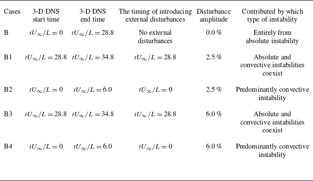
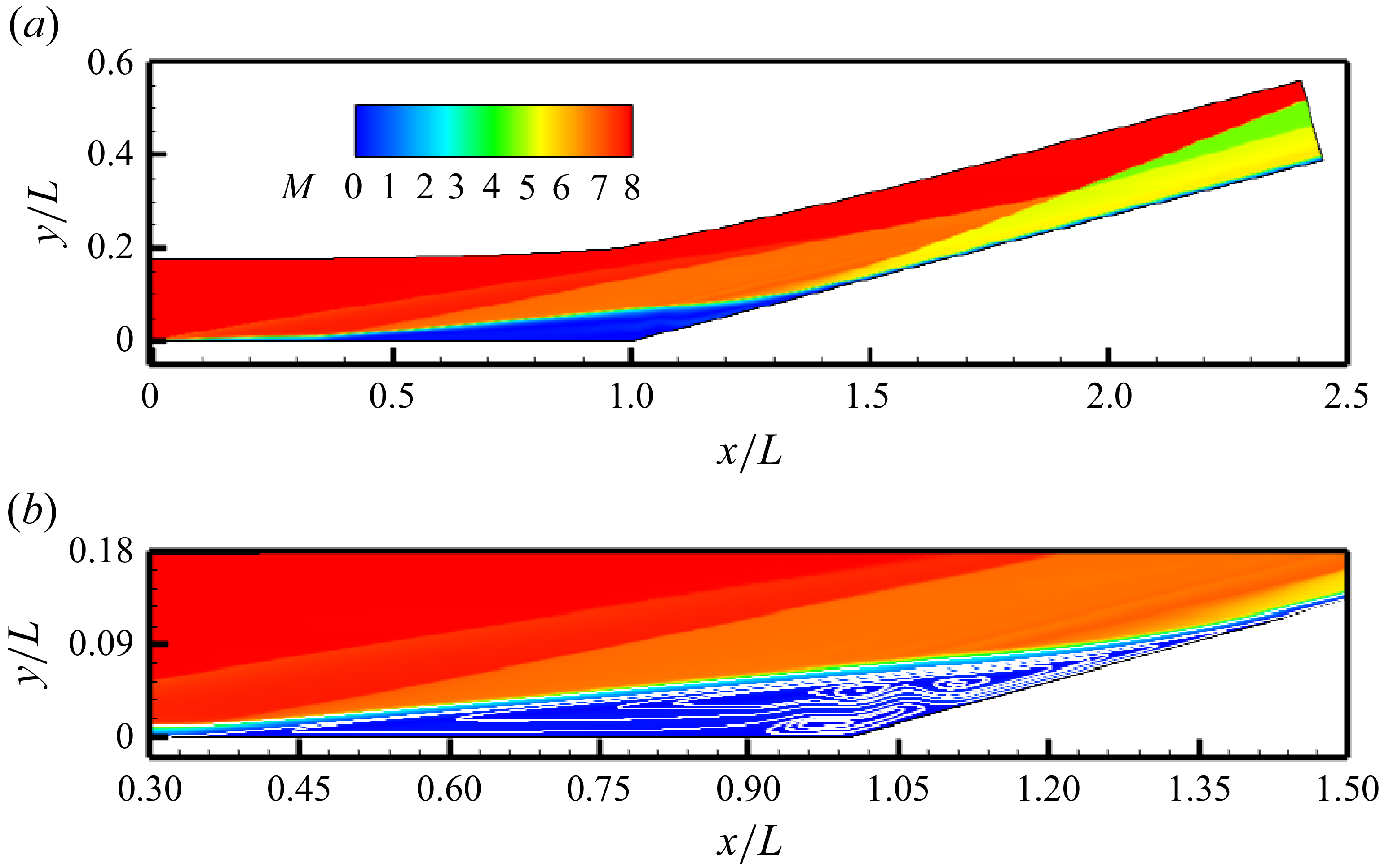
 a
 b

 a
 tU∞/L=3.2
 b
 tU∞/L=14.4
 c
 tU∞/L=17.6
 d
 tU∞/L=20.8
 e
 tU∞/L=25.6
 Cf=0

 a
 Aw/As
 x/L=1.07
 c
 tU∞/L=6.0
 tU∞/L=7.0
 tU∞/L=17.6
 b
 St
 x/L=1.8
 z/L=0.126

 a
 b
 c
 λz/L=0.084
 λz
 λz/L=0.084
 λz/L=0.04833
 λz

 w/U∞=±0.0014
 tU∞/L=14.4
 z/L=0

 a
 w/U∞
 tU∞/L=14.4
 x
 y
 z/L=0.126
 b
 w^/U∞
 λz/L=0.084
 c
 w/U∞
 y
 z
 x/L=1.07
 a

 x
 z
 yn/L=0.005
 a
 b
 tU∞/L=8.0
 tU∞/L=20.8
 yn

 a
 b
 c
 x/L=1.1
 x/L=1.5
 z/L=0.126
 yn/L=0.005

 a
 βL≈260.8
 ωrL/U∞
 βL=0
 ωrL/U∞≈135
 b
 βL=260.8


 a
 St′rms
 St′rms=4×10⁻³
 b
 St′rms

 Q
 u/U∞
 z/L=0
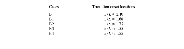

 Q
 u/U∞
 z/L=0

 Q
 u/U∞
 z/L=0

 Q
 u/U∞
 z/L=0

 St
 x
 z
 x/L
 a
 b
 λz/L≈0.084
 λz≈4.2
 λz/L≈0.042
 λz≈2.1

 St
 x
 z
 λz
 x/L=1.5
 a
 b

 St
 x
 z
 x/L
 a
 b
 c
 ωr=2πf

 x
 z
 x/L
 a
 b
 c
 f≈6
 ωr=2πf

 St
 x
 z
 x/L
 a
 b
 λz/L≈0.024
 λz≈1.2

 St
 x
 z
 λz
 x/L=1.5
 a
 b

 St
 x
 z
 x/L
 a
 b
 ωr=2πf

 x
 z
 x/L
 a
 b
 ωr=2πf

 a
 w^/U∞
 λz/L=0.084
 b
 x
 y
 f=0

 x
 y
 f=23
 a
 b
 c
 d
 e

 (w/U∞)max
 x/L
 f=23
 a
 b
 c
 d
 e

 x
 y
 f=114
 a
 b
 c
 d
 e

 x
 y
 f=503
 a
 b
 c
 d
 e

 a
 b

 λz=4.2 mm
 Nx×Ny=1750×240
 Nx×Ny=2240×320

 z/L=0.126
 yn/L=0.005
 a
 x/L=1.8
 b
 x/L=2.10
 c
 x/L=2.3
 d
 x/L=2.443

 Q
 u/U∞
 z/L=0

 a
 b
 St′rms
 St′rms=4×10⁻³
 c
 St′rms

 z/L=0
 a
 b
 c
 d

 a
 x/L=2.3
 b
 x/L=2.3

 x
 y
 a
 b
 c
 d
 e


