

1 Introduction
Under-expanded supersonic jets form when the static pressure at a choked nozzle exit is higher than the ambient pressure. Their applications in engineering range from exhausts of aircraft and rockets to mixing processes in supersonic combustors, accidental leakage of pressurised fluids and advanced cold-spray additive manufacturing processes such as the cold-spray process (Li et al. Reference Li, Muddle, Jahedi and Soria2012). Under-expanded jets have been the subject of intense research since they were first described theoretically by Prandtl and his Göttingen group (Prandtl Reference Prandtl1904, Reference Prandtl1907, Reference Prandtl1913; Ackeret Reference Ackeret, Ackeret, Betz, Forchheimer, Gyemant, Hopf, Lagally and Grammel1927). The acoustic-flow instability associated with an under-expanded supersonic impinging jet is known to cause self-sustained oscillations (Henderson Reference Henderson1966; Donaldson et al. Reference Donaldson and Snedeker1971). The high level of oscillations on the impinged surface can damage the surface structure and lead to material fatigue, while in advanced cold-spray manufacturing, high-amplitude pressure oscillations affect the quality of the deposited coating. Such oscillations have been observed in other configurations, for instance, subsonic impinging jets (Ho & Nosseir Reference Ho and Nosseir1981; Tam & Ahuja Reference Tam and Ahuja1990), a resonance tube, an edge-tone and a plate with a cavity (Raman & Srinivasan Reference Raman and Srinivasan2009). Many of the aspects associated with the self-sustained nature of the oscillations in these flows have been analysed and predicted in the context of linear dynamics (Hammond & Redekopp Reference Hammond and Redekopp1997; Haddad & Corke Reference Haddad and Corke1998; Erturk & Corke Reference Erturk and Corke2001; Wanderley & Corke Reference Wanderley and Corke2001; Pier Reference Pier2002; Barkley Reference Barkley2006; Sipp & Lebedev Reference Sipp and Lebedev2007; Mittal Reference Mittal2008; Oberleithner, Rukes & Soria Reference Oberleithner, Rukes and Soria2014; Sartor et al. Reference Sartor, Mettot, Bur and Sipp2015; Turton, Tuckerman & Barkley Reference Turton, Tuckerman and Barkley2015; Beneddine et al. Reference Beneddine, Sipp, Arnault, Dandois and Lesshafft2016; Ruban, Bernots & Kravtsova Reference Ruban, Bernots and Kravtsova2016; Illingworth, Monty & Marusic Reference Illingworth, Monty and Marusic2018). A linear dynamics approach is also the approach that we have utilised in the present study.
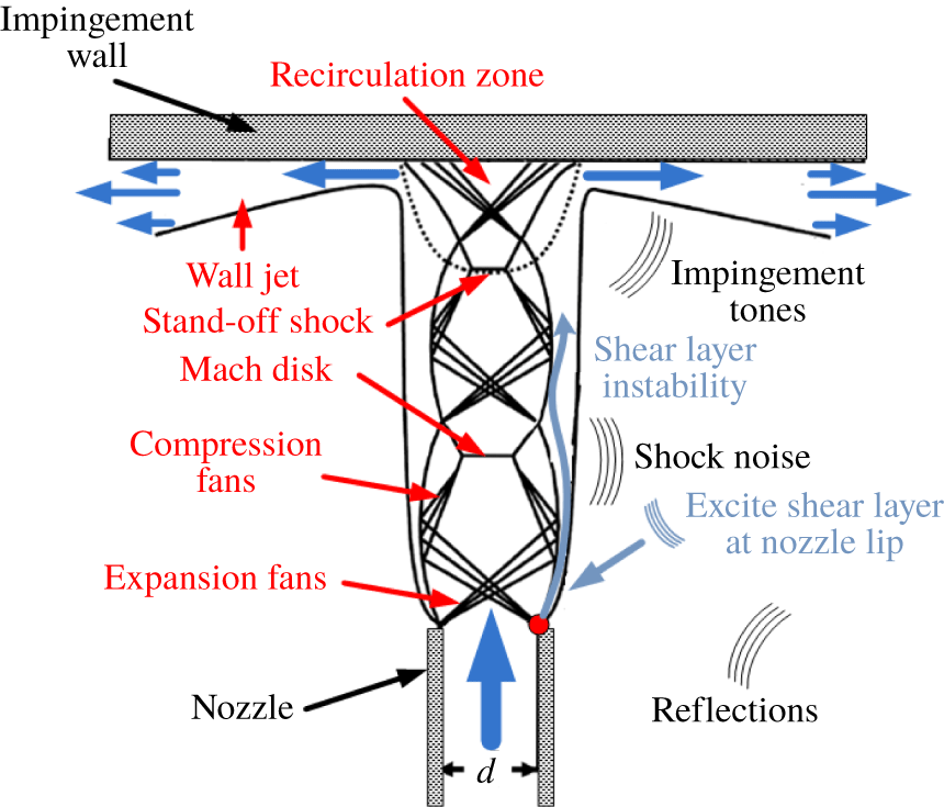
The accepted conceptual theory describing the feedback oscillations in supersonic impinging jets is due to Powell (Reference Powell1988), which is an analogue of the Rossiter mechanism found in open-cavity flow (Rossiter Reference Rossiter1964). The feedback loop is based on the interactions between the aero-acoustic field, which in under-expanded supersonic jet flows has a number of sources as depicted in figure 1, and the jet flow as evidenced in the ultrahigh-speed flow visualisation of Risborg & Soria (Reference Risborg, Soria, Kleine and Guillen2009) and Soria & Risborg (Reference Soria and Risborg2019). As can be clearly evidenced in these ultrahigh-speed schlieren visualisations, shear-layer disturbances develop in the form of Kelvin–Helmholtz (K–H) instabilities as shown diagrammatically by the blue arrow in the shear layer of the jet depicted in figure 1, which subsequently interact with the oblique shock, Mach disk and stand-off shock. These interactions displace the shocks, creating high-intensity acoustic waves at the shock locations and impinging region, as shown in figure 1, which travel upstream towards the jet orifice via the quiescent flow domain outside of the supersonic jet. As the circumferential edge of the jet expands upon exit from the nozzle in an under-expanded supersonic jet, some or all of these acoustic waves are blocked from directly reaching the jet nozzle lip. However, the acoustic waves are also reflected by the surrounding structures and the reflected waves can reach the nozzle lip and can be internalised into the initial conditions for a shear-layer instability at the nozzle lip via a receptivity mechanism, and hence close the feedback loop. Clear visualisation of this process can be observed in figure 11 of Risborg & Soria (Reference Risborg, Soria, Kleine and Guillen2009) and the corresponding ultrahigh-speed movie in Soria & Risborg (Reference Soria and Risborg2019).
Schematic of an under-expanded supersonic impinging jet.

Considerable evidence for the feedback loop being the mechanism responsible for the self-sustained oscillations has been accumulated via many experimental studies of supersonic impinging jets (Henderson & Powell Reference Henderson and Powell1993; Henderson, Bridges & Wernet Reference Henderson, Bridges and Wernet2005; Risborg & Soria Reference Risborg, Soria, Kleine and Guillen2009; Mason-Smith et al. Reference Mason-Smith, Edgington-Mitchell, Buchmann, Honnery and Soria2015; Soria & Risborg Reference Soria and Risborg2019). However, our understanding of the feedback loop ingredients is not complete, particularly from a quantitative point of view. The forward and backward paths of the feedback loop are a flow instability in the shear layer of the jet and an acoustic wave propagating in the medium, respectively. The flow instabilities subsequently develop into large-scale coherent vortical structures in the shear layer of the jet. The downstream convection of these structures has been observed in many experimental and numerical studies of free and impinging under-expanded supersonic jets (Powell Reference Powell1988; Edgington-Mitchell et al. Reference Edgington-Mitchell, Oberleithner, Honnery and Soria2014b; Gojon, Bogey & Marsden Reference Gojon, Bogey and Marsden2015; Mason-Smith et al. Reference Mason-Smith, Edgington-Mitchell, Buchmann, Honnery and Soria2015; Stegeman, Ooi & Soria Reference Stegeman, Ooi and Soria2015; Amili et al. Reference Amili, Edgington-Mitchell, Honnery and Soria2016; Gojon & Bogey Reference Gojon and Bogey2017). A prevailing belief is that the acoustic waves scattered by the nozzle lip are the sources that drive the convective K–H instability, which subsequently develop into these coherent structures (Henderson et al. Reference Henderson, Bridges and Wernet2005; Powell Reference Powell1988). However, to date, the mechanism that converts irrotational acoustic waves into the initial condition for the convective K–H instabilities at the jet nozzle in terms of the flow geometry and parameters of the supersonic under-expanded impinging jets has not been quantitatively analysed. This mechanism is clearly one which falls within the realms of the term receptivity as coined by Morkovin (Reference Morkovin1969) and Reshotko (Reference Reshotko1984) and defined as the internalisation of an external disturbance into the initial condition that either initiates or sustains a vortical fluid dynamic instability. In the context of this study, this process can be most visually observed in figure 11 of Risborg & Soria (Reference Risborg, Soria, Kleine and Guillen2009) and the corresponding ultrahigh-speed movie in Soria & Risborg (Reference Soria and Risborg2019), which clearly shows the initial condition of a K–H instability in the shear layer when the acoustic wave hits the jet lip closest for an inclined plate in an under-expanded supersonic jet impinging on an inclined plate.
Receptivity in a number of flows has been studied since the early 1970s with a heavy concentration on boundary-layer receptivity (Jones & Morgan Reference Jones and Morgan1972, Reference Jones and Morgan1973; Morgan Reference Morgan1974; Bechert Reference Bechert1988; Bechert & Stahl Reference Bechert and Stahl1988; Kerschen Reference Kerschen1996; Haddad & Corke Reference Haddad and Corke1998; Erturk & Corke Reference Erturk and Corke2001; Wanderley & Corke Reference Wanderley and Corke2001; Ruban et al. Reference Ruban, Bernots and Kravtsova2016). In addition, most of the other studies have been associated with the trailing-edge flow from a splitter plate where a simple vortex-sheet model with an infinite-extent splitter plate was considered. Kerschen (Reference Kerschen1996) studied the sensitivity of shear-layer instability waves formed at the trailing edge of a splitter plate to acoustic source location using a vortex-sheet model. Acoustic sources near and far from the trailing edge on both sides of the splitter plate were considered. The flow on one side of the splitter plate was quiescent, while it was either supersonic or subsonic on the other side of the plate. That study found that the development of shear-layer instability waves is more sensitive to the excitation on the flow side of the splitter plate compared to the excitation on the quiescent side of the plate. It was also observed that the receptivity to these acoustic disturbances decreases as the acoustic source location is moved away from the trailing edge. The influences of the sharpness of the leading edge and angle of acoustic incident were studied by Haddad & Corke (Reference Haddad and Corke1998) and Erturk & Corke (Reference Erturk and Corke2001) using the linearised Navier–Stokes equations. It was found that the leading-edge receptivity increases with the sharpness of the leading edge.
Tam (Reference Tam1986) proposed that for a two-dimensional shear layer developing from a splitter plate, a necessary condition for the reception of acoustic waves by the lip of the splitter plate, and hence the formation of K–H instabilities, was that the spatial wavenumber and temporal frequency of the shear-layer instability and the acoustic wave must match. Barone & Lele (Reference Barone and Lele2005) utilised the linearised Navier–Stokes equations with small-amplitude mass, momentum and heat sources in the vicinity of a mixing layer to study the receptivity of a compressible mixing layer. That study showed that not only does the receptivity depend on the frequency and the location of the excitation source but it also depends on the source type. The primary focus of these prior studies of receptivity has been confined to the relatively simple configuration of the mixing layer subjected to forcing via an external source, with only a few studies related to self-sustained flows (Rowley, Colonius & Basu Reference Rowley, Colonius and Basu2002). In the study by Rowley et al. (Reference Rowley, Colonius and Basu2002), the frequency dependence of the receptivity, which occurs at the upstream edge of the cavity of the self-sustained flow over a rectangular cavity, was ignored. This assumption as stated by Rowley (Reference Rowley2002) was considered ‘a crude model’.
As pointed out, numerous experimental and numerical studies of supersonic impinging jets have been conducted, the focus of these studies being on the large coherent structures with little attention paid to the initial mechanism that leads to the generation of the instability that subsequently evolves into these large-scale coherent vortical structures. To the best of our knowledge, the receptivity of under-expanded supersonic free or impinging jets has not previously been investigated. Hence, the primary objective of this paper is to address this gap by analysing the receptivity in under-expanded supersonic impinging jets. To achieve this goal, this paper seeks to quantify the transfer function of the receptivity and its dependency on location, frequency and azimuthal mode number of the acoustic source.
The paper is organised as follows. In § 2, the framework of the receptivity analysis within the structure of the linearised Navier–Stokes equations is presented. The mean flow required for the linearised Navier–Stokes equations is the mean flow obtained from large-eddy simulation (LES) of under-expanded supersonic impinging jets and is presented in § 3. The results including the mean flow fields and a comprehensive discussion of the receptivity, which is the primary focus of this study, and interpretation of the results are presented in § 4. Concluding remarks are presented in § 5.
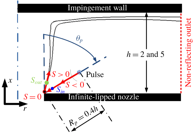
Schematic of the impinging jet with relevant parameters of the receptivity analysis. (Impulse is located within a radius of  $R_{p}=0.4h$ from the nozzle and angle of
 $\unicode[STIX]{x1D703}_{p}$ from the jet axis. The black solid line represents the sonic line in a typical under-expanded supersonic jet.)

2 Framework of the receptivity analysis
The aim of the receptivity analysis is to quantify the system response to external forcing. As stated above, receptivity in this case is defined as the internalisation of acoustic waves into the initial condition of the shear-layer instabilities at the sharp edge of the nozzle lip. Therefore, there is a need to quantify the acoustic irrotational field and vortical fluid flow field in the limit as the sharp edge of the nozzle lip is approached, i.e. as the point  $s=0$ in figure 2 is approached from
 $s_{in}$ and
 $s_{out}$, respectively. The receptivity in this context is characterised by a transfer function at the nozzle lip, which is defined as the ratio of the output energy of the rotational flow to the input acoustic irrotational energy in the limit where the locations of both these energies approach the point
 $s=0$, i.e. the nozzle lip. Therefore, the lip of the nozzle can be considered a linear transformer, because receptivity is considered to be linear (Haddad & Corke Reference Haddad and Corke1998; Erturk & Corke Reference Erturk and Corke2001). This permits us to employ the linearised Navier–Stokes equations to quantitatively study the receptivity in under-expanded supersonic impinging jet flows.
Modal linear stability theory has been used widely in the past to reveal the underpinning physics of unsteady flows (Hammond & Redekopp Reference Hammond and Redekopp1997; Pier Reference Pier2002; Barkley Reference Barkley2006; Sipp & Lebedev Reference Sipp and Lebedev2007; Mittal Reference Mittal2008; Oberleithner et al. Reference Oberleithner, Rukes and Soria2014; Sartor et al. Reference Sartor, Mettot, Bur and Sipp2015; Turton et al. Reference Turton, Tuckerman and Barkley2015; Beneddine et al. Reference Beneddine, Sipp, Arnault, Dandois and Lesshafft2016; Illingworth et al. Reference Illingworth, Monty and Marusic2018). Receptivity, however, as pointed out by Reshotko (Reference Reshotko1976), is different from instability both physically and mathematically. It is a transformation of acoustic irrotational disturbances into vortical fluid dynamic instabilities. The problem is not homogeneous and a normal mode analysis (i.e. eigenvalue problem) cannot be used. Instead the solution of the linearised Navier–Stokes equations with external forcing is required (Reshotko Reference Reshotko1976). This assumption is consistent with that used in the previous studies of leading-edge receptivity (Haddad & Corke Reference Haddad and Corke1998; Erturk & Corke Reference Erturk and Corke2001) where the receptivity is considered to be a linear process for weak disturbances that permits the application of the linearised Navier–Stokes equations in the analysis.
The linearised compressible Navier–Stokes equations are derived by superimposing small-amplitude disturbances on a mean flow. Denoting the mean flow variables as  $\overline{(\cdots \,)}$ and perturbations as
 $(\cdots \,)^{\prime }$, the linearised compressible Navier–Stokes equations are given as
 $$\begin{eqnarray}\left.\begin{array}{@{}c@{}}{\displaystyle \frac{\unicode[STIX]{x2202}\unicode[STIX]{x1D70C}^{\prime }}{\unicode[STIX]{x2202}t}}=-\unicode[STIX]{x1D735}\boldsymbol{\cdot }\left(\unicode[STIX]{x1D70C}\boldsymbol{u}\right)^{\prime },\\ {\displaystyle \frac{\unicode[STIX]{x2202}\left(\unicode[STIX]{x1D70C}\boldsymbol{u}\right)^{\prime }}{\unicode[STIX]{x2202}t}}=-\unicode[STIX]{x1D735}\boldsymbol{\cdot }\left(\overline{\unicode[STIX]{x1D70C}\boldsymbol{u}}\otimes \boldsymbol{u}^{\prime }+(\unicode[STIX]{x1D70C}\boldsymbol{u})^{\prime }\otimes \overline{\boldsymbol{u}}\right)-\unicode[STIX]{x1D735}p^{\prime }+\overline{\unicode[STIX]{x1D707}}\unicode[STIX]{x1D735}\boldsymbol{\cdot }\mathbb{T}^{\prime },\\[10.0pt] {\displaystyle \frac{\unicode[STIX]{x2202}\left(\unicode[STIX]{x1D70C}e\right)^{\prime }}{\unicode[STIX]{x2202}t}}=-\unicode[STIX]{x1D735}\boldsymbol{\cdot }\left(\overline{(\unicode[STIX]{x1D70C}e+p)}\boldsymbol{u}^{\prime }+(\unicode[STIX]{x1D70C}e+p)^{\prime }\overline{\boldsymbol{u}}\right)+\overline{k}\unicode[STIX]{x1D6FB}^{2}T^{\prime }+\overline{\unicode[STIX]{x1D707}}V_{KE},\end{array}\right\}\end{eqnarray}$$
where
 $$\begin{eqnarray}\left.\begin{array}{@{}c@{}}V_{KE}=\left(\left(\unicode[STIX]{x1D735}\boldsymbol{\cdot }\mathbb{T}^{\prime }\right)\boldsymbol{\cdot }\overline{\boldsymbol{u}}+\left(\unicode[STIX]{x1D735}\boldsymbol{\cdot }\mathbb{T}^{\prime }\right)\boldsymbol{\cdot }\boldsymbol{u}^{\prime }+\mathbb{T}^{\prime }:\unicode[STIX]{x1D735}\overline{\boldsymbol{u}}+\overline{\mathbb{T}}:\unicode[STIX]{x1D735}\boldsymbol{u}^{\prime }\right),\\ \mathbb{T}=\unicode[STIX]{x1D735}\boldsymbol{u}+\left(\unicode[STIX]{x1D735}\boldsymbol{u}\right)^{\text{T}}-\frac{2}{3}\left(\unicode[STIX]{x1D735}\boldsymbol{\cdot }\boldsymbol{u}\right)\mathbb{I},\end{array}\right\}\end{eqnarray}$$
and the linearised version of the equation of state is
 $$\begin{eqnarray}\displaystyle p^{\prime }={\displaystyle \frac{\overline{\unicode[STIX]{x1D70C}}T^{\prime }+\unicode[STIX]{x1D70C}^{\prime }\overline{T}}{\unicode[STIX]{x1D6FE}}}. & & \displaystyle\end{eqnarray}$$
Finally, the viscosity and thermal conductivity are given by
 $$\begin{eqnarray}\overline{\unicode[STIX]{x1D707}}={\displaystyle \frac{\overline{T}^{\,0.76}}{\mathit{Re}}}\quad \text{and}\quad \overline{k}={\displaystyle \frac{\overline{\unicode[STIX]{x1D707}}}{\unicode[STIX]{x1D6FE}-1}}{\displaystyle \frac{1}{Pr}}.\end{eqnarray}$$
These equations are commonly presented in the concise matrix form
 $$\begin{eqnarray}\displaystyle {\displaystyle \frac{\unicode[STIX]{x2202}q^{\prime }}{\unicode[STIX]{x2202}t}}=\mathbb{A}q^{\prime }, & & \displaystyle\end{eqnarray}$$
where  $q^{\prime }$ represents the perturbations (
 $\unicode[STIX]{x1D70C}^{\prime },u_{x}^{\prime },u_{r}^{\prime },u_{\unicode[STIX]{x1D703}}^{\prime },e^{\prime }$) and
 $\mathbb{A}$ is the linear operator advancing the small perturbations in time.
The above equations are non-dimensionalised as follows with the superscript ‘*’ representing dimensional values, while the subscript ‘ $o$’ refers to ambient conditions:
 $$\begin{eqnarray}\left.\begin{array}{@{}c@{}}x_{j}={\displaystyle \frac{x_{j}^{\ast }}{d}},\quad U_{j}={\displaystyle \frac{U_{j}^{\ast }}{a_{o}^{\ast }}},\quad \unicode[STIX]{x1D70C}={\displaystyle \frac{\unicode[STIX]{x1D70C}^{\ast }}{\unicode[STIX]{x1D70C}_{o}^{\ast }}},\quad t={\displaystyle \frac{t^{\ast }a_{o}^{\ast }}{d}},\quad p={\displaystyle \frac{p^{\ast }}{\unicode[STIX]{x1D70C}_{o}^{\ast }a_{o}^{\ast 2}}},\\ T={\displaystyle \frac{T^{\ast }}{\unicode[STIX]{x1D6FE}T_{o}^{\ast }}},\quad \unicode[STIX]{x1D707}={\displaystyle \frac{\unicode[STIX]{x1D707}^{\ast }}{Re\unicode[STIX]{x1D707}_{o}^{\ast }}},\quad Pr={\displaystyle \frac{\unicode[STIX]{x1D710}^{\ast }}{\unicode[STIX]{x1D6FC}^{\ast }}},\quad Re={\displaystyle \frac{\unicode[STIX]{x1D70C}_{o}^{\ast }a_{o}^{\ast }d}{\unicode[STIX]{x1D707}_{o}^{\ast }}}\quad St=fd/a_{o}^{\ast }.\end{array}\right\}\end{eqnarray}$$
In these equations,  $x_{j}$ represents the spatial vector,
 $d$ the jet diameter,
 $U_{j}$ the velocity vector,
 $a$ the speed of sound,
 $\unicode[STIX]{x1D70C}$ the density,
 $T$ the temperature,
 $t$ time (acoustic time unit),
 $p$ the pressure,
 $\unicode[STIX]{x1D6FE}$ the heat capacity ratio,
 $f$ the frequency,
 $St$ the Strouhal number and
 $\unicode[STIX]{x1D707}$ the dynamic viscosity, which is given by
 $\unicode[STIX]{x1D707}/\unicode[STIX]{x1D707}_{o}=(T/T_{o})^{0.7}$. (Note that the acoustic time unit in the configuration of this study is equivalent to the characteristic time of a jet flow based on the inlet velocity and jet diameter as the nozzle is choked in under-expanded supersonic jets; hence the inlet Mach number is unity.) The variable
 $Re$ represents the Reynolds number and
 $Pr$ the Prandtl number.
The configuration of the under-expanded impinging jet is characterised by a nozzle-to-wall distance denoted by  $h$. The jets emanate from an infinite-lipped nozzle (i.e. a circular hole in a flat plate) which is referred to as the nozzle lip throughout the rest of the paper. An acoustic impulse described by
 $$\begin{eqnarray}\displaystyle p^{\prime }(t=0)=A\;\exp \left(-{\displaystyle \frac{(x-x_{o})^{2}}{2\unicode[STIX]{x1D70E}_{x}^{2}}}-{\displaystyle \frac{(r-r_{o})^{2}}{2\unicode[STIX]{x1D70E}_{r}^{2}}}\right)\cos (2\unicode[STIX]{x03C0}m\unicode[STIX]{x1D703}) & & \displaystyle\end{eqnarray}$$
is used as a localised initial condition of the acoustic irrotational pressure fluctuations, where  $A$ is the amplitude of the impulse;
 $x_{o}$ and
 $r_{o}$ are the streamwise and radial locations of the centre of the impulse, respectively;
 $\unicode[STIX]{x1D70E}_{x}$ and
 $\unicode[STIX]{x1D70E}_{r}$ are the radii of the impulse in the streamwise and radial directions, respectively, with
 $\unicode[STIX]{x1D70E}_{x}$ and
 $\unicode[STIX]{x1D70E}_{r}\ll \unicode[STIX]{x1D706}$ the acoustic wavelength; and
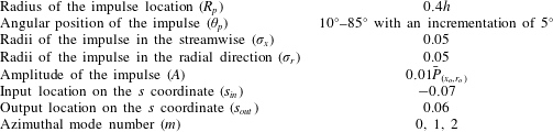
 $m$ is the azimuthal mode number. To study the sensitivity of amplification of the incoming wave at the nozzle lip to the impulse location, the centre of the impulse is located at a radius of
 $R_{p}=0.4h$ from the nozzle lip and an angle of
 $\unicode[STIX]{x1D703}_{p}$, where
 $\unicode[STIX]{x1D703}_{p}$ is the angle from the jet axis as shown in figure 2. This corresponds to the location of the impulse in the axial and the radial directions of
 $x_{o}=R_{p}\sin (\unicode[STIX]{x1D703}_{p})$ and
 $r_{o}=R_{p}\cos (\unicode[STIX]{x1D703}_{p})$. Full details of the under-expanded supersonic impinging jet configuration are presented in figure 2. Radius
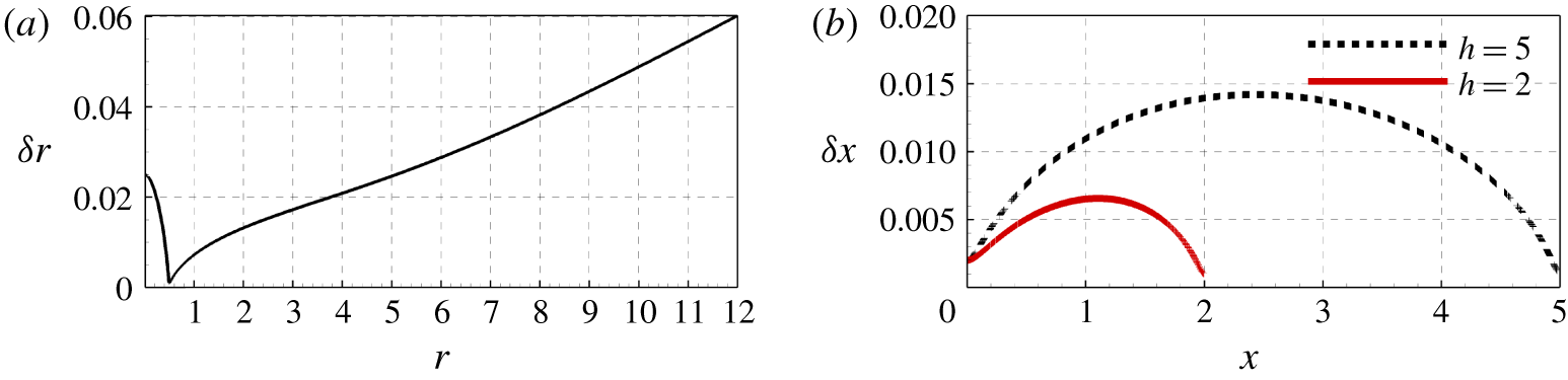
 $R_{p}=0.4h$ is chosen to maintain an adequate resolution of the propagating wave as a stretched grid is used in the radial direction (see figure 6) and to obtain well-separated input and output signals with no overlap for the purpose of the receptivity analysis.
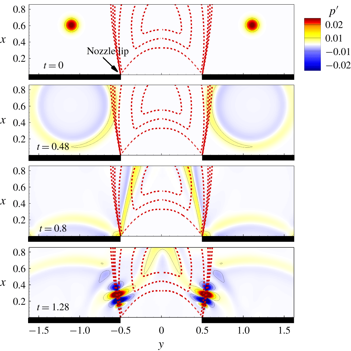
Using a mean flow field, the linearised Navier–Stokes equations can be solved to obtain the time evolution of the flow disturbances to the impulse. The time evolution of perturbations for the case where the impulse is located at  $\unicode[STIX]{x1D703}_{p}=45^{\circ }$ is presented in figure 3. The initial condition (
 $t=0$) is started by a pressure impulse. The pressure wave formed by the impulse travels in the medium and reaches the nozzle lip at
 $t=0.8$. It is internalised into a shear-layer instability and forms a convective instability as shown in figure 3 at
 $t=1.28$.
Instantaneous contours of the pressure fluctuation field of the pressure impulse simulation for a nozzle-to-wall distance of  $2$ jet diameters, where the impulse is located at
 $R_{p}=0.8$ and
 $\unicode[STIX]{x1D703}_{p}=45^{\circ }$ (
 $y$ is related to radius by
 $-r<y<r$).

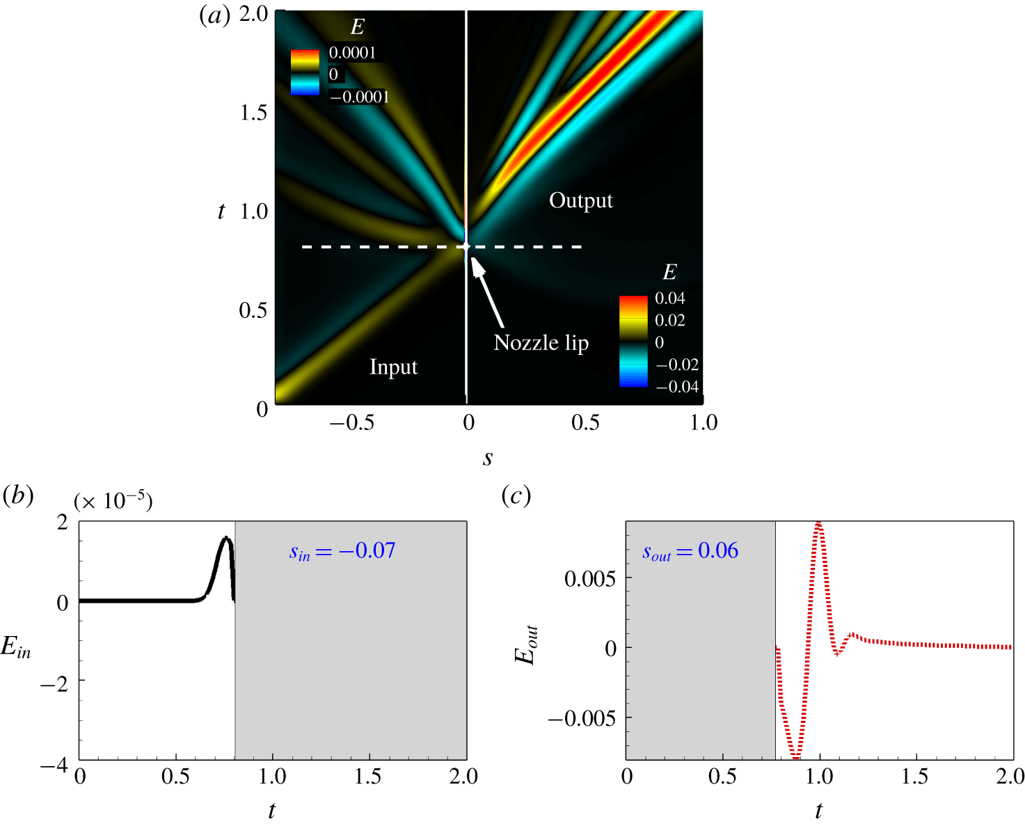
(a) The signal history on new coordinate  $s$ (the colourmaps of input signal (
 $s<0$) and output signal (
 $s>0$) are adjusted as shown at top-left and bottom-right corners, respectively). (b) Input and (c) output signals with relevant time cut-off for the case with a nozzle-to-wall distance of two jet diameters for the same case as in figure 3.

To obtain a better understanding of the receptivity process, the transfer function between the input and output energy of the disturbance at the nozzle lip is required. The input is located on the straight line connecting the source to the nozzle lip (blue dot marked on  $s_{in}$ in figure 2) and the output is located in the shear layer of the jet as close as possible to the nozzle lip (green dot marked on
 $s_{out}$ in figure 2). A new one-dimensional coordinate is defined as
 $s$. It is centred at the nozzle lip marked by
 $s=0$ in figure 2. Any location on the straight line from the nozzle lip to the impulse acoustic source has a negative sign increasing towards the source location (
 $s<0$) and any location at the shear layer has a positive sign in this coordinate which is increasing by moving away from the nozzle lip (
 $s>0$). The fluctuation of the density-weighted kinetic energy of the disturbance is defined as
 $$\begin{eqnarray}\displaystyle E={\textstyle \frac{1}{2}}\left[2\overline{\unicode[STIX]{x1D70C}}\overline{u_{i}}u_{i}^{\prime }+\overline{\unicode[STIX]{x1D70C}}{u_{i}^{\prime }}^{2}+\unicode[STIX]{x1D70C}^{\prime }\overline{u_{i}}^{2}+2\unicode[STIX]{x1D70C}^{\prime }u_{i}^{\prime }\overline{u_{i}}+\unicode[STIX]{x1D70C}^{\prime }{u_{i}^{\prime }}^{2}\right]. & & \displaystyle\end{eqnarray}$$
The time history of  $E$ on the
 $s$ coordinate for the linearised simulation for a case with a pressure impulse at
 $R_{p}=0.8$ and
 $\unicode[STIX]{x1D703}_{p}=45^{\circ }$ is presented in figure 4(a). The white solid line provides the location of the nozzle lip,
 $s=0$, and the white dashed line shows the instance when the pressure wave, generated by the acoustic impulse, reaches the nozzle lip. Note that the colourbars of the left- and right-hand sides of the solid white line have different scales and adjusted for demonstration purposes, the acoustic energy is much smaller than the resulting fluid dynamic energy. The input signal must be sampled in the bottom-left quarter of this plot, while the output signal must be sampled in the top-right quarter of this plot. To obtain a representative form of the transfer function of the receptivity as per the definition, the acoustic energy and hydrodynamic energy must be evaluated as
 $s_{in}\rightarrow 0$ and
 $s_{out}\rightarrow 0$, respectively. However, the minimum values of
 $s_{in}$ and
 $s_{out}$ are limited by the ability to distinguish the input and output signals at the sample points which in turn is limited by the spatial resolution of the numerical grid. Therefore, the values of
 $s_{in}=-0.07$ and
 $s_{out}=0.06$ are selected in this analysis. (Note that these values are non-dimensionalised with respect to the jet diameter.) Typical input and output signals at
 $s_{in}$ and
 $s_{out}$ are presented in figure 4(b,c). Assuming a linear time-invariant relationship between the input and the output, the output can be predicted by a convolution along time between the input variable and a convolution kernel (Sasaki et al. Reference Sasaki, Vinuesa, Cavalieri, Schlatter and Henningson2019) given by
 $$\begin{eqnarray}\displaystyle E_{out}(t)=\int _{-\infty }^{\infty }g(\unicode[STIX]{x1D70F})E_{in}(t-\unicode[STIX]{x1D70F})\,\text{d}\unicode[STIX]{x1D70F}, & & \displaystyle\end{eqnarray}$$
where  $g(\unicode[STIX]{x1D70F})$ is the convolution kernel which is also referred to as a time-invariant transfer function. In order to obtain this convolution kernel, it is more convenient to formulate the problem in the frequency space. In the frequency domain, the frequency response can be obtained from the auto-spectrum of the input and cross-spectra between the input and output signals (Bendat & Piersol Reference Bendat and Piersol2011; Sasaki et al. Reference Sasaki, Vinuesa, Cavalieri, Schlatter and Henningson2019). Hence, the transfer function in the frequency domain is defined as
 $$\begin{eqnarray}\displaystyle G(St)={\displaystyle \frac{||\hat{E}_{out}(St)\hat{E}_{in}^{\ast }(St)||}{||\hat{E}_{in}(St)\hat{E}_{in}^{\ast }(St)||}}, & & \displaystyle\end{eqnarray}$$
where  $St$ is the Strouhal number and
 $\hat{E}$ is the Fourier transform of the fluctuations of the density-weighted kinetic energy of the flow.
In order to study the effect of the acoustic impulse location on the receptivity, the angular position of the acoustic impulse is varied from a position close to the impingement wall ( $\unicode[STIX]{x1D703}_{p}=10^{\circ }$) to one near the infinite-lipped nozzle wall (
 $\unicode[STIX]{x1D703}_{p}=85^{\circ }$) using angular increments of
 $5^{\circ }$. This study is limited to the first three azimuthal mode numbers as they are found to be the dominant modes based on previous studies (Weightman et al. Reference Weightman, Amili, Honnery, Edgington-Mitchell and Soria2019). Full details of all the parameters and their values for the receptivity analysis are presented in table 1.
Numerical and physical parameters of the receptivity analysis.

3 Large-eddy simulation – determination of the mean flow
An in-house parallel high-fidelity LES code with a novel shock identification and capturing method was used to undertake the necessary LES to determine the mean flow associated with the under-expanded supersonic impinging jet. The code, which has been tested and validated in previous studies (Stegeman et al. Reference Stegeman, Pèrez, Soria and Theofilis2016a; Stegeman, Soria & Ooi Reference Stegeman, Soria and Ooi2016b; Karami, Edgington-Mitchell & Soria Reference Karami, Edgington-Mitchell and Soria2018a; Karami et al. Reference Karami, Stegeman, Theofilis, Schmid and Soria2018b; Karami & Soria Reference Karami and Soria2018; Karami et al. Reference Karami, Stegeman, Ooi and Soria2019), solves the filtered compressible conservation equations of mass, momentum and total energy in cylindrical coordinates. The subgrid-scale terms are computed using Germano’s dynamic model with the adjustment proposed by Lilly (Reference Lilly1992). A sixth-order central finite-difference method is used for spatial discretisation in the smooth regions, while a fifth-order weighted essentially non-oscillating scheme with local Lax–Friedrichs flux splitting is used in the discontinuous regions. The temporal integration is performed using a fourth-order five-step Runge–Kutta scheme (Kennedy & Carpenter Reference Kennedy and Carpenter1994; Kennedy, Carpenter & Lewis Reference Kennedy, Carpenter and Lewis2000). The locally one-dimensional inviscid compressible boundary condition proposed by Poinsot & Lele (Reference Poinsot and Lele1992) is employed at the far-field outflow boundaries. For further details of the numerical method, the novel shock identification and capturing method and LES code, the interested reader is referred to Karami et al. (Reference Karami, Stegeman, Ooi and Soria2019).
The ratio between the stagnation pressure measured in the jet plenum and the ambient pressure, commonly referred to as the nozzle pressure ratio ( $\mathit{NPR}$), is 3.4 for all cases considered. This
 $\mathit{NPR}$ is higher than the critical
 $\mathit{NPR}$ (i.e. here for dry air the critical
 $\mathit{NPR}$ is 1.893); hence, the nozzle is choked and the nozzle exit Mach number is unity. Parameters addressed in the present work are guided by the recent experimental studies of under-expanded supersonic impinging jets of Mason-Smith et al. (Reference Mason-Smith, Edgington-Mitchell, Buchmann, Honnery and Soria2015) and Amili et al. (Reference Amili, Edgington-Mitchell, Honnery and Soria2016), who found that the
 $\mathit{NPR}$ of 3.4 leads to the initial formation of a small Mach disk. They also observed that an increase in the
 $\mathit{NPR}$ enlarges the size of the Mach disk. Hence, an
 $\mathit{NPR}$ of 3.4 was selected for this numerical study, as being the case where the Mach disk forms from the converging point between the expansion and compression waves.
Experimental and numerical studies of the same configuration (Ho & Nosseir Reference Ho and Nosseir1981; Dauptain, Cuenot & Gicquel Reference Dauptain, Cuenot and Gicquel2010) have shown that the instabilities in the shear layer are intensified when the nozzle-to-wall distance,  $h$, is shorter than the inviscid core of the jet. Considering this observation, in order to study the effect of nozzle-to-wall distance on the receptivity at the nozzle lip, two nozzle-to-wall distances of
 $2d$ and 5
 $d$ are investigated, which based on Ho & Nosseir (Reference Ho and Nosseir1981) and our numerical experiment lie within the potential core, which for a jet with an
 $\mathit{NPR}$ of 3.4 is larger than
 $7.5d$. The significance of the impinging plate located at
 $2d$ is that a dominant impingement tone was observed, while the significance of the impinging plate located at
 $5d$ is its potential to allow the spatial development of large structures and their interactions with the shocks.
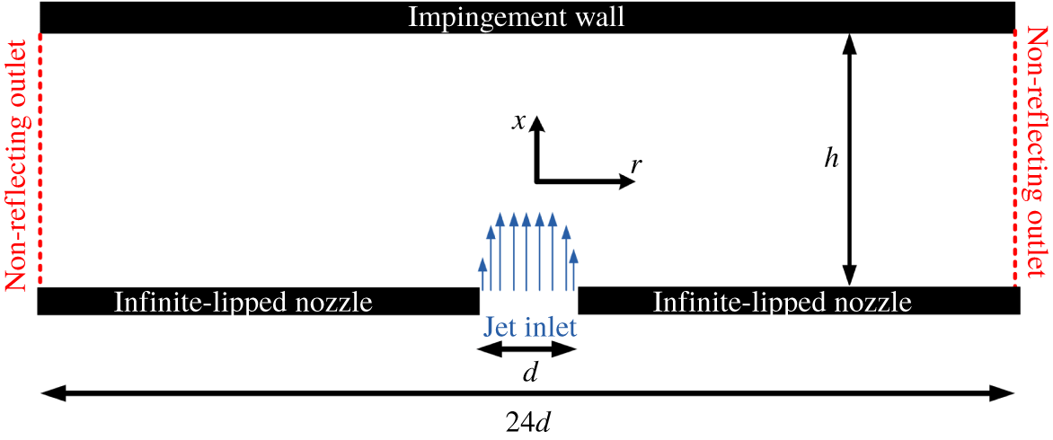
Schematic of the domain and the configuration of this study.

(a) Radial and (b) axial mesh spacing.

Computational grid of LES.

The size of the domain in the radial direction is  $12d$ (figure 5). The details of the computational grid for the two cases are provided in table 2. A uniform grid is employed in the azimuthal direction,
 $\unicode[STIX]{x1D703}$. In the axial direction,
 $x$, a fine grid is used near the nozzle and near the impingement wall. In the radial direction,
 $r$, a fine grid is used in the mixing-layer region with a polynomial stretching of the grid points towards the centre of the jet and the far field. The locations of the radial and axial grid points are shown in figure 6 for the sake of completeness. Note that the maximum mesh spacing of 0.04 for
 $r<8.5$ allows the capture of the propagation of acoustic waves with Strouhal number up to 5.0 in the LES. The mean inlet axial velocity
 $U_{in}$ is specified using the hyperbolic-tangent function used in the work of Bodony & Lele (Reference Bodony and Lele2005) with a non-dimensionalised inlet momentum thickness of
 $0.04$ which is comparable to that of previous studies (Bogey, Marsden & Bailly Reference Bogey, Marsden and Bailly2011). The inlet velocity is free of any synthetic turbulence in order to permit future comparison with experimental data as the experimental nozzles of the under-expanded supersonic impinging jet typically have a very high contraction ratio, which results in a very low turbulence level of the issuing jet (Edgington-Mitchell, Honnery & Soria Reference Edgington-Mitchell, Honnery and Soria2014a). The Reynolds number is 50 000 which is approximately an order of magnitude lower than that used in experimental studies. This Reynolds number is chosen to maintain the LES resolution requirement at acceptable computational cost (Kawai & Lele Reference Kawai and Lele2010).
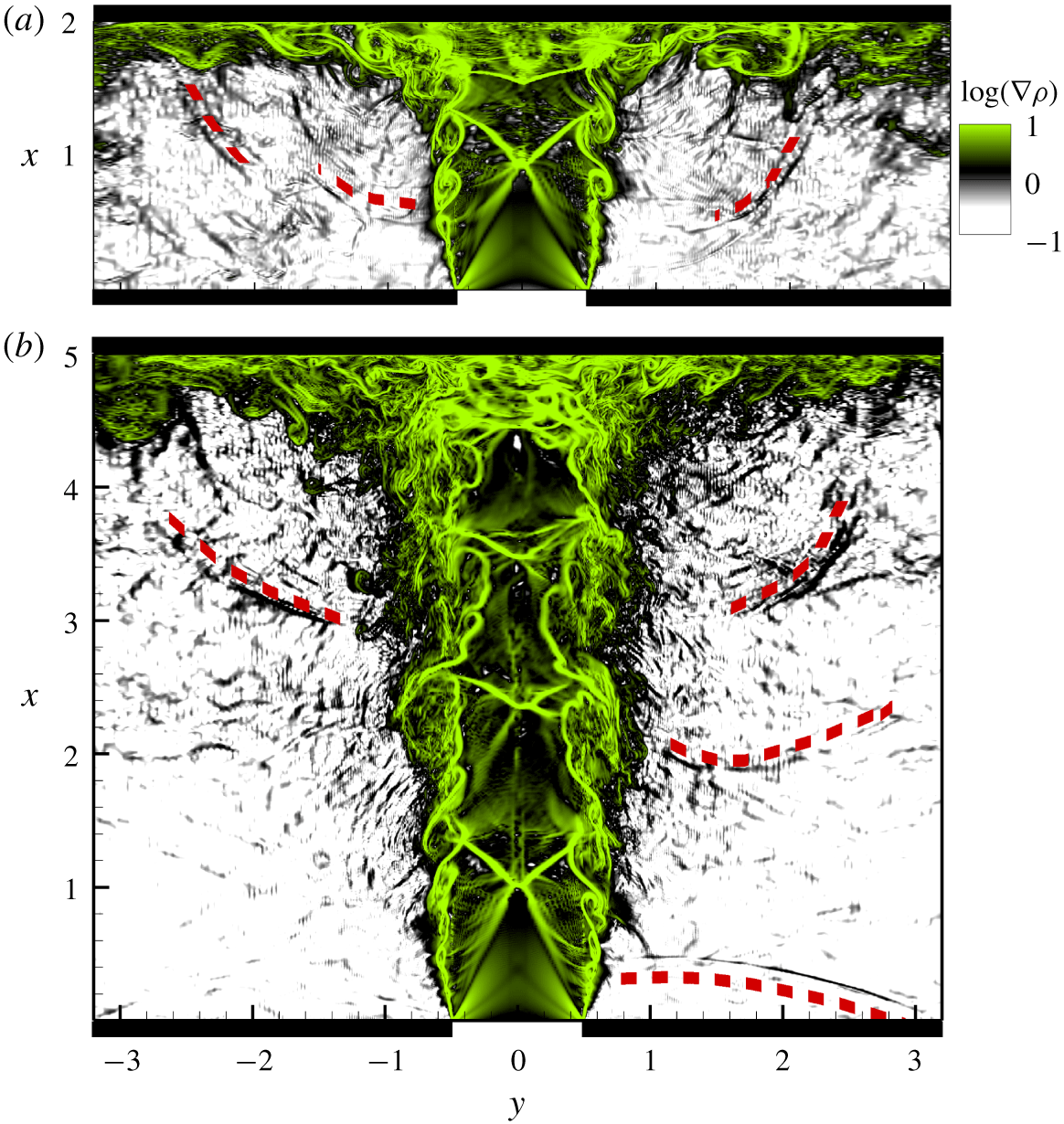
Figure 7 shows the contour maps of the instantaneous density-gradient field for the two cases of this study with nozzle-to-wall distances  $h=2d$ and
 $h=5d$, respectively. The development of instabilities in the shear layer as well as the travelling acoustic waves (i.e. the dashed red curves), which are two of the main components of the feedback loop in under-expanded supersonic impinging jets, are clearly observable. Furthermore, figure 7(b), the
 $h=5d$ case, clearly shows a reflected acoustic wave from the infinite lip. Before proceeding further, the interested reader may consult animations of the density gradients shown in figure 7, which are presented in the supplementary movies available at https://doi.org/10.1017/jfm.2020.63. These animations are quite instructive for gaining an overall picture of flow and acoustic paths.
Instantaneous contour plots of the density gradient for (a)  $h/d=2$ and (b)
 $h/d=5$ (
 $y$ is related to radius by
 $-r<y<r$).

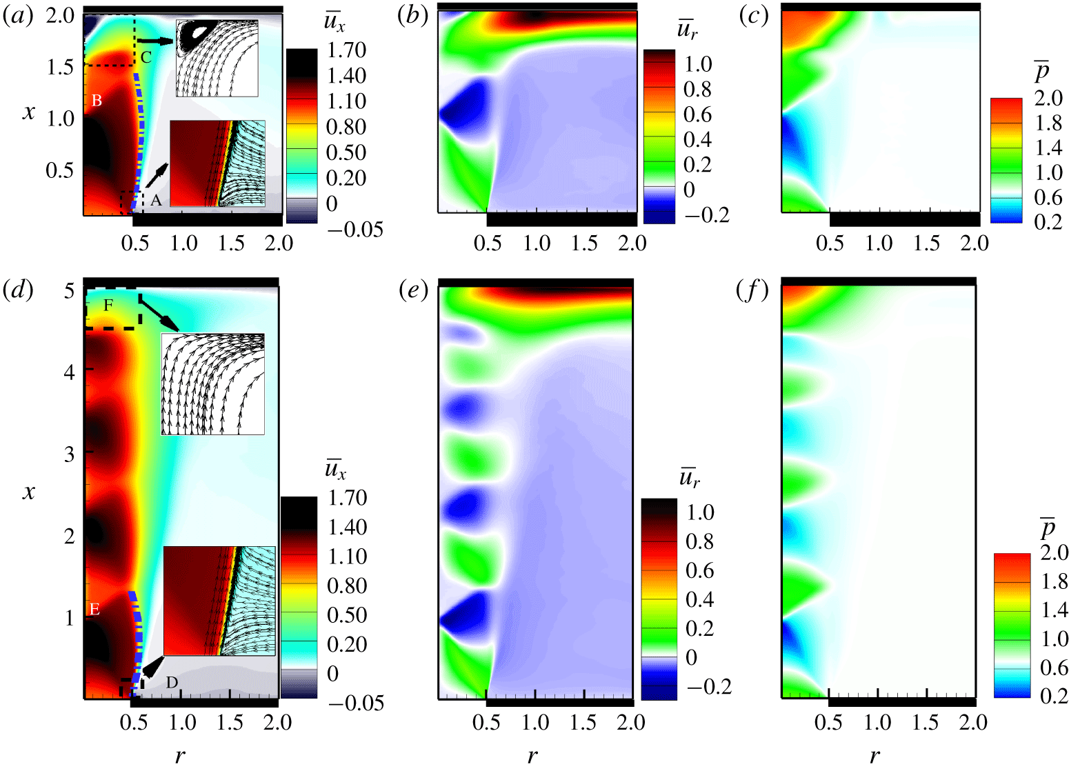
Ensemble-averaged (a,d) streamwise velocity, (b,e) radial velocity and (c,f) pressure for nozzle-to-wall distances of  $2d$ (a–c) and
 $5d$ (d–f).

4 Results and discussion
4.1 Mean flow fields
The linearised Navier–Stokes equations require a mean flow, which in this study is the mean flow field. The ensemble average of any non-dimensionalised variable  $\unicode[STIX]{x1D719}$ is computed as the temporal and azimuthal mean given by the following equation:
 $$\begin{eqnarray}\displaystyle \bar{\unicode[STIX]{x1D719}}(x,r)={\displaystyle \frac{1}{N_{t}\times N_{\unicode[STIX]{x1D703}}}}\mathop{\sum }_{i=1}^{N_{t}}\mathop{\sum }_{j=1}^{N_{\unicode[STIX]{x1D703}}}\unicode[STIX]{x1D719}(x,r,\unicode[STIX]{x1D703}_{j},t_{i}), & & \displaystyle\end{eqnarray}$$
where  $N_{t}$ is the number of snapshots over which the average is computed and
 $N_{\unicode[STIX]{x1D703}}$ is the number of azimuthal grids. The mean flow field for each case is obtained using (4.1) over 200 acoustic time units of the statistically stationary LES.
Figure 8 shows the contour plots of the ensemble-averaged axial and radial velocities, as well as ensemble-averaged pressure fields for  $h=2d$ and
 $h=5d$. Figure 8(a,d) shows the mean streamwise velocities. The streamlines are shown in the zoomed insets, near the nozzle exit and the impingement wall. The initial expansion of the shear layer upon exit from the nozzle is visible for both nozzle-to-wall distances. There is a high level of entrainment near the nozzle in the regions marked by ‘A’ and ‘D’ (figure 8a,d). This is clearer in the zoomed insets where the streamlines are visualised. The velocity vectors are directed perpendicularly towards the jet except very close to the nozzle where they move towards the nozzle and then close to the nozzle turn parallel to the jet edge into the jet direction. A small Mach disk with a size of less than 0.05 jet diameters is also noticed at
 $x$
 ${\approx}$ 1.0, marked by ‘B’ and ‘E’ in figure 8(a,d). The small size of the Mach disk is due to the low
 $\mathit{NPR}$ of 3.4 (Edgington-Mitchell et al. Reference Edgington-Mitchell, Oberleithner, Honnery and Soria2014b). Other classical features of an under-expanded supersonic jet such as a triple point and an oblique shock are also visible.
An evident expansion and contraction of the jet boundary are also observed, which are characteristic of under-expanded supersonic jets (Raman Reference Raman1997). An interesting parameter is the cell length (i.e. the wavelength of the wave-shape periphery of the jet as shown by dashed-dot blue curves in figure 8a,d). Prandtl (Reference Prandtl1904) proposed his well-known formula to approximate the cell length based on the small perturbation theory. This formula has a form of  $\unicode[STIX]{x1D706}/d=A\sqrt{(NPR-NPR_{c})}$, where
 $\unicode[STIX]{x1D706}$ is the cell length,
 $A$ is the model constant and
 $NPR_{c}$ is the critical
 $\mathit{NPR}$. He found a value of
 $1.22$ for the model constant
 $A$. Based on extensive measurement of cell lengths in photographs of choked jets, Emden (Reference Emden1899) proposed a value of
 $0.88$ for
 $A$. These two constants result in two cell lengths of 1.47 and 1.08. The LES results show cell lengths of 1.4 and 1.2 for the nozzle-to-wall distances of
 $2d$ and
 $5d$, respectively.
Upon impingement, a recirculation bubble is observed and labelled ‘C’ in figure 8(a) for the case with the nozzle-to-wall distance of  $2d$ while there is no evidence of the recirculation zone for the nozzle-to-wall-distance of
 $5d$ labelled as ‘E’ in figure 8(d). This is easy to retrieve from the streamlines of the flow field in this region, as presented in the zoomed inset. The contour maps of the radial velocity are presented in figure 8(b,e). The triple point and oblique shock are easily perceived in these plots. The negative mean radial velocity in the region outside of the jet confirms the presence of entrainment. The formation of a strong wall jet at the impingement wall is clearly observable. Negative radial velocity at the impingement is noticed for the nozzle-to-wall distance of
 $2d$, which once again confirms the recirculation bubble, while there is no negative radial velocity in the case of
 $h=5d$. The ensemble-averaged pressure fields are presented in figure 8(c,f). There is a pressure drop before the Mach disk. There is also a high-pressure region at the impingement region as the flow is stagnated and a stand-off shock is formed. This region is slightly wider in the streamwise direction for the nozzle-to-wall distance of
 $2d$. The modulation of the pressure fields can be seen in both cases, but clearly it is stronger for the shorter nozzle-to-wall distance of
 $2d$.
4.2 Receptivity analysis
Using the mean flow fields obtained from ensemble averaging of the LES results, the linearised Navier–Stokes equations are solved with the same LES resolution in a smaller domain in the radial direction, i.e.  $4.9d$ in the radial direction with a maximum mesh spacing of 0.022 in the radial direction for this domain. The propagation of acoustic waves with Strouhal number up to 9 can be captured accurately with the linearised simulations. A sixth-order central finite-difference method and fourth-order five-step Runge–Kutta are used for the spatial discretisation and temporal integration, respectively (Stegeman et al. Reference Stegeman, Pèrez, Soria and Theofilis2016a; Karami et al. Reference Karami, Stegeman, Theofilis, Schmid and Soria2018b). The linearised analysis is performed using the parameters presented in table 1.
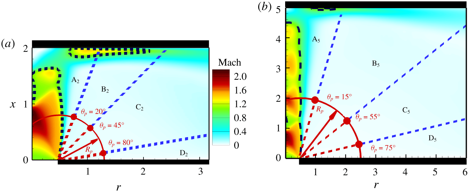
In order to facilitate the discussion, the contour maps of the ensemble-averaged local Mach number defined as the ensemble-averaged local velocity normalised by the ensemble-averaged local speed of sound ( $\sqrt{\unicode[STIX]{x1D6FE}P/\unicode[STIX]{x1D70C}}$) are presented in figure 9. In this figure, the dashed black line shows the sonic line. The regions A to D are marked based on the significant variations in the transfer function as the angular location of the acoustic impulse is varied to facilitate the discussion.
Colourmaps of local Mach number for the nozzle-to-wall distances of (a)  $2d$ and (b)
 $5d$. (Dashed black iso-lines are local Mach number of unity; solid red circle shows the location of the impulse in the impulse simulations with critical angles from the centreline for each case being marked.)

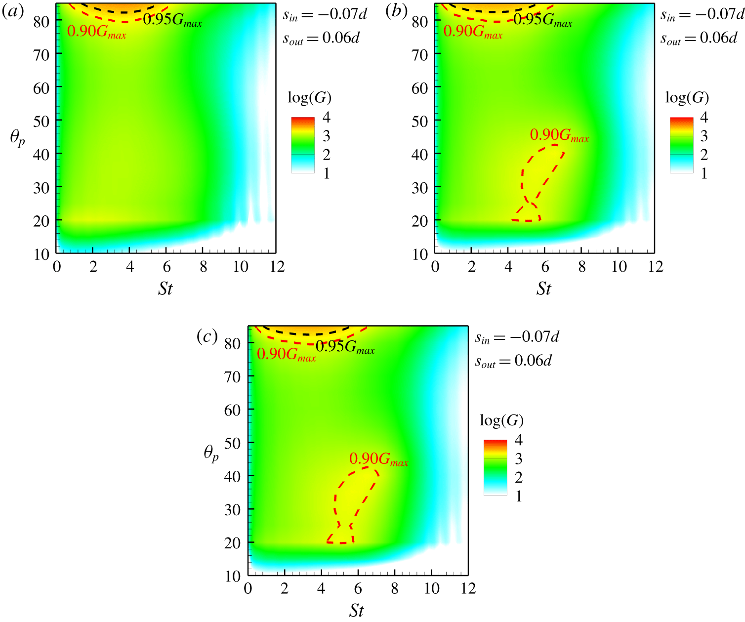
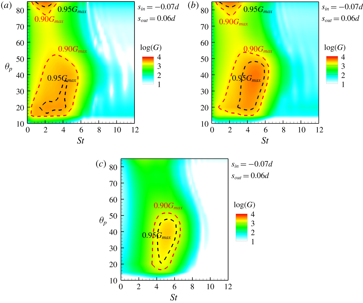
The transfer function quantifying the receptivity is obtained using the method described in § 2. The impulse excites a wide range of frequencies, thus providing the spectrum of the transfer function. The transfer functions,  $G$, for the nozzle-to-wall distances of
 $2d$ and
 $5d$ are presented in figures 10 and 11 for azimuthal mode numbers of
 $m=0$,
 $m=1$ and
 $m=2$. The red and black dashed lines indicate 90 % and 95 % of the maximum value of the transfer function, respectively. The contour level is logarithmic to ensure that the changes in
 $G$ are visible. This analysis shows that the impulses in the vicinity of the impingement wall have the highest amplification in both nozzle-to-wall distance cases. The main findings are summarised as follows.
Contour of the logarithm of the transfer function,  $G$, for the nozzle-to-wall distance of
 $2d$ for azimuthal mode numbers (a)
 $m=0$, (b)
 $m=1$ and (c)
 $m=2$ (90 % and 95 % of the maximum value of the transfer function are marked with red and black dashed lines, respectively).

Contour of the logarithm of the transfer function,  $G$, for the nozzle-to-wall distance of
 $5d$ for azimuthal mode numbers (a)
 $m=0$, (b)
 $m=1$ and (c)
 $m=2$ (90 % and 95 % of the maximum value of the transfer function are marked with red and black dashed lines, respectively).

(i) Nozzle-to-wall distance of 2d (figures 9a and 10):
(a) The transfer function has its minimum value for the acoustic impulse located at an angular position less than
 $20^{\circ }$ (region labelled as $\text{A}_{2}$ in figure 9a). This is due to the blockage of the acoustic waves by the expanded shear layer of the jet. This is clear as the sonic line bulges out at $x\approx 0.5$, resulting in acoustic waves being blocked from directly reaching the nozzle lip. This is consistent with the experimental observation of Raman (Reference Raman1997).
(b) A pressure impulse in the region
$\text{B}_{2}$ ($20^{\circ }<\unicode[STIX]{x1D703}_{p}<45^{\circ }$) travels towards the nozzle and reaches the nozzle lip directly. The transfer function shows amplification of an input signal over a broad range of frequencies with a maximum transfer function at a Strouhal number of 4.0 which is insensitive to the angular position of the impulse for the axisymmetric azimuthal mode. In contrast, for higher azimuthal mode numbers, the maximum transfer function shifts towards a higher Strouhal number as the angular position of the acoustic impulse increases.(c) A low amplification of the input signal occurs if the impulse is located between angles of
$45^{\circ }$ and $80^{\circ }$ (marked as $\text{C}_{2}$). This is consistent among all the azimuthal mode numbers.(d) The maximum amplification of an input signal occurs if the pressure impulse is located near the nozzle lip, i.e. the angle from the jet axis is more than
$80^{\circ }$. This region is labelled by $\text{D}_{2}$. The input signal is amplified over a wide range of frequencies with Strouhal numbers in the range of 0.5–6.2. The peak of the amplification occurs at a Strouhal number of 3.0. This broad spectrum is due to the nozzle lip (Raman Reference Raman1997; Rogler & Reshotko Reference Rogler and Reshotko1975). The optimal amplification of the impulse in the vicinity of the nozzle lip is independent of the azimuthal mode number. A similar behaviour is observed for all three azimuthal mode numbers of 0, 1 and 2.
(ii) Nozzle-to-wall distance of 5d (figures 9b and 11):
(a) An input signal generated by a pressure impulse located in the region
$\text{A}_{5}$ (i.e. for angles between $10^{\circ }$ and $15^{\circ }$) is slightly amplified by the nozzle lip and the transfer function has a small value. This is similar to the case of the smaller nozzle-to-wall distance, and the same hypothesis applies – the expanded shear layer blocks the acoustic waves from direct view. However, as the nozzle-to-wall distance is greater compared to the previous case, the angular limit is slightly narrower.(b) For the pressure impulse located in the region
$\text{B}_{5}$ ($15^{\circ }<\unicode[STIX]{x1D703}_{p}<55^{\circ }$), the transfer function shows the maximum amplification of the input signal. All three azimuthal mode numbers show a high amplification of an incoming signal with the azimuthal mode number of 2 (i.e. helical mode) being dominant. A high amplification occurs over a wide range of frequencies (i.e. a broad range of Strouhal numbers) for the first two azimuthal mode numbers, while occurring over a narrower frequency band for the azimuthal mode number of 2. The maximum value of the transfer function depends on the angular position of the impulse in this region. As the location of the pressure impulse moves towards the infinite-lipped nozzle wall, the Strouhal number of the maximum transfer function increases for all three azimuthal mode numbers.(c) The receptivity of the nozzle lip to acoustic waves created by a pressure impulse located in the region
$\text{C}_{5}$ is limited to the low-frequency band. The peak of the transfer function is shifted to the low-frequency band as the impulse location moves towards the infinite-lipped nozzle wall for the azimuthal mode numbers of 0 and 1, while it is independent of the impulse location for the azimuthal mode number of 2. The amplification of an incoming signal occurs in a slightly narrower frequency range compared to the incoming signal generated by an impulse located in the region $\text{B}_{5}$.(d) The second maximum of the transfer function occurs when the pressure impulse is located near to the infinite-lipped nozzle in the region
$\text{D}_{5}$ and only exists for the axisymmetric and helical modes, i.e. $m=0$ and $1$. In contrast to $h=2d$, high amplification is observed in narrow-band low frequencies, i.e. low Strouhal numbers.


The observed differences in the receptivity for the  $h=2d$ and
 $h=5d$ cases provided quantitatively via the computed transfer functions are a consequence of the base ingredient to the linearised Navier–Stokes solutions, namely the mean flow field (Beneddine et al. Reference Beneddine, Sipp, Arnault, Dandois and Lesshafft2016).
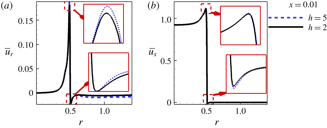
Figures 12(a) and 12(b) show the profiles of the ensemble-averaged radial and streamwise velocities at  $x=0.01$, respectively. There are clear differences in the ensemble-averaged radial velocity, indicating slightly higher entrainment in the case of
 $h=2d$. The ensemble-averaged streamwise velocity has a negative value outside of the jet’s periphery where this negative value is slightly higher for the case of
 $h=5d$.
The profiles of the ensemble-averaged (a) radial and (b) streamwise velocities at  $x=0.01$ for both nozzle-to-wall distances of
 $2d$ (solid black line) and
 $5d$ (dashed blue line).

5 Conclusion
The receptivity at the nozzle lip of under-expanded supersonic impinging jets has been investigated. A transfer function is defined to quantify the receptivity as the ratio of the total energy of the input irrotational acoustic signal to the output vortical fluid dynamic signal at the nozzle lip. The linearised three-dimensional Navier–Stokes equations are solved using an acoustic impulse to simulate a sound source. The acoustic pulse is located at a fixed radius and variable angle from the jet axis. This allows the investigation of the sensitivity of the transfer function to the acoustic impulse location and the azimuthal mode number. It has been demonstrated that the nozzle lip has the highest transfer function when the acoustic field originates from an acoustic source located close to the wall which forms the infinite-lipped nozzle. This is consistent for the first two azimuthal mode numbers for both nozzle-to-wall distances except for acoustic disturbances which have an azimuthal mode number of 2 when  $h=5d$. In this case, the results indicate that there is a second maximum in the transfer function, which occurs when the acoustic field originates from an acoustic impulse located in the region halfway between the infinite-lipped nozzle surface and the shear layer, i.e. for angles between
 $15^{\circ }$ and
 $50^{\circ }$.
The most striking conclusion to emerge from this analysis is the suggestions for effective control of instabilities in under-expanded supersonic impinging jets and, hence, the elimination or minimisation of self-sustained oscillations in under-expanded supersonic impinging jets. The two nozzle-to-wall distances of  $2d$ and
 $5d$ of this study have demonstrated the sensitivity of the receptivity to the angular location of acoustic sources. For under-expanded supersonic impinging jets with a nozzle-to-wall distance of
 $2d$, the receptivity at the nozzle lip is dominated primarily by acoustic sources that are located at angular positions greater than
 $80^{\circ }$ from the jet centreline. Whereas for
 $h=5d$, there are two angular locations where the acoustic waves originating from an acoustic impulse significantly influence the receptivity at the nozzle lip. One is at angular locations greater than
 $80^{\circ }$ from the jet centreline, which is similar to the case of nozzle-to-wall distance of
 $2d$, while the other is an angular region bounded between
 $15^{\circ }$ and
 $55^{\circ }$ from the jet centreline. This behaviour indicates the dynamic nature of the instabilities, highlighting the practical difficulties that arise in using passive control strategies for effective control in industrial applications where the nozzle-to-wall distance changes rapidly. However, when the nozzle-to-wall distance is fixed, a passive control strategy to control the instabilities would be the elimination of acoustic waves which are reflected by near surfaces including the infinite-lipped nozzle surface. This can be achieved by a properly designed sound absorber attached to the reflective surfaces.
Acknowledgements
This work was supported by the Australian Research Council. The research benefited from computational resources provided through the National Computational Merit Allocation Scheme, supported by the Australian Government. The computational facilities supporting this project included the Australian NCI Facility, the partner share of the NCI facility provided by Monash University through an ARC LIEF grant, Pawsey Supercomputing Centre and the Multi-modal Australian ScienceS Imaging and Visualisation Environment (MASSIVE).
Supplementary movies
Supplementary movies are available at https://doi.org/10.1017/jfm.2020.63.