Introduction
Passive radar is a radar system that employs third-party illuminators to achieve a range of objectives, including target detection, direction-of-arrival estimation, imaging, and crowd-monitoring [Reference Zhang, Shi, Yan and Gong1–Reference Storrer, Yildirim, Willame, Pocoma Copa, Cakoni, Pollin, Louveaux, De Doncker and Horlin4]. It utilizes existing communication, radio, and television signals as illuminators of opportunity (IOs) instead of dedicated transmitters, thereby reducing costs and avoiding spectrum interference. In the present era, the majority of wireless communication systems, including Digital Video Broadcasting on Terrestrial, Digital Television Terrestrial Multimedia Broadcasting, Digital Radio Mondiale (DRM), and Wi-Fi, employ orthogonal frequency division multiplexing (OFDM) signals as communication signals [Reference Hu, Yi, Wan, Cheng, Hu and Hao5–Reference Li, Bocus, Tang, Piechocki, Woodbridge and Chetty8]. Consequently, OFDM-based passive radar systems have become a research focus.
Differing from traditional radar systems, OFDM-based passive radar systems typically extract the direct-path signal as a reference. This enables generation of the range-Doppler (RD) spectrum through two-dimensional matched filtering of reference and surveillance signals. Target detection and parameter estimation are subsequently performed on the RD spectrum using statistical methods. However, passive radar faces the challenge of strong direct-path interference and multipath clutter in the surveillance channel, which can mask weak targets in the RD map. Therefore, clutter suppression is usually necessary to eliminate the masking effect on the targets. The common processing methods incorporate adaptive clutter suppression in the spatial domain, temporal domain, or some joint domain and Matched Filter (MF) processing [Reference Sun, Shan, Feng, He, Bai and Zhang9–Reference Colone, O’Hagan, Lombardo and Baker12]. However, these techniques generally succeed in eliminating the low-Doppler portion of the surveillance signal but simultaneously ignore targets at low Doppler frequencies. In addition, the sidelobes generated by strong targets introduce spurious values in their adjoining Doppler cells, which leads to inaccurate estimates of the positions and amplitudes of weaker targets [Reference Feng, Friedt, Cherniak and Sato13].
In recent years, sparse representation theory has been widely studied to address issues related to sidelobes and resolution in passive radar signal processing [Reference Zheng and Wang14–Reference Zhao, Gong, Zhou and Cao18]. It exploits the prior knowledge of sparsity inherent in radar scenes to develop the sparse recovery (SR) model and optimally solves the SR model by incorporating sparse constraint terms to obtain sparse coefficient vectors corresponding to the complex amplitudes of the potential target signal and clutter. After generating a sparse coefficient RD spectrum, a sparse vector with the non-zero values can be directly the detections or a Constant False Alarm Rate-like processor can be designed to perform target detection [Reference Anitori, Maleki, Otten, Baraniuk and Hoogeboom19]. In fact, it falls under the category of the convex optimization problem, termed the least absolute shrinkage and selection operator (LASSO). It is theoretically analyzed and experimentally verified that the SR-based algorithms can achieve better resolution and estimation performance than the conventional clutter suppression algorithms and MF processing algorithms for the estimation of multiple echoes from multipath, clutter, and targets [Reference Feng, Friedt, Cherniak and Sato13].
Nevertheless, the efficient or accurate algorithms of the SR or convex optimization solving are also key points to consider in applications. Three main classes of SR algorithms have been widely studied and applied to the classical SR problem, including orthogonal matching pursuit [Reference Wen, Zhou, Li and Tang20], sparse Bayesian learning (SBL) [Reference Khanna and Murthy21], and iterative optimization algorithms that use  $\ell _{1}$-norm sparse regularization, such as the iterative soft thresholding algorithm [Reference Kamilov and Mansour22], the approximate message passing [Reference Borgerding, Schniter and Rangan23], and the alternating direction method of multipliers (ADMM) [Reference Shentu, Lai, Wang and Cao24], which use shrinkage thresholding function to solve the LASSO problem. In general, iterative optimization algorithms not only ensure that a globally optimal solution is obtained but are also more computationally efficient than SBL when dealing with large-scale data [Reference Arjoune, Kaabouch, El Ghazi and Tamtaoui25]. However, iterative optimization algorithms have three main limitations. Initially, the search process for SR solutions often requires hundreds of iterations. Secondly, parameter selection requires human intervention and different parameter choices may affect the convergence speed and recovery results. Finally, these algorithms lack generality and may require parameter readjustment when the input data undergoes alteration.
To address these challenges, deep learning methodologies have been extensively investigated, with model-driven deep unfolding networks (DUNs) [Reference Monga, Li and Eldar26–Reference Shlezinger, Whang, Eldar and Dimakis28] emerging as a significant approach that maps iterative optimization algorithms to DNNs by designing layers as iterations and converting algorithm parameters into learnable weights for accelerated convergence. While DUNs demonstrate superior performance in imaging radars (e.g., SAR/ISAR) [Reference Yang, Sun, Li and Xu29–Reference Wang, Wei, Liang, Liu, Shi and Zhang34], their application to passive radar is hindered by time-varying SR models due to uncontrollable IOs; this limitation is resolved by our proposed time-invariant SR model for OFDM passive radar [Reference Zhao, Cao, Wang and Zhou35], enabling the target detection framework in this paper. Furthermore, conventional DUNs rely on sparsity priors that lack discriminative power for complex signals [Reference Hieu, Hoang, Nguyen and Alsheikh36], whereas generative priors (e.g., GANs [Reference Creswell, White, Dumoulin, Arulkumaran, Sengupta and Bharath37–Reference Liu, Wang, Yang and Li39]) model authentic signal distributions to outperform sparsity-based methods [Reference Hand and Voroninski40] – though their representational capabilities confine solutions to predefined ranges; consequently, we investigate both DUN solutions and generative-prior-enhanced frameworks for OFDM passive radar detection.
Overall, in this paper, two SR networks are investigated for target detection in OFDM-based passive radar. First, by integrating sparsity prior information into the SR task via regularization, and extending the iterative equations solved by the ADMM algorithm into layer-fixed DNNs with trainable parameters, an SR model-driven deep learning framework called SR-ADMM-Net is proposed, aiming to find the optimal parameters of the ADMM automatically and further accelerate the convergence process through the high fitting ability of DNNs. Second, based on the fact that more complex nonlinear structures can be revealed by utilizing prior distributions learned from generative models as constraints, another deep-learning approach based on the generative model least squares generative adversarial network (LSGAN), called SR-LSGAN, is proposed to achieve better SR performance. Different from conventional techniques reliant on a generative prior, this proposed approach calibrates the parameters of a pre-trained LSGAN through a hybrid approach integrating gradient descent and internal learning, enabling the pre-trained LSGAN to be adaptive and explore solutions beyond its original range. Furthermore, practical target detection applications of passive radar may encounter scenarios where the target intensity is much lower than clutter or entirely obscured. To further improve the detection capability of weak targets, a step-by-step estimation approach is proposed to facilitate weak target detection. In particular, the complex amplitudes of clutter, as firstly estimated from the sparse coefficients vectors generated by the network, are employed to reconstruct and mitigate clutter from the surveillance signal, and then the resultant clutter-free surveillance signal is utilized for MF with the reference signal, thereby achieving the detection of weak targets.
The remainder of this paper proceeds as follows. Section “Background” introduces the time-invariant SR model for OFDM-based passive radars. Section “SR-ADMM-Net” describes the flow of the ADMM algorithm and SR-ADMM-Net details. The proposed SR-LSGAN algorithm is introduced in Section “SR-LSGAN”. Section “Measured Results” demonstrates the effectiveness of the two proposed network-based methods through numerical simulations, including the step-by-step estimation approach for weak target detection. Section “Measured Results” presents the measured experimental results. Finally, Section “Conclusion” concludes and discusses future perspectives.
Background
Signal model
A typical OFDM-based passive radar system comprises two signal channels: reference and surveillance channels. In the reference channel, the received signal may exhibit interference, such as multipath signals and noise, in addition to the direct-path signal. Generally, the direct-path signal can be reconstructed and used as the pure reference signal [Reference Poullin41, Reference Wojaczek, Cristallini, Schell, O’Hagan and Summers42].
 \begin{equation}
{x}_{\text{ref}}[n]=d[n]
\end{equation}
where  $d[n]$ is the complex envelope of the direct-path signal, which is composed of OFDM symbols. A complete OFDM symbol usually consists of the useful part and the cyclic prefix (CP). Following the definition of CP-OFDM waveforms, the time-domain discrete form of the transmitted CP-OFDM signal can be expressed as follows:
 \begin{equation}
d[n]=\sum\limits_{l=0}^{L-1}{{{d}_{l}}[n-l{{N}_{\text{e}}}]}
\end{equation}
where  ${{N}_{\text{e}}}={{N}_{\text{u}}}+{{N}_{\text{cp}}}$ denotes the number of samples of a complete CP-OFDM symbol, consisting of the number of CP sample size
 ${{N}_{\text{cp}}}$ and the number of subcarriers
 ${{N}_{\text{u}}}$. The parameter
 $L$ is the total number of symbols, and
 ${{d}_{l}}(n)$ denotes the
 $l$th OFDM symbol with
 \begin{equation}
{{d}_{l}}[n]=\sum\limits_{k=0}^{{{N}_{\text{u}}}-1}{{{C}_{l,k}}{{e}^{j\frac{2\pi }{{{N}_{\text{u}}}}kn}}},n\in [-{{N}_{\text{cp}}},{{N}_{\text{u}}}]
\end{equation}
where  $C{}_{l,k}$ represents the complex modulation data for the
 $k$th subcarrier in the
 $l$th symbol.
The signal received from the surveillance channel generally contains direct-path interference, multipath signals, target echoes, and noise. Accordingly, the discrete form of the surveillance signal can be modeled as:
 \begin{equation}
\begin{aligned}
{x}_{\text{surv}}[n] = &\sum\limits_{i=0}^{{{N}_{c}}} {{c}_{i}}d[n-n_{i}^{c}] \\
&+ \sum\limits_{q=1}^{{{N}_{t}}} {{\alpha }_{q}}d[n-{{n}_{q}}]{{e}^{j2\pi {{f}_{q}}n}} \\
&+ {{n}_{\text{surv}}[n]}, \quad \forall n=0,1,...,{{N}_{\operatorname{int}}}-1
\end{aligned}
\end{equation}
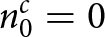
where  ${{c}_{0}}$ and
 $n_{0}^{c}=0$ denote the corresponding complex amplitude and discrete delay of the direct-path signal. Moreover,
 ${{c}_{i}}$ and
 $n_{i}^{c}$ are the complex amplitude and the discrete delay of the
 $i$th multipath echoes, respectively.
 ${{\alpha }_{q}}$,
 ${{n}_{q}}$, and
 ${{f}_{q}}$ are the complex amplitude, the discrete delay, and the Doppler frequency of the
 $q$th target echo, respectively.
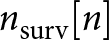 ${{n}_{\text{surv}}}[n]$ is the Gaussian white noise in the surveillance channel, and
 ${{N}_{\text{int}}}$ is the number of all the discrete samples.
SR model and optimization problem for target detection
The sparsity of the echo components in passive radar can be shown in (4), which is the basis of the sparse modeling of the received data and target detection. However, it’s also obvious that the received data are dependent on non-cooperative transmit waveform, resulting in many SR models and their dictionary matrices being time-varying with the transmit waveform or direct-path signal  $d[n]$. A challenge of using a deep-learning network in solving the optimization problem of time-varying SR models is that pre-training a deep-learning network on a dataset generated from one particular transmit waveform may yield non-desirable performance when tested on a different transmit waveform. Specifically, the dictionary matrix of tested data pairs usually does not match the pre-training dictionary matrix due to its varying nature with the transmit waveforms and this mismatch has the potential to significantly impact the performance of the network and the rate of convergence. To address this challenge, our proposed time-invariant SR model and the associated optimization problem will be discussed next.
The idea of the time-invariant SR model is to use only the deterministically known pilots to make the dictionary matrix fixed [Reference Zhao, Cao, Wang and Zhou35]. It first performs discrete Fourier transform (DFT) on each OFDM symbol of the time-domain surveillance signal, next extracts the observation data at the pilot positions, and then performs inverse discrete Fourier transform (IDFT) on it to obtain the new time-domain surveillance signal; similarly, the transmitted data containing only the pilots are performed IDFT to the time domain as the new reference signal; and finally RD-domain data after MF are used to construct the SR model.
First, the time-domain surveillance signal, upon division into OFDM symbols, can be represented as:
 \begin{equation}
{{x}_{\text{surv}}}[n]=\sum\limits_{l}^{L-1}{x_{\text{surv}}^{l}[n-l{{N}_{\text{e}}}]+{{n}_{\text{surv}}}[n]}
\end{equation}
where  $x_{\text{surv}}^{l}[n]=\sum\limits_{k=0}^{{{N}_{\text{u}}}-1}{{{R}_{l,k}}{{e}^{j\frac{2\pi }{{{N}_{\text{u}}}}kn}},n\in [-{{N}_{\text{cp}}},{{N}_{\text{u}}}]}$,
 ${{R}_{l,k}}$ represents the complex modulation data on the
 $k$th subcarrier in the
 $l$th symbol of the surveillance signal. Consequently, after the CPs within each symbol are removed, and the useful parts are subjected to DFT, the surveillance signal in the subcarrier domain can be represented as follows:
 \begin{equation}
{{\mathbf{x}}_{\text{surv}\_\text{sc}}}={{[\mathbf{x}_{\text{surv}\_\text{sc}}^{0},...,\mathbf{x}_{\text{surv}\_\text{sc}}^{l},...,\mathbf{x}_{\text{surv}\_\text{sc}}^{L-1}]}^{\text{T}}}
\end{equation}
where  ${{(\cdot )}^{\text{T}}}$ denotes the transpose, and
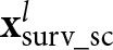 $\mathbf{x}_{\text{surv}\_\text{sc}}^{l}$ represent the
 $l$th symbol of the surveillance signal in the subcarrier domain, respectively, which can be expressed:
 \begin{equation}
\mathbf{x}_{\text{surv}\_\text{sc}}^{l}=\text{DFT}[x_{\text{surv}}^{l}[n]]={{[{{R}_{l,0}},{{R}_{l,1}},...,{{R}_{l,k}},...,{{R}_{l,{{N}_{\text{u}}}-1}}]}^{\text{T}}}
\end{equation}
It is known that pilots are typically incorporated into OFDM waveforms for channel estimation. This allows for establishing a time-invariant SR model without needing reference signals for OFDM passive radar [Reference Zhao, Cao, Wang and Zhou35]. By keeping the complex modulation data at the pilot positions in (7) and setting the complex modulation data at the remaining positions to zero, the complex modulation data at all pilot positions in the surveillance signal within each symbol can be obtained:
 \begin{equation}
\mathbf{x}_{\text{surv}\_\text{p}}^{l}={{[{{M}_{l,0}},...,{{M}_{l,k}},...,{{M}_{l,{{N}_{\text{u}}}-1}}]}^{\text{T}}}
\end{equation}
where
 \begin{equation*}{{M}_{l,k}}=\left\{\begin{array}{l@{\quad}l}
{{R}_{l,k}}, \,k=p \\
0, \,\text{otherwise.}\end{array}\right.
\end{equation*}
 $p$ represents the index of the pilot within each symbol. Following the application of IDFT to the data in (8), the CPs are then incorporated into each symbol to obtain the new surveillance signal
 $z[n]$. Similarly, the corresponding new reference signal
 $v[n]$ can be generated. It should be noted that since the reference signal generated in this paper only requires pilot information and the payload data symbols are set to zero, there is no need at all to perform demodulation/remodulation processing on the reference channel signal. In fact, there is no need to set up the reference channel anymore. According to (4), the relationship between
 $z[n]$ and
 $v[n]$ can be ascertained:
 \begin{equation}
z[n]=\sum\limits_{i=0}^{{{N}_{c}}}{{{c}_{i}}v(n-n_{i}^{c})+\sum\limits_{q=1}^{{{N}_{t}}}{{{\alpha }_{q}}v(n-{{n}_{q}})}{{e}^{j2\pi {{f}_{q}}n}}+\sigma [n]}
\end{equation}
where  $\sigma [n]$ is the error term. By computing the cross-ambiguity function (CAF) between the new reference and surveillance signals, it becomes feasible to estimate the target information.
 \begin{equation}
\chi [\tau ,f]=\sum\limits_{n=0}^{{{N}_{\operatorname{int}}}-1}{z[n]{{v}^{*}}[n-\tau ]}{{e}^{-j2\pi fn/{{f}_{s}}}}
\end{equation}
where  $\tau$ and
 $f$ are the discrete delay and Doppler frequency of the target echo, respectively,
 ${{f}_{s}}$ is the sampling frequency, and
 $(*)$ stands for the conjugate. Substituting (9) into (10) yields:
 \begin{equation}
\chi [\tau ,f]=\sum\limits_{d=1}^{{{N}_{d}}}{{{\beta }_{d}}{{\chi }_{d}}[{{\tau }_{d}},{{f}_{d}}]}
\end{equation}
where  ${{N}_{d}}={{N}_{c}}+{{N}_{t}}+1$ denotes the sum of path numbers of clutter and target echoes.
 ${{\beta }_{d}}\in [{{c}_{0}},...,{{c}_{{{N}_{c}}}},{{\alpha }_{1}},...,{{\alpha }_{{{N}_{t}}}}]$ denotes the vector of complex amplitudes of clutter and target echoes as denoted in (4). Finally, the CAF of the clutter or target echoes with discrete delay
 ${{\tau }_{d}}$ and Doppler frequency
 ${{f}_{d}}$ can be represented as follows:
 \begin{equation}
{{\chi }_{d}}[\tau ,f]=\sum\limits_{n=0}^{{{N}_{\operatorname{int}}}-1}{v[n-{{\tau }_{d}}]{{e}^{j2\pi n{{f}_{d}}}}{{v}^{*}}[n-\tau ]{{e}^{-j2\pi fn/{{f}_{s}}}}}
\end{equation}
Assuming that the time delay and Doppler frequency values do not exceed  $\tau_{\max}$ and
 $f_{\max}$, respectively, the time delay range
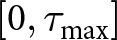 $[0, \tau_{\max}]$ is evenly divided into
 $L_d$ grids, with each grid point corresponding to a time delay value
 $\tau_i$,
 $i=1,\ldots,L_d$. Simultaneously, the Doppler frequency range
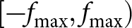 $[-f_{\max}, f_{\max})$ is evenly divided into
 $L_f$ grids, with each grid point corresponding to a Doppler frequency value
 $f_j$,
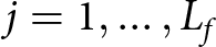 $j=1,\ldots,L_f$. Then, the atom in the
 $((j-1)L_d + i)$-th column of the dictionary matrix
 $\boldsymbol{\Psi}$ can be expressed as follows:
 \begin{equation}
\boldsymbol{\psi}_{(j-1)L_d + i} = \sum_{n=0}^{N_{\text{int}}-1} v[n - \tau_i] \, e^{j2\pi n f_j } \, v^*[n - \tau] \, e^{-j2\pi f n / f_s}
\end{equation}
It is evident that  $\boldsymbol{\Psi}\in \mathbb{C}^{N_{\text{int}}\times J}$ is time-invariant, as it only depends on the new reference signal derived from the fixed pilot information and its dimension
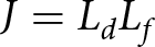 $J = L_d L_f$ is only related to the delay-Doppler grids. Correspondingly, the RD estimation problem for target detection becomes a SR problem as follows:
 \begin{equation}
\mathbf{Y} = \boldsymbol{\Psi} \mathbf{x} + \mathbf{e}
\end{equation}
where  $\mathbf{Y}$ represents the CAF between the new reference signal and the new surveillance signal,
 $\mathbf{x}$ is a vectorized RD map and also a sparse coefficient vector containing the complex amplitudes of the target and clutter, and
 $\mathbf{e}$ is the vectorized error. Consequently, it is sufficient to estimate the non-zero component of
 $\mathbf{x}$ to obtain the target information. By imposing a sparsity constraint on
 $\mathbf{x}$ in (14), it can be transformed into the following optimization problem:
 \begin{equation}
\underset{\mathbf{x}}{\mathop{\min }}\,||\mathbf{x}|{{|}_{0}}\,\text{s}\text{.t}\text{. }||\mathbf{Y}-\boldsymbol{\Psi} \mathbf{x}||_{2}^{2}\le \varepsilon
\end{equation}
where  $||\cdot |{{|}_{b}}$ denotes the matrix
 $\ell _{b}$-norm. Since the objective function
 $||\cdot |{{|}_{0}}$ is nonconvex, the optimization problem in (15) is NP-hard, where NP stands for nondeterministic polynomial time, and thus is practically infeasible to solve optimally. One way to solve such a problem is to approximate the solution by replacing the
 $\ell _{0}$-norm with the
 $\ell _{1}$-norm. Thus, the above optimization problem is transformed into the following LASSO problem:
 \begin{equation}
\underset{\mathbf{x}}{\mathop{\min }}\,\frac{1}{2}||\mathbf{Y}-\boldsymbol{\Psi} \mathbf{x}||_{2}^{2}+\lambda ||\mathbf{x}|{{|}_{1}}
\end{equation}
where 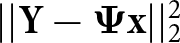 $||\mathbf{Y}-\boldsymbol{\Psi} \mathbf{x}||_{2}^{2}$ is a linear equation that controls the fidelity and
 $\lambda $ is a regularization factor controlling the trade-off between fidelity and sparsity of
 $\mathbf{x}$.
The ADMM algorithm is an iterative optimization algorithm that is particularly effective for addressing large-scale optimization challenges, including those associated with the LASSO problem. The fundamental idea is to decompose the initial global optimization problem into a sequence of more tractable local subproblems, which usually yield closed-form solutions that can guarantee convergence to a point proximate to the optimal solution. However, the ADMM algorithm is sensitive to parameter selection, and improper parameter selection may affect the convergence speed of the algorithm and the quality of the final solution. Additionally, the computational burden associated with each iteration is considerable. As a result, researchers have turned their attention to deep learning networks.
Method
SR-ADMM-Net
The DUN represents a type of network that combines iterative optimization algorithms with deep learning architectures. The fundamental concept involves unfolding and integrating the iterative optimization algorithms into the DNN framework, capitalizing on the intrinsic parallelism of the DNN to automatically learn the optimal algorithm parameters and expedite the convergence process. This section initially derives the iterative equations pertinent to ADMM solving (16), followed by a description of the design of the SR-ADMM-Net framework.
ADMM solver
By introducing the independent auxiliary variable  $\mathbf{s}$, the optimization problem in (16) can be equated to the following constrained problem:
 \begin{equation}\begin{array}{ll}
& \underset{\mathbf{x,s}}{\mathop{\min }}\,\frac{1}{2}||\mathbf{Y}-\boldsymbol{\Psi} \mathbf{x}||_{2}^{2}+\lambda ||\mathbf{s}|{{|}_{1}} \\
& \text{s}\text{.t}\text{. }\mathbf{x}-\mathbf{s}=0 \\
\end{array}\end{equation}
Its augmented Lagrangian function is:
 \begin{equation}
\begin{array}{ll}
{{L}_{\rho }}(\mathbf{x},\mathbf{s}\text{,}\mathbf{u}) & =\frac{1}{2}||\mathbf{Y}-\boldsymbol{\Psi} \mathbf{x}||_{2}^{2}+\lambda ||\mathbf{s}|{{|}_{1}}+ \\
&\frac{\rho }{2}||\mathbf{x-s+u}||_{2}^{2}-\frac{\rho }{2}||\mathbf{u}||_{2}^{2}
\end{array}
\end{equation}
where  $\mathbf{u}$ is the Lagrange multiplier and
 $\rho $ is a penalty parameter. According to the algorithm definition, the ADMM decomposes (18) into three subproblems to optimize the variables
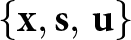 $\left\{\mathbf{x,s,}\left. \mathbf{u} \right\} \right.$ alternately. During the
 $t$th iteration, the iterative equation is as follows:
1)  $\mathbf{x}$-Update: Fix
 $\mathbf{s}$ and
 $\mathbf{u}$ to update
 $\mathbf{x}$; the objective function concerning the variable
 $\mathbf{x}$ can be articulated as follows:
 \begin{equation}
{{\mathbf{x}}^{t}}=\underset{\mathbf{x}}{\mathop{\text{argmin}}}\,\frac{1}{2}||\mathbf{Y}-\boldsymbol{\Psi} \mathbf{x}||_{2}^{2}+\frac{\rho }{2}||\mathbf{x}-{{\mathbf{s}}^{t-1}}+{{\mathbf{u}}^{t-1}}||_{2}^{2}
\end{equation}
Equation (19) is essentially a  $\ell _{2}$-norm regularized least squares problem that can be solved using gradient descent.
2)  $\mathbf{s}$-Update: Fix
 $\mathbf{x}$ and
 $\mathbf{u}$ to update
 $\mathbf{s}$; the objective function concerning the variable
 $\mathbf{s}$ can be articulated as follows:
 \begin{equation}
{{\mathbf{s}}^{t}}=\underset{\mathbf{s}}{\mathop{\text{argmin}}}\,\frac{\rho }{2}||{{\mathbf{x}}^{t}}-\mathbf{s}+{{\mathbf{u}}^{t-1}}||_{2}^{2}+\lambda ||\mathbf{s}|{{|}_{1}}
\end{equation}
Equation (20) involves solving an optimization problem with  ${{\ell }_{1}}$-norm regularization that can be approximated by a soft-thresholding function, which is given as
 \begin{equation}
{{\eta }_{\varsigma }}(\kappa )=\text{sign}(\kappa )\text{max}(0,|\kappa |-\varsigma )
\end{equation}
Note that  $\varsigma $ denotes threshold parameter, and
 \begin{equation}
\text{sign(}\kappa \text{)=}\left\{\begin{aligned}
& \kappa /|\kappa |, \kappa \ne 0 \\
& 0\text{ , }\kappa =0 \\
\end{aligned}
\right.
\end{equation}
3)  $\mathbf{u}$-Update: Fix
 $\mathbf{x}$ and
 $\mathbf{s}$ to update
 $\mathbf{u}$; the objective function concerning the variable
 $\mathbf{u}$ can be articulated as follows:
 \begin{equation}
{{\mathbf{u}}^{t}}={{\mathbf{u}}^{t-1}}+\beta ({{\mathbf{x}}^{t}}-{{\mathbf{s}}^{t}})
\end{equation}
where  $\beta $ is an update rate for the Lagrangian Multiplier.
Namely, the iterative equations for ADMM to solve (17) are
 \begin{equation}
\left\{\begin{aligned}
& {{\mathbf{x}}^{t}}={{({{\boldsymbol{\Psi}}^{\text{T}}}\boldsymbol{\Psi}+\rho \mathbf{I})}^{-1}}({{\boldsymbol{\Psi}}^{\text{T}}}\mathbf{Y}+\rho ({{\mathbf{s}}^{t-1}}-{{\mathbf{u}}^{t-1}})) \\
& {{\mathbf{s}}^{t}}={{\eta }_{\lambda /\rho }}({{\mathbf{x}}^{t}}+{{\mathbf{u}}^{t-1}}) \\
& {{\mathbf{u}}^{t}}={{\mathbf{u}}^{t-1}}+\beta ({{\mathbf{x}}^{t}}-{{\mathbf{s}}^{t}}) \\
\end{aligned}
\right.
\end{equation}
where  $\mathbf{I}$ is an identity matrix, and
 ${{(\cdot )}^{-1}}$ denotes matrix inverse.
As illustrated in (24), the ADMM algorithm necessitates a substantial amount of matrix operations, inevitably resulting in a significant computational burden. Moreover, determining the most suitable values for the parameters  $\rho $,
 $\lambda $, and
 $\beta $ in the ADMM solver poses a considerable challenge. To address these challenges, a DUN SR-ADMM-Net is developed using the iterative equations of the ADMM algorithm, wherein the
 $t$th iteration of the ADMM algorithm corresponds to the
 $t$th layer of the SR-ADMM-Net. In addition, the strong dependence of the ADMM algorithm on manual parameter selection is reduced by converting the parameters
 $\rho $,
 $\lambda $, and
 $\beta $ into a series of learnable parameters, thus improving the generalization capability.
SR-ADMM-Net structure
The network structure of SR-ADMM-Net is illustrated in Figure 1, in which each layer consists of three modules: the reconstruction module  ${{\mathbf{X}}^{(t)}}$, the nonlinear transform module
 ${{\mathbf{S}}^{(t)}}$, and the multiplier update module
 ${{\mathbf{U}}^{(t)}}$. Furthermore, a comprehensive description of the update procedure within SR-ADMM-Net is provided, which encompasses the formulation of the learnable parameters to facilitate rapid convergence.
Data flow graph for SR-ADMM-Net.

Figure 1 Long description
The diagram illustrates the data flow graph for SR-ADMM-Net, consisting of multiple layers labeled as Layer 1 and Layer t. On the left, the input Y is shown entering Layer 1, which contains three modules: the reconstruction module labeled X superscript 0, the nonlinear transform module labeled S superscript 0 and the multiplier update module labeled U superscript 0. Arrows indicate the flow of data between these modules, with X superscript 0 connecting to S superscript 0 and U superscript 0 and S superscript 0 connecting back to X superscript 0. The diagram continues to Layer t, which similarly contains modules labeled X superscript t, S superscript t and U superscript t, with arrows showing the data flow between them. The output of Layer t is labeled as Sparse Coefficient Vectors x, depicted on the right side of the diagram. The connections between layers are indicated by dashed lines, suggesting continuity and progression through the network structure.
Reconstruction Module  ${{\mathbf{X}}^{(t)}}$: This module reconstructs the sparse coefficient vector
 $\mathbf{x}$ according to the reconstruction operation in (24). Given the inputs
 $\mathbf{Y}$,
 $\boldsymbol{\Psi}$, and
 ${{\mathbf{s}}^{(t-1)}}$,
 ${{\mathbf{u}}^{(t-1)}}$ from layer
 $t-1$, the output of this module in layer
 $t$ is defined as:
 \begin{equation}
{{{\tilde{x}}}^{(t)}}={{({{\boldsymbol{\Psi}}^{\text{T}}}\boldsymbol{\Psi}+{{\rho }^{(t)}}\mathbf{I})}^{-1}}({{\boldsymbol{\Psi}}^{\text{T}}}\mathbf{Y}+{{\rho }^{(t)}}({{{\tilde{s}}}^{(t-1)}}-{{{\tilde{u}}}^{(t-1)}}))
\end{equation}
where  ${{\rho }^{(t)}}$ is a learnable parameter that is mainly used to control the rate of convergence. In the first layer,
 ${{{\tilde{s}}}^{(0)}}$ and
 ${{{\tilde{u}}}^{(0)}}$ are initialized to zero so that
 ${{{\tilde{x}}}^{(1)}}={{\boldsymbol{\Psi}}^{\text{T}}}\mathbf{Y}{{({{\boldsymbol{\Psi}}^{\text{T}}}\boldsymbol{\Psi}+{{\rho }^{(1)}}\mathbf{I})}^{-1}}$.
Nonlinear Transform Module  ${{\mathbf{S}}^{(t)}}$: This module uses the soft-thresholding function defined in (21) to update
 $\mathbf{x}$. Given
 ${{\mathbf{u}}^{(t-1)}}$ and
 ${{\mathbf{x}}^{(t)}}$, the output of this module in layer
 $t$ is defined as:
 \begin{equation}
{{{\tilde{s}}}^{(t)}}={{\eta }_{{{\varsigma }^{(t)}}}}({{{\tilde{x}}}^{(t)}}+{{{\tilde{u}}}^{(t-1)}})
\end{equation}
where  ${{\varsigma }^{(t)}}$ stands for threshold, a learnable parameter determining the final convergence accuracy.
Multiplier update Module  ${{\mathbf{U}}^{(t)}}$: Given the inputs
 ${{\mathbf{u}}^{(t-1)}}$,
 ${{\mathbf{x}}^{(t)}}$ and
 ${{\mathbf{s}}^{(t)}}$, the output of this module in layer
 $t$ is defined as:
 \begin{equation}
{{{\tilde{u}}}^{(t)}}={{{\tilde{u}}}^{(t-1)}}+{{\beta }^{(t)}}({{{\tilde{x}}}^{(t)}}-{{{\tilde{s}}}^{(t)}})
\end{equation}
Here,  ${{\beta }^{(t)}}$ is a learnable parameter that controls the step size of the gradient update.
Network Parameters: In the SR-ADMM-Net framework, the learnable parameters include the step size  ${{\rho }^{(t)}}$ in the reconstruction module, the shrinkage threshold
 ${{\varsigma }^{(t)}}$ in the nonlinear transformation module, and the parameter
 ${{\beta }^{(t)}}$ in the multiplier update module. That is, the set of learned parameters is
 $\Theta =\left\{{{\rho }^{(1)}},{{\varsigma }^{(1)}},\left. {{\beta }^{(1)}},...,{{\rho }^{(t)}},{{\varsigma }^{(t)}},{{\beta }^{(t)}} \right\} \right.$.
Loss function
Since an end-to-end manner is used to train the SR-ADMM-Net, the mean square error is chosen as the loss function. Given the training set  ${{\Omega }_{\text{train}}}$, the loss between the network output
 ${{\mathbf{x}}^{\text{output}}}$ and the ground truth
 ${{\mathbf{x}}^{\text{gt}}}$ is defined as:
 \begin{equation}
Loss=\frac{1}{{{\Omega }_{\text{train}}}}\sum\limits_{i=1}^{{{\Omega }_{\text{train}}}}{||{{\mathbf{x}}^{\text{output}}}-{{\mathbf{x}}^{\text{gt}}}||_{2}^{2}}
\end{equation}
SR-LSGAN
The sparsity-prior-based DUN primarily relies on the judgment capacity of the  ${{\ell }_{1}}$-norm regularizer, i.e., soft-thresholding function. However, the judgment capacity of this function is limited, rendering DUN unable to capture the sparse features of the target and clutter fully. In contrast, a generative-prior-based approach can address this limitation by leveraging prior learned from a vast dataset comprising sparse coefficient vectors. However, its efficacy hinges on the solution space of the pre-trained generator. This section initially delineates the generative model LSGAN and the tenets of the generative prior-based approach. Subsequently, we propose SR-LSGAN, a novel generative-prior-based framework for passive radar target detection. Unlike conventional SR algorithms that rely on explicit
 $\ell_1$-norm sparsity constraints, SR-LSGAN addresses the SR problem formulated in (14) by minimizing
 $\|\mathbf{Y}-\boldsymbol{\Psi}{{G}}(\mathbf{z})\|_{2}^{2}$ with
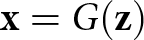 $\mathbf{x} = {{G}}(\mathbf{z})$, where the generator
 ${{G}}$ in the latent space implicitly learns the data distribution of the sparse coefficient samples
 $\mathbf{x}$.
Least squares generative adversarial network
GAN represents an implicit generative model that models the probability density function via a stochastic process directly generating data. A GAN consists of two primary components: the generator  $G$ and the discriminator
 $D$. The generator aims to learn the distribution of real samples and generate fake samples that adhere to this distribution to deceive the discriminator. The discriminator’s role is to differentiate between real samples and those generated by the generator. Specifically, the generator primarily achieves a mapping from a low-dimensional latent space to a high-dimensional sample space:
 $\mathbf{z}\in {{\mathbb{R}}^{a}}\to G(\mathbf{z})\in {{\mathbb{R}}^{b}}, a\ll b$. Thus, given low-dimensional noise vectors
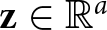 $\mathbf{z}\in {{\mathbb{R}}^{a}}$, the
 $G$ can create samples
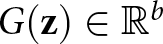 $G(\mathbf{z})\in {{\mathbb{R}}^{b}}$ that are more similar to the real samples
 $\mathbf{x}$. Subsequently, the discriminator evaluates the input samples and outputs a probability value
 $D(\mathbf{x})$ to signify the likelihood that the sample is real. During the training phase, the generative and discriminative networks continuously and alternately update, achieving a dynamic equilibrium. The minimax objective function for the original GAN can be represented as follows:
 \begin{equation}
\begin{aligned}
\underset{G}{\mathop{\min }}\,\underset{D}{\mathop{\max }}\,{{V}_{\text{GAN}}}(D,G) & ={{E}_{\mathbf{x}\sim{{P}_{\text{data}}}(\mathbf{x})}}[\log (D(\mathbf{x}))] \\
& +{{E}_{\mathbf{z}\sim{{P}_{\mathbf{z}}}}}[\log (1-D(G(\mathbf{z}))]
\end{aligned}
\end{equation}
where  $E[\cdot ]$ denotes the average value,
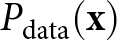 ${{P}_{\text{data}}}(\mathbf{x})$ represents the distribution of real samples, and
 $P(\mathbf{z})$ is the noise vector’s distribution, usually Gaussian.
However, the function in (29) is susceptible to gradient disappearance during training, leading to the model’s collapse. Therefore, to enhance the stability and quality of generation, this paper adopts the LSGAN proposed in [Reference Mao, Li, Xie, Lau, Wang and Smolley43]. LSGAN addresses the limitations of the original GAN by integrating the least squares loss into the adversarial loss function. The loss function of LSGAN is as follows:
 \begin{equation}
\begin{aligned}
\underset{D}{\mathop{\min }}\,{{V}_{\text{LSGAN}}}(D) & =\frac{1}{2}{{E}_{\mathbf{x}\sim{{P}_{\text{data}}}(\mathbf{x})}}[{{(D(\mathbf{x})-\mu_2)}^{2}}] \\
& +\frac{1}{2}{{E}_{\mathbf{z}\sim{{P}_{\mathbf{z}}}(\mathbf{z})}}[{{(D(G(\mathbf{z}))-\mu_1)}^{2}}]
\end{aligned}
\end{equation}
 \begin{equation}
\underset{G}{\mathop{\min }}\,{{V}_{\text{LSGAN}}}(G)=\frac{1}{2}{{E}_{\mathbf{z}\sim{{P}_{\mathbf{z}}}(\mathbf{z})}}{{[D(G(\mathbf{z}))-\mu_3)}^{2}}]
\end{equation}
where  $\mu_1,\mu_2,\mu_3$ is a scalar label that satisfies the equation
 $\mu_2-\mu_3=1,\mu_2-\mu_1=2$ (In this paper
 $\mu_1=-1,\mu_2=1,\mu_3=0$ are used).
Recovering objects using generative priors
The core concept of the generative-prior-based methodology is to leverage the prior knowledge embedded within a pre-trained generative model to address a series of linear inverse problems. Accordingly, for the linear inverse problem delineated in (14), it is sufficient to construct a large training set that encompasses a multitude of sparse coefficient vectors  $\mathbf{x}$ and to train the LSGAN. At this juncture, the pre-trained generator is capable of effectively approximating the high-dimensional prior distributions associated with the set of classes to which
 $\mathbf{x}$ belongs (the training set) and thus can serve as an alternative prior to the sparsity prior in (14). By optimizing noise vector
 $\mathbf{z}$ in the solution space defined by
 $G$, an estimate
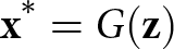 ${{\mathbf{x}}^{*}}=G(\mathbf{z})$ of the true vector
 $\mathbf{x}$ is obtained. Consequently, the resolution of (14) is framed as the minimization of the following loss function:
 \begin{equation}
L(\mathbf{z}) = ||\mathbf{Y}-\boldsymbol{\Psi}G(\mathbf{z})||_{2}^{2}
\end{equation}
This optimization procedure can be viewed as adjusting the noise vector  $\mathbf{z}$ to ensure that the pre-trained generator accurately generates an estimate of the true solution vector
 $\mathbf{x}$. The generator
 $G$ is usually differentiable, allowing for the solution of (32) using the gradient descent. However, the pre-trained generator’s characterization capabilities are limited. When applying gradient descent directly to
 $\mathbf{z}$, the solution space is constrained to
 $G$. Moreover, if initialized improperly, the gradient descent method may converge to a local minimum, often necessitating multiple restarts to achieve optimal performance in practice [Reference Dhar, Grover and Ermon44].
SR-LSGAN algorithm for sparse recovery task
To address the challenge of restricted generator representation capacity, this paper proposes SR-LSGAN, as shown in Figure 2. This methodology enhances generator adaptability during offline training by combining gradient descent with internal learning to fine-tune the pre-trained parameters  $\boldsymbol{\theta}$. Notably, unlike the conventional practice of reconstructing
 $\mathbf{x}$ as
 $G(\mathbf{z})$, our optimization simultaneously adjusts both the noise vector
 $\mathbf{z}$ and generator parameters
 $\boldsymbol{\theta}$ by minimizing the cost function:
 \begin{equation}
L(\mathbf{z},\boldsymbol{\theta }) = ||\mathbf{Y}-\boldsymbol{\Psi}{{G}_{\boldsymbol{\theta }}}(\mathbf{z})||_{2}^{2}
\end{equation}
Overview of the proposed SR-LSGAN using deep generative priors.

Figure 2 Long description
The diagram consists of two main sections separated by a dashed line. On the left, the training process of LSGAN is illustrated. At the top, a discriminator labeled 'D' is shown, which distinguishes between real and fake samples. Real samples are depicted entering the discriminator from the left, while fake samples generated by the generator 'G' enter from the right. Below the generator, Gaussian noise 'Z' is introduced, feeding into the generator to produce fake samples. The generator is labeled 'G subscript theta', indicating it is pre-trained. On the right side, the SR-LSGAN for SR tasks is depicted. At the top, a box labeled 'Gradient Descent' contains two processes: 'Update Z' and 'Update theta', which are part of internal learning. The cost function 'L left parenthesis Z comma theta right parenthesis equals norm Y minus Psi G subscript theta left parenthesis Z right parenthesis norm subscript 2 superscript 2' is shown within this box. Below, Gaussian noise 'Z' is again introduced to the generator 'G subscript theta', producing generated samples 'G left parenthesis Z right parenthesis'. These samples are used to optimize parameters, feeding into the SR task. Sparse coefficient vectors 'X' are shown on the right, calculated as 'X equals G subscript theta left parenthesis Z right parenthesis'. Input 'Y' is depicted entering the gradient descent box from the top left, contributing to the optimization process.
The optimization of (33) can be conducted through backpropagation and the Adam optimizer. This data consistency constraint enhances the reliability of the network-generated data. Given that zero initialization outperforms random initialization,  $\mathbf{z}$ is instantiated to zero in this case. Subsequently, the variables
 $\mathbf{z}$ and
 $\boldsymbol{\theta}$ are concurrently minimized to derive
 $\hat{\mathbf{z}}$ and
 $\hat{\boldsymbol{\theta}}$, and the final estimate
 ${{\mathbf{x}}^{*}}$ is given by:
 \begin{equation}
{\mathbf{x}}^{*}={G}_{\hat{{\theta}}}(\hat{\mathbf{z}})
\end{equation}

Results
Simulation results and analysis
Experiment settings
1) Training Set: In this paper, the transmit OFDM signal is generated based on DRM signals with a bandwidth of 10 KHz, 256 subcarriers, of which only 207 are valid subcarriers and a sampling frequency of 24 KHz. OFDM signals are organized in superframes, each consisting of three transmission frames, in which plum-shaped gain pilots are set for channel estimation. In the surveillance channel, 10–12 scatterers are randomly selected to simulate multipath echoes. The delays and clutter-to-noise ratios (CNRs) of the multipath are randomly determined, with the delay ranging from 0 to 40 sample intervals and the CNRs ranging from 0 to 30 dB. Additionally, the CNR of the direct-path signal is set to 40 dB, and the thermal noise is modeled as complex Gaussian white noise. Additionally, a simulated target echo with random delay and Doppler shift is included in each training set sample. The Doppler shift range of the target is from  $-$10 to 10 Hz, the discrete delay range is from 0 to 20 sample intervals, and the signal-to-noise ratio (SNR) range of the target echo is from
 $-$30 to 10 dB. A total of 480 OFDM symbols are used to generate the training set. The delay range for the dictionary matrix is set to (0:1:40) sample intervals, the Doppler shift range is (
 $-$10:0.2:10) Hz, i.e., the total number of RD grids
 $J$ is 8000, and the total number of samples of sparse coefficient vectors in the training set is 5000.
2) Testing Set: The parameter settings for clutter and target in the testing set are identical to those in the training set, and a total of 2000 samples are generated for the testing set.
3) Preprocess of Complex-Value Data: Since the passive radar data are complex-valued, it is necessary to preprocess the data to enable the general deep neural networks to deal. In this paper, given the complex-valued vectors  $\mathbf{Y}$,
 $\mathbf{x}$ and matrices
 $\boldsymbol{\Psi}$, the matrix-vector multiplication can be decomposed and expressed as:
 \begin{equation}
\left[ \begin{aligned}
& \text{Re(}\mathbf{Y}\text{)} \\
& \text{Im(}\mathbf{Y}\text{)} \\
\end{aligned}
\right]\text{=}\left[ \begin{aligned}
& \text{Re(}\boldsymbol{\Psi}\text{)} \\
& \text{Im(}\boldsymbol{\Psi}\text{)} \\
\end{aligned}
\right.\left. \begin{aligned}
& \text{-Im(}\boldsymbol{\Psi}\text{)} \\
& \text{ Re(}\boldsymbol{\Psi}\text{)} \\
\end{aligned}
\right]\cdot \left[ \begin{aligned}
& \text{Re(}\mathbf{x}\text{)} \\
& \text{Im(}\mathbf{x}\text{)} \\
\end{aligned}
\right]
\end{equation}
where  $\text{Re(}\cdot \text{)}$ and
 $\text{Im(}\cdot \text{)}$ represent the real and imaginary components of the complex-valued data, respectively. By connecting the real and imaginary components of the vectors, reorganizing the matrix as illustrated in (35), and normalizing the data in
 $\mathbf{Y}$ and
 $\boldsymbol{\Psi}$, the complex-valued passive radar data can be handled by SR-ADMM-Net and SR-LSGAN.
4) Network Configuration and Training: In the experiment, the SR-ADMM-Net and LSGAN described in this paper were trained on a Windows 10 operating system using the PyTorch framework. The CPU of the experimental environment is a 7th generation i7-7800X running at 3.50 GHz, and the GPU is an NVIDIA GeForce RTX 2080Ti.
The SR-ADMM-Net was trained using the following hyperparameters: a batch size of 10, a learning rate of 0.001, 20 epochs, 8 network layers, and a dynamic learning rate set to decrease to 0.1 times the original value every 5 epochs to aid convergence. The initial values of the learnable parameters  $\Theta =\left\{{{\rho }^{(0)}},{{\varsigma }^{(0)}},\left. {{\beta }^{(0)}} \right\} \right.$ were set to 0.05, 0.001, 1.
The structure of LSGAN is illustrated in Table 1. The generator and discriminator both comprise fully connected (FC) layers, with the dimensionality of the low-dimensional noise vector  $\mathbf{z}$ set to 100. During the training process, the LSGAN was optimized using the Adam optimizer with the following hyperparameters: the generator’s learning rate was set to 0.0001, the discriminator’s learning rate was set to 0.00005, the batch size was 100 and 400 epochs of training. In algorithm 1, the optimization procedure in (33) was solved by using the Adam optimizer, the number of iterations was set to 5000, and the learning rate of both
 $\mathbf{z}$ and
 $\boldsymbol{\theta }$ was 0.0001.
Detailed specification of LSGAN

Table 1 Long description
The table lists the layer by layer architectures of the LSGAN generator and discriminator, including input sizes, fully connected layer widths, and activation and normalization choices. The generator starts from a noise vector with 100 features and passes through five fully connected layers with widths 256, 512, 1024, 4000, and 8000. After each generator layer, batch normalization is applied and the activation is LeakyReLU. The discriminator takes an input vector with 8000 features and passes through five fully connected layers with widths 4000, 2000, 512, 256, and 1. The discriminator uses LeakyReLU after each layer and does not include batch normalization in this specification. Overall, the generator progressively increases dimensionality to match the 8000 feature output, while the discriminator progressively reduces dimensionality to a single score. The table describes network structure only and does not provide training settings, loss details, or performance results.
5) Step-by-Step Estimation Approach for Weak Target Detection: As shown in Figure 1 and 2, the network output is the sparse coefficient vectors equal to the vectorized RD maps. Consequently, it is possible to directly obtain the coefficient vectors corresponding to the multiple echo components, including clutter and target echoes, following the acquisition of the network output during the testing phase. However, in the field of OFDM passive radar, there are many instances where the target signal is exceedingly weak, with an intensity thousands of times lower than that of the direct-path signal, and it may be totally masked by clutter. In these scenarios, the network may struggle to simultaneously effectively learn the sparse features of the weak target and strong clutter or by one-step processing, which makes the network’s output, vectorized RD maps, produce several false targets caused by noise, potentially resulting in misidentification of the actual target.
Thus, to detect as many weak targets as possible, a step-by-step estimation approach is used as outlined below: after obtaining the sparse coefficient vectors of the network output, the clutter coefficients in the sparse coefficient vectors are extracted to create a clutter-only surveillance signal. It is easy to distinguish the sparse coefficients of clutter because they generally occur near the zero-Doppler frequency of the RD map and usually with stronger intensity. Subsequently, the clutter component is subtracted from the initial surveillance signal by the CLEAN algorithm [Reference Kulpa and Czekala45]. Finally, the resulting signal is match-filtered with the reference signal, thereby enabling the detection of weak targets. The proposed step-by-step estimation approach is illustrated in Figure 3.
Step-by-step estimation approach for weak target detection.

Figure 3 Long description
The diagram is divided into two main sections: Training and Testing. Training section: - Begins with a 'Training set' leading to 'Network output'. - 'Network output' connects to 'Loss', which then leads to 'Sparse coefficient vectors containing clutter and target coefficients'. - A 'Gaussian distribution' feeds into 'LSGAN', which connects to 'Loss'. - 'Loss' leads to 'Generative prior distribution', which connects to 'Distribution of real samples'. Testing section: - Starts with 'Raw surveillance signals' leading to 'SR-ADMM-Net / SR-LSGAN'. - 'SR-ADMM-Net / SR-LSGAN' connects to 'Sparse coefficient vectors containing clutter and target coefficients'. - 'Extracting clutter coefficients' leads to 'Clutter-only surveillance signals'. - 'Clutter-only surveillance signals' connects to 'Reconstruct the clutter component'. - 'Reconstruct the clutter component' leads to 'MF'. - 'MF' connects to 'Obtaining weak target information'.
Results and analysis
1) Simulation 1: Convergence Speed of SR-ADMM-Net vs. ADMM: As stated before, SR-ADMM-Net is proposed to automatically learn the optimal parameters and accelerate the convergence process of ADMM. So, the convergence speeds of SR-ADMM-Net with ADMM will be analyzed in this part. To compare the convergence speed of SR-ADMM-Net with ADMM, the average normalized mean square error (NMSE) calculated on the test set of both methods is utilized for assessment. NMSE in dB scale is defined as:
 \begin{equation}
\text{NMSE}=10{{\log }_{10}}[\frac{1}{{{\Omega }_{\text{test}}}}\sum\limits_{i=1}^{{{\Omega }_{\text{test}}}}{\frac{||{{\mathbf{x}}^{\text{gt}}}-{{\mathbf{x}}^{\text{output}}}||_{2}^{2}}{||{{\mathbf{x}}^{\text{gt}}}||_{2}^{2}}}]
\end{equation}
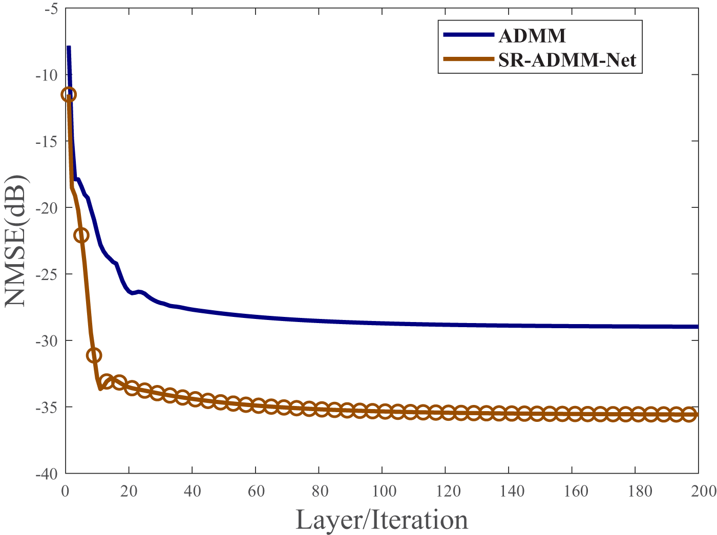
The iterative equations of the ADMM algorithm are given by (24), and the setting of the parameters in its algorithm is consistent with the initialization parameters of SR-ADMM-Net. Figure 4 shows NMSE values versus the number of network layers of the SR-ADMM-Net and the number of iterations of the ADMM algorithm under the testing set. The findings indicate that the proposed SR-ADMM-Net achieves an NMSE value of about  $-$28 dB with only about eight layers. In comparison, traditional ADMM requires more than 50 iterations to reach a final similar convergence value. Moreover, the final convergence value of SR-ADMM-Net can further drop to
 $-$35dB. These results confirm that SR-ADMM-Net achieves a faster convergence rate and higher accuracy through the automatic learning of parameters.
NMSE versus layer/iteration of SR-ADMM-Net/ADMM.

Figure 4 Long description
NMSE(dB) Layer/Iteration Legend: ADMM; SR-ADMM-Net. The horizontal axis label is Layer slash Iteration. The horizontal axis range is 0 to 200. The vertical axis label is NMSE(dB). The vertical axis range is negative 40 to negative 5. ADMM: (0, negative 8), (5, negative 18), (10, negative 23), (20, negative 26), (30, negative 27), (40, negative 27.5), (60, negative 28), (80, negative 28.3), (100, negative 28.5), (120, negative 28.6), (140, negative 28.7), (160, negative 28.8), (180, negative 28.8), (200, negative 28.8) SR-ADMM-Net: (0, negative 11), (5, negative 22), (10, negative 31), (15, negative 33), (20, negative 33.2), (30, negative 33.8), (40, negative 34.2), (60, negative 34.8), (80, negative 35.0), (100, negative 35.1), (120, negative 35.2), (140, negative 35.2), (160, negative 35.2), (180, negative 35.2), (200, negative 35.2).
2) Performance Assessment: To provide a quantitative evaluation of the target detection performance of the proposed networks, two metrics, namely the peak-to-sidelobe level ratio (PSLR) and the integrated-sidelobe level ratio (ISLR), are employed in the simulation experiments [Reference Lellouch, Mishra and Inggs46]. PSLR denotes the ratio between the highest sidelobe and the peak value, which reflects the radar’s ability to detect weak targets. PSLR in dB scale is defined as:
 \begin{equation}
\text{PSLR}=20\log (\underset{\omega \in Q,\nu \in F}{\mathop{\max }}\,(|\psi [\omega ,\nu ]|)/\psi [{{\omega }_{0}},{{\nu }_{0}}])
\end{equation}
where  $\psi$ denotes the estimated RD map,
 ${{\omega }_{0}}$ and
 ${{\nu }_{0}}$ denote the range bin and Doppler bin of target, respectively. The parameters
 $Q$ and
 $F$ define the set of range bins and Doppler bins in the RD map in addition to the main lobe. The ISLR is the ratio between the energy accumulation of the sidelobes and the peak value, which measures the energy distributed in the sidelobes. ISLR in dB scale is defined as:
 \begin{equation}
\text{ISLR}=10\log ((\sum\limits_{\omega \in Q,\nu \in F}{|\psi [\omega ,\nu ]{{|}^{2}})/(\sum\limits_{\omega \in Q,\nu \notin F}{|\psi [\omega ,\nu ]{{|}^{2}}}))}
\end{equation}
Therefore, lower PSLR and ISLR values represent better performance.
3) Simulation 2: Comparison of One-step Processing Results Between SR-ADMM-Net and SR-LSGAN: To accurately analyze the sparse coefficient estimation capability of SR-ADMM-Net and SR-LSGAN, samples with relatively high target SNRs ranging from 6 dB to  $-$4 dB, with the step of 2 dB, have been selected from the test set for the simulation experiments. Additionally, the sparse component coefficients present in the echoes are directly output for target detection through the one-step processing approach depicted in Figures 1 and 2.
Figure 5 presents the simulation results obtained from vectorized RD maps across different target SNRs, directly produced by SR-ADMM-Net and SR-LSGAN. The raw RD maps without clutter suppression are normalized via individual maximum normalization. The findings indicate that at higher target SNRs, the network’s output enables direct identification of the target and clutter. However, it is noticeable that the SR-ADMM-Net struggles to identify the target when the target SNR falls below  $-$2 dB. This limitation is attributed to the constrained discriminative ability of the sparsity prior, which does not adequately capture the sparse feature of the target. In contrast, the SR-LSGAN, which is based on generative prior, not only successfully identifies the target but also effectively estimates all clutter paths. Consequently, the capability for sparse feature extraction about both clutter and the target of SR-LSGAN is superior to that of SR-ADMM-Net.
RD maps for one-step processing of SR-LSGAN and SR-ADMM-Net for different SNR targets.

Figure 5 Long description
RD maps for one-step processing of SR-LSGAN and SR-ADMM-Net for different SNR targets. A six-by-three grid of heatmaps is shown. Column titles, left to right: Raw RD map, SR-ADMM-NET, SR-LSGAN. Row labels, top to bottom: 6dB, 4dB, 2dB, 0dB, -2dB, -4dB. All heatmaps share the same axes text. Horizontal axis label: Doppler(Hz), with tick labels -15, -10, -5, 0, 5, 10, 15. Vertical axis label: Delay Bin, with tick labels 0, 5, 10, 15, 20, 25, 30, 35. Each heatmap includes a vertical scale bar labeled Normalized Power (dB). In the Raw RD map column, the scale bar tick labels are 0, -20, -40, -60, -80, -100. In the SR-ADMM-NET and SR-LSGAN columns, the scale bar tick labels are -10, -20, -30, -40, -50, -60. The scale bars place 0 at the top for the Raw RD map column and -10 at the top for the SR-ADMM-NET and SR-LSGAN columns, with more negative values lower on the bar. Annotations inside the heatmaps use the words Clutter and Target with arrows. In the Raw RD map column for every row (6dB, 4dB, 2dB, 0dB, -2dB, -4dB), the word Clutter appears with an arrow pointing toward a narrow vertical feature aligned near Doppler 0. In the SR-ADMM-NET column, the word Target appears in the 6dB row with an arrow pointing to a small marked region near Doppler 5 and Delay Bin 10. In the 4dB row, Target is labeled near Doppler -5 and Delay Bin 10. In the 2dB row, Target is labeled near Doppler -5 and Delay Bin 10. In the 0dB row, Target is labeled near Doppler 5 and Delay Bin 10. In the -2dB row, Target is labeled near Doppler -5 and Delay Bin 10. In the -4dB row, no Target text label is visible. In the SR-LSGAN column, the word Target appears in the 6dB row with an arrow pointing to a small marked region near Doppler 5 and Delay Bin 10. In the 4dB row, Target is labeled near Doppler -5 and Delay Bin 10. In the 2dB row, Target is labeled near Doppler -5 and Delay Bin 10. In the 0dB row, Target is labeled near Doppler 5 and Delay Bin 10. In the -2dB row, Target is labeled near Doppler -5 and Delay Bin 10. In the -4dB row, Target is labeled near Doppler -5 and Delay Bin 10.
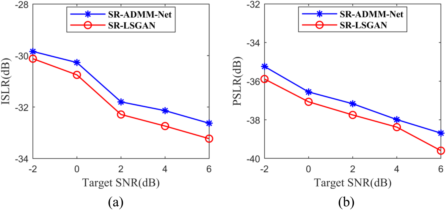
To further evaluate the target detection performance of the two methods under a one-step estimation approach, 100 Monte Carlo simulations were conducted using the test set data during the simulation experiments to calculate each metric. Figure 6 illustrates the performance curves of the metric values for the two methodologies of different target SNRs, it can be observed that the discrepancy between the metric values of the two methods is relatively minor when both methods are capable of detecting the target. At this juncture, the PSLR and ISLR values of the SR-LSGAN are approximately 0.5 dB lower than those of the SR-ADMM-Net. However, as the target SNR is progressively diminished, the SR-LSGAN maintains its capability to detect the target. Consequently, it can be concluded that the target detection performance of SR-LSGAN is markedly superior to that of SR-ADMM-Net when employing the one-step processing approach.
SR-LSGAN versus SR-ADMM-Net metric values under one-step processing with different SNR targets. (a) ISLR comparison; (b) PSLR comparison.

Figure 6 Long description
The image A showing ISLR(dB) Target SNR(dB) (a) Legend: SR-ADMM-Net, SR-LSGAN. Horizontal axis range: negative 2 to 6. Vertical axis range: negative 34 to negative 28. SR-ADMM-Net: (-2, -30), (0, -30.5), (2, -32), (4, -32.3), (6, -32.8) SR-LSGAN: (-2, -30), (0, -31), (2, -32.5), (4, -33), (6, -33.5) The image B showing PSLR(dB) Target SNR(dB) (b) Legend: SR-ADMM-Net, SR-LSGAN. Horizontal axis range: negative 2 to 6. Vertical axis range: negative 40 to negative 32. SR-ADMM-Net: (-2, -35), (0, -36.5), (2, -37.2), (4, -38), (6, -39) SR-LSGAN: (-2, -35.5), (0, -37), (2, -38), (4, -38.5), (6, -39.5).
4) Simulation 3: Comparison of Step-by-Step Estimation Results: This subsection will further analyze the detection capabilities of SR-ADMM-Net and SR-LSGAN in identifying weak targets under the step-by-step estimation approach through simulation experiments. Additionally, the performance of both methods will be compared to that of the commonly used clutter suppression algorithm, ECA-B [Reference Colone, O’Hagan, Lombardo and Baker12]. To ensure a fair and physically meaningful comparison, the RD maps with clutter suppression by ECA-B, SR-ADMM-net, and SR-LSGAN are processed with target peak normalization.
Figure 7 illustrates the simulation results of the three methods under different target SNRs, where the ECA-B algorithm is configured with 40 blocks, each containing a signal length of 4000. It is evident that the target signal is obscured within the clutter sidelobes without clutter suppression due to the direct-path signal and multipath clutter interference, making it challenging to detect. As shown in Figure 7, although SR-ADMM-Net can detect a target, some residual clutter remains, and target detection becomes increasingly challenging when the target SNR is degraded. In contrast, the SR-LSGAN and ECA-B algorithms effectively eliminated the influence of clutter, enabling clear observation of the target. However, due to the chunking process, the ECA-B algorithm may introduce blurred sub-peaks.
RD maps for step-by-step estimation for different SNR targets.

Figure 7 Long description
The image showing 24 range–Doppler heatmaps arranged as 6 signal-to-noise ratio rows by 4 method columns. Column titles: Raw RD map; ECA-B; SR-ADMM-Net; SR-LSGAN. Row labels: minus 5 decibel; minus 10 decibel; minus 15 decibel; minus 20 decibel; minus 25 decibel; minus 30 decibel. Each heatmap uses the same axes. The horizontal axis label is Doppler(Hz) with tick labels minus 15, minus 10, minus 5, 0, 5, 10, 15. The vertical axis label is Delay Bin with tick labels 0, 5, 10, 15, 20, 25, 30, 35. Each heatmap includes a vertical legend labeled Normalized Power (dB). The legend tick labels include 0, minus 20, minus 40, minus 60. The lowest tick differs by method: Raw RD map shows minus 100; ECA-B shows minus 70; SR-ADMM-Net shows minus 70; SR-LSGAN shows minus 70. The legend is a continuous gradient where higher normalized power corresponds to the upper end near 0 and lower normalized power corresponds to the lower end near the most negative value. Text annotations inside the heatmaps include the words Target and Clutter, with arrows pointing to circled regions. The circled Target regions appear at Doppler values between about minus 10 and plus 15 and Delay Bin values between about 0 and 20, depending on the row and method. The Clutter annotations point to narrow vertical features near Doppler around 0 and to other circled regions at low Delay Bin values. Across the signal-to-noise ratio rows from minus 5 decibel through minus 30 decibel, the Raw RD map column repeatedly shows a prominent narrow vertical feature near Doppler 0 with Clutter arrows and no Target label is shown in that column. In the ECA-B column, each row includes a Target label pointing to a circled region, with the circled region shifting in Doppler and Delay Bin across rows. In the SR-ADMM-Net column, each row includes both Target and Clutter labels, with Clutter arrows frequently pointing to the narrow vertical feature near Doppler 0 while Target arrows point to a separate circled region away from Doppler 0. In the SR-LSGAN column, each row includes a Target label pointing to a circled region and Clutter labels appear in some rows, including the minus 30 decibel row where both Target and Clutter labels are present.
Figure 8 shows the normalized target-range bin cuts after clutter suppression at target SNRs of  $-$25 dB and
 $-$30 dB for a more direct comparison. The findings indicate that both the SR-ADMM-Net and SR-LSGAN exhibit lower noise levels compared to the ECA-B algorithm, which are attributed to the generation of some ambiguous sub-peaks by the ECA-B algorithm. Furthermore, the noise levels associated with SR-LSGAN is marginally lower than that of SR-ADMM-Net, and SR-LSGAN demonstrates superior efficacy in filtering out clutter, effectively suppressing all or most clutter at zero frequency. Consequently, SR-LSGAN is characterized by enhanced target detection capabilities.
Normalized target range bins comparison at different SNR levels. (a) Results for  $-$25 dB target SNR; (b) results for
 $-$30 dB target SNR.

Figure 8 Long description
A two-part scientific line-plot figure labeled (a) and (b), each comparing three series in a legend: ECA-B, SR-LSGAN and SR-ADMM-Net. The image A showing a line graph. The x-axis label is Doppler (Hz), with tick labels 2, 3, 4, 5, 6, 7. The y-axis label is Normalized Power (dB), ranging from 0 at the top down to minus 50 at the bottom, with tick labels at 0, minus 5, minus 10, minus 15, minus 20, minus 25, minus 30, minus 35, minus 40, minus 45, minus 50. All three series fluctuate with repeated peaks and troughs. A prominent peak occurs near Doppler 4 Hz where the SR-ADMM-Net series reaches about 0 dB. Around the same region, the other series also rise but remain below 0 dB. Several troughs fall below minus 30 dB, including a sharp dip in the SR-LSGAN series that reaches roughly the low minus 40 dB range. Additional local peaks appear between Doppler 5 Hz and 7 Hz, with values generally between about minus 10 dB and minus 25 dB, interspersed with dips that extend below minus 30 dB. The image B showing a line graph. The x-axis label is Doppler (Hz), with tick labels minus 7, minus 6, minus 5, minus 4, minus 3, minus 2. The y-axis label is Normalized Power (dB), ranging from 0 at the top down to minus 50 at the bottom, with tick labels at 0, minus 5, minus 10, minus 15, minus 20, minus 25, minus 30, minus 35, minus 40, minus 45, minus 50. All three series fluctuate across the negative Doppler range. A prominent peak occurs near Doppler minus 3 Hz where the SR-ADMM-Net series rises to about 0 dB. Multiple deep troughs are present, including dips that approach minus 50 dB in at least one series. Between Doppler minus 7 Hz and minus 2 Hz, the curves repeatedly rise into the minus 10 dB to minus 20 dB range and fall into the minus 30 dB to minus 50 dB range, with visible separations between the three methods at several peaks and dips.
Figure 9 illustrates the metric values associated with three methodologies across different target SNRs. The results indicate that both the PSLR and ISLR values of the proposed SR-ADMM-Net and SR-LSGAN are lower than those of the ECA-B algorithm, with SR-LSGAN achieving the lowest values, both approximately 2 dB below those of the ECA-B algorithm. Additionally, the PSLR and ISLR values for SR-LSGAN and SR-ADMM-Net do not differ significantly when the target SNR falls below  $-$25 dB, which is because when the target SNR is low to a certain extent, the base of the RD map is no longer determined by the clutter sidelobe after clutter filtering, but by the noise component, resulting in no significant change in these two metrics. However, Within the target SNR range of
 $-$5 dB to
 $-$25 dB, SR-LSGAN demonstrates superior clutter filtering capabilities, with its PSLR and ISLR values being 1 dB lower than those of SR-ADMM-Net, in line with the results in the one-step processing approach. Furthermore, the observed inverse relationship between PSLR and ISLR concerning the target SNRs is consistent with the definitions of these metrics, thereby justifying the validity of the results.
Values of metrics versus different target SNRs. (a) ISLR comparison; (b) PSLR comparison.

Figure 9 Long description
The image A showing (a) ISLR (dB) versus Target SNR(dB). Horizontal axis label: Target SNR(dB). Horizontal axis range: negative 30 to negative 5. Vertical axis label: ISLR(dB). Vertical axis range: negative 35 to 0. Legend entries: ECA-B; SR-ADMM-Net; SR-LSGAN. Line markers appear as square markers for ECA-B, circle markers for SR-ADMM-Net and triangle markers for SR-LSGAN. ECA-B coordinate pairs: (negative 30, negative 5), (negative 25, negative 10), (negative 20, negative 15), (negative 15, negative 20), (negative 10, negative 25), (negative 5, negative 28). SR-ADMM-Net coordinate pairs: (negative 30, negative 6), (negative 25, negative 11), (negative 20, negative 16), (negative 15, negative 21), (negative 10, negative 26), (negative 5, negative 29). SR-LSGAN coordinate pairs: (negative 30, negative 7), (negative 25, negative 12), (negative 20, negative 17), (negative 15, negative 22), (negative 10, negative 27), (negative 5, negative 30). All three series move from (negative 30, negative 5 to negative 7) to (negative 5, negative 28 to negative 30). At each listed Target SNR(dB) value, SR-LSGAN has the lowest ISLR(dB) value, SR-ADMM-Net is between and ECA-B has the highest ISLR(dB) value. The highest ISLR(dB) values occur at Target SNR(dB) negative 30 for each series. The lowest ISLR(dB) values occur at Target SNR(dB) negative 5 for each series. The image B showing (b) PSLR (dB) versus Target SNR(dB). Horizontal axis label: Target SNR(dB). Horizontal axis range: negative 30 to negative 5. Vertical axis label: PSLR(dB). Vertical axis range: negative 40 to 0. Legend entries: ECA-B; SR-ADMM-Net; SR-LSGAN. Line markers appear as square markers for ECA-B, circle markers for SR-ADMM-Net and triangle markers for SR-LSGAN. ECA-B coordinate pairs: (negative 30, negative 10), (negative 25, negative 15), (negative 20, negative 20), (negative 15, negative 25), (negative 10, negative 30), (negative 5, negative 33). SR-ADMM-Net coordinate pairs: (negative 30, negative 11), (negative 25, negative 16), (negative 20, negative 21), (negative 15, negative 26), (negative 10, negative 31), (negative 5, negative 34). SR-LSGAN coordinate pairs: (negative 30, negative 12), (negative 25, negative 17), (negative 20, negative 22), (negative 15, negative 27), (negative 10, negative 32), (negative 5, negative 35). All three series move from (negative 30, negative 10 to negative 12) to (negative 5, negative 33 to negative 35). At each listed Target SNR(dB) value, SR-LSGAN has the lowest PSLR(dB) value, SR-ADMM-Net is between and ECA-B has the highest PSLR(dB) value. The highest PSLR(dB) values occur at Target SNR(dB) negative 30 for each series. The lowest PSLR(dB) values occur at Target SNR(dB) negative 5 for each series.
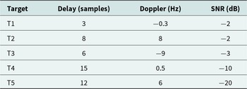
5) Simulation 4: Performance Comparison of Different Methods in Multi-Target Scenarios: A multi-target scenario experiment is performed to assess the proposed algorithms’ capabilities in sparse coefficient estimation, weak target detection, and low-Doppler target detection. It contains five targets with different SNRs and RD parameters as listed in Table 2. Specifically, T1 is a target with low-Doppler frequency and relatively high SNR  $-$2 dB, T2 is a target with the same SNR as T1 but higher Doppler frequency, T3 is a target with relatively high Doppler frequency and relatively high SNR
 $-$3 dB, T4 is a weaker target with low Doppler frequency and SNR
 $-$10 dB, and T5 is an extremely weak target with SNR
 $-$20 dB and high Doppler frequency.
Parameters of the five simulated targets

Table 2 Long description
The table lists five simulated targets with three parameters: delay in samples, Doppler shift in hertz, and signal to noise ratio in decibels. Delays range from 3 samples for T1 to 15 samples for T4, with T5 at 12 and T2 at 8. Doppler values span negative to positive, from minus 9 Hz for T3 to 8 Hz for T2; T4 is near zero at 0.5 Hz and T1 is slightly negative at minus 0.3 Hz. Signal to noise ratios are mostly low: T1 and T2 are both minus 2 dB, T3 is minus 3 dB, T4 drops to minus 10 dB, and T5 is the lowest at minus 20 dB. Compared with the others, T5 combines a relatively long delay with the poorest signal quality, while T2 has the highest positive Doppler and one of the stronger SNR values in this set. These values describe simulated conditions and do not indicate measurement uncertainty or variability beyond what is listed.
It can be seen that all five targets are masked by clutter in the raw RD map in Figure 10. Figure 11 presents the RD maps after one-step and step-by-step target detection using SR-ADMM-Net and SR-LSGAN networks. After one-step processing of the proposed networks, only T2 and strong clutter are estimated by SR-ADMM-Net in Figure 11(a), while T2, T3, and more clutter are estimated by SR-LSGAN in Figure 11(b). These results demonstrate the sparse coefficient estimation capability of both networks, with SR-LSGAN outperforming SR-ADMM-Net.
Raw RD map in multi-target scenarios.

Figure 10 Long description
Normalized Power (dB) A heatmap with a vertical axis labeled Delay Bin and a horizontal axis labeled Doppler(Hz). The horizontal axis shows tick labels at negative 15, negative 10, negative 5, 0, 5, 10 and 15. The vertical axis shows tick labels at 0, 5, 10, 15, 20, 25, 30 and 35. A vertical color scale bar is shown to the right of the heatmap. The scale is labeled Normalized Power (dB). Tick labels on the scale are 0, negative 20, negative 40, negative 60, negative 80 and negative 100. Inside the heatmap, the word Clutter appears near the left-center area. A diagonal arrow extends from the word Clutter toward a narrow vertical band near the horizontal position labeled 0 on the Doppler axis. The narrow vertical band extends upward across multiple Delay Bin values.
RD maps in multi-target scenarios. (a) SR-ADMM-Net with one-step; (b) SR-LSGAN with one-step; (c) SR-ADMM-Net with step-by-step; (d) SR-LSGAN with step-by-step.

Figure 11 Long description
The image A showing the title SR-ADMM-NET. Text at the left reads one-step. The horizontal axis label is Doppler(Hz) with tick labels from negative 15 to 15. The vertical axis label is Delay Bin with tick labels from 0 to 35. A vertical color scale at the right is titled Power (dB) with tick labels negative 20, negative 30, negative 40, negative 50, negative 60. Higher values on this scale are at negative 20 and lower values are at negative 60. Inside the plot area, arrow annotations label T3 near Doppler negative 10 and Delay Bin about 6, T1 near Doppler 0 and Delay Bin about 3, T4 near Doppler 0 and Delay Bin about 15, T5 near Doppler about 6 and Delay Bin about 13 and T2 near Doppler about 10 and Delay Bin about 9. The word Clutter appears near Doppler about negative 2 and Delay Bin about 18. Several thin oval outlines surround the labeled locations. The background is mostly uniform, with a narrow vertical feature around Doppler 0. The subfigure label (a) appears below. The image B showing the title SR-LSGAN. Text at the left reads one-step. The horizontal axis label is Doppler(Hz) with tick labels from negative 15 to 15. The vertical axis label is Delay Bin with tick labels from 0 to 35. A vertical color scale at the right is titled Power (dB) with tick labels negative 20, negative 30, negative 40, negative 50, negative 60. Higher values on this scale are at negative 20 and lower values are at negative 60. Arrow annotations label T3 near Doppler negative 10 and Delay Bin about 6, T1 near Doppler 0 and Delay Bin about 3, T4 near Doppler 0 and Delay Bin about 15, T5 near Doppler about 6 and Delay Bin about 13 and T2 near Doppler about 10 and Delay Bin about 9. The word Clutter appears near Doppler about negative 2 and Delay Bin about 18. Several thin oval outlines surround the labeled locations. The background is mostly uniform, with a narrow vertical feature around Doppler 0. The subfigure label (b) appears below. The image C showing the title SR-ADMM-NET. Text at the left reads step-by-step. The horizontal axis label is Doppler(Hz) with tick labels from negative 15 to 15. The vertical axis label is Delay Bin with tick labels from 0 to 35. A vertical color scale at the right is titled Normalized Power (dB) with tick labels 0, negative 20, negative 40, negative 60, negative 80. Higher values on this scale are at 0 and lower values are at negative 80. Arrow annotations label T3 near Doppler negative 10 and Delay Bin about 6, T1 near Doppler 0 and Delay Bin about 3, T4 near Doppler 0 and Delay Bin about 15, T5 near Doppler about 6 and Delay Bin about 13 and T2 near Doppler about 10 and Delay Bin about 9. The word Clutter appears near Doppler about negative 2 and Delay Bin about 18. Several thin oval outlines surround the labeled locations. The background shows dense variation across most Doppler and Delay Bin values and a strong vertical band is visible around Doppler 0. The subfigure label (c) appears below. The image D showing the title SR-LSGAN. Text at the left reads step-by-step. The horizontal axis label is Doppler(Hz) with tick labels from negative 15 to 15. The vertical axis label is Delay Bin with tick labels from 0 to 35. A vertical color scale at the right is titled Normalized Power (dB) with tick labels 0, negative 20, negative 40, negative 60, negative 80. Higher values on this scale are at 0 and lower values are at negative 80. Arrow annotations label T3 near Doppler negative 10 and Delay Bin about 6, T1 near Doppler 0 and Delay Bin about 3, T4 near Doppler 0 and Delay Bin about 15, T5 near Doppler about 6 and Delay Bin about 13 and T2 near Doppler about 10 and Delay Bin about 9. The word Clutter appears near Doppler about negative 2 and Delay Bin about 18. Several thin oval outlines surround the labeled locations. The background shows dense variation across most Doppler and Delay Bin values and a strong vertical band is visible around Doppler 0. The subfigure label (d) appears below. Across the four heat maps, the one-step row uses the Power (dB) scale from negative 60 to negative 20 and appears mostly uniform aside from the narrow feature near Doppler 0, while the step-by-step row uses the Normalized Power (dB) scale from negative 80 to 0 and shows widespread variation plus a prominent vertical band near Doppler 0. The labeled target markers T1 to T5 and the Clutter label appear in all four panels at the same annotated Doppler and Delay Bin locations.
To identify T1 with low-Doppler frequency, T4 with weaker SNR and low-Doppler frequency, and T5 with extremely weak SNR, step-by-step processing results of SR-ADMM-Net and SR-LSGAN are given in Figure 11(c) and (d), respectively. All five targets are clearly visible on both RD maps, demonstrating their weak target and low-Doppler target detection capabilities. Moreover, the SR-LSGAN network achieves optimal clutter suppression performance after step-by-step processing, while the sidelobes of T1 overlap with residual clutter in the SR-ADMM-Net result.
Measured results
To further demonstrate the effectiveness and superiority of the proposed method, relevant experiments are conducted using the measured data. The dataset originates from a DRM-based passive radar detection experiment, wherein the radar system receives DRM signals with an effective bandwidth of 9.7 KHz and an operating frequency of 10 MHz. The configuration of the experiment is depicted in Figure 12, with the transmitting station located off the coast of Qingdao City, Shandong Province, China, and the receiving station located off the coast of Haiyang City, Shandong Province, China, approximately 50 km apart. And the receiving station was composed of a 16-element linear array.
Experiment layout of DRM-based OFDM passive radar.

Figure 12 Long description
The map displays a section of Shandong Province, China, highlighting two key locations: Qingdao City, marked as the transmitting station (Tx) and Haiyang City, marked as the receiving station (Rx). These locations are connected by a line indicating a distance of 50 km between them. Qingdao City is situated to the southwest, near the coast, while Haiyang City is positioned to the southeast, also along the coastline. The map provides a geographical context for the placement of these stations, emphasizing their coastal proximity and the direct line of communication between them.
The processing steps for the measured data are as follows: firstly, the 16-element linear receiving array is oriented toward the transmitter direction and expected target directions to capture the reference and surveillance channel signals, respectively. Then, the measured test set samples for the networks are constructed based on processing them as presented in the signal models of Section II. Given the exceedingly low SNR of the targets within the measured data, the step-by-step estimation approach is employed for target detection, and a total of 512 OFDM symbols are used for MF to generate the RD map.
Figure 13 illustrates two distinct sets of single-field measured data experiments. As the targets in the measured data are all relatively weak, they are entirely obscured by clutter in the RD map before clutter suppression. All three methods demonstrated the capacity to effectively detect the two targets with Doppler frequencies of  $-$3.75 Hz and 4.06 Hz after clutter suppression. Additionally, Table 3 presents the PSLR and ISLR values for the two sets of measured data. The results indicate that the PSLR and ISLR values for the SR-ADMM-Net and SR-LSGAN are lower than those associated with the ECA-B algorithm, with SR-LSGAN exhibiting the lowest PSLR and ISLR values. This finding aligns with the simulation results, indicating that the proposed two SR networks exhibit superior target detection performance compared to the ECA-B algorithm.
RD maps of measured data I and II.

Figure 13 Long description
Measured data I Raw RD map A heatmap with the title “Raw RD map”. The x-axis label is “Doppler(Hz)”. The x-axis shows ticks at minus 15, minus 10, minus 5, 0, 5, 10, 15. The y-axis label is “Delay Bin”. The y-axis shows ticks at 0, 10, 20, 30, 40, 50. A vertical color scale at the right is labeled “Normalized Power (dB)”, with tick labels 0, minus 20, minus 40, minus 60, minus 80, minus 100. The plot contains a narrow vertical bright feature near Doppler 0 and low delay bins, with an arrow annotation labeled “Clutter” pointing to a bright spot near the bottom. ECA-B A heatmap with the title “ECA-B”. The x-axis label is “Doppler(Hz)”. The x-axis shows ticks at minus 15, minus 10, minus 5, 0, 5, 10, 15. The y-axis label is “Delay Bin”. The y-axis shows ticks at 0, 10, 20, 30, 40, 50. A vertical color scale at the right is labeled “Normalized Power (dB)”, with tick labels 0, minus 10, minus 20, minus 30, minus 40, minus 50, minus 60, minus 70. Two arrow annotations labeled “Target” and “Clutter” point to two bright spots near the bottom, one left of Doppler 0 and one right of Doppler 0. SR-ADMM-Net A heatmap with the title “SR-ADMM-Net”. The x-axis label is “Doppler(Hz)”. The x-axis shows ticks at minus 15, minus 10, minus 5, 0, 5, 10, 15. The y-axis label is “Delay Bin”. The y-axis shows ticks at 0, 10, 20, 30, 40, 50. A vertical color scale at the right is labeled “Normalized Power (dB)”, with tick labels 0, minus 10, minus 20, minus 30, minus 40, minus 50, minus 60, minus 70. Two arrow annotations labeled “Target” and “Clutter” point to two bright spots near the bottom, one left of Doppler 0 and one right of Doppler 0. A narrow vertical bright line is visible near Doppler 0. SR-LSGAN A heatmap with the title “SR-LSGAN”. The x-axis label is “Doppler(Hz)”. The x-axis shows ticks at minus 15, minus 10, minus 5, 0, 5, 10, 15. The y-axis label is “Delay Bin”. The y-axis shows ticks at 0, 10, 20, 30, 40, 50. A vertical color scale at the right is labeled “Normalized Power (dB)”, with tick labels 0, minus 10, minus 20, minus 30, minus 40, minus 50, minus 60, minus 70. Two arrow annotations labeled “Target” and “Clutter” point to two bright spots near the bottom, one left of Doppler 0 and one right of Doppler 0. A narrow vertical bright line is visible near Doppler 0. Measured data II Raw RD map A heatmap with no method title above it other than the column heading “Raw RD map”. The x-axis label is “Doppler(Hz)”. The x-axis shows ticks at minus 15, minus 10, minus 5, 0, 5, 10, 15. The y-axis label is “Delay Bin”. The y-axis shows ticks at 0, 10, 20, 30, 40, 50. A vertical color scale at the right is labeled “Normalized Power (dB)”, with tick labels 0, minus 20, minus 40, minus 60, minus 80, minus 100. An arrow annotation labeled “Clutter” points to a bright spot near the bottom left of Doppler 0. ECA-B A heatmap under the column heading “ECA-B”. The x-axis label is “Doppler(Hz)”. The x-axis shows ticks at minus 15, minus 10, minus 5, 0, 5, 10, 15. The y-axis label is “Delay Bin”. The y-axis shows ticks at 0, 10, 20, 30, 40, 50. A vertical color scale at the right is labeled “Normalized Power (dB)”, with tick labels 0, minus 10, minus 20, minus 30, minus 40, minus 50, minus 60, minus 70. Two arrow annotations labeled “Clutter” and “Target” point to two bright spots near the bottom, one left of Doppler 0 and one right of Doppler 0. SR-ADMM-Net A heatmap under the column heading “SR-ADMM-Net”. The x-axis label is “Doppler(Hz)”. The x-axis shows ticks at minus 15, minus 10, minus 5, 0, 5, 10, 15. The y-axis label is “Delay Bin”. The y-axis shows ticks at 0, 10, 20, 30, 40, 50. A vertical color scale at the right is labeled “Normalized Power (dB)”, with tick labels 0, minus 10, minus 20, minus 30, minus 40, minus 50, minus 60, minus 70. Two arrow annotations labeled “Clutter” and “Target” point to two bright spots near the bottom, one left of Doppler 0 and one right of Doppler 0. A narrow vertical bright line is visible near Doppler 0. SR-LSGAN A heatmap under the column heading “SR-LSGAN”. The x-axis label is “Doppler(Hz)”. The x-axis shows ticks at minus 15, minus 10, minus 5, 0, 5, 10, 15. The y-axis label is “Delay Bin”. The y-axis shows ticks at 0, 10, 20, 30, 40, 50. A vertical color scale at the right is labeled “Normalized Power (dB)”, with tick labels 0, minus 10, minus 20, minus 30, minus 40, minus 50, minus 60, minus 70. Two arrow annotations labeled “Clutter” and “Target” point to two bright spots near the bottom, one left of Doppler 0 and one right of Doppler 0. A narrow vertical bright line is visible near Doppler 0.
Metric values under the two groups of measured data

Table 3 Long description
The table reports two image quality metrics, PSLR in decibels and ISLR in decibels, for two measured datasets and three methods. For Measured Data I, ECA-B records PSLR minus 7.53 and ISLR minus 2.22, SR-ADMM-Net records minus 8.38 and minus 3.57, and SR-LSGAN records minus 8.66 and minus 4.01. For Measured Data II, ECA-B records PSLR minus 6.97 and ISLR minus 2.54, SR-ADMM-Net records minus 8.13 and minus 4.26, and SR-LSGAN records minus 8.70 and minus 4.41. In both datasets, SR-LSGAN produces the most negative values for both metrics, with SR-ADMM-Net consistently second and ECA-B highest. Comparing datasets, ECA-B improves slightly in ISLR from minus 2.22 to minus 2.54 but becomes less negative in PSLR from minus 7.53 to minus 6.97, while SR-LSGAN is nearly unchanged in PSLR and slightly more negative in ISLR. Interpretation depends on whether more negative PSLR and ISLR indicate better performance in the intended evaluation.
To further demonstrate the capability and effectiveness of the proposed networks in the application of target detection in real data, the detection results of multi-field data for the same target are also analyzed, where the consecutive multi-field RD maps and the trajectory results at the target range bin are presented. The trajectory results of the target range bin are obtained by repeating the target parameter estimation for consecutive multi-field data and displaying all the results in a single map. The consecutive multi-field RD maps over 1 minute are analyzed and the interval between two adjacent fields is 4 s. The final trajectory maps for the targets from both groups of measured data are presented in Figure 14. It is evident that SR-LSGAN and SR-ADMM-Net generate more distinct and precise trajectory maps than those of the ECA-B algorithm, particularly for measured data II, which demonstrates the versatility and superiority of the two networks in practical applications.
Trajectory maps of the targets for the two measured data sets.

Figure 14 Long description
The image shows six heatmap plots comparing target detection methods across two measured datasets. Each plot represents normalized power in decibels, indicating signal strength. The horizontal axis is labeled 'Doppler (Hz)' ranging from minus 15 to 15 and the vertical axis is labeled 'time (s)' ranging from 0 to 40. The color scale ranges from 0 to minus 50 decibels, with red indicating higher power and blue indicating lower power. The dashed rectangles represent regions of interest for target detection. Measured Data I: - ECA-B: The target track is visible within the Doppler range of approximately minus 5 to 0, showing a consistent signal over time. - SR-ADMM-Net: The target track is clearer, with reduced clutter, maintaining a strong signal in the same Doppler range. - SR-LSGAN: The target track is distinct, with better isolation and clarity, showing a strong signal throughout the time range. Measured Data II: - ECA-B: The target track appears within the Doppler range of 0 to 5, with some clutter affecting clarity. - SR-ADMM-Net: The target track is more distinct, with improved signal strength and reduced background noise. - SR-LSGAN: The target track is well-defined, showing superior isolation and clarity compared to other methods. Overall, SR-LSGAN provides the clearest and most isolated target tracks across both datasets, demonstrating superior performance in signal detection and clutter reduction.
Based on these results, subsequent estimation of parameters such as target acceleration can be further performed. However, since only the bistatic range and Doppler information of targets can be estimated from the RD spectrum, obtaining the true three-dimensional acceleration vector requires accurate calculation combined with azimuth information in subsequent processing. Notably, the network algorithm proposed in this paper preserves the phase information of the data, which can support such subsequent processing.
Conclusions
In this paper, the problem of SR for target detection in OFDM-based passive radar is investigated. Considering that the traditional iterative optimization algorithm faces challenges in selecting suitable parameters and exhibits a slow convergence rate, two SR networks, SR-ADMM-Net and SR-LSGAN, were proposed in this paper to enhance efficiency and accuracy, which utilize sparsity of data to be recovered and prior distributions learned from generative models as constraints respectively. Moreover, the one-step processing approach, which involves directly using the sparse component coefficients derived from the network output to ascertain the parameter information of the target, may result in inaccurate estimations in contexts where the target is totally masked by clutter. Consequently, a step-by-step estimation approach is proposed for detecting weak targets. Extensive experimental findings indicate that the SR-ADMM-Net demonstrates both more rapid convergence and enhanced accuracy in comparison to the ADMM algorithm. Furthermore, the proposed network exhibits lower PSLR and ISLR values relative to the ECA-B algorithm, suggesting that the target detection capabilities of both SR-ADMM-Net and SR-LSGAN surpass those of the ECA-B algorithm. Notably, the target detection performance of SR-LSGAN is marginally superior to that of SR-ADMM-Net. Finally, the measured data further confirmed the effectiveness and generality of our proposed networks.
Acknowledgements
This work was supported in part by the National Natural Science Foundation of China under Grants 62261036, and in part by the Natural Science Foundation of Jiangxi Province under Grants 20242BAB23010.
Competing interests
The authors report no conflict of interest.

Zhixin Zhao received the B.E. and Ph.D. degrees from Wuhan University, China, in 2008 and 2013, respectively. Since 2013, she has been working with the School of Information Engineering, Nanchang University, where she is currently an Associate Professor. From December 2024 to December 2025, she was a visiting scholar with Microwave Integrated Systems Laboratory (MISL), School of Electronic, Electrical and Systems Engineering, University of Birmingham, Birmingham, UK. Her main research interests include over-the-horizon radar, passive radar signal processing, and the application of deep learning in radar signal processing.

Baiming Liang was born in 2002 and is currently pursuing a bachelor’s degree in Communication Engineering at the School of Information Engineering, Nanchang University. His main research interests include radar signal processing and the application of deep learning.

Yuanshuai Chen was born in 1999 and is currently pursuing a master’s degree at the School of Information Engineering, Nanchang University. His main research interests include over-the-horizon radar, passive radar signal processing.

Huilin Zhou received the M.S. and Ph.D. degrees from Wuhan University, China, in 2002 and 2006, respectively. Since 2006, he has been working with the School of Information Engineering, Nanchang University, where he is currently a professor. His main research interests include radar systems, radar signal processing, and radar imaging.