

More than forty years of empirical research on congressional elections has documented the existence of an incumbency advantage,Footnote 1 decomposed its sources into various components of the political environmentFootnote 2 and identified its variation over time.Footnote 3 The standard conception of incumbency advantage is that the effect is purely valence.Footnote 4 According to this view, incumbency is a characteristic of a candidate, such as seniority,Footnote 5 or a resource, like the franking privilege,Footnote 6 which affects all voters’ evaluation of the candidate in an identical fashion that is independent of ideology. I argue that this standard conception obscures a key component of incumbency advantage: incumbents’ ability to develop an ideological record that is distinct from that of their parties. I show that voters have different information at their disposal about the ideological locations of candidates that varies with the candidates’ experience in office. This informational mechanism generates an incumbency advantage that systematically varies with the underlying ideological characteristics of candidates, parties and the district electorate.
The idea that incumbents can use roll-call votes in the legislature to signal ideological positions that are in line with the district and distinct from the party is not new, but its empirical relevance and effects on the incumbency advantage have yet to be systematically examined. As ArnoldFootnote 7 notes, incumbents and challengers have very different opportunities to build an ideological record: ‘House members face between 400 and 600 roll-call votes each year, and even after discounting for procedural and other minor motions, they quickly establish a long list of recorded positions. Challengers may or may not have previous records to defend, depending on what previous offices they may have held.’ Building on this insight, I develop and estimate a model to reveal the electoral importance of this difference between the informational environment of incumbents and challengers.Footnote 8
I develop an empirical model of how voters estimate the ideological location of House candidates. In the model, voters weight the candidates’ individual and party ideological positions to generate an expected candidate location, and the values of the weights are allowed to vary across levels of candidate experience.Footnote 9 I use self-reported vote intentions and candidate, party and self ideological locations to estimate the parameters of the model using the maximum likelihood estimation procedure. I then use this framework to calculate the incumbency advantage and decompose its magnitude into valence and signaling components using the estimated parameter values. Using survey data from the Cooperative Congressional Election Study (CCES) and controlling for district unobserved heterogeneity, I identify four main results.
First, I find that voter perceptions of incumbents’ ideological locations in House elections are largely based on the individual positions that incumbents take, while perceptions of challengers’ locations are heavily dependent on the party’s ideological location. Voters place an even greater party weight on the ideological positions of inexperienced challengers relative to experienced challengers. In Senate elections, there is no statistical or substantive difference between the party weights voters place on incumbents vs. challengers. Secondly, I decompose the estimated incumbency advantage into its signaling and valence components and find that the signaling mechanism explains 10–20 per cent of the incumbency advantage in House elections. I find that, consistent with the informational mechanism, the signaling effect is smaller in Senate elections, because candidates are typically better known and receive more intense media coverage than in House elections. Thirdly, I find that the incumbency advantage exhibits important cross-district heterogeneity. There is suggestive evidence of a quadratic relationship with the magnitude of incumbency advantage and district ideology: more moderate districts exhibit greater incumbency advantages. Fourthly, I investigate how interparty polarization affects the magnitude of the incumbency advantage. The empirical framework allows me to make out-of-sample predictions about the evolution of incumbency advantage for alternative variable values. I find through a series of microsimulations that the average incumbency advantage would increase by roughly 3 percentage points with a 50 per cent increase in voter perceptions of party polarization. The preferred specifications include electoral district fixed effects,Footnote 10 so the results only exploit within-district variation in candidates’ incumbency status and lend credibility to the causal interpretation of the findings.
This article contributes to three literatures. First, it is part of the vast literature on the estimation and decomposition of the incumbency advantage. Researchers have distinguished between direct officeholder benefits, quality differentials between incumbents and challengers, and the scare-off effect. I do not decompose the incumbency advantage between direct officeholder benefits, quality differentials and the scare-off effect, because this has been done in previous studies such as those conducted by Levitt and Wolfram and Hirano and Snyder.Footnote 11 Instead, I label the combination of these effects ‘valence’ because they are valued equally by all voters and do not attempt to quantify their relative importance. I supplement the previous literature by illuminating an alternative source of the incumbency advantage based on incumbents’ ability to differentiate themselves ideologically from their parties that has not received prior empirical attention.
Secondly, I contribute to the literature on how voters’ processing of ideological information operates and affects vote choice in elections.Footnote 12 In an important study, RahnFootnote 13 provides laboratory experimental evidence that fictional candidates’ partisan labels dominate issue positions in voters’ evaluations of candidates for office. In Rahn’s experimental design, the fictional candidates’ incumbency status is not manipulated across treatment and control, so there is no attempt to discern whether this information processing varies across levels of candidate experience. As discussed above, there are compelling theoretical reasons to believe that partisan labels are more informative about the ideology of relatively less-known challengers compared to incumbents. In this article, I document an important interaction between how voters interpret partisan and individual ideological information with candidates’ level of experience.Footnote 14 While partisan affiliation conveys some ideological information to voters, the magnitude of this informational effect is much more important for House challengers (both experienced and inexperienced) than for House incumbents, and I uncover no meaningful differences across challengers and incumbents in Senate contests. These empirical findings suggest a role for candidate experience in how partisan labels affect ideological inferences that has not received systematic attention in the experimental literature.
Finally, my findings contribute to the literature on the design of electoral institutions to produce electoral accountability in an environment with entrenched incumbents.Footnote 15 Many observers of American politics find the existence of an incumbency advantage normatively troubling. To the extent that incumbency advantage is due to an uneven electoral playing field between incumbents and challengers, as opposed to unmeasured differences in candidate quality,Footnote 16 its existence potentially weakens the accountability mechanism between citizens and legislators. Entrenched incumbents who are electorally insulated from competition are less responsive to citizens’ preferencesFootnote 17 and have weaker incentives to provide constituency service.Footnote 18 Holbrook and van Dunk discuss some of the large literature on the consequences of electoral competitiveness and its absence on citizens’ political participation and policy outcomes.Footnote 19
The bulk of the evidence suggests that incumbency advantage’s effects on electoral competition have a meaningful effect on the performance of American democracy. Understanding the causes of the incumbency advantage and their relative magnitudes is essential for evaluating alternative electoral rules that aim to reduce its effects in the electoral arena. Gowrisankaran, Mitchell and MoroFootnote 20 discuss a number of institutional rules, such as matching funds for challengers, mandates for equal air time, and term limits, that could reduce the welfare losses that emerge from pro-incumbent electoral bias. GersbachFootnote 21 argues that a higher vote hurdle for incumbent candidates can induce additional provision of effort on the part of elected officials and improve voter welfare in the process. Attempts to design political institutions need to account for how incumbency advantage varies across districts. The optimal re-election hurdle in a Gersbach-styleFootnote 22 model would vary with underlying district ideological characteristics.
The analysis raises several open questions about how the mechanisms documented here might apply to other political settings. While the empirical estimates are specific to the US political context, which is characterized by presidentialism and a well-defined two-party system, and the period 2006 to 2012, the mechanisms highlighted here (of voters placing weights on candidate and party positions to form ideological expectations) may occur in other political systems as well. In parliamentary systems, voters may be less concerned with the individual policy positions of legislative candidates because of their inability to cast separate votes for the executive and legislature. In political systems in which parties do not have well-defined ideologies, voters may instead place a higher weight on candidate ideology. Systematically investigating variation in individual and party weights across political contexts is a promising avenue for future research. In this article, I focus on the relatively narrow factor of candidate experience and its effect on voter information about candidate and party ideology. There are other features that may affect the relative weights that voters place on party and individual candidate ideological information, and these potential mechanisms warrant attention in future research. In particular, contested primaries, marked by higher levels of media coverage and campaign advertising, may provide more information about candidates that persists until the general election. Similarly, high levels of congruence between media markets and congressional districtsFootnote 23 may produce citizens who have more information about congressional candidates’ ideologies.
The remainder of the article is organized as follows. In the next section, I describe the empirical framework that guides the estimation. In the third section, I describe the CCES and candidate experience data that I employ to estimate the model. In the fourth section, I present the main results. I examine the model fit relative to other alternative models. In the fifth section, I examine how the estimated incumbency advantage varies across districts and provide evidence that incumbency advantage is higher in ideologically moderate districts. I then investigate how out-of-sample changes in interparty polarization would affect the magnitude of the incumbency advantage. I also motivate and discuss a series of robustness checks, which are included in the online appendix. The final section concludes.
EMPIRICAL FRAMEWORK
Two candidates, one with a Democratic and one with a Republican affiliation, are competing for election in each district, d=1,…, D at time periods t=1,…, T. Each candidate campaigns by announcing an ideological locationFootnote 24 in a unidimensional policy space. Voters are uncertain about the exact ideological location of candidates in the policy space.
Each candidate’s ideal policy is unknown to the voter. The voter, indexed by n, estimates a Democratic candidate’s ideological location,
 $$\hat{x}_{{ndt}}^{{Dem}} $$
, as a linear function of the voter’s perception of the party’s position,
 $$x_{{ndt}}^{{Dem}} $$
, and the candidate’s position,
 $$\tilde{x}_{{ndt}}^{{Dem}} $$
. The voter places a weight of λ on the party’s location and 1−λ on the candidate’s position. I allow the relative weight placed on the party location to vary across levels of candidate experience. In the empirical analysis, I allow each of these parameters to take on three distinct values, λ
I
, λ
EC
, λ
IEC
where the subscripts refer to incumbents, experienced challengers and inexperienced challengers.Footnote
25
Hence, in House elections λ is a 3×1 vector of coefficients where each element corresponds to a distinct level of candidate experience and
 $x_{{ndt}}^{{Dem}} $
and
 $$\tilde{x}_{{ndt}}^{{Dem}} $$
are each 3×1 vectors of candidate and party positions that take on a value of 0 when a candidate does not possess the relevant experience level at t.
 $$\hat{x}_{{ndt}}^{{Dem}} \,{\equals}\,\lambda \prime x_{{ndt}}^{{Dem}} {\plus}\left( {1{\minus}\,\lambda \prime} \right)\tilde{x}_{{ndt}}^{{Dem}} $$
The function for Republican candidates is defined analogously. To estimate the weights that voters place on candidates’ ideological locations, I more completely specify the voter’s utility function. Voters have symmetric preferences with a unique ideal point in the policy space,
 $x_{{ndt}}^{{\asterisk}} $
. Voters’ utility is determined by both the ideological distance between their ideal points and the location of the candidate and non-policy characteristics of the candidate and the election year. Consistent with the empirical findings of Berinsky and Lewis,Footnote
26
I specify a linear absolute loss function for the policy component of the voter’s utility function:
 $$U\left( {\hat{x}_{{ndt}}^{{Dem}} ,x_{{ndt}}^{{\asterisk}} } \right)\,{\equals}\,{\minus}\gamma \left| {\hat{x}_{{ndt}}^{{Dem}} } \right.{\minus}\,\left. {x_{{ndt}}^{{\asterisk}} } \right|{\plus}\delta \prime Exp_{{dt}}^{{Dem}} {\plus}\alpha _{d} {\plus}v_{t} {\plus}\beta \prime z_{{ndt}} {\plus}\zeta _{{ndt}} $$
The
 $Exp_{{dt}}^{{Dem}} $
are candidate valence levels that are operationalized using the vector of candidate experience dataFootnote
27
and δ is a vector of coefficients on candidate experience. The γ parameter allows the importance of policy relative to non-policy factors to vary, with the limiting case being γ=0 and policy having no effect on voter decisions. The α
d
are district fixed effects that accommodate unobservable cross-district variation in the propensity to support the Democratic candidate, the v
t
are year fixed effects that account for national partisan swings,Footnote
28
z
ndt
is a column vector of K observable individual-level demographic characteristics that affect the probability of voting for the Democratic candidate, and β is a K by 1 vector of coefficients.Footnote
29
The ζ
ndt
is a voter-specific idiosyncratic and unobservable preference shock that is orthogonal to the covariates. In the base specification, I do not allow respondent self-identified partisanship to affect the voter’s utility for the two candidates, but instead posit ideology as the primitive that affects the probability of vote choice. In a robustness check, I allow the respondent’s utility for each candidate to vary with the respondent’s self-identified partisanship.
The voter selects the Democratic candidate if the utility from the Democrat exceeds the utility from the Republican:
 $$\eqalignno{ U\left( {\hat{x}_{{ndt}}^{{Dem}} ,x_{{ndt}}^{{\asterisk}} } \right) & \,{\equals}\,{\minus}\gamma \left| {\hat{x}_{{ndt}}^{{Dem}} } \right.{\minus}\,\left. {x_{{ndt}}^{{\asterisk}} } \right|{\plus}\delta \prime Exp_{{dt}}^{{Dem}} {\plus}\alpha _{d} {\plus}v_{t} {\plus}\beta \prime z_{{ndt}} {\plus}\zeta _{{ndt}} \cr & \quad\,\gt\,{\minus}\gamma \left| {\hat{x}_{{ndt}}^{{Rep}} } \right.{\minus}\,\left. {x_{{ndt}}^{{\asterisk}} } \right|{\plus}\delta \prime Exp_{{dt}}^{{{\mathop{ Re}\nolimits} p}} {\equals}\,U\left( {\hat{x}_{{ndt}}^{{Dem}} ,x_{{ndt}}^{{\asterisk}} } \right) $$
In the base specification, I assume that the ζ ndt are identically and independently distributed normally with mean 0 and variance 1 to generate a probit model for the voter’s choice probability. After rearranging the inequality in Equation 1 and using the symmetry of the normal probability density, the probability that the voter chooses the Democratic candidate is then given by:
 $$\eqalignno{ & {\ Pr}_{{ndt}} \left( {{\rm Vote\,\,Dem}} \right) \,{\equals}\, \Phi \left( {{\minus}\gamma \left| {\hat{x}_{{ndt}}^{{Dem}} } \right.{\minus}\,\left. {x_{{ndt}}^{{\asterisk}} } \right|{\plus}\gamma \left| {\hat{x}_{{ndt}}^{{{\mathop{ Re}\nolimits} p}} } \right.{\minus}\,\left. {x_{{ndt}}^{{\asterisk}} } \right|{\plus}\delta \prime\left( {Exp_{{dt}}^{{Dem}} {\minus}\,Exp_{{dt}}^{{{\mathop{ Re}\nolimits} p}} } \right){\plus}\alpha _{d} {\plus}v_{t} {\plus}\beta \prime z_{{ndt}} } \right) $$
The likelihood function over voters, electoral districts and election cycles is then:
 $$\eqalignno{ & {\cal L} {{}} \left( {{\rm Vote\,Dem}_{{ndt}} ;\,\alpha ,\beta ,\delta ,\gamma ,\lambda ,v} \right)\, \cr & {\equals} \mathop{\prod}\limits_{t} \mathop{\prod}\limits_{d} \mathop{\prod}\limits_{n} Pr_{{ndt}} \left( {{\rm Vote\,\,Dem}} \right)^{{{\rm Vote\,\,Dem}_{{ndt}} }} \left {(1{\minus}\,Pr_{{ndt}} \left( {{\rm Vote\,\,Dem}} \right))^{{1{\minus}{\rm Vote\,\,Dem}_{{ndt}} }} } \right $$
I estimate the parameters by maximizing the likelihood function, and compute the standard errors with the block bootstrapFootnote 30 where the blocks are defined as districts in House elections and states in Senate elections. To implement the block bootstrap, I draw a sample of districts or states with replacement, where the number of drawn districts or states in the bootstrap replication sample is equal to the total number of districts of states in the true sample. I then estimate the parameters of the model on the resulting bootstrap sample. I repeat this procedure 250 times for 250 block bootstrap replications and then calculate the standard deviation of the coefficient estimates across the 250 replications. The resulting standard deviation is my estimate of the standard errors.Footnote 31 The purpose of the block bootstrap is to allow for arbitrary correlation in the error terms within districts or states; it is analogous to clustering the standard errors at the district or state level in a closed-form calculation of the standard errors. I separately estimate the parameters for House and Senate elections.
The framework advanced here is motivated by the belief that voter information about candidate ideology systematically varies with the level of candidate experience, and that there may be important differences in these patterns across House and Senate elections. In the online appendix, I directly investigate this possibility using a series of district fixed effects regressions on how survey respondents’ information about candidate ideology varies with candidate experience. In House contests, respondents are more willing to estimate candidate ideology when the candidate is an incumbent than when he or she is either an experienced or inexperienced challenger. In Senate contests, the pattern is more ambiguous. I also find that the variability of the candidate ideology estimates within a candidate-district-year is smaller for incumbents and experienced challengers relative to inexperienced challengers in House contests. These results illustrate that in House contests there is systematic and monotonic variation in voter information about candidate ideology with respect to the level of candidate experience and less of a systematic pattern in Senate elections.
The framework allows me to decompose the incumbency advantage into valence and signaling components. The total incumbency advantage represents the difference in average vote share between an incumbent standing for re-election and the counterfactual, in which the incumbent is replaced by a challenger (either experienced or inexperienced). I now define the incumbency advantage and its valence and signaling components for the case of a Democratic incumbent being replaced by an inexperienced challenger. Other incumbency advantages, such as a Republican incumbent being replaced by a Republican experienced challenger, are defined analogously. Let
 $$Pr\left( {{\rm Vote\,\,Dem}_{{ndt}}^{C} \left( {{\Bbb 1}_{{ndt}}^{{DemIEC}} {\equals}1} \right)\left| {{\Bbb 1}_{{ndt}}^{{DemI}} } \right.{\equals}1} \right)$$
denote the counterfactual vote probability of a Democratic incumbent who is replaced by a Democratic inexperienced challenger. Similarly, let
 $$Pr\left( {{\rm Vote\,\,Dem}_{{ndt}}^{{CV}} \left( {{\Bbb 1}_{{ndt}}^{{DemIEC}} {\equals}1} \right)\left| {{\Bbb 1}_{{ndt}}^{{DemI}} } \right.{\equals}1} \right)$$
denote the counterfactual vote probability of a Democratic incumbent who is replaced by a Democratic inexperienced challenger, but holding the signaling parameters constant at their incumbent values and changing the valence parameters to those of an inexperienced challenger.
 $$Pr\left( {{\rm Vote\,\,Dem}_{{ndt}}^{{CS}} \left( {{\Bbb 1}_{{ndt}}^{{DemIEC}} {\equals}1} \right)\left| {{\Bbb 1}_{{ndt}}^{{DemI}} } \right.{\equals}1} \right)$$
is the signaling counterfactual in which the valence parameters are held constant and the signaling parameters are changed to their inexperienced challenger level. The total district respondent-weighted incumbency advantage for district d is:Footnote
32
 $$\eqalignno{ {\rm Total}\,{\rm Inc}\,{\rm Adv}_{d} & \,{\equals}\, {1 \over {N_{d} }}\mathop{\sum}\limits_{n\,{\equals}\,1}^{N_{d} } {Pr } ({\rm Vote\,\,Dem}_{{ndt}} \left| {{\Bbb 1}_{{ndt}}^{{DemI}} {\equals}1} \right.){\minus} Pr ({\rm Vote\,\,Dem}_{{ndt}}^{C} ({\Bbb 1}_{{ndt}}^{{DemIEC}} {\equals}1)\left| {{\Bbb 1}_{{ndt}}^{{DemI}} {\equals}1} \right.) \cr & {\equals} {1 \over {N_{d} }}\mathop{\sum}\limits_{n\,{\equals}\,1}^{N_{d} } \Phi ({\minus}\left| {\lambda \prime x_{{ndt}}^{{Dem}} } \right.{\plus}(1{\minus}\,\lambda \prime)\tilde{x}_{{ndt}}^{{Dem}} {\minus}\,\left. {x_{{ndt}}^{{\asterisk}} } \right|{\plus}\left| {\lambda \prime x_{{ndt}}^{{{\mathop{ Re}\nolimits} p}} } \right.{\plus}(1{\minus}\,\lambda \prime)\tilde{x}_{{ndt}}^{{{\mathop{ Re}\nolimits} p}} {\minus}\,\left. {x_{{ndt}}^{{\asterisk}} } \right| \cr & {\plus}\hat{\delta }\prime(Exp_{{dt}}^{{Dem}} {\minus}Exp_{{dt}}^{{{\mathop{ Re}\nolimits} p}} ) {\plus}\hat{\alpha }_{d} {\plus}\hat{v}_{t} {\plus}\left. {\hat{\beta }\prime z_{{ndt}} } \right|{\Bbb 1}_{{ndt}}^{{DemI}} \,{\equals}\,1) {\minus}\Phi ({\minus}\left| {\lambda \prime x_{{ndt}}^{{DemIEC}} } \right.{\plus}(1{\minus}\,\lambda \prime)\tilde{x}_{{ndt}}^{{DemIEC}} \cr & {\minus}\left. {x_{{ndt}}^{{\asterisk}} } \right|{\plus}\left| {\lambda \prime x_{{ndt}}^{{{\mathop{ Re}\nolimits} p}} } \right.{\plus}(1{\minus}\lambda \prime)\tilde{x}_{{ndt}}^{{{\mathop{ Re}\nolimits} p}} \,{\minus}\,\left. {x_{{ndt}}^{{\asterisk}} } \right|{\plus}\hat{\delta }\prime(Exp_{{dt}}^{{DemIEC}} {\minus}\,Exp_{{dt}}^{{{\mathop{ Re}\nolimits} p}} ) \cr & {\plus}\hat{\alpha }_{d} {\plus}\hat{v}_{t} {\plus}\left. {\hat{\beta }\prime z_{{ndt}} } \right|{\Bbb 1}_{{ndt}}^{{DemI}} {\equals}1) $$
This approach allows me to decompose the portion of the incumbency advantage that is due to valence and signaling. The valence component is defined by holding the party weight variables constant and varying the valence variables:
 $$\eqalignno{ {\rm Valence}\,{\rm Inc}\,{\rm Adv}_{d} \,{\equals}\, & {1 \over {N_{d} }}\mathop{\sum}\limits_{n\,{\equals}\,1}^{N_{d} } {Pr} ({\rm Vote\,\,Dem}_{{ndt}} \left| {{\Bbb 1}_{{ndt}}^{{DemI}} {\equals}1} \right.){\minus}Pr({\rm Vote\,\,Dem}_{{ndt}}^{{CV}} ({\Bbb 1}_{{ndt}}^{{DemIEC}} )\left| {{\Bbb 1}_{{ndt}}^{{DemI}} {\equals}1} \right.) \cr & {\equals}\,{1 \over {N_{d} }}\mathop{\sum}\limits_{n\,{\equals}\,1}^{N_{d} } \Phi ({\minus}\left| {\lambda \prime x_{{ndt}}^{{Dem}} } \right.{\plus}(1{\minus}\,\lambda \prime)\tilde{x}_{{ndt}}^{{Dem}} {\minus}\,\left. {x_{{ndt}}^{{\asterisk}} } \right|{\plus}\left| {\lambda \prime x_{{ndt}}^{{Rep}} } \right.{\plus}(1{\minus}\,\lambda \prime)\tilde{x}_{{ndt}}^{{Rep}} {\minus}\,\left. {x_{{ndt}}^{{\asterisk}} } \right| \cr & {\plus}\hat{\delta }\prime(Exp_{{dt}}^{{Dem}} {\minus}Exp_{{dt}}^{{Rep}} ){\plus}\hat{\alpha }_{d} {\plus}\hat{v}_{t} {\plus}\left. {\hat{\beta }\prime z_{{ndt}} } \right|{\Bbb 1}_{{ndt}}^{{DemI}} {\equals}1) \cr & {\minus}\Phi ({\minus}\left| {\lambda\ {\!}{\!} ^{I}x_{{ndt}}^{{Dem}} } \right. {\plus}(1 {\minus}\lambda ^{I})\tilde{x}_{{ndt}}^{{Dem}} {\minus}\left. {x_{{ndt}}^{{\asterisk}} } \right|{\plus}\left| {\lambda x_{{ndt}}^{{Rep}} } \right.{\plus}(1{\minus}\,\lambda )\tilde{x}_{{ndt}}^{{Rep}} {\minus}\,\left. {x_{{ndt}}^{{\asterisk}} } \right| \cr & {\plus}\hat{\delta }\prime(Exp_{{dt}}^{{DemIEC}} {\minus}Exp_{{dt}}^{{Rep}} ) {\plus}\hat{\alpha }_{d} {\plus}\hat{v}_{t} {\plus}\left. {\hat{\beta }\prime z_{{ndt}} } \right|{\Bbb 1}_{{ndt}}^{{DemI}} {\equals}1) $$
Similarly, the signaling component of the incumbency advantage is defined by varying the party weight parameters to reflect the counterfactual in which the Democratic incumbent is replaced by an inexperienced challenger and holding the valence parameters constant:
 $$\eqalignno{ {\rm Signaling}\,{\rm Inc}\,{\rm Adv}_{d} & \,{\equals}\, {1 \over {N_{d} }}\mathop{\sum}\limits_{n\,{\equals}\,1}^{N_{d} } {Pr\left( {{\rm Vote\,\,Dem}_{{ndt}} \left| {{\Bbb 1}_{{ndt}}^{{DemI}} {\equals}1} \right.} \right){\minus}Pr\left( {{\rm Vote\,\,Dem}_{{ndt}}^{{CS}} \left( {{\Bbb 1}_{{ndt}}^{{DemIEC}} {\equals}\,1} \right)\left| {{\Bbb 1}_{{ndt}}^{{DemI}} {\equals}\,1} \right.} \right)} \cr & {\equals}\,{1 \over {N_{d} }}\mathop{\sum}\limits_{n\,{\equals}\,1}^{N_{d} } \Phi ({\minus}\left| {\lambda \prime x_{{ndt}}^{{Dem}} } \right.{\plus}\left( {1{\minus}\,\lambda \prime} \right)\tilde{x}_{{ndt}}^{{Dem}} {\minus}\,\left. {x_{{ndt}}^{{\asterisk}} } \right|\lambda \prime x_{{ndt}}^{{Rep}} {\plus}\left( {1{\minus}\,\lambda \prime} \right)\tilde{x}_{{ndt}}^{{Rep}} \cr & {\minus}\left. {x_{{ndt}}^{{\asterisk}} } \right|\hat{\delta }\prime\left( {Exp_{{dt}}^{{Dem}} {\minus}\,Exp_{{dt}}^{{Rep}} } \right){\plus}\hat{\alpha }_{d} {\plus}\hat{v}_{t} {\plus}\left. {\hat{\beta }'z_{{ndt}} } \right|{\Bbb 1}_{{ndt}}^{{DemI}} {\equals}\,1) \cr & {\minus}\,\Phi \left( {{\minus}\left| {\lambda \prime x_{{ndt}}^{{DemIEC}} } \right. {\plus}\left( {1{\minus}\,\lambda \prime} \right)\tilde{x}_{{ndt}}^{{DIEC}} {\minus}\left. {x_{{ndt}}^{{\asterisk}} } \right| {\plus}\left| {\lambda \prime x_{{ndt}}^{{Rep}} } \right.{\plus}\left( {1{\minus}\,\lambda \prime} \right)\tilde{x}_{{ndt}}^{{Rep}} {\minus}\,\left. {x_{{ndt}}^{{\asterisk}} } \right| } \right \cr & {\plus}\hat{\delta }\prime\left( {Exp_{{dt}}^{{Dem}} {\minus}Exp_{{dt}}^{{Rep}} } \right)\hat{\alpha }_{d} {\plus}\hat{v}_{t} {\plus}\left. {\hat{\beta }\prime z_{{ndt}} } \right|{\Bbb 1}_{{ndt}}^{{DemI}} {\equals}1 \big)} $$
Note that the valence and signaling components do not necessarily sum to equal the total incumbency advantage due to the nonlinearity of the normal cumulative distribution function.Footnote 33 To construct a legislature-wide estimate of the incumbency advantage and its components, I weight each district or state equally.Footnote 34 As the framework makes clear, there are a variety of theoretically distinct incumbency advantages that the empirical literature has generally not distinguished from one another. My primary interest is in the incumbency advantage defined by the counterfactual in which an incumbent candidate is replaced by a challenger so that both candidates lack the advantages of incumbency. This is the appropriate counterfactual for analyzing an institutional reform such as a one-term limit. An alternative incumbency advantage is defined by the counterfactual in which challengers are given the advantages of incumbency. This is the appropriate counterfactual for analyzing an institutional reform such as matching the level of campaign expenditures of challengers with those of incumbents.
DATA
The CCES serves as my primary source of data on vote choice, voter information and individual demographics. It surveys approximately 30,000 individuals each electoral cycle asking them a wide variety of political questions, including their vote intentions in the 2006, 2008, 2010 and 2012 congressional elections.Footnote 35 In the 2012 House elections, some respondents are drawn into new districts with potentially different incumbent candidates than in 2010 due to decennial redistricting. Even though a candidate is an incumbent, they may not be as well known to these ‘new voters’Footnote 36 and the party informational weights might be higher as a result for this subset of voters. As a robustness check, I restrict the estimation to the sample of House districts from 2006–10 and find very similar results.
I merge these survey data with Gary Jacobson’s data on candidate experience in House elections.Footnote 37 Since this data include information on whether a challenger has previously held state elective office, I employ this measure of candidate experience in my empirical analysis. I allow the information parameters to vary across inexperienced and experienced challengers in all of the models. I separately estimate models for House and Senate elections. While Jacobson’s data on candidate experience covers all House elections in the sample, I do not have data on whether Senate candidates have previously held state-level elective office. For Senate elections, I therefore classify all non-incumbent candidates as challengers.Footnote 38 Instead of pooling House and Senate elections, I estimate the model separately on each set of data and allow the parameters to vary arbitrarily across elections for both chambers.
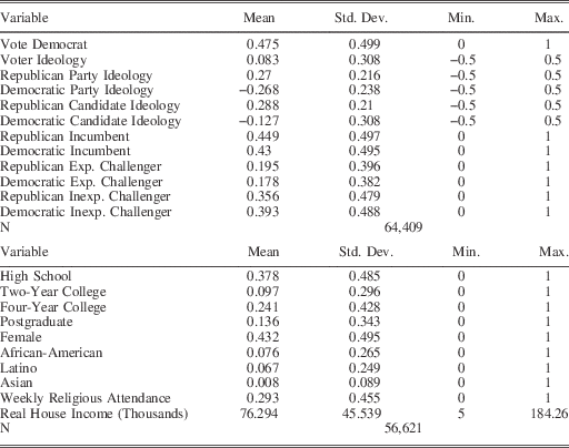
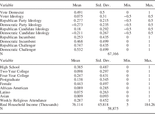
I restrict the main estimation sample in two ways. First, I remove all elections that are unopposed or only have one major party candidate.Footnote 39 Secondly, I remove all respondents who do not report an estimate for the ideological location of the major party candidates and parties. For specifications that include respondent demographics as covariates, I drop observations in which one or more of the covariates is missing. Tables 1 and 2 report summary statistics for the sample for House and Senate elections.
House Summary Statistics

Senate Summary Statistics

The article heavily leverages the self-reported ideological locations of voters and their estimates of candidate locations. While I cannot directly validate voters’ ability to place themselves and candidates in an ideological space, I can examine whether these self and candidate placements are correlated with other commonly used measures of ideology to assess the external validity of these measures. In the online appendix, I report scatter plots of the mean CCES self-reported ideology and Tausanovitch and Warshaw’sFootnote 40 multilevel regression with post-stratification (MRP) measure of district ideology derived from public opinion surveys. To investigate whether CCES respondents are able to locate candidates in the ideological space, I use Bonica’sFootnote 41 Campaign Finance (CF) scores as the measure of candidate ideology and examine its relationship with the average CCES ideological placement for each candidate.Footnote 42 The correlation between mean district CCES self-reported ideology and the MRP measure is 0.8444 in the House and 0.7644 in the Senate, and the correlation between mean district placements of candidates and Bonica’s CF scores is 0.8446 in the House and 0.8249 in the Senate. These aggregate results suggest that CCES respondents’ placements are meaningful measures of ideology that are systematically related to other measures of ideology used in the literature.Footnote 43 However, it is important to note that I do not use these aggregate measures in the estimation; I only use individual-level ideological estimates in the discrete choice model. If there are systematic differences across respondents in how they define the ideological scale, using aggregate data might be misleading.
The CCES solicits a large number of respondent-specific demographic and political characteristic from respondents. I include a large number of these responses as additional control covariates in the analysis. I include indicators for female, African-American, Latino, Asian, attends religious services weekly and the highest level of educational attainment (high school degree, two-year college degree, four-year college degree, post-graduate degree). I also include respondent-reported household income. The CCES asks respondents to report their income as a categorical variable defined by income ranges, which are not standard across the survey waves. I therefore take the midpoint of the nominal income categories. For top-coded values above $150,000, I fix nominal income at $175,000. I then adjust the nominal income levels using the Consumer Price Index and express all dollar amounts in real 2012 terms. In the online appendix, I report the CCES question numbers for all variables used in the estimation.
RESULTS
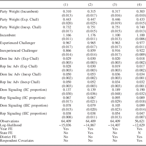
Table 3 reports the coefficient estimates and incumbency advantage quantities for House elections. The top portion of the table reports the estimated coefficients from the maximum likelihood vote choice model. The first column reports results from the base specification with only year fixed effects. The second column adds state fixed effects to the specification. The third column includes House district fixed effects, which are the most credibly identified regression results. The specification with district fixed effects relies on within-district variation in candidates’ incumbency status to identify the parameter estimates. As an additional robustness check, in the fourth column I include the complete set of individual demographic covariates described above.Footnote 44
House Elections

Note: parameter estimates and incumbency advantage estimates for House elections. Block bootstrap standard errors in parentheses are clustered at the district level.
Two striking patterns are revealed in the table. First, the party weights that voters use to estimate the ideological location of inexperienced challengers are dramatically higher than those for incumbents and experienced challengers. Across the four specifications, the party weights range from 0.732 to 0.751 for inexperienced challengers, 0.433 to 0.447 for experienced challengers, and 0.303 to 0.317 for incumbents. These results are very stable across the alternative model specifications and are precisely estimated. I reject the null that any of the informational weights are equal.Footnote 45 Secondly, incumbents have the highest conditional probability of winning a citizen’s vote, followed by experienced challengers and then inexperienced challengers. This monotonic ordering of conditional vote probability with candidate experience is consistent with a wide array of previous research.Footnote 46 Again, the point estimates are quite stable across the specifications. The presence of district fixed effects and respondent-level covariates does not exert a large influence on these coefficient point estimates, but the model fit improves appreciably with these variables, as evidenced by the decrease in the log-likelihood.
The bottom portion of Table 3 displays the House average estimated incumbency advantage and its decomposition broken out separately for Republican and Democratic candidates relative to both experienced and inexperienced challengers. An incumbent’s electoral advantage relative to an inexperienced challenger ranges from approximately 3.2 to 5.3 percentage points and relative to an experienced challenger from approximately 1.7 to 3 percentage points across the specifications. These magnitudes are somewhat smaller than the roughly 5–10 percentage points typically estimated in the literature using post-World War II House elections.Footnote 47 However, in recent work JacobsonFootnote 48 finds that the incumbency advantage has declined significantly since 2000, reaching a low of 3–3.7 percentage points in the 2014 cycle. Despite using individual survey data, as opposed to aggregate election returns, and employing a very different estimation approach, my estimates of the incumbency advantage from 2006–2012 are quite consistent with Jacobson’s findings. While the party weight and experience effects are extremely stable even when district fixed effects are added to the specification, the incumbency advantage results are more variable across the specifications. In the analysis below that uses estimated incumbency advantage, I rely on the preferred specification that includes district fixed effects and respondent-level covariates.
The final four rows of the tables display the proportion of the incumbency advantage that is attributable to the ideological signaling mechanism. In the preferred specification, which includes district fixed effects and individual covariates, the proportion of the incumbency advantage relative to experienced challengers explained by the signaling mechanism is 0.19 for Democratic candidates and 0.089 for Republican candidates. The proportion of the incumbency advantage relative to inexperienced challengers that is explained by the signaling mechanism is smaller: 0.099 for Democratic candidates and 0.047 for Republican candidates. While the Democratic and Republican estimated incumbency advantages are very close to one another within each specification, the cross-party differences are starker for the signaling decomposition. Democratic incumbents derive approximately twice as much of their incumbency advantage from the signaling mechanism as Republican candidates. One potential explanation for this finding is the difference in how the average voter evaluates the ideology of his or her Democratic House candidate compared to that of the Democratic party as a whole. As revealed in Table 1, the average CCES respondent in the sample places the Democratic Party at −0.268 while the Democratic candidate is located at the more moderate −0.127. In contrast, the average voter locates Republican candidates at 0.288 and the Republican Party at 0.27. As reflected in the incumbency advantage decomposition, incumbents’ greater ability to separate themselves from the party is more valuable for Democratic House candidates.
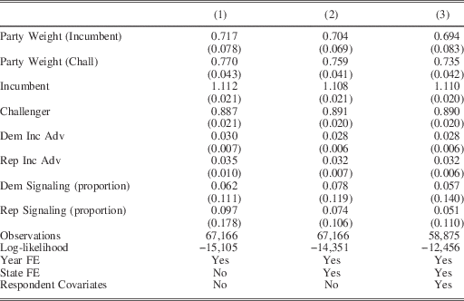
Table 4 reports the coefficient estimates and incumbency advantage quantities for the Senate. The table is organized identically to the House table, except, as discussed above, I do not have data on whether a Senate challenger is experienced or inexperienced and therefore only include state fixed effects in the estimation. The first column reports the base specification with only year fixed effects. The second column reports the specification with state fixed effects and the third column results include individual respondent demographics in the estimation.
Senate Elections

Note: parameter estimates and incumbency advantage estimates for Senate elections. Block bootstrap standard errors in parentheses are clustered at the state level.
There are several important differences between the House and Senate results. First, the party weights for Senate incumbents are substantially larger than the party weights in the House. Secondly, the difference in party weights between incumbents and challengers is trivially small and statistically insignificant. Both of these results are consistent with a more nationalized electoral environment in Senate electoral contests. Most importantly, the proportion of the incumbency advantage that is attributable to the signaling mechanism is only about 0.05, which is substantially lower than in House contests. Additionally, the proportions of incumbency advantage that are attributable to the signaling mechanism for Republican and Democratic candidates are much closer to one another than in the case of the House elections. Recall that in House elections, voters believe that the Democratic Party is significantly to the left of the average Democratic candidate, but do not have similar beliefs about Republican candidates. In Senate contests there is no such asymmetry between Democratic and Republican candidates.
MODEL FIT
Before quantifying cross-district variation in incumbency advantage, I evaluate the model fit of the ideological signaling model relative to two plausible alternative specifications. First, I consider the possibility that voters do not use information about candidates’ ideologies in their voting decisions. This corresponds to setting γ=0 in Equation 1. Under this scenario, voters only evaluate candidates based on their valence and the additional covariates that predispose the voter toward either the Democratic or Republican candidate. I fix γ=0 and estimate the remaining parameters by maximizing the constrained likelihood function. I refer to this specification as the no policy model. The no policy model is an important benchmark to investigate. Some scholars argue that ideological positions play a small role in congressional elections compared to other factors.Footnote
49
Secondly, I consider the possibility that the voter’s reported value of the candidate’s location on the CCES is actually the weighted estimate,
 $$\hat{x}_{{ndt}} $$
, as opposed to the voter’s perception of the candidate’s position,
 $$\tilde{x}_{{ndt}} $$
. To operationalize this model I use the voters’ reported location of the Democratic and Republican candidates for
 $\hat{x}_{{ndt}}^{{Dem}} $
and
 $\hat{x}_{{ndt}}^{{Rep}} $
in Equation 1. I refer to this specification as the alternative information model.Footnote
50
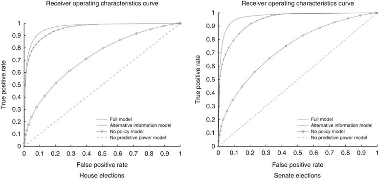
I use the fitted probabilities of the full model and the no policy and alternative information models to classify each CCES respondent as a predicted vote for the Democratic or Republican candidate, and then plot the receiver operating characteristics curve for each model.Footnote 51 Receiver operating curves that are more bowed out relative to the 45 degree line have higher explanatory power than models with less area under the curve.
As shown in the receiver operating characteristic graphs in Figure 1, the ideological signaling model has the best classification success of the three models in both House and Senate elections. While even the no policy model performs notably better than a model with no predictive power, adding the policy preferences of voters and candidates to the utility function significantly improves the accuracy of the classification. The alternative information model, in which voters use their self-reported candidate locations as the posterior estimates, performs better than the no policy model, but is notably worse than the ideological signaling model. Comparing the House and Senate, we see only minor differences between the two chambers; the alternative information model performs slightly better in House elections.
Receiver operating characteristics curve for classification accuracy of survey respondents’ reported vote intention in House and Senate elections Note: the graphs are based on the fitted probabilities of three competing models: the full ideological signaling model, the no policy model (in which the γ parameter in the voter’s utility function is set equal to 0) and the alternative information model (in which the voter’s posterior estimate of the candidate’s location is set at the reported value instead of the weighted value). All three curves are based on models estimated with the full set of district fixed effects and respondent demographic characteristics. The curves plot the false positive rate against the true positive rate for alternative classification cut-off values. The dashed line at 45 degrees is the no discrimination line that would prevail for a model that had no classification accuracy.

THE CROSS-SECTION OF INCUMBENCY ADVANTAGE
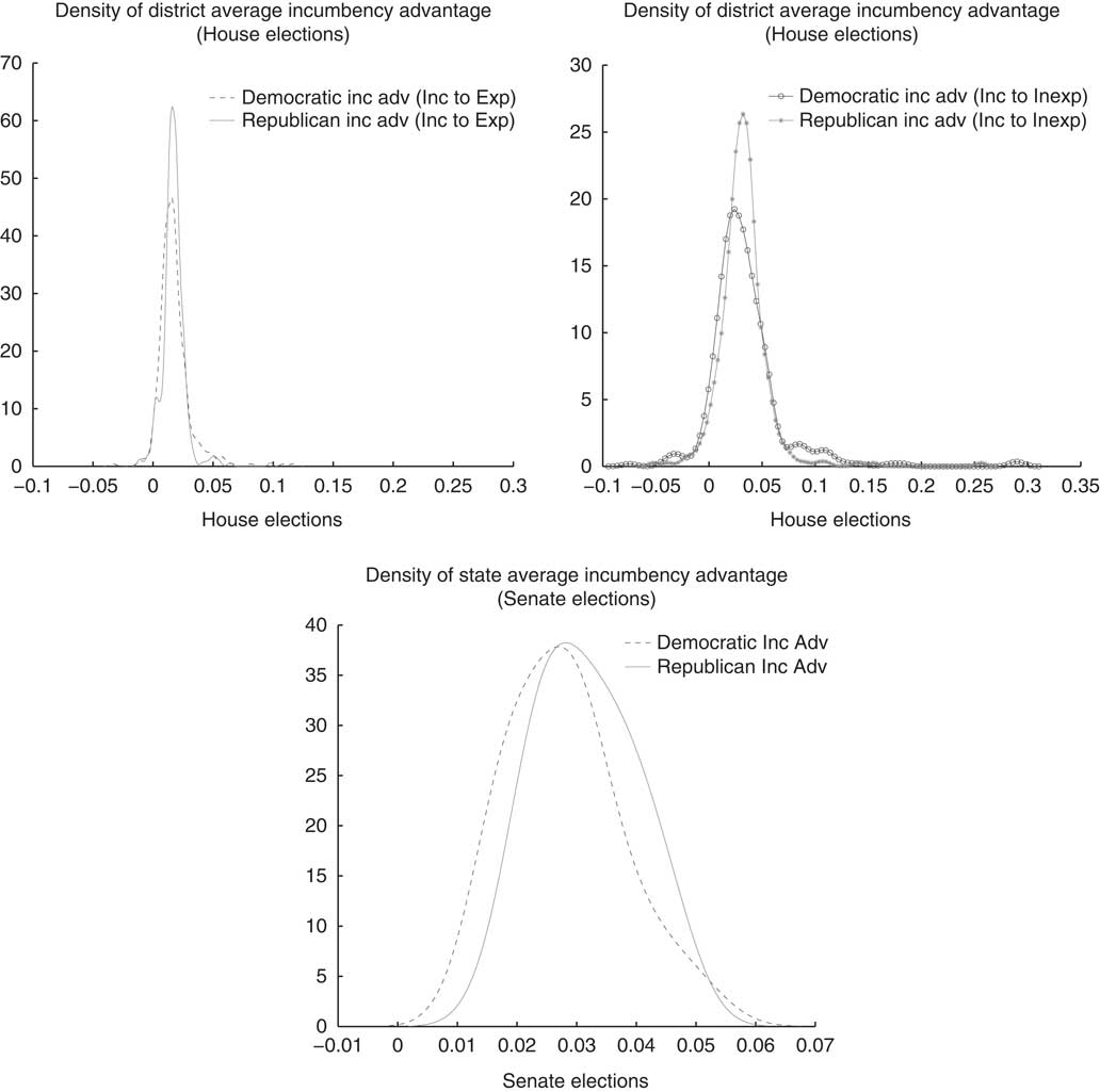
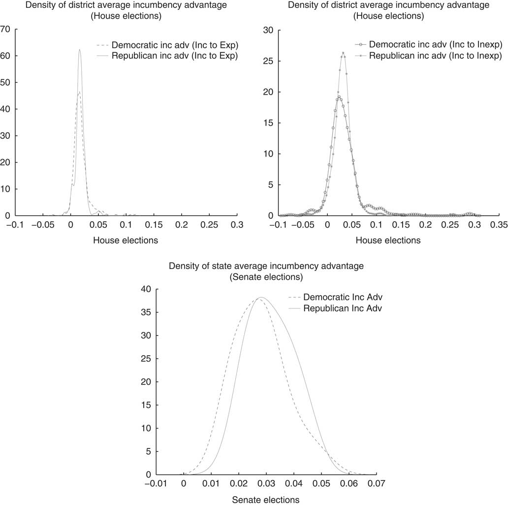
Most empirical research on incumbency advantage is concerned with estimating an average incumbency effect. The theoretical framework shows that incumbency advantage can differ dramatically depending on the distribution of preferences within a district. Figure 2 plots the density of incumbency advantage in the House relative to experienced and inexperienced challengers and in the Senate. The density plots reveal significant cross-district variation in the magnitude of incumbency advantage. For the incumbency advantage relative to inexperienced challengers in the House, there are a handful of districts in which the incumbency advantage is very close to 0 or even negative, the mode is around 0.04, and there are a small number of districts with values above 0.06. The plot is quite similar relative to experienced challengers, but the mode is shifted to the left and there is less dispersion. The incumbency advantage density in the Senate is similar, but displays an even tighter density without the extreme values present in the House districts.
Density function of district average incumbency advantage for Democratic and Republican incumbents in House and Senate elections
While the presence of cross-district variation in incumbency advantage has received little attention in the past, the relationship of the incumbency advantage to districts’ political characteristics is more interesting to observers of American electoral politics. Specifically, I investigate how the ideological predispositions of districts affect the magnitude of incumbency advantage. In moderate districts where large portions of the electorate have ideal policies that are located in the interior of the parties’ positions, an incumbent is able to stake out a location closer to the moderate electorate. In contrast, a challenger with the exact same individual location is perceived as being closer to their relatively extreme party. The signaling value of incumbency is generally less important in extreme districts.Footnote 52
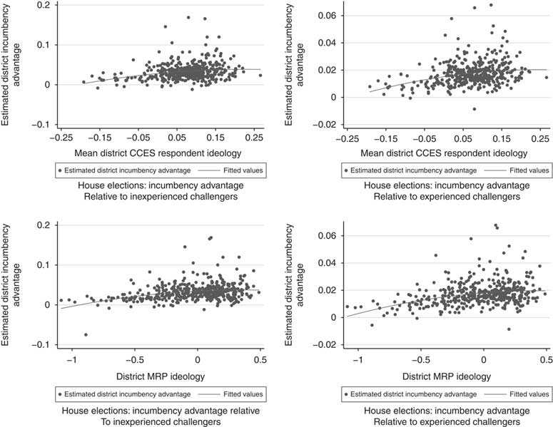
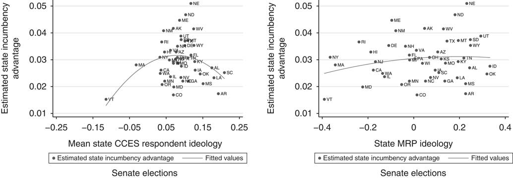
This intuition suggests that the incumbency advantage will be greater in moderate districts and lower in more extreme districts. The exact value of the incumbency advantage will vary subtly with the location of the candidates, parties, voters and individual voter characteristics. To examine how incumbency advantage varies empirically as a function of district ideology, I regress the district estimated incumbency advantage on two measures of district ideology.Footnote 53 The first measure is the mean CCES respondent ideology self-placement for each district and state. The second measure of district and state preferences is the multilevel regression with post-stratification derived from public opinion surveys developed by Tausanovitch and Warshaw.Footnote 54
Figure 3 displays plots of the incumbency advantage relative to both experienced and inexperienced challengers against the CCES mean district ideology and Tausanovitch and Warshaw’sFootnote 55 MRP ideology estimate in the House. Figure 4 reports the plots for the Senate. The estimated incumbency advantage displays a suggestive quadratic relationship in which incumbency advantage is maximized in the most moderate districts. While the relationship between estimated incumbency advantage and district ideology is less precisely estimated in Senate contests due to the small sample size, there is still a statistically significant quadratic relationship for the CCES measure of state ideology.
Scatter plots and quadratic fits

Scatter plots and quadratic fits

The results are consistent with Ashworth and Bueno de Mesquita’sFootnote 56 theoretical predictions and Hirano and Snyder’sFootnote 57 empirical finding that the incumbency advantage is greater in more competitive electoral districts. Hirano and SnyderFootnote 58 attribute some of the overall increase in incumbency advantage to higher direct officeholder benefits in competitive districts. The mechanism here is instead based on cross-district differences in the electoral value of the ability to distinguish a candidate’s ideological location from that of the party.
PARTY POLARIZATION’S EFFECT ON INCUMBENCY ADVANTAGE
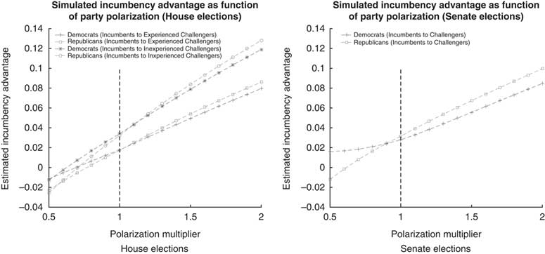
One advantage of specifying a complete individual-level model is that it allows me to investigate the effect of out-of-sample changes on incumbency advantage. While there are many potential applications, I briefly focus on the effect of interparty polarization on incumbency advantage. The framework suggests that increases in polarization amplify the obstacles for challengers, particularly those attempting to win seats in moderate districts. When challengers compete in ideologically moderate or opposed districts, they are burdened by the relatively extreme ideological labels of the parties they are affiliated with. While a challenger may attempt to convey that they are ideologically proximate to the district median, this is difficult to do because of the high party ideological weight that voters place on challengers. Increasing polarization typically exacerbates this problem for challengers because it takes the challenger’s party even further from the district median. In contrast, increased polarization can be beneficial to incumbents, because the party weights that voters place on them are smaller. The ideological information conveyed through incumbency is more valuable to candidates in the increased polarization scenario. While most of the normative literature on polarization focuses on its consequences for gridlock and policy making within the legislature,Footnote 59 the perspective advanced here illustrates that polarization can also have the effect of further entrenching incumbents.
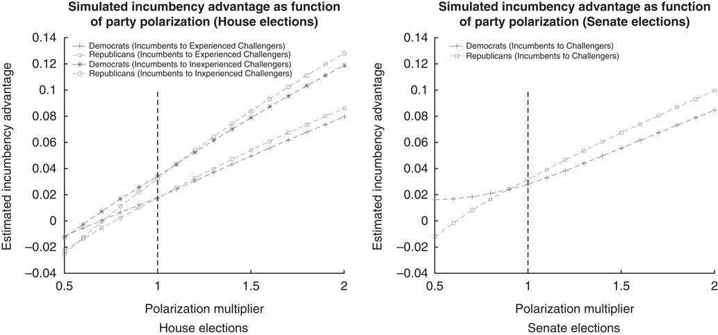
The theoretical framework and parameter estimates allow me to quantify how hypothetical changes in polarization would affect the incumbency advantage. To accomplish this, I simply scale individual CCES respondents’ estimates of each party’s ideological location using a polarization multiplier. I then use the estimated coefficients from the full model reported in Column 4 of Tables 3 and 4 to compute the legislature-wide incumbency advantage for the given polarization multiplier. I repeat this procedure for all polarization multipliers between 0.5 and 2, inclusive, in increments of 0.1.
Figure 5 reports the simulated incumbency advantage for alternative party polarization scenarios in the House and Senate. As the figure makes clear, the incumbency advantage increases with party polarization in both House and Senate elections. However, the slope of this effect is significantly steeper in the House than in the Senate. This finding is consistent with the result that informational effects are larger in the House than in the Senate. Moreover, party polarization has a much greater effect on the incumbency advantage defined by transforming incumbents to inexperienced challengers relative to the incumbency advantage defined by moving incumbents to experienced challengers. This is also consistent with the informational advantage that experienced challengers have relative to inexperienced challengers in House elections. The results also allow the direct examination of out-of-sample counterfactuals. The figures illustrate that reducing citizens’ perceptions of party polarization by 50 per cent would essentially eliminate the incumbency advantage in the House and Senate. Increasing party polarization by 50 per cent would increase the incumbency advantage from approximately 2 per cent to 5 per cent in the House, and from approximately 2.8 to 5.6 per cent for Democrats and 3.2 to 6.7 for Republicans in the Senate.Footnote 60 These are large percentage-point increases that illustrate how further increases in polarization may not only affect internal legislative policy making, but may also spill over into the electoral arena.
Simulated incumbency advantage as a function of party polarization Note: party polarization is increased or decreased by multiplying each respondent’s estimate of the parties’ ideological location by a polarization multiplier. The dashed vertical line represents a polarization multiplier of 1, which is equivalent to the observed incumbency advantage in the sample. The models are estimated with the parameters from the full model, which include both district- or state-fixed effects and individual respondent demographic covariates.
ROBUSTNESS
In the online appendix, I implement a number of robustness checks. Across the robustness checks there are relatively minor changes to the point estimates and standard errors of the coefficient and incumbency advantage estimates. First, I re-estimate the model using the restricted sample of House elections before 2012 to address concerns that the results are contaminated by redistricting between the 2010 and 2012 electoral cycles.
Secondly, I account for the differences in how the CCES solicits ideological information between the 2006 and 2008 waves and the 2010 and 2012 waves of the survey. As mentioned above, I use ideological responses on a 0–100 point scale from the 2006 and 2008 CCES and a seven-point scale from the 2010 and 2012 waves. While I standardize all ideology responses to a scale of −0.5 to 0.5, there is still a potential that the finer grid available for ideology estimates in 2006 and 2008 is affecting the results. To alleviate this concern, I round all of the 2006 and 2008 ideology responses to their corresponding values on a seven-point interval between −0.5 and 0.5 and re-estimate the models with the transformed ideology scores.
Thirdly, I impute missing values of candidate estimates by taking the average report from voters in the same election district. Many of the respondents in the CCES refrain from reporting an estimate of the congressional candidate’s ideological location. In the base specification, these respondents are removed from the estimation sample. If the removed respondents have systematically different parameters than the included respondents, then the parameter estimates will be biased. To investigate the possible extent of this bias, I include omitted respondents by imputing the missing candidate locations using the average district estimate.
Fourthly, I weight the results by the case weights used in the CCES. The CCES oversamples certain subpopulations, such as likely voters. To accommodate the possibility that the unweighted results generate biased parameter estimates, I weight the likelihood function and estimate the parameters with this weighted likelihood function.
Fifthly, I include the respondents’ self-reported partisanship as additional covariates in the vote choice equation. I use respondents’ three-point partisan identification and include self-reported Democrats and Republicans as two additional indicator variables in the regression equation to allow the probability of voting for the Democratic congressional candidate to vary across self-reported Democrats and Republicans.Footnote 61 A concern with this approach is that some of the variation in self-reported partisanship may be due to respondents’ ideology and, as a result, the estimated effect of partisanship will include some of the effect of ideology. Absent a credible research design to disentangle the effects of individual ideology and partisanship on vote choice, these results should be interpreted with caution. Unsurprisingly, the coefficient estimate on Democratic partisanship is positive and the coefficient estimate on Republican partisanship is negative. More interestingly, the ordering of the party weights is preserved and the magnitudes are statistically distinguishable from one another in the case of House elections. With the inclusion of these partisan identity covariates, the overall pattern of results is very similar to the base specification.
CONCLUSION
I have developed and estimated a model of voter learning about candidate ideology that generates an incumbency advantage. The empirical analysis shows that voters in House elections believe incumbents are located closer to the candidates’ individual ideological positions, while challengers are closer to the positions of their parties. However, the difference between incumbents and challengers is substantively and statistically insignificant in Senate elections. The parameter estimates generate an incumbency advantage due to incumbents’ ability to signal ideological positions that are distinct from those of their parties. I decompose the incumbency advantage into its valence and ideological signaling components and find that the signaling component is larger in House elections than Senate elections. Using the estimated parameters from the individual-level voter model, I find that the magnitude of the incumbency advantage systematically varies with the ideological characteristics of the districts and is highest in moderate districts. I also find that increases in the level of partisan polarization would increase the magnitude of the incumbency advantage.
The results have important implications for the measurement of incumbency advantage, voter processing of partisan ideological information and the design of electoral institutions in the presence of electorally entrenched incumbents. The individual-level estimates of the magnitude of the incumbency advantage are similar to estimates in previous research using aggregate election returns. Unlike most prior empirical research, which has focused on estimating a legislature-wide incumbency advantage, the individual-level estimates naturally allow me to examine how incumbency advantage varies across districts. I find suggestive evidence that the incumbency advantage is higher in moderate districts, where the ideological signaling mechanism is most valuable to candidates. While previous research has emphasized the importance of partisan information in citizens’ evaluations of candidates’ ideology, I find that there is an interaction between party ideological information and candidate experience in House elections. Incumbents are less beholden to the ideological information contained in their party than experienced and inexperienced challengers. Voters place the greatest party weight on inexperienced challengers. Finally, the analysis illustrates that attempts to level the playing field between incumbents and challengers through the design of electoral institutions depend critically on cross-district differences in the magnitude of the incumbency advantage.