1 Introduction
When acoustic waves propagate through a volume of turbulence, the unsteady scattering results in a spatial redistribution of the acoustic energy as well as an alteration of the spectral content of the waves. Such scattering is observed, for example, when tones generated by the turbine stages of a turbofan engine are radiated from the exhaust through the turbulent shear layers developing downstream of the engine. The tonal components of the acoustic spectra measured in the far field tend to be attenuated, and a broadband component is observed around the tones. Similar observations are made when acoustic measurements are carried out in open-jet wind tunnels and microphones are located outside the jet flow. The scattering of sound has also received attention in the domain of atmospheric propagation. Sounding techniques using an emitter and a receiver, associated with models of the scattering by a turbulent atmosphere, have been developed to deduce characteristics of the turbulence (intensity and length scales).
Spectral broadening occurs when the base flow is evolving in time, either because of the convection of the turbulence (relative to the source of the observer) or because of the loss of temporal correlation associated with non-frozen turbulence. This was observed experimentally by Candel, Guédel & Julienne (Reference Candel, Guédel and Julienne1975, Reference Candel, Guédel and Julienne1976a ), Candel, Julliand & Julienne (Reference Candel, Julliand and Julienne1976b ) and Schlinker & Amiet (Reference Schlinker and Amiet1980) in the effect of the turbulent shear layer of an open-jet wind tunnel on acoustic measurements performed outside the jet flow when a time-harmonic source was placed on the jet centreline. The measured spectra displayed a number of characteristic features: the peak at the source frequency was attenuated and surrounded by two sidebands, also called a ‘haystack’. These experiments, as well as more recent measurements by Kröber, Hellmold & Koop (Reference Kröber, Hellmold and Koop2013) and Sijtsma et al. (Reference Sijtsma, Oerlemans, Tibbe, Berkefeld and Spehr2014), investigated the evolution of the sidebands with the source frequency and the jet velocity. Candel et al. (Reference Candel, Guédel and Julienne1975) suggested that the positions of the maxima of the sidebands relative to the peak can be related to a macroscale of the turbulence by a Doppler effect.
Kraichnan (Reference Kraichnan1953) and Lighthill (Reference Lighthill1953) developed the first theoretical models for acoustic scattering by turbulent flows, both using Lighthill’s acoustic analogy. Assuming that the scattering is weak, i.e. the proportion of scattered energy is small, Lighthill’s work focused on the description of spatial scattering while Kraichnan also derived expressions for the acoustic spectrum scattered by isotropic turbulence. Howe (Reference Howe1973) developed a set of kinematic equations, in which the different terms can be related to either spatial or spectral scattering. This model included the effect of multiple scattering which can appear if the turbulent volume is large enough so that acoustic waves are scattered successively by numerous eddies, while previous models were restricted to the hypothesis of single scattering (usually using the Born approximation). Brown (Reference Brown1974) and Brown & Clifford (Reference Brown and Clifford1973, Reference Brown and Clifford1976) developed an analytical model for the scattered intensity based on an inhomogeneous Helmholtz equation with a source term involving velocity and temperature fluctuations. The parabolic equation has been used to derive both analytical (Ostashev et al.
Reference Ostashev, Salomons, Clifford, Lataitis, Wilson, Blanc-Benon and Juvé2001) and numerical (Dallois, Blanc-Benon & Juvé Reference Dallois, Blanc-Benon and Juvé2001) models for the evolution of the sound pressure level with the propagation distance through turbulence. Most of the semianalytical and numerical models found in the literature rely on the use of a stochastic method to describe the turbulent field. Goedecke et al. (Reference Goedecke, Wood, Auvermann, Ostashev, Havelock and Ting2001) start from the calculation of the scattering by a single eddy convected in a mean wind. This is then coupled to a discretisation of the turbulent volume in a collection of cells, each containing an eddy. Wilson et al. (Reference Wilson, Ostashev, Goedecke and Auvermann2004) apply a similar method, but use a quasiwavelet method to describe a stationary turbulent velocity field over a barrier and estimate the sound field scattered behind the barrier. Stochastic methods based on a sum of spatial Fourier modes have also been used, for example by Karweit et al. (Reference Karweit, Blanc-Benon, Juvé and Comte-Bellot1991), with a ray tracing technique to study the phase variance of acoustic waves propagating through turbulence, or by Cheinet et al. (Reference Cheinet, Ehrhardt, Juvé and Blanc-Benon2012) and Ehrhardt et al. (Reference Ehrhardt, Cheinet, Juvé and Blanc-Benon2013), combined with a finite-difference time-domain method for the propagation of sound. The scattering by a region of turbulent temperature fluctuations has been investigated by Hargreaves, Kendrick & von Hünerbein (Reference Hargreaves, Kendrick and von Hünerbein2014) using a
 $k$
-space numerical model. Campos (Reference Campos1978a
,Reference Campos
b
) developed an analytical model and derived low- and high-frequency approximations for the scattering by a shear layer. Applications of this model to the data from Candel et al. (Reference Candel, Guédel and Julienne1975) showed good predictions of the overall trends followed by the sidebands. Other models developed for similar configurations include the work of Guédel (Reference Guédel1985), based on Lighthill’s analogy with a low-frequency assumption, and the work of Powles, Tester & McAlpine (Reference Powles, Tester and McAlpine2011) and McAlpine, Powles & Tester (Reference McAlpine, Powles and Tester2013) using high-frequency asymptotics and a weak scattering assumption.
The first attempts at numerical simulations were reported by Ewert et al. (Reference Ewert, Kornow, Tester, Powles, Delfs and Rose2008, Reference Ewert, Kornow, Delfs, Yin, Röber and Rose2009), who solved the linearised Euler equations together with a stochastic method to synthesise the turbulence in a shear layer. Despite issues in the choice of parameters, the method showed promising results in its ability to recover features of the spectral broadening. Recently, a large eddy simulation of the scattering by a mixing layer was carried out by Bennaceur et al. (Reference Bennaceur, Mincu, Mary, Terracol, Larchevêque and Dupont2016). The results were compared against available experimental data with similar non-dimensional scattering parameters and good agreement was found for the shape and position of the sidebands.
On the one hand, previous theoretical studies of spectral broadening had to apply a number of simplifications, such as the Born approximation for the scattering. As a result, the detailed properties of the scattered field were lost, and often not discussed in any detail. On the other hand, while numerical simulations of the scattering by a shear layer have the advantage of providing a complete description of the physical problem and the results are more directly comparable to experimental data, these simulations combine a large number of different physical processes (scattering by individual vortices of varying sizes, convection and sweeping of these vortices, refraction by the mean shear layer, turbulence noise, etc. …) which make it difficult to identify precisely the mechanisms responsible for the spectral broadening.
The present work considers a simplified two-dimensional situation with a single vortex scattering a given sound field to provide further details on scattering by turbulence. The characteristic shape of the sidebands observed on the acoustic spectra as well as the effects of various parameters can be explained by the directivity of the scattered field combined with the different Doppler shifts due to the relative motions of the source, vortex and observer.
Two different models are used for this purpose. First, a semianalytical method is presented in § 2 to study the scattering of plane waves by a steady vortex. It is based on the linearised Euler equations solved in the frequency domain for a plane wave scattered by a steady vortex. No simplification is made regarding the sound frequency or the size and strength of the vortex. This model is relatively fast and allows for a thorough parametric study of the scattered field. For instance, the transition and radical changes in the scattering between the low- and high-frequency domains are described in detail.
For a steady vortex, only spatial scattering is observed, and spectral broadening is only observed when the vortex is moving relative to the source or observer. The seminumerical method is therefore extended in § 3 to account for the Doppler shifts due to the relative motion between the vortex and the observer. The resulting acoustic spectra display sidebands around a peak at the source frequency, presenting similarities with the sidebands observed in experimental studies of the scattering by a turbulent shear layer. The analysis of the model shows that the shape and position of the sidebands are directly explained by the directivity of the scattered field from the vortex, associated with a Doppler effect due to the motion of the vortex. The dependence of the spectra on the source frequency and convection velocity is also consistent with previous observations of haystacking.
In addition, a fully numerical method is used to consider more general incident sound fields, since the first model is limited to plane waves. It also relies on the linearised Euler equations, but solved in the time domain with a finite-difference approach. It provides verification results for the first model in §§ 2 and 3. Then, in § 4, it is used to consider the scattering of the sound field radiated by a fixed point source. This test case completes the description of the Doppler effects involved in the spectral broadening, in particular due to the motion of the vortex relative to the source.
2 Sound scattering by a steady vortex
Before discussing the spectral broadening induced by moving vortices (see § 3) it is necessary to describe in detail the sound scattering by a steady vortex. A number of authors have treated this problem analytically under the low-frequency limit, such as Ferziger (Reference Ferziger1974), Howe (Reference Howe1975), O’Shea (Reference O’Shea1975), Colonius, Lele & Moin (Reference Colonius, Lele and Moin1994) or more recently Ford & Llewellyn Smith (Reference Ford and Llewellyn Smith1999) and Llewellyn Smith & Ford (Reference Llewellyn Smith and Ford2001a ,Reference Llewellyn Smith and Ford b ) using matched asymptotic expansions. For high frequencies, Georges (Reference Georges1972) suggested the use of a ray tracing technique to determine the ray paths and Colonius et al. (Reference Colonius, Lele and Moin1994) extended this approach by calculating the amplitudes and phases of the waves. Candel (Reference Candel1979) used a parabolic approximation to perform computations of the scattering of plane waves by cylindrical inhomogeneities of the refraction index, such as a vortex core. Direct numerical simulations were performed by Colonius et al. (Reference Colonius, Lele and Moin1994) in two dimensions and later by Hattori & Llewellyn Smith (Reference Hattori and Llewellyn Smith2002) in three dimensions, again for relatively low frequencies of the incident waves relative to the vortex core dimension. This section presents two models and a parametric study to provide a thorough discussion of the scattering by a steady vortex in two dimensions. These models do not rely on approximations for either low or high frequencies, or for weak vortices (i.e. small values of the Mach number based on the maximum of the vortex velocity).
The propagation and refraction of small-amplitude acoustic waves through a vortex can be described by the linearised Euler equations (LEEs), written here in non-conservative form for isentropic perturbations,
 $$\begin{eqnarray}\left.\begin{array}{@{}c@{}}{\displaystyle \frac{\unicode[STIX]{x2202}\unicode[STIX]{x1D70C}^{\prime }}{\unicode[STIX]{x2202}t}}+\boldsymbol{u}\boldsymbol{\cdot }\unicode[STIX]{x1D735}\unicode[STIX]{x1D70C}^{\prime }+\boldsymbol{u}^{\prime }\boldsymbol{\cdot }\unicode[STIX]{x1D735}\unicode[STIX]{x1D70C}+\unicode[STIX]{x1D70C}\unicode[STIX]{x1D735}\boldsymbol{\cdot }\boldsymbol{u}^{\prime }+\unicode[STIX]{x1D70C}^{\prime }\unicode[STIX]{x1D735}\boldsymbol{\cdot }\boldsymbol{u}=0,\\ {\displaystyle \frac{\unicode[STIX]{x2202}\boldsymbol{u}^{\prime }}{\unicode[STIX]{x2202}t}}+(\boldsymbol{u}\boldsymbol{\cdot }\unicode[STIX]{x1D735})\boldsymbol{u}^{\prime }+(\boldsymbol{u}^{\prime }\boldsymbol{\cdot }\unicode[STIX]{x1D735})\boldsymbol{u}+{\displaystyle \frac{\unicode[STIX]{x1D735}p^{\prime }}{\unicode[STIX]{x1D70C}}}-\unicode[STIX]{x1D70C}^{\prime }{\displaystyle \frac{\unicode[STIX]{x1D735}p}{\unicode[STIX]{x1D70C}^{2}}}=\mathbf{0},\\ {\displaystyle \frac{\unicode[STIX]{x2202}p^{\prime }}{\unicode[STIX]{x2202}t}}+\boldsymbol{u}\boldsymbol{\cdot }\unicode[STIX]{x1D735}p^{\prime }+\boldsymbol{u}^{\prime }\boldsymbol{\cdot }\unicode[STIX]{x1D735}p+\unicode[STIX]{x1D6FE}p\unicode[STIX]{x1D735}\boldsymbol{\cdot }\boldsymbol{u}^{\prime }+\unicode[STIX]{x1D6FE}p^{\prime }\unicode[STIX]{x1D735}\boldsymbol{\cdot }\boldsymbol{u}=0,\end{array}\right\}\end{eqnarray}$$
where
 $\unicode[STIX]{x1D70C}$
,
 $\boldsymbol{u}$
and
 $p$
denote the base flow properties, and the acoustic fluctuations are
 $\unicode[STIX]{x1D70C}^{\prime }$
,
 $\boldsymbol{u}^{\prime }$
and
 $p^{\prime }$
;
 $\unicode[STIX]{x1D6FE}$
is the heat capacity ratio.
In this paper, following Colonius et al. (Reference Colonius, Lele and Moin1994), an inviscid vortex with zero circulation is considered. The following expressions for the velocity, pressure and density in the base flow are solutions of the Euler equations (using polar coordinates
 $r$
and
 $\unicode[STIX]{x1D703}$
centred on the vortex):
 $$\begin{eqnarray}\left.\begin{array}{@{}c@{}}\boldsymbol{u}(r)=U_{v}{\displaystyle \frac{r}{L}}\exp \left[{\displaystyle \frac{1}{2}}(1-r^{2}/L^{2})\right]\boldsymbol{e}_{\unicode[STIX]{x1D703}},\\ p(r)=p_{\infty }\left[1-{\displaystyle \frac{\unicode[STIX]{x1D6FE}-1}{2}}M_{v}^{2}\exp (1-r^{2}/L^{2})\right]^{\unicode[STIX]{x1D6FE}/(\unicode[STIX]{x1D6FE}-1)},\\ \unicode[STIX]{x1D70C}(r)=\unicode[STIX]{x1D70C}_{\infty }[p(r)/p_{\infty }]^{1/\unicode[STIX]{x1D6FE}},\end{array}\right\}\end{eqnarray}$$
where
 $\unicode[STIX]{x1D70C}_{\infty }$
,
 $p_{\infty }$
and
 $c_{\infty }$
are the density, pressure and sound speed in the fluid at rest, related by
 $\unicode[STIX]{x1D70C}_{\infty }c_{\infty }^{2}=\unicode[STIX]{x1D6FE}p_{\infty }$
. The unit vectors of the cylindrical coordinates are denoted by
 $(\boldsymbol{e}_{r},\boldsymbol{e}_{\unicode[STIX]{x1D703}})$
. The vortex is characterised by its maximum velocity
 $U_{v}$
and its core size
 $L$
, so that
 $u_{\unicode[STIX]{x1D703}}(r=L)=U_{v}$
. We also define the associated Mach number of the vortex
 $M_{v}=U_{v}/c_{\infty }$
.
2.1 Numerical model
The LEEs (2.1) are solved in the time domain using a high-order finite-difference method. Spatial derivatives are approximated using seven-point fourth-order dispersion-relation-preserving (DRP) stencils (Tam Reference Tam2012). An explicit eighth-order filter is applied to damp high-frequency spurious oscillations. The time integration is performed using the standard fourth-order Runge–Kutta scheme. Cartesian grids are used throughout this work. Outgoing waves are absorbed by buffer zones with artificial damping around the domain. One-dimensional characteristic boundary conditions are applied on the last grid points (Thompson Reference Thompson1987). Tam & Dong (Reference Tam and Dong1996) radiation and outflow boundary conditions are also available. The incident sound field (either a plane wave or the sound generated by a mass source) is introduced in the simulation through a relaxation term in the buffer zones. These numerical schemes are implemented in the PIANO solver developed by Deutsches zentrum für Luft- und Raumfahrt (DLR) (Ewert et al. Reference Ewert, Kornow, Tester, Powles, Delfs and Rose2008, Reference Ewert, Kornow, Delfs, Yin, Röber and Rose2009) and used in this work.
2.2 Semianalytical model
The starting point is the LEEs (2.1), written in cylindrical coordinates using vector notation,
 $$\begin{eqnarray}\frac{\unicode[STIX]{x2202}\boldsymbol{q}^{\prime }}{\unicode[STIX]{x2202}t}+\unicode[STIX]{x1D63C}\boldsymbol{q}^{\prime }+\unicode[STIX]{x1D63D}\frac{\unicode[STIX]{x2202}\boldsymbol{q}^{\prime }}{\unicode[STIX]{x2202}r}+\unicode[STIX]{x1D63E}\frac{1}{r}\frac{\unicode[STIX]{x2202}\boldsymbol{q}^{\prime }}{\unicode[STIX]{x2202}\unicode[STIX]{x1D703}}=\mathbf{0},\end{eqnarray}$$
where
 $\boldsymbol{q}^{\prime }=(\unicode[STIX]{x1D70C}^{\prime },\boldsymbol{u}^{\prime },p^{\prime })^{\text{T}}$
and
 $$\begin{eqnarray}\left.\begin{array}{@{}c@{}}\unicode[STIX]{x1D63C}=\left[\begin{array}{@{}cccc@{}}0 & {\displaystyle \frac{\unicode[STIX]{x1D70C}}{r}}+{\displaystyle \frac{\text{d}\unicode[STIX]{x1D70C}}{\text{d}r}} & 0 & 0\\ {\displaystyle \frac{-u_{\unicode[STIX]{x1D703}}^{2}}{\unicode[STIX]{x1D70C}r}} & 0 & {\displaystyle \frac{-2u_{\unicode[STIX]{x1D703}}}{r}} & 0\\ 0 & {\displaystyle \frac{\text{d}u_{\unicode[STIX]{x1D703}}}{\text{d}r}}+{\displaystyle \frac{u_{\unicode[STIX]{x1D703}}}{r}} & 0 & 0\\ 0 & {\displaystyle \frac{\unicode[STIX]{x1D6FE}p}{r}}+{\displaystyle \frac{\text{d}p}{\text{d}r}} & 0 & 0\end{array}\right],\quad \unicode[STIX]{x1D63D}=\left[\begin{array}{@{}cccc@{}}0 & \unicode[STIX]{x1D70C} & 0 & 0\\ 0 & 0 & 0 & {\displaystyle \frac{1}{\unicode[STIX]{x1D70C}}}\\ 0 & 0 & 0 & 0\\ 0 & \unicode[STIX]{x1D6FE}p & 0 & 0\end{array}\right],\\ \unicode[STIX]{x1D63E}=\left[\begin{array}{@{}cccc@{}}u_{\unicode[STIX]{x1D703}} & 0 & \unicode[STIX]{x1D70C} & 0\\ 0 & u_{\unicode[STIX]{x1D703}} & 0 & 0\\ 0 & 0 & u_{\unicode[STIX]{x1D703}} & {\displaystyle \frac{1}{\unicode[STIX]{x1D70C}}}\\ 0 & 0 & \unicode[STIX]{x1D6FE}p & u_{\unicode[STIX]{x1D703}}\end{array}\right].\end{array}\right\}\end{eqnarray}$$
It should be noted that the expressions for the coefficient matrices
 $\unicode[STIX]{x1D63C}$
,
 $\unicode[STIX]{x1D63D}$
and
 $\unicode[STIX]{x1D63E}$
have been simplified assuming that the base flow is independent of
 $\unicode[STIX]{x1D703}$
and has no radial velocity component.
The fluctuations
 $\boldsymbol{q}^{\prime }$
are written as the sum of a given incident field
 $\boldsymbol{q}_{i}^{\prime }=(\unicode[STIX]{x1D70C}_{i}^{\prime },\boldsymbol{u}_{i}^{\prime },p_{i}^{\prime })^{\text{T}}$
and a scattered field
 $\boldsymbol{q}_{s}^{\prime }=(\unicode[STIX]{x1D70C}_{s}^{\prime },\boldsymbol{u}_{s}^{\prime },p_{s}^{\prime })^{\text{T}}$
. Both are assumed to be time-harmonic with angular frequency
 $\unicode[STIX]{x1D714}$
and are decomposed into azimuthal components using a Fourier series in
 $\unicode[STIX]{x1D703}$
,
 $$\begin{eqnarray}\boldsymbol{q}_{i}^{\prime }(r,\unicode[STIX]{x1D703},t)=\mathop{\sum }_{m=-\infty }^{+\infty }\boldsymbol{q}_{i,m}^{\prime }(r)\text{e}^{\text{i}\unicode[STIX]{x1D714}t-\text{i}m\unicode[STIX]{x1D703}},\quad \boldsymbol{q}_{s}^{\prime }(r,\unicode[STIX]{x1D703},t)=\mathop{\sum }_{m=-\infty }^{+\infty }\boldsymbol{q}_{s,m}^{\prime }(r)\text{e}^{\text{i}\unicode[STIX]{x1D714}t-\text{i}m\unicode[STIX]{x1D703}}.\end{eqnarray}$$
Since the base flow is axisymmetric, the equation for each azimuthal order
 $m$
is decoupled from the other orders. For azimuthal order
 $m$
, the LEEs (2.1) yield
 $$\begin{eqnarray}\text{i}\unicode[STIX]{x1D714}\boldsymbol{q}_{s,m}^{\prime }+\unicode[STIX]{x1D63C}\boldsymbol{q}_{s,m}^{\prime }+\unicode[STIX]{x1D63D}\frac{\text{d}\boldsymbol{q}_{s,m}^{\prime }}{\text{d}r}-\frac{\text{i}m}{r}\unicode[STIX]{x1D63E}\boldsymbol{q}_{s,m}^{\prime }=-\text{i}\unicode[STIX]{x1D714}\boldsymbol{q}_{i,m}^{\prime }-\unicode[STIX]{x1D63C}\boldsymbol{q}_{i,m}^{\prime }-\unicode[STIX]{x1D63D}\frac{\text{d}\boldsymbol{q}_{i,m}^{\prime }}{\text{d}r}+\frac{\text{i}m}{r}\unicode[STIX]{x1D63E}\boldsymbol{q}_{i,m}^{\prime }.\end{eqnarray}$$
These ordinary differential equations are readily solved using a finite-difference approximation for the radial derivative. Here, we use a seven-point fourth-order DRP scheme on a uniform grid. The grid points are denoted by
 $r_{n}$
, with
 $n=1,\ldots ,N$
, and the grid spacing by
 $\unicode[STIX]{x0394}r$
.
Parity conditions should be satisfied at
 $r=0$
to ensure the regularity of the solution formulated in cylindrical coordinates (Lewis & Bellan Reference Lewis and Bellan1990; Boyd Reference Boyd2001). Here, we use a technique similar to that of Mohseni & Colonius (Reference Mohseni and Colonius2000), where three ghost points are defined with negative
 $r$
coordinates. They are mirror images of the first three physical points (
 $r_{1-l}=-r_{l}$
, with
 $l=1$
,
 $2$
and
 $3$
). By setting
 $r_{1}=-r_{0}=\unicode[STIX]{x0394}r/2$
, the singularity in the governing equations at
 $r=0$
lies between two grid points. The equations used for the ghost points are directly provided by the symmetry conditions for scalar fields of the form (2.5),
 $$\begin{eqnarray}\unicode[STIX]{x1D70C}^{\prime }(-r)=\unicode[STIX]{x1D70C}^{\prime }(r)\text{e}^{-\text{i}m\unicode[STIX]{x03C0}},\quad p^{\prime }(-r)=p^{\prime }(r)\text{e}^{-\text{i}m\unicode[STIX]{x03C0}},\end{eqnarray}$$
and for vector fields,
 $$\begin{eqnarray}u_{r}^{\prime }(-r)=-u_{r}^{\prime }(r)\text{e}^{-\text{i}m\unicode[STIX]{x03C0}},\quad u_{\unicode[STIX]{x1D703}}^{\prime }(-r)=-u_{\unicode[STIX]{x1D703}}^{\prime }(r)\text{e}^{-\text{i}m\unicode[STIX]{x03C0}}.\end{eqnarray}$$
This technique yields solutions satisfying the parity conditions specified in Lewis & Bellan (Reference Lewis and Bellan1990).
Beyond some distance
 $R$
away from the vortex, its induced velocity can be considered to be negligible and one is left with sound waves propagating in a uniform medium at rest. It follows that for
 $r>R$
one can write the scattered field as a sum of progressive cylindrical waves satisfying the Helmholtz equation. Since the scattered field satisfies the Sommerfeld radiation condition, the solution for a given azimuthal order
 $m$
reads as
 $$\begin{eqnarray}\boldsymbol{q}_{s,m}^{\prime }(r)=A_{m}\left(\begin{array}{@{}c@{}}\mathit{H}_{m}^{(2)}(kr)/c_{\infty }^{2}\\ \text{i}\mathit{H}_{m}^{(2)^{\prime }}(kr)/(\unicode[STIX]{x1D70C}_{\infty }c_{\infty })\\ m\mathit{H}_{m}^{(2)}(kr)/(\unicode[STIX]{x1D70C}_{\infty }\unicode[STIX]{x1D714}r)\\ \mathit{H}_{m}^{(2)}(kr)\end{array}\right),\quad \text{for }r>R,\end{eqnarray}$$
where
 $k=\unicode[STIX]{x1D714}/c_{\infty }$
is the free-field wavenumber and
 $\mathit{H}_{m}^{(2)}$
is the
 $m$
th-order Hankel function of the second kind. The grid is defined such that
 $r_{N}=R$
, and three ghost points are added:
 $r_{N+l}=R+l\unicode[STIX]{x0394}r$
, with
 $l=1$
, 2 and 3. The solution for these ghost points is given by (2.9) and the remaining coefficient
 $A_{m}$
is written as a function of the solution at
 $r_{N}$
by
 $A_{m}=p^{\prime }(r_{N})/\mathit{H}_{m}^{(2)}(kR)$
.
When the observer is in the acoustic far field (
 $kr\rightarrow \infty$
), the multipole expansion (2.9) can be further simplified using the asymptotic expression for the Hankel function (Abramowitz & Stegun Reference Abramowitz and Stegun1964, chap. 9). The scattered field can then be written as
 $$\begin{eqnarray}p_{s}^{\prime }(r,\unicode[STIX]{x1D703},t)=\frac{D(\unicode[STIX]{x1D703})}{\sqrt{r}}\text{e}^{\text{i}\unicode[STIX]{x1D714}(t-r/c_{\infty })},\quad \text{with }D(\unicode[STIX]{x1D703})=\sqrt{\frac{2\text{i}}{k\unicode[STIX]{x03C0}}}\mathop{\sum }_{m=-M}^{M}\text{i}^{m}A_{m}\text{e}^{-\text{i}m\unicode[STIX]{x1D703}}.\end{eqnarray}$$
It should be noted that the sum over the azimuthal orders can be truncated because the coefficients
 $A_{m}$
decay rapidly for large values of
 $|m|$
. For all of the results presented below, convergence with respect to the grid resolution and the number of azimuthal orders included in (2.10) has been verified.
When the incident field is an acoustic plane wave propagating along the
 $x$
direction, the pressure can be written as
 $p_{i}^{\prime }(r,\unicode[STIX]{x1D703},t)=P\text{e}^{\text{i}\unicode[STIX]{x1D714}t-\text{i}kr\cos \unicode[STIX]{x1D703}}$
. Its expansion (2.5) in terms of Fourier components gives
 $$\begin{eqnarray}\boldsymbol{q}_{i,m}^{\prime }(r)=P\text{i}^{-m}\left(\begin{array}{@{}c@{}}\text{J}_{m}(kr)/c_{\infty }^{2}\\ \text{i}\text{J}_{m}^{\prime }(kr)/(\unicode[STIX]{x1D70C}_{\infty }c_{\infty })\\ m\text{J}_{m}(kr)/(\unicode[STIX]{x1D70C}_{\infty }\unicode[STIX]{x1D714}r)\\ \text{J}_{m}(kr)\end{array}\right),\end{eqnarray}$$
where
 $\text{J}_{m}$
is the
 $m$
th-order Bessel function of the first kind.
2.3 Test case
The test case previously considered by Colonius et al. (Reference Colonius, Lele and Moin1994) provides a benchmark to verify the time-domain numerical model and the frequency-domain semianalytical model. It involves the scattering of a time-harmonic plane wave propagating in the positive
 $x$
direction by the steady vortex defined by (2.2). The parameters are made non-dimensional by setting
 $c_{\infty }=1$
,
 $\unicode[STIX]{x1D70C}_{\infty }=1$
and
 $L=1$
. The frequency is given by the Helmholtz numbers
 $kL=\unicode[STIX]{x1D714}L/c_{\infty }=\unicode[STIX]{x03C0}/2$
, corresponding to an acoustic wavelength
 $\unicode[STIX]{x1D706}=c_{\infty }/f=4L$
. The vortex velocity is
 $M_{v}=0.125$
and the amplitude of the incident wave is
 $P=1$
.
For the time-domain numerical model, a uniform Cartesian grid is used with resolution
 $\unicode[STIX]{x0394}x=\unicode[STIX]{x0394}y=L/8$
, providing 16 grid points across the core of the vortex. The physical region of the computational domain is
 $-15L\leqslant x\leqslant 15L$
and
 $-15L\leqslant y\leqslant 15L$
and is surrounded by a buffer zone with 50 grid points. The time step corresponds to a Courant number
 $c_{\infty }\unicode[STIX]{x0394}t/\unicode[STIX]{x0394}x=0.9$
. The simulations are run until the solutions reach a periodic state.
For the semianalytical model, the domain
 $0\leqslant r\leqslant 15$
(thus
 $R=15L$
) is discretised with 150 grid points. Equations (2.6) are solved for every azimuthal order in the range
 $-30\leqslant m\leqslant 30$
.
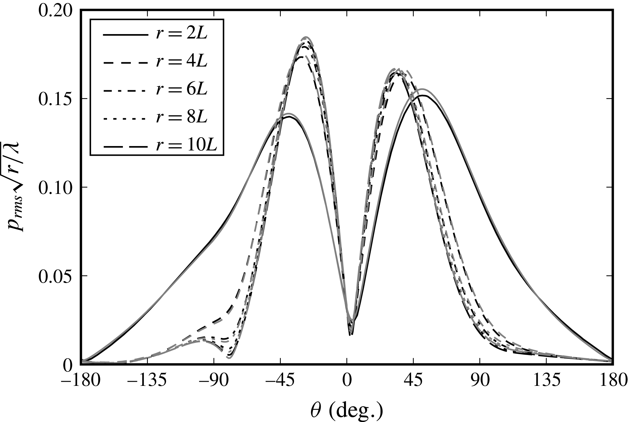
To validate the two models and compare with the results from Colonius et al. (Reference Colonius, Lele and Moin1994), the root-mean-square pressure of the scattered field is plotted in figure 1 as a function of direction for several distances from the vortex from
 $r=\unicode[STIX]{x1D706}_{0}/2$
to
 $r=2.5\unicode[STIX]{x1D706}_{0}$
. The scattered pressure is scaled by
 $\sqrt{r}$
to show that cylindrical spreading is observed away from the vortex. We can see that there is excellent agreement between the two models and the results are also in good agreement with figure 11 in Colonius et al. (Reference Colonius, Lele and Moin1994) (it should be noted that the
 $\unicode[STIX]{x1D703}$
coordinate is reversed since the vortex is spinning in the opposite direction). A similar level of accuracy is observed for the phase of the scattered field. Very good agreement has also been observed for a number of other test cases solved using the two models.
The amplitude of the scattered field (root-mean-squared pressure) at different distances from the vortex and calculated by the time-domain numerical model (black lines) and the frequency-domain model (grey lines). Other parameters are
 $M_{v}=0.125$
and
 $kL=\unicode[STIX]{x03C0}/2$
, corresponding to
 $\unicode[STIX]{x1D706}=4L$
. The results are normalised by the cylindrical spreading
 $1/\sqrt{r}$
and the angle
 $\unicode[STIX]{x1D703}$
is measured from the incident wave direction.

2.4 Spatial scattering
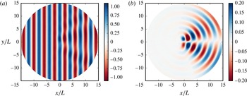
Figure 2 shows examples of the total and scattered fields. In this case, the scattering of the plane wave is relatively mild and there is only a slight alteration of the wave fronts due to the mean flow refraction. As was already visible from figure 1, the scattered field is formed of two beams on either side of the incident wave direction. These beams differ only slightly in direction and amplitude, but they can be seen from figure 2(b) to be out of phase. Their presence can be explained easily by the refraction effect due to the mean flow gradients inside the vortex (see figure 17 in Colonius et al. (Reference Colonius, Lele and Moin1994) for an illustration of this effect in terms of acoustic rays). Figure 1 indicates that there is also a much weaker beam radiated at an angle close to
 $-100^{\circ }$
. However, overall, for these parameters, there is very little sound scattered back in the negative
 $x$
direction.
Snapshots of (a) the total and (b) the scattered pressure fluctuations calculated with the semianalytical model for
 $M_{v}=0.125$
and
 $kL=\unicode[STIX]{x03C0}/2$
.

We will see in § 3 that the properties of haystacking are directly related to the directions and strengths of the scattered beams radiated from a steady vortex. It is therefore important to describe their properties in more detail. The two parameters influencing the spatial scattering by a steady vortex are (i) the ratio between the acoustic wavelength
 $\unicode[STIX]{x1D706}$
and the vortex radius
 $L$
, characterised by the Helmholtz number
 $kL=2\unicode[STIX]{x03C0}L/\unicode[STIX]{x1D706}$
, and (ii) the strength of the vortex, characterised by the Mach number
 $M_{v}$
. These parameters are now studied using the semianalytical model since its speed allows us to perform a detailed parametric study (the time-domain numerical model will be used for the convected vortex and for more complex incident sound fields). All results are shown for
 $\unicode[STIX]{x1D70C}_{\infty }=1$
,
 $c_{\infty }=1$
,
 $L=1$
and
 $P=1$
.
2.4.1 Influence of the Helmholtz number
To assess the influence of the Helmholtz number, it is varied between
 $kL=\unicode[STIX]{x03C0}/5$
and
 $8\unicode[STIX]{x03C0}$
, corresponding to an acoustic wavelength varying between
 $10L$
and
 $L/4$
. For each frequency, the discretisation of the radial direction is chosen to obtain a converged solution. The number of azimuthal orders
 $m$
included in the solution is also adjusted for each frequency and includes
 $-120\leqslant m\leqslant 120$
for the highest frequency. The resulting evolution of the directivity
 $D(\unicode[STIX]{x1D703})$
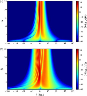
of the scattered field is shown in figure 3 for a relatively weak vortex with
 $M_{v}=0.05$
and for a stronger vortex with
 $M_{v}=0.15$
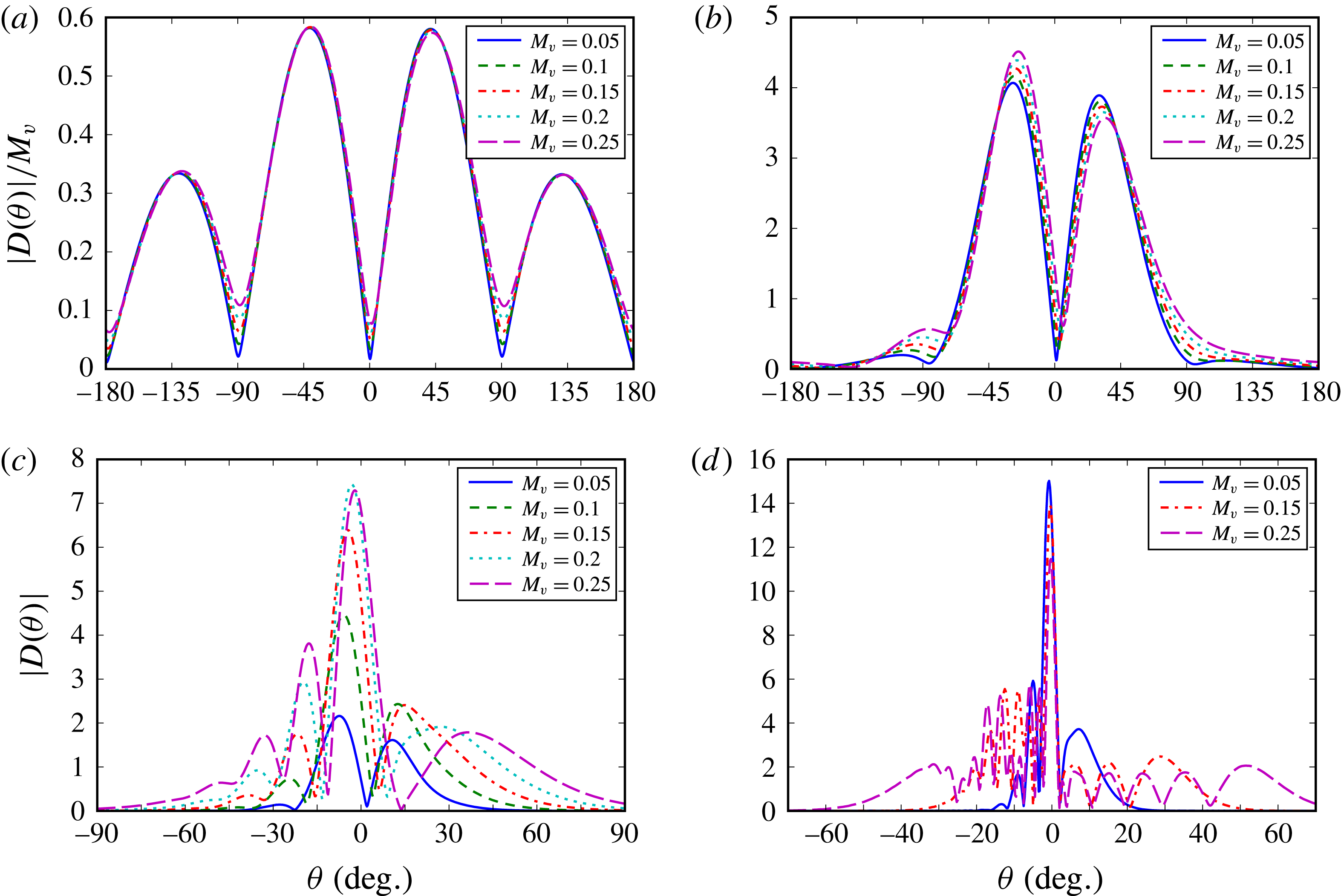
. The influence of the vortex strength is shown at four different frequencies in figure 4, where the directivity
 $D(\unicode[STIX]{x1D703})$
of the scattered field defined in (2.10) is plotted for a range of values of
 $M_{v}$
varying from 0.05 to 0.25.
The directivity
 $D(\unicode[STIX]{x1D703})$
of the scattered pressure in the far field (plotting
 $20\log _{10}(|D|)$
) as a function of the direction
 $\unicode[STIX]{x1D703}$
and the Helmholtz number
 $kL$
with a vortex magnitude of (a)
 $M_{v}=0.05$
and (b)
 $M_{v}=0.15$
. Here,
 $\unicode[STIX]{x1D703}=0^{\circ }$
corresponds to the direction of the incident wave.

The directivity
 $D(\unicode[STIX]{x1D703})$
for four Helmholtz numbers, (a)
 $kL=\unicode[STIX]{x03C0}/5$
, (b)
 $kL=\unicode[STIX]{x03C0}/2$
, (c)
 $kL=2\unicode[STIX]{x03C0}$
and (d)
 $kL=8\unicode[STIX]{x03C0}$
, and for different vortex strengths from
 $M_{v}=0.05$
to 0.25. It should be noted that for (a) and (b) the directivity
 $D(\unicode[STIX]{x1D703})$
is scaled by the vortex Mach number
 $M_{v}$
.

First, we consider low frequencies (
 $kL<1$
), corresponding to a small vortex relative to the acoustic wavelength. Figure 4(a) shows the directivity
 $D(\unicode[STIX]{x1D703})$
scaled by the Mach number
 $M_{v}$
for
 $kL=\unicode[STIX]{x03C0}/5$
. The directivity is symmetric across the direction of the incident wave and similar to that of a lateral quadrupole. The directivity of each scattered beam is well described by a sine function. The magnitude of the scattered field scales like
 $M_{v}$
and is particularly weak compared with higher frequencies. These trends are consistent with the results from analytical models based on low-frequency and low-Mach-number assumptions (O’Shea Reference O’Shea1975; Colonius et al.
Reference Colonius, Lele and Moin1994). These models predict a symmetric scattered field around
 $\unicode[STIX]{x1D703}=0^{\circ }$
and a linear growth of the scattered field with
 $M_{v}$
.
The directivity changes significantly for higher frequencies, as shown in figure 3. The amount of backscattering (
 $|\unicode[STIX]{x1D703}|>90^{\circ }$
) decreases rapidly for higher frequencies and the scattered field is progressively focused closer to the direction of the incident wave. As the frequency increases, there is also a loss of symmetry between the upper and lower parts of the scattered field. The main beam below the
 $x$
axis (
 $\unicode[STIX]{x1D703}<0$
) becomes much stronger than the one above and moves closer to
 $\unicode[STIX]{x1D703}=0$
. In addition, several smaller beams are observed at high frequencies, with more beams developing for
 $\unicode[STIX]{x1D703}<0$
than for
 $\unicode[STIX]{x1D703}>0$
; see, for instance, figure 4(c,d). The strength of the scattered field increases rapidly with frequency, with nearly three orders of magnitude for the maximum value of the scattered field between the lowest and highest frequencies (see figure 4
a,d).
For moderate frequencies,
 $kL\simeq 1$
as in figure 4(b), there are two strong beams similar to those observed in figure 1. The magnitude of the scattered field appears to scale like
 $M_{v}$
, at least qualitatively, but the details are slightly more complex and the asymmetry between the two beams increases for stronger vortices. The difference in amplitude between the two beams increases significantly with
 $M_{v}$
, with the lower beam (
 $\unicode[STIX]{x1D703}<0$
) becoming stronger than the upper beam (
 $\unicode[STIX]{x1D703}>0$
). In addition, the direction of the lower (respectively upper) beam moves closer to (respectively away from) the
 $x$
axis. The presence of asymmetric scattering was already noted by Colonius et al. (Reference Colonius, Lele and Moin1994) in their numerical study and was attributed to the effects of terms with an order in
 $M_{v}$
higher than those retained in their analytical model. While the present model also indicates that the two beams are almost symmetric for small
 $M_{v}$
, it fully captures the effects of the vortex strength on the scattered field for any
 $M_{v}$
.
At higher frequencies,
 $kL>1$
, a number of secondary lobes are visible in the directivity function, especially for
 $\unicode[STIX]{x1D703}<0^{\circ }$
; see figure 3. This trend becomes even more significant for stronger vortices, as can be seen in figure 4(c,d). This results in the scattered field covering a wider angular range than for weak vortices (this is visible when comparing figures 3
a and 3
b). A strong beam starts to dominate from the lower half (
 $\unicode[STIX]{x1D703}<0^{\circ }$
) at midfrequencies and moves towards
 $\unicode[STIX]{x1D703}=0^{\circ }$
as the frequency increases. On the
 $\unicode[STIX]{x1D703}>0^{\circ }$
side, there is a single beam for weak vortices. For high frequencies, the magnitude of the directivity function
 $D(\unicode[STIX]{x1D703})$
does not scale linearly with the vortex strength
 $M_{v}$
; see figure 4(c,d).
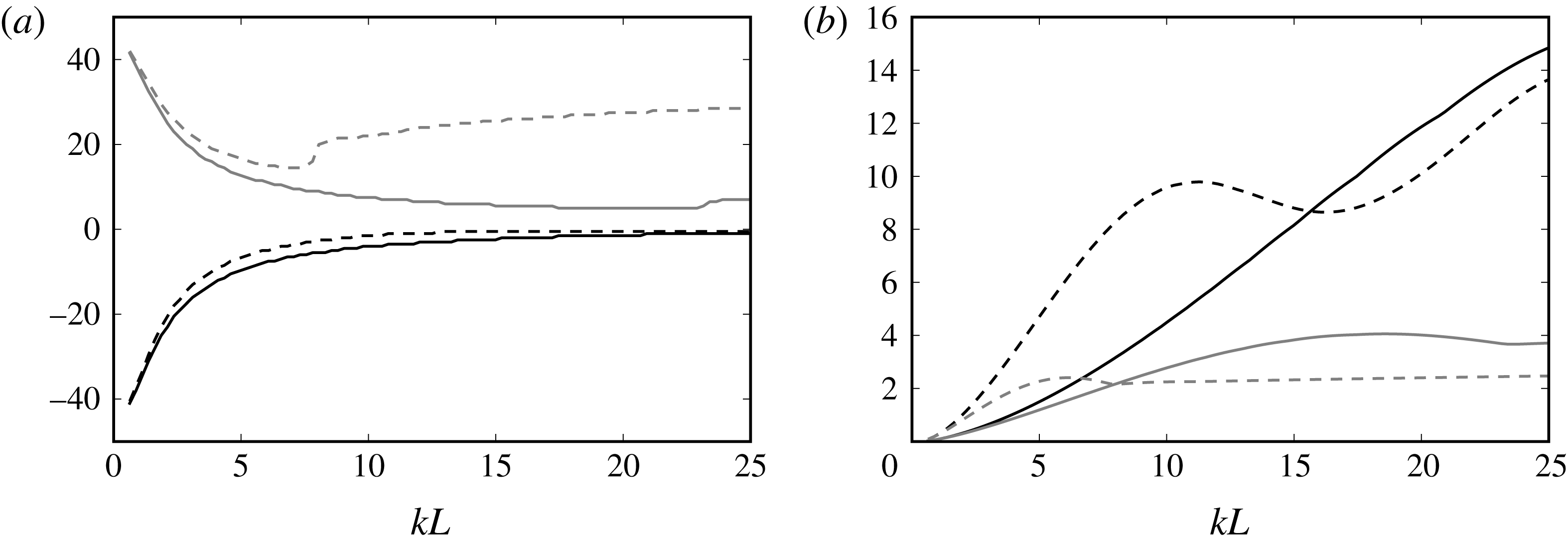
The evolutions of the directions and magnitudes of the maxima of the scattered directivity are plotted in figure 5. For the weaker vortex with
 $M_{v}=0.05$
, it confirms that the maxima of the directivity move closer to
 $\unicode[STIX]{x1D703}=0^{\circ }$
when the Helmholtz number
 $kL$
increases. The main beam is found in the lower half (
 $\unicode[STIX]{x1D703}<0$
) and its amplitude grows with
 $kL$
. In contrast, the beam in the upper half is weaker and its amplitude does not seem to evolve much at high frequency.
For the stronger vortex, we see that the main beam (found for
 $\unicode[STIX]{x1D703}<0$
) moves more rapidly towards
 $\unicode[STIX]{x1D703}=0$
. However, the beam in the upper half (
 $\unicode[STIX]{x1D703}>0$
) moves towards the axis before moving away when
 $kL>7$
. The amplitude of the main beam increases more rapidly for Helmholtz numbers up to
 $kL=10$
compared with the case
 $M_{v}=0.05$
. It then stops growing for
 $10<kL<16$
before growing again at higher Helmholtz numbers. The amplitude of the main beam in the upper half is lower than that of the case
 $M_{v}=0.05$
and is almost constant for
 $kL>8$
.
The evolution of (a) the angular positions
 $\unicode[STIX]{x1D703}$
and (b) the amplitudes
 $|D(\unicode[STIX]{x1D703})|$
of the maxima of the scattered directivity with the incident wave Helmholtz number for
 $\unicode[STIX]{x1D703}>0^{\circ }$
(grey) and
 $\unicode[STIX]{x1D703}<0^{\circ }$
(black) with a vortex magnitude of
 $M_{v}=0.05$
(solid lines) and
 $M_{v}=0.15$
(dashed lines).

2.4.2 Conservation of acoustic energy
Since the incident sound wave interacts with a non-uniform base flow with non-zero mean vorticity, there is no guarantee that the acoustic energy is conserved by the scattering. However, Lighthill (Reference Lighthill1953) showed, in the small-wavelength limit, that there is conservation of the acoustic energy, and Howe’s model (Howe Reference Howe1973) indicates that the acoustic energy is conserved for frozen turbulence. The scattering process is therefore assumed to redistribute the acoustic energy spatially but not to act as a source or sink of energy. The validity of this assumption can be assessed using the solution from the semianalytical model developed in § 2.2.
The acoustic power is calculated over a circle surrounding the vortex with a radius
 $r$
sufficiently large to be located where the mean flow is negligible,
 $$\begin{eqnarray}W_{t}=\int _{0}^{2\unicode[STIX]{x03C0}}\frac{1}{2}\text{Re}(p^{\prime \ast }u_{r}^{\prime })r\,\text{d}\unicode[STIX]{x1D703},\end{eqnarray}$$
where
 $u_{r}^{\prime }$
is the radial acoustic velocity and
 $^{\ast }$
is the complex conjugate. It is possible to show that the total power is the sum of two terms,
 $W_{t}=W_{s}+W_{si}$
, where
 $W_{s}$
is the power associated with the scattered field in isolation and
 $W_{si}$
is the additional term due to the interference between the incident plane wave and the scattered field (the details of the derivation can be found in appendix A),
 $$\begin{eqnarray}W_{s}=\frac{2}{\unicode[STIX]{x1D70C}_{\infty }c_{\infty }k}\mathop{\sum }_{m=-\infty }^{+\infty }|A_{m}|^{2},\quad W_{si}=\frac{2}{\unicode[STIX]{x1D70C}_{\infty }c_{\infty }k}\mathop{\sum }_{m=-\infty }^{+\infty }\text{Re}(\text{i}^{m}A_{m}P^{\ast }).\end{eqnarray}$$
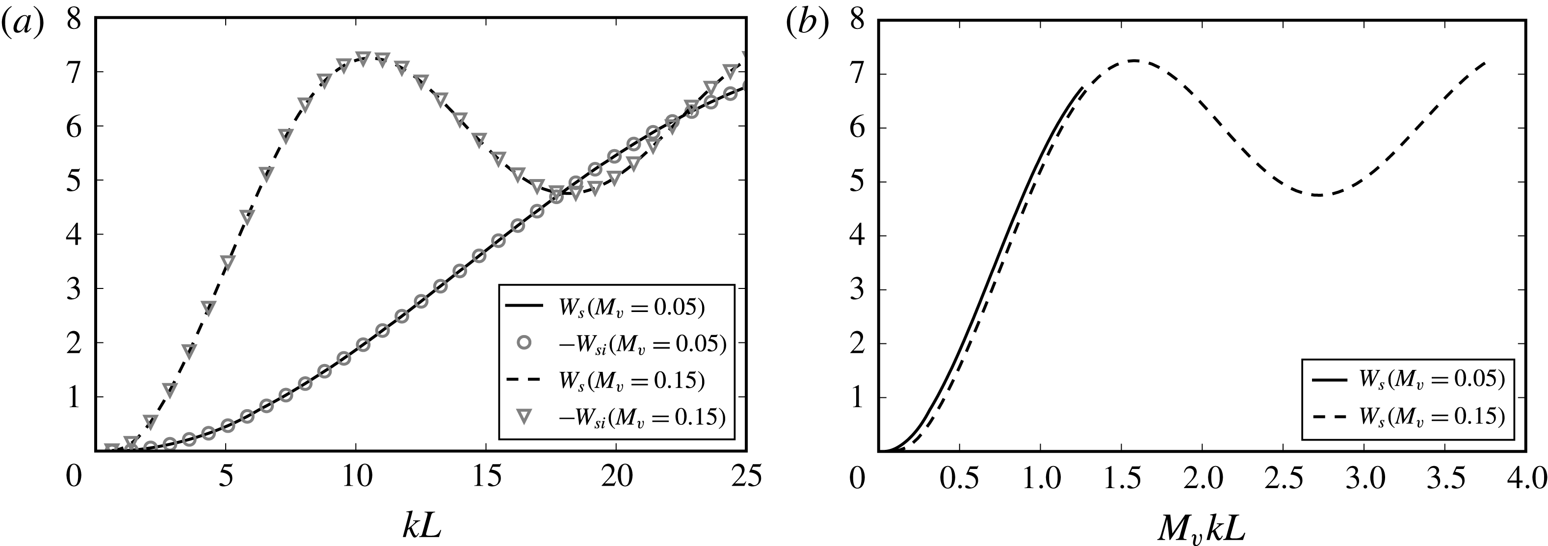
These quantities are plotted in figure 6(a) over a range of Helmholtz numbers
 $kL$
and for two vortex Mach numbers
 $M_{v}=0.05$
and 0.15. It is clear that we have
 $W_{s}=-W_{si}$
, which implies that the total power is zero and that the acoustic energy is indeed conserved. The scattering by the vortex therefore appears not to transfer acoustic energy to vortical disturbances. It is clear that the scattered power increases much more rapidly with frequency in the case
 $M_{v}=0.15$
compared with
 $M_{v}=0.05$
, at least for
 $kL<10$
. For
 $kL>10$
,
 $W_{s}$
oscillates for
 $M_{v}=0.15$
but continues to increase for
 $M_{v}=0.05$
, until
 $W_{s}$
is similar for the two vortex Mach numbers. Finally, it is interesting to note from figure 6(b) that there is a good collapse of the results when plotted as functions of
 $M_{v}kL$
, at least for low frequencies.
The acoustic power of the scattered field in isolation (
 $W_{s}$
) and of the interference between the scattered and incident fields (
 $W_{si}$
) for
 $M_{v}=0.05$
and 0.15, plotted against (a)
 $kL$
and (b)
 $M_{v}kL$
.

3 Scattering of a harmonic plane wave by a convected vortex
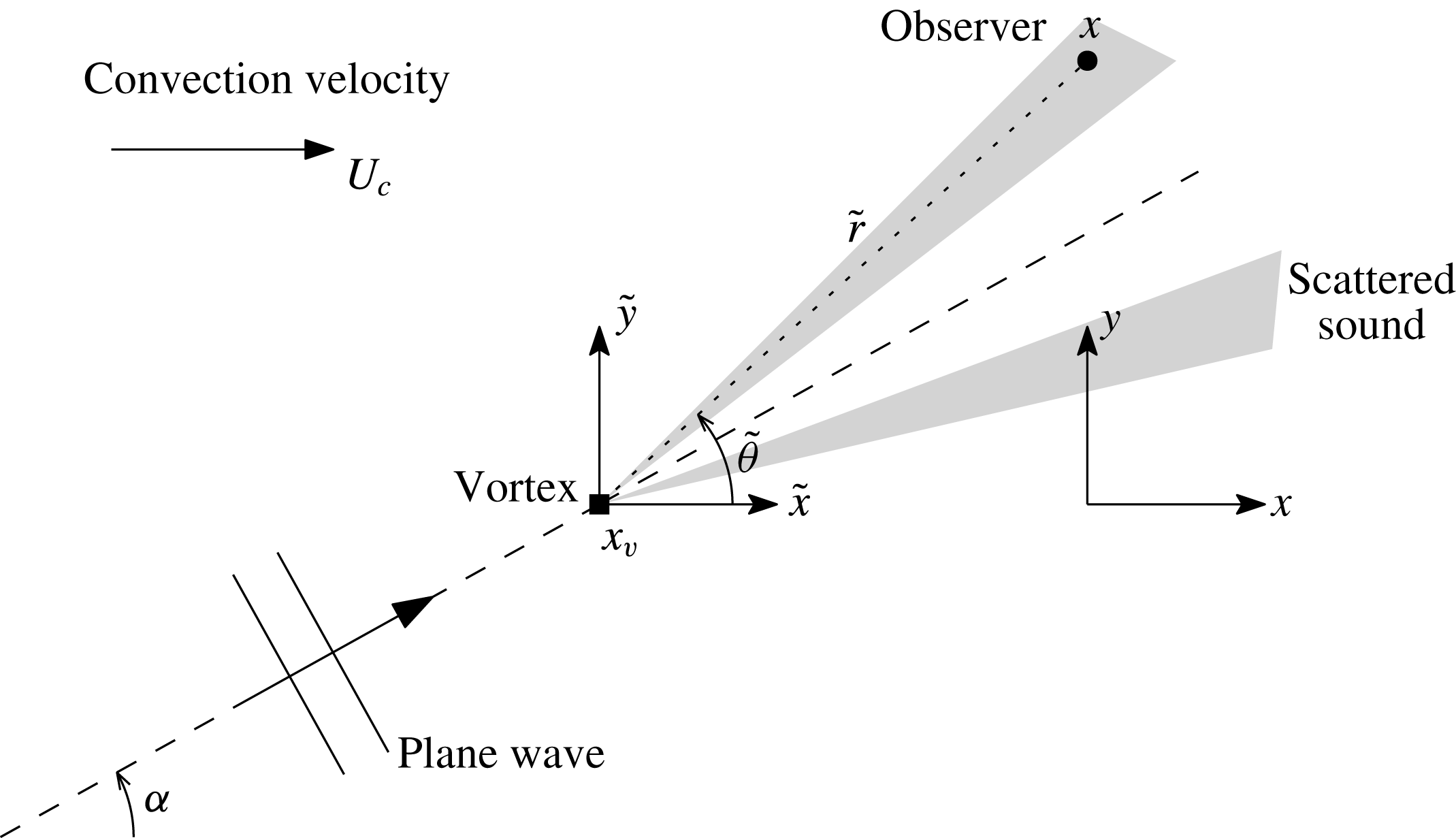
We now consider the case of a single vortex convected by a uniform background flow, as depicted in figure 7. The uniform flow is along the
 $x$
axis and has velocity
 $U_{c}$
and Mach number
 $M_{c}=U_{c}/c_{\infty }$
. The position of the vortex is given by
 $x_{v}=U_{c}t$
and
 $y_{v}=0$
. The incident sound field is a plane wave with direction
 $\unicode[STIX]{x1D6FC}$
(measured from the positive
 $x$
axis) and angular frequency
 $\unicode[STIX]{x1D714}_{s}$
. We are interested in the pressure signal measured by a fixed observer located at
 $(x,y)$
.
In addition to the spatial scattering of sound discussed in the previous section, the motion of the vortex relative to the observer leads to spectral broadening of the initial sound spectrum (a pure tone in this case). This combined effect of the Doppler shift together with the vortex scattering is described using the frequency-domain semianalytical model and the time-domain numerical model.
Schematic of the scattering of an acoustic plane wave by a convected vortex.

3.1 Semianalytical model
In the case of an incident plane wave, the semianalytical model presented in § 2.2 can be generalised to include the vortex convection. This is achieved by changing from the fixed frame of reference
 $(x,y)$
used above to a frame of reference
 $(\tilde{x},{\tilde{y}})$
moving with the vortex. These two coordinate systems are related by
 $$\begin{eqnarray}\tilde{x}=x-x_{v}=x-U_{c}t,\quad {\tilde{y}}=y-y_{v}=y.\end{eqnarray}$$
When using the moving frame of reference
 $(\tilde{x},{\tilde{y}})$
, we recover a situation with no mean flow at infinity and a steady base flow; thus, the model from § 2.2 can be used. There are, however, two important changes associated with this change of frame of reference.
First, in the fixed frame of reference, the pressure field of the incident plane wave is
 $$\begin{eqnarray}p(x,y,t)=\exp (\text{i}\unicode[STIX]{x1D714}_{s}t-\text{i}kx\cos \unicode[STIX]{x1D6FC}-\text{i}ky\sin \unicode[STIX]{x1D6FC}),\end{eqnarray}$$
where the wavenumber
 $k=\unicode[STIX]{x1D714}_{s}/(c_{\infty }+U_{c}\cos \unicode[STIX]{x1D6FC})$
accounts for the fact that the wave is propagating in a uniform mean flow. This definition of
 $k$
is a direct consequence of the dispersion relation for acoustic plane waves in a uniform flow,
 $$\begin{eqnarray}k^{2}=\left(\frac{\unicode[STIX]{x1D714}_{s}}{c_{\infty }+U_{c}\cos \unicode[STIX]{x1D6FC}}\right)^{2};\end{eqnarray}$$
see Morse & Ingard (Reference Morse and Ingard1968, § 11.1) or Goldstein (Reference Goldstein1976, § 1.3.2) for more details. In the frame of reference moving with the vortex, the incident field remains a plane wave with a wavenumber
 $k$
,
 $$\begin{eqnarray}p(\tilde{x},{\tilde{y}},t)=\exp (\text{i}\unicode[STIX]{x1D714}_{v}t-\text{i}k\tilde{x}\cos \unicode[STIX]{x1D6FC}-\text{i}k{\tilde{y}}\sin \unicode[STIX]{x1D6FC}).\end{eqnarray}$$
Since the propagation velocity of the acoustic waves relative to the vortex is
 $c_{\infty }$
, the incident plane wave is perceived in the moving frame at a Doppler-shifted frequency
 $\unicode[STIX]{x1D714}_{v}$
given by
 $$\begin{eqnarray}\unicode[STIX]{x1D714}_{v}=kc_{\infty }=\frac{\unicode[STIX]{x1D714}_{s}}{1+M_{c}\cos \unicode[STIX]{x1D6FC}}.\end{eqnarray}$$
For any observer moving with the vortex, the incident and scattered sound fields are both time-harmonic with frequency
 $\unicode[STIX]{x1D714}_{v}$
. It is only in the special case of a plane wave that the incident field remains tonal after changing the frame of reference. A more complex sound field, such as that radiated by a time-harmonic point source, will not be perceived as tonal noise in the moving frame of reference. This will be considered in § 4.
Second, the scattered pressure signal measured by a fixed observer located at
 $(x,y)$
in the fixed frame of reference can be obtained using (2.9),
 $$\begin{eqnarray}p_{s}^{\prime }(t)=\mathop{\sum }_{m=-\infty }^{+\infty }A_{m}\mathit{H}_{m}^{(2)}[k\tilde{r}(t)]\exp \{\text{i}\unicode[STIX]{x1D714}_{v}t-\text{i}m[\tilde{\unicode[STIX]{x1D703}}(t)-\unicode[STIX]{x1D6FC}]\},\end{eqnarray}$$
where
 $(\tilde{r},\tilde{\unicode[STIX]{x1D703}})$
are the polar coordinates centred on the vortex,
 $$\begin{eqnarray}\tilde{r}(t)=\sqrt{\tilde{x}(t)^{2}+{\tilde{y}}(t)^{2}},\quad \tilde{\unicode[STIX]{x1D703}}(t)=\tan ^{-1}[{\tilde{y}}(t)/\tilde{x}(t)].\end{eqnarray}$$
It should be noted that in (3.6) the coefficients
 $A_{m}$
are calculated at the frequency
 $\unicode[STIX]{x1D714}_{v}$
and that the angular orientation of the scattered field is shifted by the angle of incidence
 $\unicode[STIX]{x1D6FC}$
of the plane wave. If the observer remains in the acoustic far field from the vortex, we can use the asymptotic expression (2.10) to write
 $$\begin{eqnarray}p_{s}^{\prime }(t)\simeq \frac{D[\tilde{\unicode[STIX]{x1D703}}(t)-\unicode[STIX]{x1D6FC}]}{\sqrt{\tilde{r}(t)}}\exp \{\text{i}\unicode[STIX]{x1D714}_{v}[t-\tilde{r}(t)/c_{\infty }]\}.\end{eqnarray}$$
In addition to the Doppler shift (3.5) there is also a Doppler shift associated with the relative motion between the observer and the vortex. In (3.8), this is captured by the time dependence of
 $\tilde{r}$
in the argument of the exponential. We can define the instantaneous angular frequency
 $\unicode[STIX]{x1D714}_{o}$
perceived by the observer as follows:
 $$\begin{eqnarray}\unicode[STIX]{x1D714}_{o}(t)=\frac{\unicode[STIX]{x2202}}{\unicode[STIX]{x2202}t}\{\unicode[STIX]{x1D714}_{v}[t-\tilde{r}(t)/c_{\infty }]\}=\unicode[STIX]{x1D714}_{v}[1+M_{c}\cos \tilde{\unicode[STIX]{x1D703}}(t)]=\unicode[STIX]{x1D714}_{s}\frac{1+M_{c}\cos \tilde{\unicode[STIX]{x1D703}}(t)}{1+M_{c}\cos \unicode[STIX]{x1D6FC}}.\end{eqnarray}$$
It should be noted that this second Doppler shift can also be understood in the frame of reference moving with the vortex. In this frame of reference, the vortex is emitting scattered waves in a quiescent medium with wavenumber
 $k$
. As the observer is in motion, it is receiving waves with a relative propagation velocity
 $c_{\infty }+U_{c}\cos \tilde{\unicode[STIX]{x1D703}}(t)$
at a frequency
 $$\begin{eqnarray}\unicode[STIX]{x1D714}_{o}(t)=k(c_{\infty }+U_{c}\cos \tilde{\unicode[STIX]{x1D703}}(t))=\unicode[STIX]{x1D714}_{s}\frac{1+M_{c}\cos \tilde{\unicode[STIX]{x1D703}}(t)}{1+M_{c}\cos \unicode[STIX]{x1D6FC}}.\end{eqnarray}$$
The ratio between the two Doppler factors shows that the effective frequency perceived by the observer is the result of two Doppler shifts, the first due to the relative motion between the source and the vortex, the second due to the relative motion between the vortex and the observer.
3.2 Numerical model
The numerical method presented in § 2.1 can also be used with an unsteady base flow as the governing equations (2.1) remain valid when the base flow properties
 $\boldsymbol{u}$
,
 $\unicode[STIX]{x1D70C}$
and
 $p$
are varying in time. It is useful to separate the base flow into steady and unsteady components by writing
 $(\unicode[STIX]{x1D70C},\boldsymbol{u},p)=(\unicode[STIX]{x1D70C}_{0},\boldsymbol{u}_{0},p_{0})+(\unicode[STIX]{x1D70C}_{t},\boldsymbol{u}_{t},p_{t})$
, where the subscripts
 $0$
and
 $t$
denote the steady and unsteady components respectively. For the convected vortex, these are given by
 $$\begin{eqnarray}\boldsymbol{u}_{0}=U_{c}\boldsymbol{e}_{x},\quad p_{0}=p_{\infty },\quad \unicode[STIX]{x1D70C}_{0}=\unicode[STIX]{x1D70C}_{\infty }\end{eqnarray}$$
and
 $$\begin{eqnarray}\left.\begin{array}{@{}c@{}}\boldsymbol{u}_{t}(\tilde{r})=U_{v}{\displaystyle \frac{r}{L}}\exp \left[{\displaystyle \frac{1}{2}}(1-\tilde{r}^{2}/L^{2})\right]\boldsymbol{e}_{\unicode[STIX]{x1D703}},\\ p_{t}(\tilde{r})=p_{\infty }\left[1-{\displaystyle \frac{\unicode[STIX]{x1D6FE}-1}{2}}M_{v}^{2}\exp (1-\tilde{r}^{2}/L^{2})\right]^{\unicode[STIX]{x1D6FE}/(\unicode[STIX]{x1D6FE}-1)}-p_{\infty },\\ \unicode[STIX]{x1D70C}_{t}(\tilde{r})=\unicode[STIX]{x1D70C}_{\infty }[1+p_{t}(\tilde{r})/p_{\infty }]^{1/\unicode[STIX]{x1D6FE}}-\unicode[STIX]{x1D70C}_{\infty },\end{array}\right\}\end{eqnarray}$$
where the unit vectors in Cartesian coordinates are denoted by
 $(\boldsymbol{e}_{x},\boldsymbol{e}_{y})$
.
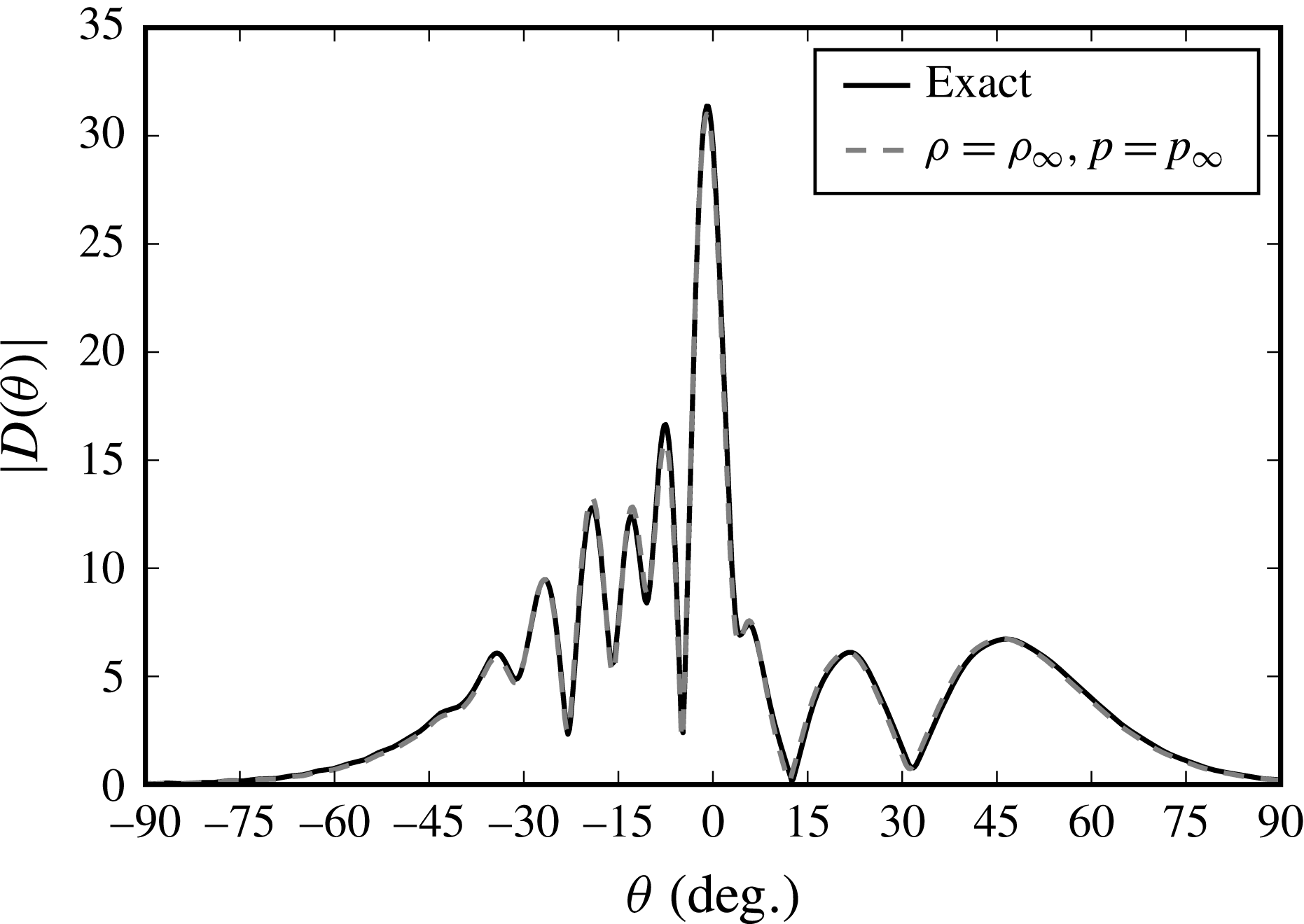
In the present work, it is assumed that the unsteady density and pressure components associated with the vortex in the base flow do not have a significant influence on the scattering of the acoustic wave. Appendix B shows that
 $p_{t}$
and
 $\unicode[STIX]{x1D70C}_{t}$
can indeed be ignored without any significant change in the solutions.
After splitting the base flow as explained above, noting that
 $\unicode[STIX]{x1D735}\boldsymbol{\cdot }\boldsymbol{u}_{t}=0$
from the definition of
 $\boldsymbol{u}_{t}$
in (3.12) and ignoring the terms in
 $p_{t}$
and
 $\unicode[STIX]{x1D70C}_{t}$
, the governing equations (2.1) can be written as
 $$\begin{eqnarray}\left.\begin{array}{@{}c@{}}{\displaystyle \frac{\unicode[STIX]{x2202}\unicode[STIX]{x1D70C}^{\prime }}{\unicode[STIX]{x2202}t}}+\boldsymbol{u}_{0}\boldsymbol{\cdot }\unicode[STIX]{x1D735}\unicode[STIX]{x1D70C}^{\prime }+\boldsymbol{u}^{\prime }\boldsymbol{\cdot }\unicode[STIX]{x1D735}\unicode[STIX]{x1D70C}_{0}+\unicode[STIX]{x1D70C}_{0}\unicode[STIX]{x1D735}\boldsymbol{\cdot }\boldsymbol{u}^{\prime }+\unicode[STIX]{x1D70C}^{\prime }\unicode[STIX]{x1D735}\boldsymbol{\cdot }\boldsymbol{u}_{0}=-\boldsymbol{u}_{t}\boldsymbol{\cdot }\unicode[STIX]{x1D735}\unicode[STIX]{x1D70C}^{\prime },\\ {\displaystyle \frac{\unicode[STIX]{x2202}\boldsymbol{u}^{\prime }}{\unicode[STIX]{x2202}t}}+(\boldsymbol{u}_{0}\boldsymbol{\cdot }\unicode[STIX]{x1D735})\boldsymbol{u}^{\prime }+(\boldsymbol{u}^{\prime }\boldsymbol{\cdot }\unicode[STIX]{x1D735})\boldsymbol{u}_{0}+{\displaystyle \frac{\unicode[STIX]{x1D735}p^{\prime }}{\unicode[STIX]{x1D70C}_{0}}}-\unicode[STIX]{x1D70C}^{\prime }{\displaystyle \frac{\unicode[STIX]{x1D735}p_{0}}{\unicode[STIX]{x1D70C}_{0}^{2}}}=-(\boldsymbol{u}_{t}\boldsymbol{\cdot }\unicode[STIX]{x1D735})\boldsymbol{u}^{\prime }-(\boldsymbol{u}^{\prime }\boldsymbol{\cdot }\unicode[STIX]{x1D735})\boldsymbol{u}_{t},\\ {\displaystyle \frac{\unicode[STIX]{x2202}p^{\prime }}{\unicode[STIX]{x2202}t}}+\boldsymbol{u}_{0}\boldsymbol{\cdot }\unicode[STIX]{x1D735}p^{\prime }+\boldsymbol{u}^{\prime }\boldsymbol{\cdot }\unicode[STIX]{x1D735}p_{0}+\unicode[STIX]{x1D6FE}p_{0}\unicode[STIX]{x1D735}\boldsymbol{\cdot }\boldsymbol{u}^{\prime }+\unicode[STIX]{x1D6FE}p^{\prime }\unicode[STIX]{x1D735}\boldsymbol{\cdot }\boldsymbol{u}_{0}=-\boldsymbol{u}_{t}\boldsymbol{\cdot }\unicode[STIX]{x1D735}p^{\prime },\end{array}\right\}\end{eqnarray}$$
where the terms with
 $\boldsymbol{u}_{t}$
have been gathered on the right-hand side. The wave operator on the left-hand side only involves the steady component of the base flow, while the right-hand side is responsible for the unsteady scattering of sound. These equations are solved using the time-domain finite-difference method described in § 2.1.
The rectangular computational domain is defined by
 $-42.5L<x<42.5L$
and
 $-12L<y<18L$
and uses a constant grid resolution of
 $\unicode[STIX]{x0394}x=\unicode[STIX]{x0394}y=L/10$
for computations with acoustic wavelengths
 $\unicode[STIX]{x1D706}>L$
. For computations with smaller acoustic wavelengths, the grid resolution ensures 12 points per wavelength and the domain size in the
 $y$
direction is reduced to
 $-8L<y<15L$
. The incoming sound field (plane wave or monopole) is introduced to the domain through a 20-point wide sponge layer adjacent to the lower boundary. An additional dissipative sponge layer with 50 grid points is added along the upper boundary. The simulation is first performed without the vortex until the incident sound field is well established throughout the computational domain. The unsteady base flow
 $\boldsymbol{u}_{t}$
including the vortex is then considered, with the initial position of the vortex chosen upstream of the computational domain so that it enters the domain smoothly. The pressure signals at a number of observer positions are then recorded during the traversal of the vortex.
3.3 Discussion of results
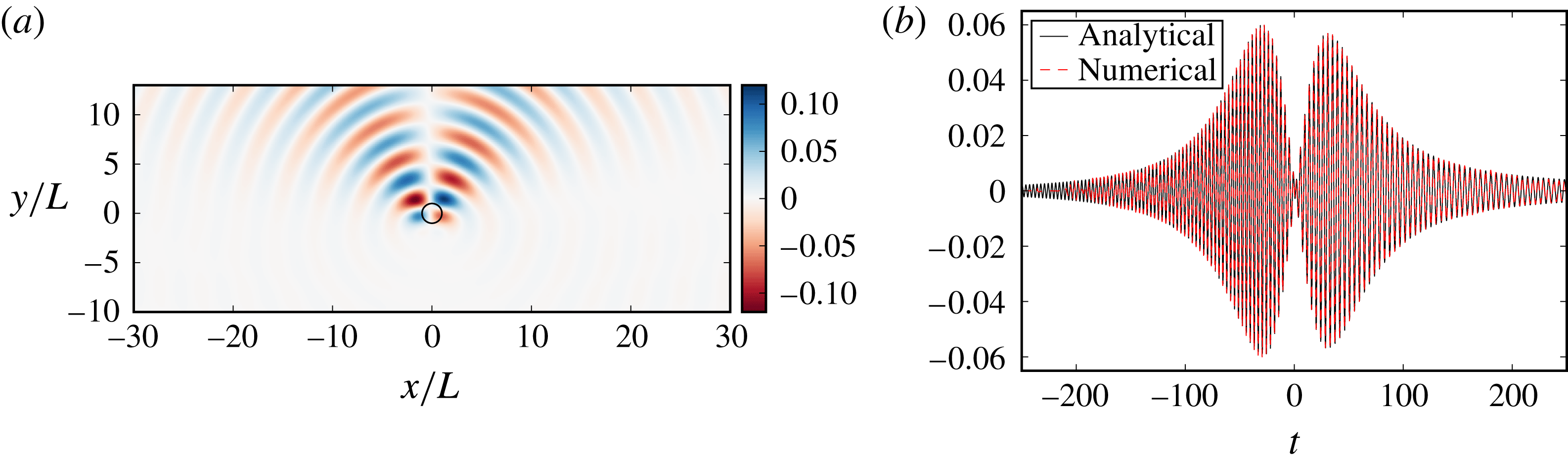
Figure 8 shows examples of results for the scattering of a plane wave by a convected vortex. The time evolution of the pressure field during the passage of the vortex is presented in movie 1 as supplementary material available online at https://doi.org/10.1017/jfm.2018.94. The scattered field is very similar to that observed for a stationary vortex in § 2.3 as it is composed of two beams radiating on either side of the direction
 $\unicode[STIX]{x1D6FC}$
. Due to the convection of the vortex, this scattered field is also moving in the
 $x$
direction. Figure 8(b) shows the scattered pressure recorded at a fixed position
 $x=0$
,
 $y=10L$
so that the vortex passes just below the observer at
 $t=0$
. This signal is formed of two wavepackets associated with the two scattered beams. Apart from the initial transient in the time-domain simulation, there is excellent agreement between the two methods. The semianalytical model will therefore be used for the remainder of this section.
The scattered pressure
 $p_{s}^{\prime }$
for a plane wave with direction
 $\unicode[STIX]{x1D6FC}=\unicode[STIX]{x03C0}/2$
scattered by a vortex of strength
 $M_{v}=0.05$
convected at a velocity
 $M_{c}=0.176$
. The frequency is
 $kL=\unicode[STIX]{x03C0}/2$
. (a) Snapshot of the scattered field in the time-domain numerical simulation at
 $t=0$
(the circle shows the position of the vortex). (b) Pressure signal at
 $x=0$
,
 $y=10L$
.

The scattered pressure given by (3.6) at
 $x=0$
,
 $y=10L$
for different plane wave directions
 $\unicode[STIX]{x1D6FC}$
. The parameters are
 $M_{v}=0.05$
,
 $M_{c}=0.176$
and
 $k_{0}L=\unicode[STIX]{x03C0}/2$
. (a) Pressure amplitude
 $|p_{s}^{\prime }|$
. (b) Instantaneous frequency
 $\unicode[STIX]{x1D714}_{o}(t)$
given by (3.9) normalised by the source frequency
 $\unicode[STIX]{x1D714}_{s}$
.

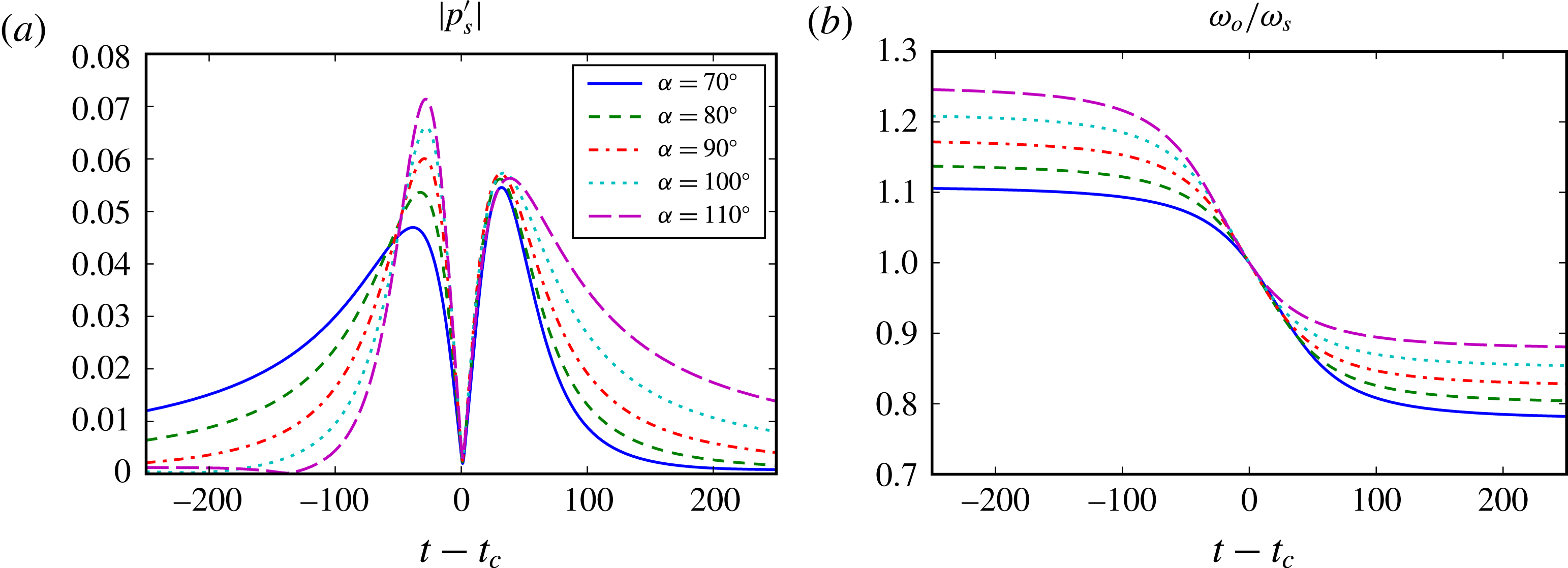
Figure 9 shows the amplitude and instantaneous frequency of the scattered pressure recorded at
 $x=0$
,
 $y=10L$
for different plane wave directions. It should be noted that these results are plotted as functions of
 $t-t_{c}$
, where
 $t_{c}=y_{m}/(U_{c}\tan \unicode[STIX]{x1D6FC})$
is when the direction between
 $\boldsymbol{x}_{v}$
and
 $\boldsymbol{x}$
coincides with the plane wave direction, i.e. when
 $\tilde{\unicode[STIX]{x1D703}}(t)=\unicode[STIX]{x1D6FC}$
. This corresponds to the time when the observer is located between the two scattered beams and the scattered pressure amplitude is close to zero.
From (3.8), we can see that
 $|p_{s}^{\prime }|$
is the combination of the directivity
 $D(\tilde{\unicode[STIX]{x1D703}}-\unicode[STIX]{x1D6FC})$
of the vortex scattering and the cylindrical spreading
 $1/\sqrt{\tilde{r}}$
. The amplitude of the scattered field changes significantly as
 $\unicode[STIX]{x1D6FC}$
is varied, especially the amplitude of the first wavepacket. This can be explained by noting that for
 $\unicode[STIX]{x1D6FC}<90^{\circ }$
the first beam is closer to the
 $x$
axis and will therefore be received by the observer when the vortex is further away from the microphone. Also important is the change in amplitude for large values of
 $|t|$
, i.e. when the vortex is far from the observer.
Figure 9(b) shows the evolution of the instantaneous frequency
 $\unicode[STIX]{x1D714}_{o}$
defined by (3.9) as the vortex is convected past the observer. As expected, the frequency of the signal received by the observer is originally higher than the source frequency
 $\unicode[STIX]{x1D714}_{s}$
(for
 $t<t_{c}$
) but then becomes smaller (for
 $t>t_{c}$
). The transition occurs when
 $\unicode[STIX]{x1D714}_{o}=\unicode[STIX]{x1D714}_{s}$
, and, as seen from (3.9), this corresponds indeed to
 $t=t_{c}$
and
 $\tilde{\unicode[STIX]{x1D703}}=\unicode[STIX]{x1D6FC}$
. This implies that the first wavepacket always contains higher frequencies (
 $\unicode[STIX]{x1D714}>\unicode[STIX]{x1D714}_{s}$
) and the second wavepacket lower frequencies (
 $\unicode[STIX]{x1D714}<\unicode[STIX]{x1D714}_{s}$
). A subtle point to note is that whether the observer perceives frequencies above or below
 $\unicode[STIX]{x1D714}_{s}$
is not solely explained by the vortex relative motion towards, or away from, the observer. Figure 7 corresponds to a situation where the vortex is moving towards the observer but the second beam, which is pointing towards the observer at that particular instant, will be perceived at frequencies below
 $\unicode[STIX]{x1D714}_{s}$
. This is because the effective frequency
 $\unicode[STIX]{x1D714}_{o}$
also includes the Doppler shift
 $1/(1+M_{c}\cos \unicode[STIX]{x1D6FC})$
.
Even though the incident sound field is tonal, the signal recorded by the observer contains a range of frequencies. This is described in (3.9) by the Doppler shift
 $1+M_{c}\cos \tilde{\unicode[STIX]{x1D703}}(t)$
, which accounts for the motion of the vortex relative to the observer. It should be noted that the Doppler shift
 $1+M_{c}\cos \unicode[STIX]{x1D6FC}$
expressing the frequency received by the vortex does not represent spectral broadening since the incident wave remains time-harmonic in the frame of reference moving with the vortex. This shift remains constant during the passage of the vortex. Its effect is visible in figure 9(b), where
 $\unicode[STIX]{x1D714}_{o}$
increases or decreases when the direction of the plane wave is varied.
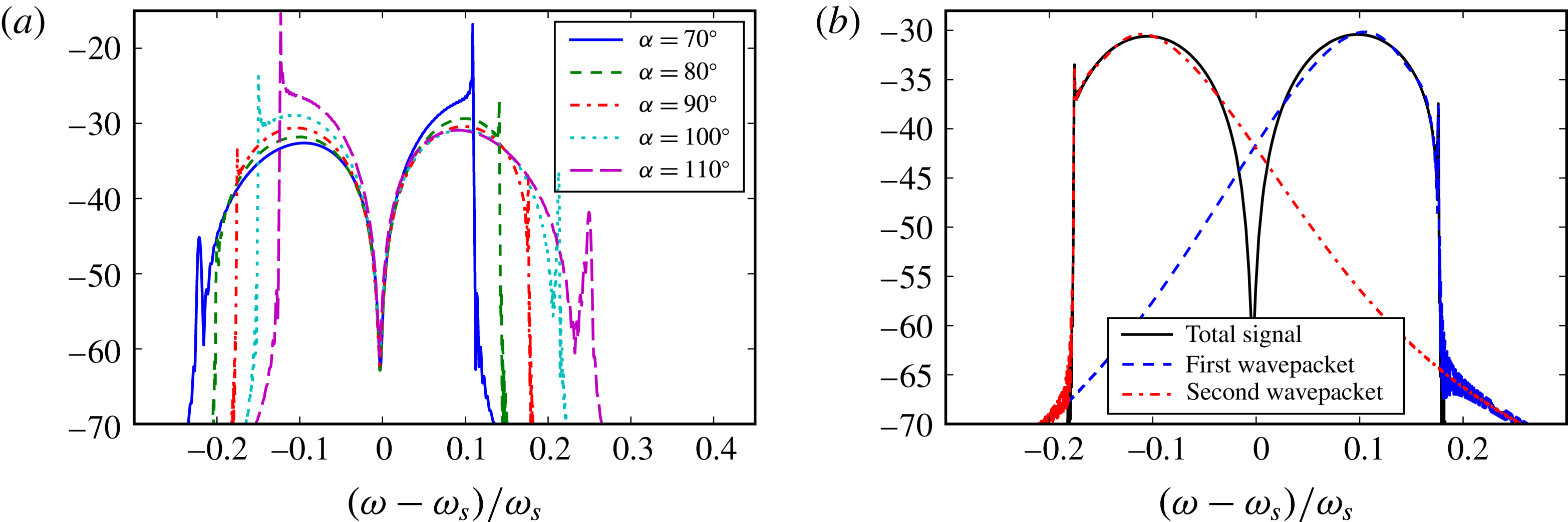
Figure 9(b) shows the range of frequencies received by the observer, and this is also seen in the spectrum of the signals, shown in figure 10(a), where decibels (dB) are defined as
 $10\log _{10}(p^{\prime 2}/p_{ref}^{2})$
, with a reference
 $p_{ref}=1$
. It is clear from (3.9), and in figure 9(b) as well, that the perceived frequency
 $\unicode[STIX]{x1D714}_{o}$
varies between
 $\unicode[STIX]{x1D714}_{s}(1-M_{c})/(1+M_{c}\cos \unicode[STIX]{x1D6FC})$
and
 $\unicode[STIX]{x1D714}_{s}(1+M_{c})/(1+M_{c}\cos \unicode[STIX]{x1D6FC})$
. This is also visible in the spectra in figure 10(a), which drop sharply outside this frequency range. These spectra all show a typical pattern with two sidelobes located on either side of the source frequency, although the amplitudes and widths of these sidelobes vary with the direction
 $\unicode[STIX]{x1D6FC}$
of the plane wave.
The peaks in the spectra are only present when considering a plane wave in two dimensions. As
 $|t|\rightarrow \infty$
, the instantaneous frequency
 $\unicode[STIX]{x1D714}_{o}$
tends to
 $\unicode[STIX]{x1D714}_{s}(1\pm M_{c})/(1+M_{c}\cos \unicode[STIX]{x1D6FC})$
and
 $|p_{s}^{\prime }|$
decreases like
 $1/\sqrt{r}\sim 1/|t|^{1/2}$
. This rate of decay is not sufficient to ensure that the Fourier transform of
 $p_{s}^{\prime }$
is finite, and singularities are expected at these two frequencies in the spectra (Davies Reference Davies2012). In the case of the point source considered in § 4, the signals will decay like
 $1/r\sim 1/|t|$
when
 $|t|\rightarrow \infty$
(due to the cylindrical spreading of the waves from the source to the vortex and from the vortex to the observer) and the Fourier transforms are regular.
It is possible to further understand the presence of these sidelobes in the spectrum of the scattered field. The pressure signal for
 $\unicode[STIX]{x1D6FC}=90^{\circ }$
is shown in figure 8. It is composed of two wavepackets (for
 $t<0$
and
 $t>0$
), and the spectra corresponding to each wavepacket taken individually are shown in figure 10(b). This confirms that the first wavepacket is responsible for the high-frequency sidelobe (
 $\unicode[STIX]{x1D714}>\unicode[STIX]{x1D714}_{s}$
) whereas the second wavepacket contains the low-frequency sidelobe (
 $\unicode[STIX]{x1D714}<\unicode[STIX]{x1D714}_{s}$
).
Sound pressure levels (in dB
 $/$
Hz ref. 1) at
 $x=0$
,
 $y=10L$
. The parameters are
 $M_{v}=0.05$
,
 $M_{c}=0.176$
and
 $kL=\unicode[STIX]{x03C0}/2$
. (a) Comparison for different plane wave directions
 $\unicode[STIX]{x1D6FC}$
. (b) Individual spectra of the two wavepackets for
 $\unicode[STIX]{x1D6FC}=90^{\circ }$
.

To summarise, although the incident sound field is tonal in both the fixed and moving reference frames (because it is a plane wave), the scattered field is only tonal in the reference frame moving with the vortex. When observed in the fixed reference frame, the scattered field contains a range of frequencies. It is the Doppler shift originating from the motion of the vortex relative to the observer that is responsible for the spectral broadening of the sound field. In addition, the spectrum of the scattered field for a fixed observer is a direct consequence of the directivity of the scattering by a steady vortex. The presence of a sidelobe on each side of the source frequency can be directly attributed to the fact that the scattered field is formed of two beams at the frequency considered, with each beam generating one sidelobe.
4 Scattering of more complex sound fields by a convected vortex
When the incident sound field is a time-harmonic plane wave, it is still perceived as tonal noise by the vortex (although at a Doppler-shifted frequency
 $\unicode[STIX]{x1D714}_{v}$
). This is not the case when considering a more complex sound field, such as that generated by a point mass source fixed relative to the observer, which is the configuration considered in this section. While this sound field is tonal in the fixed frame of reference, it is perceived in the moving frame of reference as containing a range of frequencies. The frequency-domain model presented in §§ 2.2 and 3.1 is therefore not well adapted to this situation, and it is preferable to use the time-domain numerical model instead.
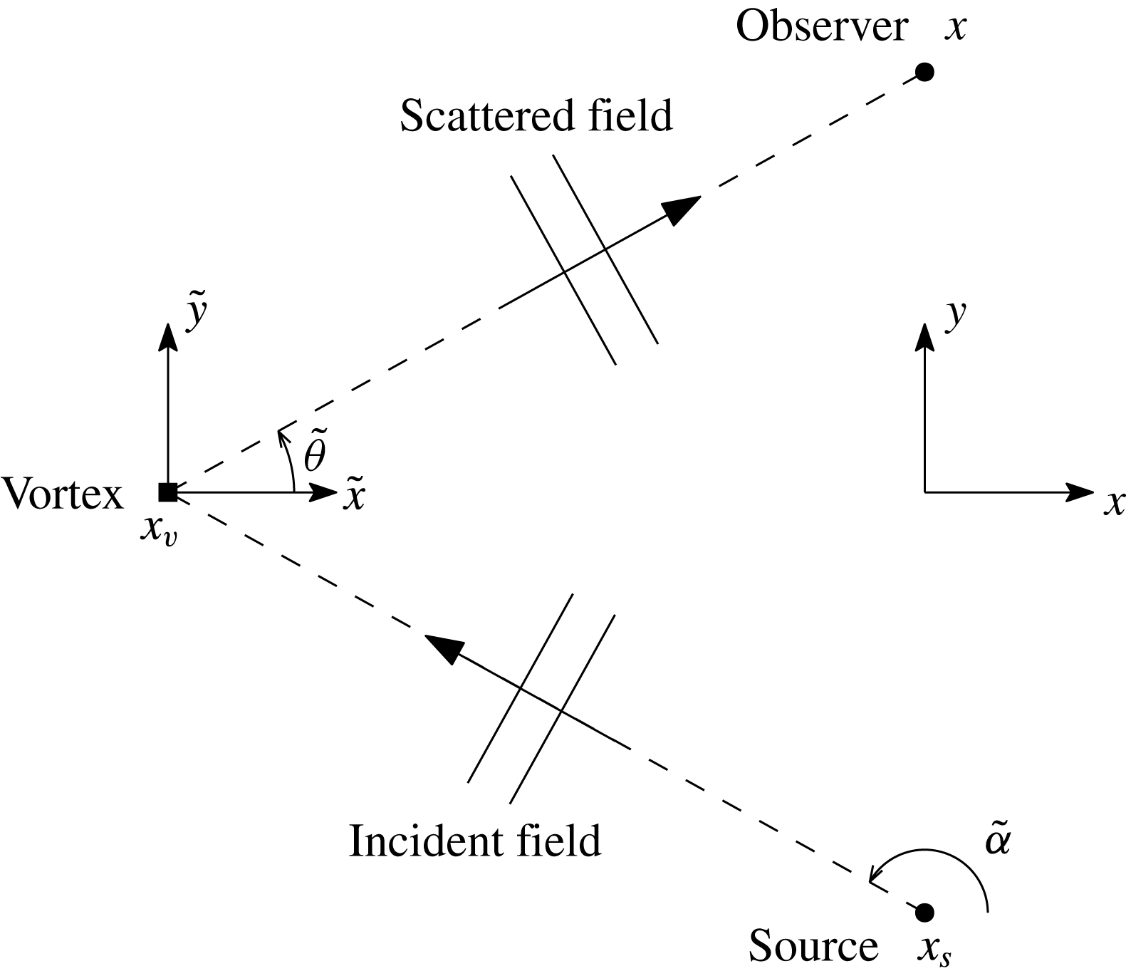
Schematic of the scattering of the sound emitted by a fixed point source by a convected vortex.

4.1 Doppler shifts
Before we use the numerical model, it is still useful to derive a simple expression for the Doppler shifts involved in the change in frequency between the point source, the vortex and the observer, as illustrated in figure 11.
The observer is located at
 $(\tilde{x},{\tilde{y}})=(x-U_{c}t,y)$
in the frame of reference moving with the vortex. It receives at time
 $t$
the scattered wave emitted at time
 $t_{v}$
by the vortex. The time delay is related to the distance covered by the wave,
 $t-t_{v}=|\tilde{\boldsymbol{x}}(t)-\tilde{\boldsymbol{x}}_{v}(t_{v})|/c_{\infty }$
(it should be noted that there is no background mean flow in the moving frame of reference so the acoustic phase speed is simply
 $c_{\infty }$
). By definition of the moving frame of reference,
 $\tilde{\boldsymbol{x}}_{v}=\mathbf{0}$
, and we obtain
 $$\begin{eqnarray}t_{v}=t-\sqrt{(x-U_{c}t)^{2}+y^{2}}/c_{\infty }.\end{eqnarray}$$
At time
 $t_{v}$
, the vortex is scattering the incident wave emitted by the source at time
 $t_{s}$
. The corresponding time delay can be written as
 $t_{v}-t_{s}=|\tilde{\boldsymbol{x}}_{v}(t_{v})-\tilde{\boldsymbol{x}}_{s}(t_{s})|/c_{\infty }$
. In the moving frame of reference, the source position is
 $(\tilde{x}_{s},{\tilde{y}}_{s})=(x_{s}-U_{c}t,y_{s})$
. The retarded time equation can then be solved for
 $t_{s}$
,
 $$\begin{eqnarray}t_{s}=\frac{1}{1-M_{c}^{2}}\left[t_{v}-\frac{M_{c}x_{s}}{c_{\infty }}-\frac{1}{c_{\infty }}\sqrt{(x_{s}-U_{c}t_{v})^{2}+(1-M_{c}^{2})y_{s}^{2}}\right].\end{eqnarray}$$
It should be noted that this result holds provided that
 $|U_{c}|<c_{\infty }$
.
If the angular frequency
 $\unicode[STIX]{x1D714}_{s}$
of the tonal noise source is sufficiently large, the vortex remains in the acoustic far field of the source. Therefore, at any given instant, the incident sound field reaching the vortex can be approximated as a plane wave with direction
 $\unicode[STIX]{x1D6FC}$
. This is similar to what was presented in § 3.1 but with the knowledge that the direction and amplitude of this plane wave will vary slowly in comparison with the period
 $2\unicode[STIX]{x03C0}/\unicode[STIX]{x1D714}_{s}$
of the sound wave. Equation (3.9) can be modified accordingly to provide an estimate for the frequency perceived by the observer,
 $$\begin{eqnarray}\unicode[STIX]{x1D714}_{o}(t)=\unicode[STIX]{x1D714}_{s}\frac{1+M_{c}\cos \tilde{\unicode[STIX]{x1D703}}(t)}{1+M_{c}\cos \tilde{\unicode[STIX]{x1D6FC}}(t_{s})}.\end{eqnarray}$$
The key difference with (3.9) is that the Doppler shift associated with the motion of the vortex relative to the source now varies in time and depends on the angle
 $\tilde{\unicode[STIX]{x1D6FC}}(t)=\tan ^{-1}[{\tilde{y}}_{s}(t)/\tilde{x}_{s}(t)]$
. It should be noted that this angle is defined in terms of the position of the source at time
 $t_{s}$
when the incident wave is generated. Equation (4.3) illustrates that the spectral broadening perceived by the observer is the combination of two Doppler shifts due to the motion of the vortex relative to the source (given by
 $1/[1+M_{c}\cos \tilde{\unicode[STIX]{x1D6FC}}(t_{s})]$
) and the observer (given by
 $1+M_{c}\cos \tilde{\unicode[STIX]{x1D703}}(t)$
).
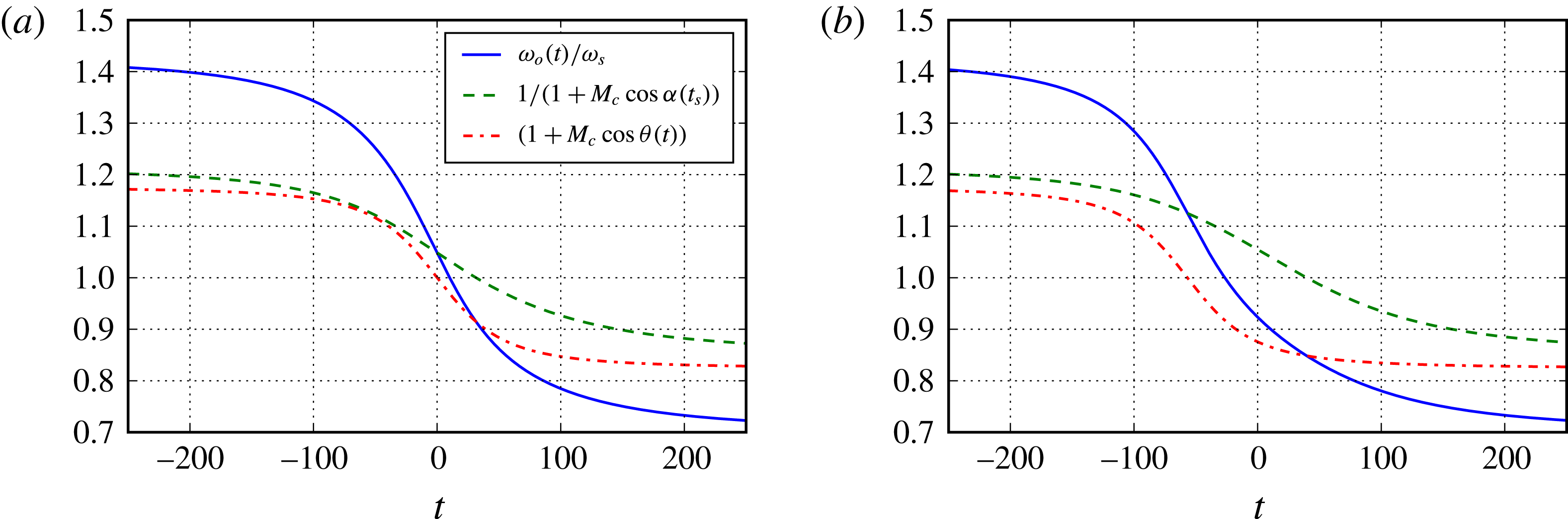
Figure 12 shows examples of the effective frequency
 $\unicode[STIX]{x1D714}_{o}$
together with the two separate Doppler shifts. Whereas for the plane wave the two Doppler shifts could cancel each other, with a point source their effects are compounded, resulting in a stronger deviation from the source frequency. From (4.3), we can see that the frequency shift will remain within the range
 $$\begin{eqnarray}\frac{-2M_{c}\unicode[STIX]{x1D714}_{s}}{1+M_{c}}\leqslant \unicode[STIX]{x1D714}_{o}-\unicode[STIX]{x1D714}_{s}\leqslant \frac{2M_{c}\unicode[STIX]{x1D714}_{s}}{1-M_{c}},\end{eqnarray}$$
corresponding to when the vortex is far downstream or far upstream respectively. The sidelobes due to the spectral broadening will be constrained to be within this frequency range.
The evolution of the normalised frequency
 $\unicode[STIX]{x1D714}_{o}/\unicode[STIX]{x1D714}_{s}$
for a source at
 $x_{s}=0$
and
 $y_{s}=-20L$
, with an observer at
 $y=10L$
and (a)
 $x=0$
or (b)
 $x=-10L$
. Here,
 $M_{c}=0.176$
.

4.2 Time-domain numerical model
The difference from § 3.2 is that the incoming sound field generated in the lower buffer zone now corresponds to a mass source obtained by adding the source terms
 $S/c_{\infty }^{2}$
and
 $S$
in (3.13a
) and (3.13c
) respectively. The source distribution is a time-harmonic point source,
 $S=\unicode[STIX]{x1D6FF}(\boldsymbol{x})\text{e}^{\text{i}\unicode[STIX]{x1D714}_{s}t}$
, with
 $\unicode[STIX]{x1D6FF}$
the Dirac delta function, and the theoretical expression for the sound field generated by this source can be given in terms of the velocity potential,
 $$\begin{eqnarray}\unicode[STIX]{x1D6F7}=\frac{\text{i}}{4\unicode[STIX]{x1D70C}_{\infty }c_{\infty }^{2}\sqrt{1-M_{c}^{2}}}\mathit{H}_{0}^{(2)}\left[k_{0}\frac{\sqrt{x^{2}+(1-M_{c}^{2})y^{2}}}{1-M_{c}^{2}}\right]\text{e}^{\text{i}(M_{c}/1-M_{c}^{2})k_{0}x+\text{i}\unicode[STIX]{x1D714}_{s}t}.\end{eqnarray}$$
This is used to obtain the corresponding velocity
 $\boldsymbol{u}^{\prime }=\unicode[STIX]{x1D735}\unicode[STIX]{x1D6F7}$
, pressure
 $p^{\prime }=-\unicode[STIX]{x1D70C}_{\infty }(\unicode[STIX]{x2202}/\unicode[STIX]{x2202}t+U_{c}\unicode[STIX]{x2202}/\unicode[STIX]{x2202}x)\unicode[STIX]{x1D6F7}$
and density
 $\unicode[STIX]{x1D70C}^{\prime }=p^{\prime }/c_{\infty }^{2}$
. It should be noted that it is the exact expressions for the pressure, velocity and density that are used in the buffer zone to impose the incoming sound field, and the point source itself is not part of the numerical model.
It is important to note that changing the mean flow velocity
 $M_{c}$
will also result in a change of directivity for the incident sound field. For instance, the variation in amplitude of the incident pressure field will vary with direction as
 $[1-M_{c}\cos (\unicode[STIX]{x1D711})/\unicode[STIX]{x1D70E}]/\sqrt{\unicode[STIX]{x1D70E}}$
, with
 $\unicode[STIX]{x1D70E}=[\cos ^{2}\unicode[STIX]{x1D711}+(1-M_{c}^{2})\sin ^{2}\unicode[STIX]{x1D711}]^{1/2}$
, where
 $\unicode[STIX]{x1D711}$
is the angle measured from the
 $x$
direction. This results in a significant increase (respectively decrease) of the sound field upstream (respectively downstream) of the source, which in turn influences the scattering by the convected vortex.
The same parameters as in § 3.2 are used to define the computational domain and the finite-difference grid.
4.3 The effects of the source frequency
The effect of the frequency, defined by the Helmholtz number
 $kL$
, is now assessed by considering a series of simulations for
 $kL=\unicode[STIX]{x03C0}/4,\unicode[STIX]{x03C0}/2,\unicode[STIX]{x03C0},2\unicode[STIX]{x03C0}$
and
 $4\unicode[STIX]{x03C0}$
. The source is located at
 $(x_{s},y_{s})=(0,-20L)$
. The mean flow velocity is
 $M_{c}=0.176$
and the vortex strength is
 $M_{v}=0.05$
.
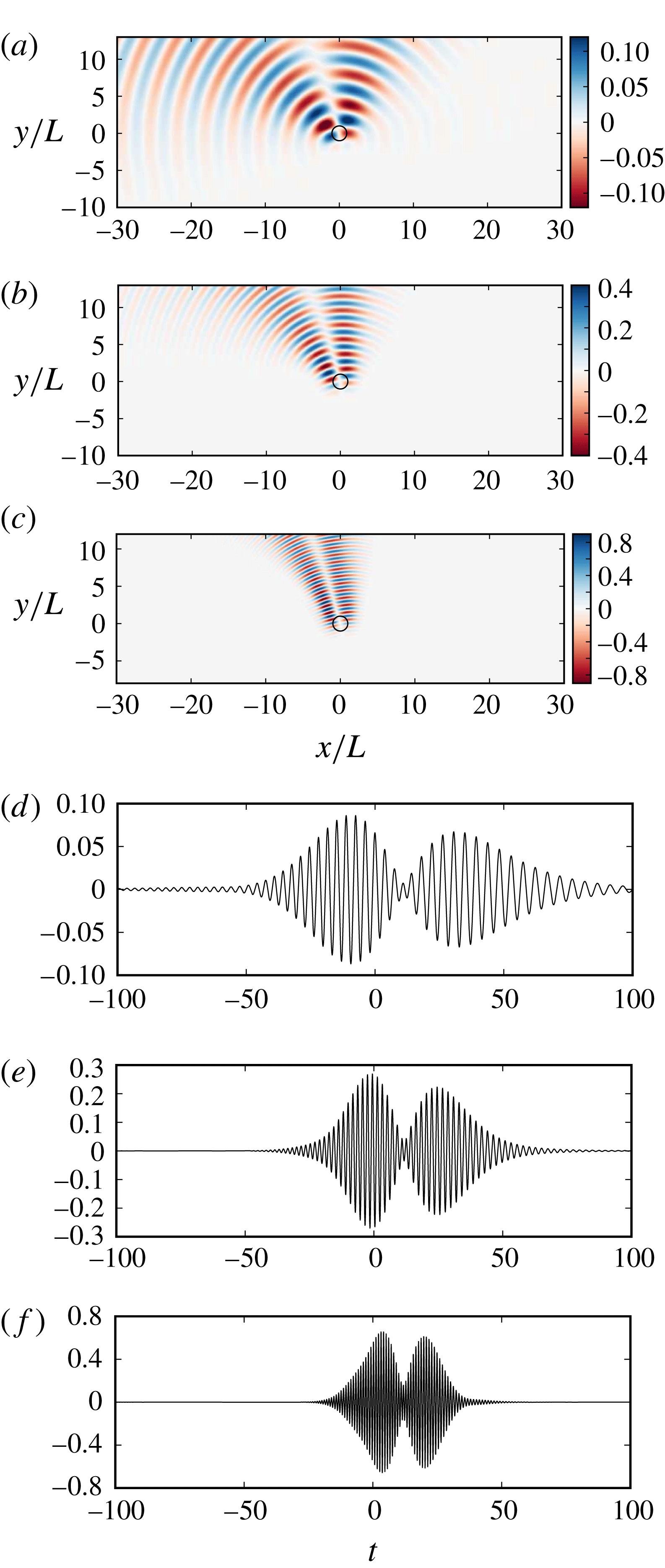
Figure 13 shows three examples of instantaneous pressure fields in the time-domain simulations for three different frequencies together with the pressure signals recorded just above the source at
 $(x,y)=(0,10L)$
. The corresponding spectra, also measured at
 $(x,y)=(0,10L)$
, are shown in figure 14. The time evolution of the pressure field during the passage of the vortex for the simulation with
 $kL=\unicode[STIX]{x03C0}/2$
is also presented in movie 2 as supplementary material.
The scattered pressure for different frequencies: (a,d)
 $kL=\unicode[STIX]{x03C0}/2$
, (b,e)
 $kL=\unicode[STIX]{x03C0}$
and (c,f)
 $kL=2\unicode[STIX]{x03C0}$
. (a–c) Scattered field at
 $t=0$
; (d–f) scattered pressure recorded at
 $x=0$
,
 $y=10L$
. Other parameters are
 $M_{c}=0.176$
,
 $M_{v}=0.05$
,
 $x_{s}=0$
and
 $y_{s}=-20L$
.

As already observed for the steady vortex in § 2.4, the strength of the scattered field increases with frequency. This increase of the scattering for shorter wavelengths is consistent with observations made in previous studies on the scattering by a turbulent shear layer (Candel et al. Reference Candel, Guédel and Julienne1975; Ewert et al. Reference Ewert, Kornow, Tester, Powles, Delfs and Rose2008; Kröber et al. Reference Kröber, Hellmold and Koop2013; McAlpine et al. Reference McAlpine, Powles and Tester2013; Sijtsma et al. Reference Sijtsma, Oerlemans, Tibbe, Berkefeld and Spehr2014).
Another trend clearly visible in figure 13(a–c) is that the two beams of the scattered field are narrower at high frequencies. This was also observed for the steady vortex in § 2.4. For the convected vortex, this translates into pressure signals in figure 13 formed of shorter wavepackets at high frequencies.
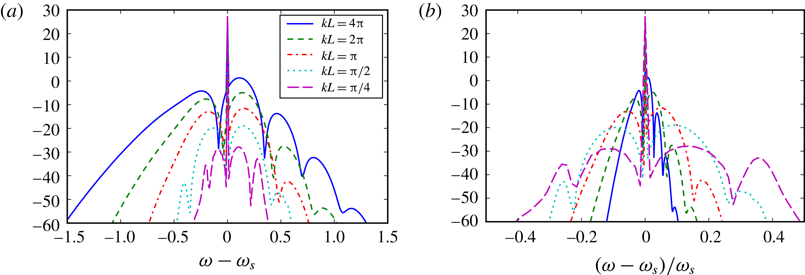
In figure 14(a), we can observe the evolution of the position of the sidebands, measured in terms of
 $\unicode[STIX]{x0394}\unicode[STIX]{x1D714}$
, the difference between the maximum of a sideband and the source frequency
 $\unicode[STIX]{x1D714}_{s}$
. The position of the main high-frequency sideband only varies slightly as the source frequency increases (except for the lowest source frequency). In contrast, the low-frequency sideband tends to move slightly away from the source frequency.
Based on the discussion in § 4.1 in terms of Doppler shifts, in particular (4.3)–(4.4), one would expect the position
 $\unicode[STIX]{x0394}\unicode[STIX]{x1D714}$
of the sideband to scale linearly with the source frequency. However, the results in figure 14(b), where the spectra are plotted against
 $(\unicode[STIX]{x1D714}-\unicode[STIX]{x1D714}_{s})/\unicode[STIX]{x1D714}_{s}$
, clearly show that this is not the case. This is explained by the change in the scattered field as the frequency increases, as discussed above and in § 2.4 for the steady vortex. When the source frequency is increased, the scattered beams narrow, and the wavepackets in figure 13 shorten. This implies that most of the scattered energy is received around
 $\tilde{\unicode[STIX]{x1D703}}=\tilde{\unicode[STIX]{x1D6FC}}$
, which, as shown by (4.3) and illustrated in figure 12, corresponds to small Doppler shifts. For the highest source frequencies, it can even be seen in § 2.4 that the main lobe of the scattered field overlaps the direction of the incident wave. As a result, the corresponding sideband on the spectrum (figure 14
a) is overlapping the peak at the source frequency. In conclusion, while increasing the source frequency results in a wider range of frequencies induced by the Doppler shifts, the scattered field is in fact perceived by the observer mostly at frequencies that are closer to the source frequency. These two opposite trends result in a weak dependence of
 $\unicode[STIX]{x0394}\unicode[STIX]{x1D714}$
on
 $\unicode[STIX]{x1D714}_{s}$
.
This illustrates the point that it is not sufficient to analyse the spectral broadening purely in terms of Doppler shift and that it is crucial to understand the scattering by the vortex in detail.
The previous studies on the scattering by a turbulent shear layer mentioned above observed that the source frequency mainly affects the levels and shapes of the sidebands on the spectra, but no effect on the position of their maxima is observed for the source frequencies considered. Since a shear layer is a continuous region of turbulence comprising many length scales, further work is required to fully recover all of the details of the scattering in such a configuration.
Sound pressure levels (in dB
 $/$
Hz ref. 1) of the total pressure fluctuation measured at
 $x=0$
,
 $y=10L$
for different frequencies as a function of (a) the frequency shift from the source frequency and (b) the relative frequency shift.

4.4 Effects of the convection velocity
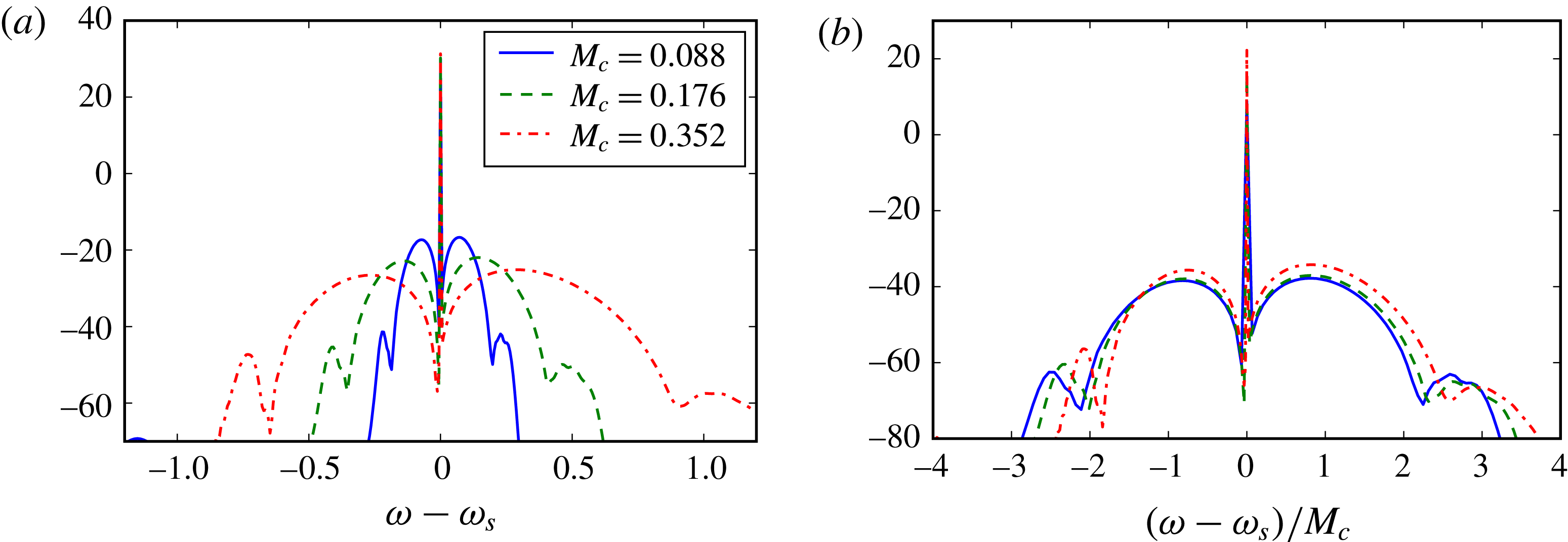
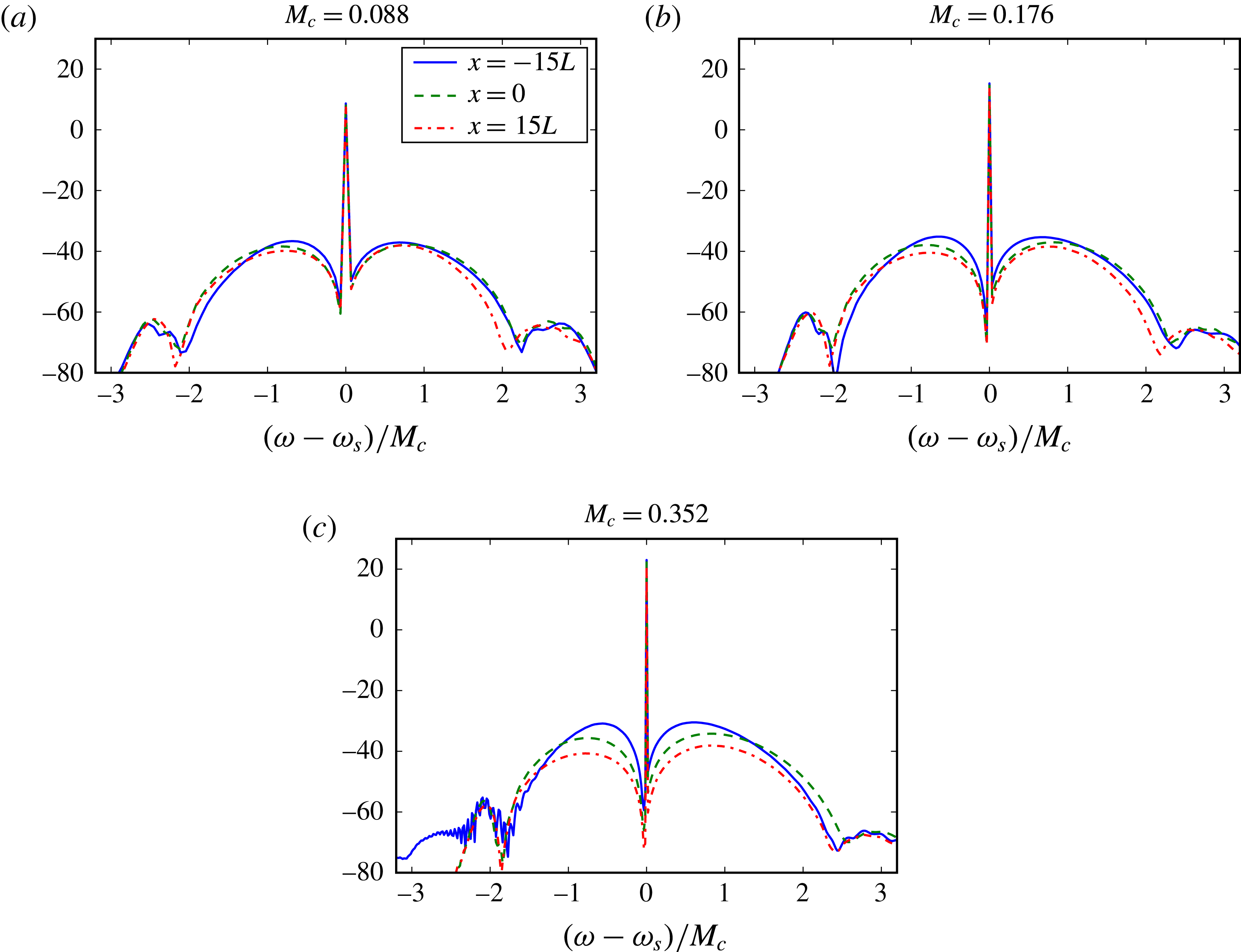
Finally, we consider the convection velocity, which has an important effect on the spectral broadening, since the Doppler shifts discussed in §§ 3.1 and 4.1 are directly controlled by the convection velocity
 $U_{c}$
.
Before we consider the case of the monopole, it is useful to revisit the case of the plane wave scattered by the vortex. In this situation, it is possible to identify the effect of the convection velocity more clearly. Starting from (3.8) for the signal measured by a fixed observer, we can define its Fourier transform as
 $$\begin{eqnarray}\hat{p}_{s}(\unicode[STIX]{x1D714})=\frac{1}{2\unicode[STIX]{x03C0}}\int \frac{D[\tilde{\unicode[STIX]{x1D703}}(t)-\unicode[STIX]{x1D6FC}]}{\sqrt{\tilde{r}(t)}}\exp \{\text{i}\unicode[STIX]{x1D714}_{v}[t-\tilde{r}(t)/c_{\infty }]-\text{i}\unicode[STIX]{x1D714}t\}\,\text{d}t.\end{eqnarray}$$
The difficulty with this expression is that
 $U_{c}$
is present in the definition of
 $\tilde{r}$
and
 $\tilde{\unicode[STIX]{x1D703}}$
. This can be avoided by formulating the integral in terms of the vortex position
 $x_{v}$
rather than the time
 $t$
. This yields
 $$\begin{eqnarray}\hat{p}_{s}(\unicode[STIX]{x1D714})=\frac{1}{2\unicode[STIX]{x03C0}U_{c}}\int \frac{D[\tilde{\unicode[STIX]{x1D703}}(x_{v})-\unicode[STIX]{x1D6FC}]}{\sqrt{\tilde{r}(x_{v})}}\exp \left[-\text{i}\frac{\unicode[STIX]{x1D714}_{v}}{c_{\infty }}\tilde{r}(x_{v})-\text{i}\frac{\unicode[STIX]{x1D714}-\unicode[STIX]{x1D714}_{v}}{U_{c}}x_{v}\right]\,\text{d}x_{v}.\end{eqnarray}$$
Since the expressions for
 $\tilde{r}(x_{v})$
and
 $\tilde{\unicode[STIX]{x1D703}}(x_{v})$
are independent of
 $U_{c}$
, the influence of this parameter is more apparent.
First, the factor
 $1/U_{c}$
indicates that the overall level of the scattered pressure will decrease for increased convection velocities. This is explained easily by noting that if the vortex is convected more rapidly past the observer, the latter will receive the scattered field for a shorter period of time.
Second, the convection velocity influences the frequency perceived by the vortex through the Doppler shift in (3.5). This will change the directivity and level of the scattered field through the dependence of
 $D$
on
 $\unicode[STIX]{x1D714}_{v}$
.
In the special case when
 $\unicode[STIX]{x1D6FC}=90^{\circ }$
, this Doppler shift is inexistent and we have
 $\unicode[STIX]{x1D714}_{v}=\unicode[STIX]{x1D714}_{s}$
. In this case, we can see that, when written as a function of
 $(\unicode[STIX]{x1D714}-\unicode[STIX]{x1D714}_{s})/U_{c}$
and scaled by
 $U_{c}$
, the spectrum becomes independent of
 $U_{c}$
. This has been verified using results from the time-domain numerical simulations. Given that the parameters are non-dimensional based on
 $L=1$
and
 $c_{\infty }=1$
, the quantity
 $\unicode[STIX]{x1D714}/U_{c}$
is proportional to the Strouhal number
 $fL/U_{c}$
. The fact that
 $(\unicode[STIX]{x1D714}-\unicode[STIX]{x1D714}_{s})/U_{c}$
is a relevant parameter follows from the expression
 $\unicode[STIX]{x1D714}_{o}=\unicode[STIX]{x1D714}_{v}(1+M_{c}\cos \tilde{\unicode[STIX]{x1D703}})$
for the Doppler shift between the vortex and the observer (see (3.9)). If
 $\unicode[STIX]{x1D714}_{v}=\unicode[STIX]{x1D714}_{s}$
, it is clear that the frequency shift will scale linearly with
 $U_{c}$
, thus resulting in wider sidebands for a higher convection velocity.
In the case of the monopole, the convection velocity influences several aspects of the problem. Increase of
 $U_{c}$
leads to a stronger Doppler shift between the source and the vortex, which results in a wider range of frequencies
 $\unicode[STIX]{x1D714}_{v}$
perceived by the vortex. As a result, the directivity and strength of the scattered field radiated by the vortex will vary more significantly as it moves past the observer. In addition, the Doppler shift from the vortex to the observer will also be more important.
Figure 15 shows a number of spectra for the scattered field for different convection velocities. The pressure signals are recorded over the same duration for the three velocities considered, corresponding to the time required for the vortex to travel through the computational domain at the lowest convection velocity (here,
 $M_{c}=0.088$
). When plotted as a function of the frequency shift
 $\unicode[STIX]{x1D714}-\unicode[STIX]{x1D714}_{s}$
, the two trends discussed above are apparent: when
 $U_{c}$
is increased, the overall levels of the sidebands decrease while their widths increase. When the levels are scaled by
 $U_{c}$
and the corresponding spectrum is plotted as a function of
 $(\unicode[STIX]{x1D714}-\unicode[STIX]{x1D714}_{s})/M_{c}$
, one obtains a good collapse of the data. The small differences visible in figure 15 can be attributed to convection effects on the incident sound field. This indicates that the simple scaling identified for the plane wave appears to be applicable, at least qualitatively, to a more complex sound field. In fact, it has been observed in several studies of the spectral broadening by turbulent shear layers that the width of the sidebands scales linearly with the convection velocity (Candel et al.
Reference Candel, Guédel and Julienne1975; Ewert et al.
Reference Ewert, Kornow, Tester, Powles, Delfs and Rose2008; Kröber et al.
Reference Kröber, Hellmold and Koop2013; McAlpine et al.
Reference McAlpine, Powles and Tester2013; Sijtsma et al.
Reference Sijtsma, Oerlemans, Tibbe, Berkefeld and Spehr2014), which is consistent with the present analysis. It should be noted that in these previous studies, as the amplitude of the turbulent fluctuations is scaling with the jet velocity, the levels of the sidebands on the spectra are also increasing with the jet velocity. In the present work, the vortex Mach number
 $M_{v}$
is kept constant for all of the convection velocities considered. An increase in the vortex Mach number would lead to changes in the levels and shapes of the scattered field, as discussed in § 2.4, resulting in turn in changes to the levels and shapes of the spectra.
While the results in figure 15 are for an observer just above the source, figure 16 illustrates the differences seen for other observer positions. For a small convection velocity
 $M_{c}=0.088$
, there is little variation between the three positions considered, apart from a small increase of the levels upstream of the source. However, the difference increases significantly as the convection velocity is increased, following the trend of larger sidebands upstream of the source and weaker sidebands downstream. This is explained by the change in the directivity of the incident sound field itself due to the convective amplification, which increases the amplitude of the sound upstream of the source (see § 4.2).
Sound pressure levels (in dB
 $/$
Hz ref. 1) of (a) the total pressure fluctuation and (b) the total pressure fluctuation scaled by
 $M_{c}$
measured at
 $x=0$
,
 $y=10L$
for different values of the convection velocity
 $M_{c}$
, plotted against (a) the frequency shift
 $\unicode[STIX]{x1D714}-\unicode[STIX]{x1D714}_{s}$
and (b) the Strouhal number
 $(\unicode[STIX]{x1D714}-\unicode[STIX]{x1D714}_{s})/M_{c}$
. Other parameters are
 $M_{v}=0.05$
and
 $kL=\unicode[STIX]{x03C0}/2$
.

Sound pressure levels (in dB
 $/$
Hz ref. 1) of the total pressure fluctuation measured at three different positions (all with
 $y=10L$
) and for different values of the convection velocity
 $M_{c}$
. It should be noted that the pressure amplitude has been scaled by
 $M_{c}$
. Other parameters are
 $M_{v}=0.05$
and
 $kL=\unicode[STIX]{x03C0}/2$
.

5 Conclusion
The scattering of a harmonic two-dimensional sound field by a single vortex has been studied in this paper to provide further insight into the mechanisms involved in the spectral broadening of the acoustic signal.
A semianalytical model has been formulated in the frequency domain for the scattering of a plane wave by a fixed vortex, and has been extended to the case where the vortex is convected by a uniform background flow. This model has been compared against, and supplemented by, a fully numerical approach in the time domain where the LEEs are solved using an unsteady base flow. This approach is capable of simulating cases with a moving vortex and more complex incident sound fields (the sound generated by a point mass source). Compared with previous analytical work, these two models are not restricted to asymptotic regimes (in terms of vortex strength or source frequency) and have provided a detailed parametric study of the spectral broadening. The results show the drastic changes in the shape and level of the scattered field between the low- and high-frequency regimes. In addition, the two models are able to capture the asymmetry in the scattered field, which is not predicted by analytical methods based on a low-frequency approximation.
Overall, the spectral broadening observed here stems from the combination of the spatial scattering of sound due to the refraction of waves propagating through the vortex, and two Doppler shifts induced by the motions of the vortex relative to the source and of the observer relative to the vortex.
The fact that the spectrum exhibits sidebands is directly explained by the directivity of the scattered field, which is composed of beams radiating from the vortex as it is convected past the observer. Each of these beams is perceived at frequencies above, or below, that of the sound source. Changes in the amplitude, width and shape of the sidebands can be explained by the interplay between the Doppler shifts (primarily governed by the convection velocity
 $M_{c}$
and the source frequency
 $\unicode[STIX]{x1D714}_{s}$
) and the amplitude and directivity of the scattered field from the vortex (controlled by the Helmholtz number
 $kL$
and the vortex strength
 $M_{v}$
).
For instance, it has been observed in measured data that the position of the sidebands does not vary significantly with the source frequency. In the present results, a weak dependence of the position of the sidebands on the source frequency is shown to be the result of two competing effects: the Doppler shifts lead to an increase of the sideband width when the source frequency is increased, whereas the scattered beams radiated from the vortex become narrower, which results in a reduction of the sideband width. Further work is required to explain the absence of such a dependence of the position of the sidebands on the source frequency in existing experimental results on the scattering by a shear layer.
Another trend also found in measurements and models for a region of turbulence is that the sideband width scales linearly with the convection velocity. This is also observed with a single vortex and can be explained in terms of the Doppler shifts.
Additionally, the scattering from the vortex studied here was found to conserve the acoustic energy, and it was confirmed that the inhomogeneities in pressure and density in the base flow due to the vortex are not significant for the spectral broadening.
While the role of a Doppler shift has been considered in previous work to justify spectral broadening, the present work shows that a better understanding of the scattering by a single vortex (as described in § 2) can provide further details on the underlying mechanisms. It is also striking that a number of features and trends of haystacking from a region of turbulence are recovered when considering a single vortex, which allows for a detailed analysis to explain some of the causes and properties of the spectral broadening.
Finally, it should be noted that in all of the cases considered here, the amplitude of the original tone is not significantly modified by the scattering. This is because a single vortex, even with a large induced velocity
 $M_{v}$
, is only affecting a small portion of the time signals recorded. Thus, overall, the initial amplitude of the tone remains almost unchanged if the time signals are long enough. It is necessary to consider a region of turbulence, composed of a large number of vortices scattering at all time, to observe a noticeable reduction of the tone.
The next logical step is to perform a similar study with a region of turbulence. This work is ongoing in two dimensions using a stochastic method to generate turbulent velocity fields with different length scales, time scales and energy spectra. Preliminary results indicate that the trends and physical processes discussed in the present paper remain relevant when considering a region of turbulence (Clair & Gabard Reference Clair and Gabard2016). A number of postprocessing techniques can also be applied to isolate the physical mechanisms responsible for the spectral broadening. These results will be reported in a subsequent communication. Ultimately, three-dimensional effects should be investigated. The directivity of the scattered field will be affected by the three-dimensional shape of the vortex considered (e.g. a vortex filament or a compact vortex), which will in turn affect the spectral broadening.
Acknowledgements
This work was partly supported by Rolls-Royce plc through the University Technology Center in Gas Turbine Noise at the University of Southampton and funded by EPSRC grant EP/K017551/1. Part of this work was also performed within the framework of the Labex CeLyA of the Université de Lyon, within the programme ‘Investissements d’Avenir’ (ANR-10-LABX-0060/ANR-11-IDEX-0007) operated by the French National Research Agency (ANR). The authors would like to acknowledge the members of the AS/TA department of DLR for providing the PIANO solver. The authors also acknowledge the use of the IRIDIS High Performance Computing Facility, and associated support services, at the University of Southampton in the completion of this work. All data supporting this study are openly available at https://doi.org/10.5281/zenodo.1147439.
Supplementary movies
Supplementary movies are available at https://doi.org/10.1017/jfm.2018.94.
Appendix A. Derivation of (2.13)
Using the decomposition of the incident plane wave in terms of Bessel functions given in (2.11), the total pressure can be written as
 $$\begin{eqnarray}p^{\prime }=\mathop{\sum }_{m=-\infty }^{+\infty }\{\text{i}^{-m}P\text{J}_{m}(kr)+A_{m}\mathit{H}_{m}^{(2)}(kr)\}\text{e}^{-\text{i}m\unicode[STIX]{x1D703}}.\end{eqnarray}$$
The corresponding expression for the radial acoustic velocity is
 $$\begin{eqnarray}u_{r}^{\prime }=\frac{\text{i}}{\unicode[STIX]{x1D70C}_{\infty }c_{\infty }}\mathop{\sum }_{m=-\infty }^{+\infty }\{\text{i}^{-m}P\text{J}_{m}^{\prime }(kr)+A_{m}\mathit{H}_{m}^{(2)\prime }(kr)\}\text{e}^{-\text{i}m\unicode[STIX]{x1D703}}.\end{eqnarray}$$
Upon introducing these expressions into (2.12), the acoustic power can be written as the sum of three terms,
 $W_{t}=W_{i}+W_{s}+W_{si}$
. The first term,
 $W_{i}$
, corresponds to the acoustic power of the plane wave alone, which vanishes as expected,
 $$\begin{eqnarray}W_{i}=\frac{\unicode[STIX]{x03C0}r}{\unicode[STIX]{x1D70C}_{\infty }c_{\infty }}|P|^{2}\mathop{\sum }_{m=-\infty }^{+\infty }\text{Re}\{\text{i}\text{J}_{m}(kr)\text{J}_{m}^{\prime }(kr)\}=0.\end{eqnarray}$$
The second term,
 $W_{s}$
, corresponds to the power of the scattered field taken in isolation,
 $$\begin{eqnarray}W_{s}=\frac{\unicode[STIX]{x03C0}r}{\unicode[STIX]{x1D70C}_{\infty }c_{\infty }}\mathop{\sum }_{m=-\infty }^{+\infty }|A_{m}|^{2}\text{Re}\{\text{i}\mathit{H}_{m}^{(2)}(kr)^{\ast }\mathit{H}_{m}^{(2)\prime }(kr)\}.\end{eqnarray}$$
Using the definition
 $\mathit{H}_{m}^{(2)}(z)=\text{J}_{m}(z)-\text{i}\mathit{Y}_{m}(z)$
, we can write
 $$\begin{eqnarray}\text{Re}\{\text{i}\mathit{H}_{m}^{(2)}(z)^{\ast }\mathit{H}_{m}^{(2)\prime }(z)\}=\text{J}_{m}(z)\mathit{Y}_{m}^{\prime }(z)-\text{J}_{m}^{\prime }(z)\mathit{Y}_{m}(z)=\frac{2}{\unicode[STIX]{x03C0}z},\end{eqnarray}$$
where the last equality is a result for the Wronskian between
 $\text{J}_{m}(z)$
and
 $\mathit{Y}_{m}(z)$
; see equation (9.1.16) in Abramowitz & Stegun (Reference Abramowitz and Stegun1964). This last equation leads directly to the first expression in (2.13).
The third term,
 $W_{si}$
, is a contribution to the total acoustic power from the interference between the incident plane wave and the scattered field,
 $$\begin{eqnarray}W_{si}=\frac{\unicode[STIX]{x03C0}r}{\unicode[STIX]{x1D70C}_{\infty }c_{\infty }}\mathop{\sum }_{m=-\infty }^{+\infty }\text{Re}\{\text{i}^{1+m}P^{\ast }A_{m}\text{J}_{m}(kr)\mathit{H}_{m}^{(2)\prime }(kr)+\text{i}^{1-m}PA_{m}^{\ast }\text{J}_{m}^{\prime }(kr)\mathit{H}_{m}^{(2)\ast }(kr)\}.\end{eqnarray}$$
We can use the following result for the Wronskian between
 $\text{J}_{m}(z)$
and
 $\mathit{H}_{m}^{(2)}(z)$
:
 $$\begin{eqnarray}\text{J}_{m}(z)\mathit{H}_{m}^{(2)\prime }(z)-\text{J}_{m}^{\prime }(z)\mathit{H}_{m}^{(2)}(z)=\frac{-2\text{i}}{\unicode[STIX]{x03C0}z},\end{eqnarray}$$
to write
 $$\begin{eqnarray}\displaystyle W_{si} & = & \displaystyle \frac{\unicode[STIX]{x03C0}r}{\unicode[STIX]{x1D70C}_{\infty }c_{\infty }}\mathop{\sum }_{m=-\infty }^{+\infty }\text{Re}\left\{\vphantom{\frac{2\text{i}^{m}}{\unicode[STIX]{x03C0}kr}}\text{i}^{1+m}P^{\ast }A_{m}\text{J}_{m}(kr)\mathit{H}_{m}^{(2)\prime }(kr)\right.\nonumber\\ \displaystyle & & \displaystyle \left.+\,\text{i}^{1-m}PA_{m}^{\ast }\text{J}_{m}(kr)\mathit{H}_{m}^{(2)\prime }(kr)^{\ast }+P^{\ast }A_{m}\frac{2\text{i}^{m}}{\unicode[STIX]{x03C0}kr}\right\}.\end{eqnarray}$$
The sum of the first two terms in the brackets is imaginary and it follows that only the last term remains. The expression can then be simplified to yield the second expression in (2.13).
Appendix B. Influence of
 $p_{t}$
and
$\unicode[STIX]{x1D70C}_{t}$


The hypothesis that
 $p_{t}$
and
 $\unicode[STIX]{x1D70C}_{t}$
have no significant influence can be assessed by using the semianalytical model presented in § 2.2, where these terms are retained. Figure 17 shows the directivity of the scattered field for a steady vortex given by (3.12) or by (3.12a
) and
 $\unicode[STIX]{x1D70C}=\unicode[STIX]{x1D70C}_{\infty }$
and
 $p=p_{\infty }$
. It can be seen that the influence of the non-uniform pressure and density in the base flow has very little impact on the scattered field. This has been verified for a range of frequencies (up to
 $kL=8\unicode[STIX]{x03C0}$
) and vortex strengths (up to
 $M_{v}=0.25$
). Therefore, the effect of
 $p_{t}$
and
 $\unicode[STIX]{x1D70C}_{t}$
will be ignored in the numerical model.
It should be noted that for a flow with significant turbulent temperature fluctuations (hot spots), this assumption does not hold as hot spots are known to contribute to scattering.
This simplification was used since the PIANO solver used here allows us to consider an unsteady base flow, but only for the velocity field. Previous work (Ewert et al. Reference Ewert, Kornow, Tester, Powles, Delfs and Rose2008, Reference Ewert, Kornow, Delfs, Yin, Röber and Rose2009) considered that for a non-heated turbulent flow, such as a cold jet, the scattering was mostly induced by the unsteady velocity fluctuations, while the effect of density and pressure fluctuations was deemed to be negligible.
The change in directivity
 $D(\unicode[STIX]{x1D703})$
due to the approximation
 $\unicode[STIX]{x1D70C}=\unicode[STIX]{x1D70C}_{\infty }$
and
 $p=p_{\infty }$
for the base flow. The parameters are
 $kL=4\unicode[STIX]{x03C0}$
and
 $M_{v}=0.25$
.