2.1. ROV model

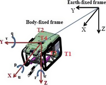
A typical ROV, as illustrated in Fig. 1, utilizes four thrusters to generate the force and torque necessary for motion. The motion of an ROV in 6-DOF can be represented in a vectorial form through the use of the SNAME notation (SNAME 1950) outlined in Table I; this notation generalizes six individual coordinates to describe the position and orientation, as well as the linear and angular velocities of the vehicle.

Figure 1.

An ROV with two coordinate systems [Reference Hosseini and Seyedtabaii2].

Table I.

The SNAME notation for ROV.

In the local body-fixed reference frame (b-frame), a nonlinear dynamic model of an ROV is defined by refs. [Reference Hosseini and Seyedtabaii2, Reference Hoang and Kreuzer17]:

(1) \begin{equation} M\dot{v}+C(v)v+D(v)v+g(v)=\tau (v_{a})+d \end{equation}

with:

\begin{align*} v&=\left[\textrm{u}\,\textrm{v}\,\textrm{w}\,\textrm{p}\,\textrm{q}\,\textrm{r}\right]^{T}\!,\\ M&=M_{RB}+M_{A},\\ C\!\left(v\right)&=C_{RB}\!\left(v\right)+C_{A}\!\left(v\right) \end{align*}

In Eq. (1), $v$ is the velocity vector in a body-fixed reference frame, consisting of the three linear velocities $[\textrm{u}\ \ \textrm{v}\ \ \textrm{w}]$ in the three axis, as well as the angular rates of the ROV. $d$ disturbances caused by underwater currents, $\tau (v_{a})$ represents the forces and torques that act upon the ROV, and the voltage $v_{a}$ explains the control signal applied to the thruster.

The parameter $M\in \mathbb{R}^{6\times 6}$ is the inertia matrix that includes the added mass and the rigid-body mass matrix, $C\in \mathbb{R}^{6\times 6}$ is the Coriolis matrix and the centripetal terms, and $D\in \mathbb{R}^{6\times 6}$ is the added mass and damping matrix. Finally, the gravity vector, which contains both weight and buoyancy, is represented by $g(\eta )$ . The matrices $M_{A}, C_{A}(v)$ represent hydrodynamic added mass and Coriolis acceleration, $M_{RB}$ is the rigid-body mass matrix, and $C_{RB}$ is the rigid-body Coriolis and centripetal matrix [Reference Hosseini and Seyedtabaii2].

For a port-starboard symmetrical vehicle with homogenous mass distribution, CG satisfying $y_{g}=0$ and products of inertia $I_{xy}=I_{yz}=0$ , the system inertia matrix becomes

(2) \begin{equation} M=\left[\begin{array}{c@{\quad}c@{\quad}c@{\quad}c@{\quad}c@{\quad}c} m-X_{\dot{u}} & 0 & -X_{\dot{w}} & 0 & mz_{g}-X_{\dot{q}} & 0\\[3pt] 0 & m-Y_{\dot{v}} & 0 & -mz_{g}-Y_{\dot{p}} & 0 & mx_{g}-Y_{\dot{r}}\\[3pt] -X_{\dot{w}} & 0 & m-Z_{\dot{w}} & 0 & -mx_{g}-Z_{\dot{q}} & 0\\[3pt] 0 & -mz_{g}-Y_{\dot{p}} & 0 & I_{x}-K_{\dot{p}} & 0 & -I_{zx}-K_{\dot{r}}\\[3pt] mz_{g}-X_{\dot{q}} & 0 & -mx_{g}-Z_{\dot{q}} & 0 & I_{y}-M_{\dot{q}} & 0\\[3pt] 0 & mx_{g}-Y_{\dot{r}} & 0 & -I_{zx}-K_{\dot{r}} & 0 & I_{z}-N_{\dot{r}} \end{array}\right] \end{equation}

The Coriolis and centripetal matrices are defined as:

(3) \begin{equation} C_{A}\!\left(v\right)=\left[\begin{array}{c@{\quad}c@{\quad}c@{\quad}c@{\quad}c@{\quad}c} 0 & 0 & 0 & 0 & -a_{3} & a_{2}\\[3pt] 0 & 0 & 0 & a_{3} & 0 & -a_{1}\\[3pt] 0 & 0 & 0 & -a_{2} & a_{1} & 0\\[3pt] 0 & -a_{3} & a_{2} & 0 & 0 & b_{2}\\[3pt] a_{3} & 0 & -a_{1} & b_{3} & -b_{3} & -b_{1}\\[3pt] -a_{2} & a_{1} & 0 & -b_{2} & b_{1} & 0 \end{array}\right] \end{equation}

where

(4) \begin{align} a_{1} & =X_{\dot{u}}u+X_{\dot{w}}w+X_{\dot{q}}q\nonumber\\[3pt] a_{2} & =Y_{\dot{v}}v+Y_{\dot{p}}p+Y_{\dot{r}}r\nonumber\\[3pt] a_{3} & =Z_{\dot{u}}u+Z_{\dot{w}}w+Z_{\dot{q}}q\\[3pt] b_{1} & =K_{\dot{v}}v+K_{\dot{p}}p+K_{\dot{r}}r\nonumber\\[3pt] b_{2} & =M_{\dot{u}}u+M_{\dot{w}}w+M_{\dot{q}}q\nonumber\\[3pt] b_{3} & =N_{\dot{v}}v+N_{\dot{p}}p+N_{\dot{r}}r \nonumber\end{align}

and

(5) \begin{equation} C_{RB}\!\left(v\right)=\left[\begin{array}{c@{\quad}c@{\quad}c@{\quad}c@{\quad}c@{\quad}c} 0 & -mr & mq & mz_{g}r & -mx_{g}q & -mx_{g}r\\[3pt] mr & 0 & -mp & 0 & m\!\left(z_{g}r+x_{g}p\right) & 0\\[3pt] -mq & mp & 0 & -mz_{g}p & -mz_{g}q & mx_{g}p\\[3pt] -mz_{g}r & 0 & mz_{g}p & 0 & -I_{xz}p+I_{z}r & -I_{y}q\\[3pt] mx_{g}q & -m\!\left(z_{g}r+x_{g}p\right) & mz_{g}q & I_{xz}p-I_{z}r & 0 & -I_{xz}r+I_{x}p\\[3pt] mx_{g}r & 0 & -mx_{g}p & I_{y}q & I_{xz}r-I_{x}p & 0 \end{array}\right] \end{equation}

Linear damping for a port-starboard symmetrical vehicle takes the following form:

(6) \begin{equation} D=-\left[\begin{array}{c@{\quad}c@{\quad}c@{\quad}c@{\quad}c@{\quad}c} X_{u} & 0 & X_{w} & 0 & X_{q} & 0\\[3pt] 0 & Y_{v} & 0 & Y_{p} & 0 & Y_{r}\\[3pt] Z_{u} & 0 & Z_{w} & 0 & Z_{q} & 0\\[3pt] 0 & K_{v} & 0 & K_{p} & 0 & K_{r}\\[3pt] M_{u} & 0 & M_{w} & 0 & M_{q} & 0\\[3pt] 0 & N_{v} & 0 & N_{p} & 0 & N_{r} \end{array}\right] \end{equation}

The relationship between velocity in the body and the earth-fixed coordinate is represented by,

(7) \begin{equation} \dot{\eta }=J(\eta )v \end{equation}

where $J(\eta )$ is the transformation matrix between the body-fixed and the earth-fixed frame. In Eq. (1), $\eta =[x,y,z,\phi,\theta,\psi ]$ is the earth frame state vector containing position $(\textrm{X},\textrm{Y},\textrm{Z})$ and attitude (roll, pitch, and yaw angles) [Reference Salgado-Jiménez, García-Valdovinos, Delgado-Ramírez and Bartoszewicz18]. Therefore, a model of a ROV in the earth frame is defined as follows [Reference Hosseini and Seyedtabaii2, Reference Koh, Lau, Low, Seet, Swei and Cheng19]:

(8) \begin{equation} M_{\eta }(\eta )\ddot{\eta }+C_{\eta }(\eta,v)\dot{\eta }+D_{\eta }(\eta,v)\dot{\eta }+g_{\eta }(\eta )=\tau _{\eta } \end{equation}

where

\begin{align*} M_{\eta }&=J^{-T}\!\left(\eta \right)MJ^{-1}\!\left(\eta \right)\\ C_{\eta }\!\left(\eta,\nu \right)&=J^{-T}\!\left(\eta \right)\left[C\!\left(\nu \right)-MJ^{-1}\!\left(\eta \right)J\!\left(\eta \right)\right]J^{-1}\!\left(\eta \right)\\ D_{\eta }\!\left(\eta,\nu \right)&=J^{-T}\!\left(\eta \right)D\!\left(\nu \right)J^{-1}\!\left(\eta \right)\\ g_{\eta }\!\left(\eta \right)&=J^{-T}\!\left(\eta \right)g\!\left(\eta \right)\\ \tau _{\eta }\!\left(\eta \right)&=J^{-T}\!\left(\eta \right)\tau \!\left(v_{a}\right) \end{align*}

2.2. Thruster

The applied force and torque vector $\tau$ are defined in Eq. (1) in the body-fixed coordinate frame. According to Eq. (9), this vector depends on the produced torque by each of the four thrusters. Elements of matrix B indicate the position of the ROV’s propulsions relative to its center of gravity.

(9) \begin{equation} \tau =\left[\begin{array}{l} X\\[3pt] Y\\[3pt] Z\\[3pt] K\\[3pt] M\\[3pt] N \end{array}\right]=BT\!\left(v_{a}\right)=\left[\begin{array}{c@{\quad}c@{\quad}c@{\quad}c} 1 & 1 & 0 & 0\\[3pt] 0 & 0 & 1 & 0\\[3pt] 0 & 0 & 0 & 1\\[3pt] 0 & 0 & -z_{F3} & y_{F4}\\[3pt] z_{F1} & z_{F2} & 0 & -x_{F4}\\[3pt] -y_{F1} & -y_{F2} & x_{F3} & 0 \end{array}\right]\left[\begin{array}{l} T_{1}\\[3pt] T_{2}\\[3pt] T_{3}\\[3pt] T_{4} \end{array}\right] \end{equation}

As shown in Fig. 1, the ROV is equipped with four DC motors acting as thrusters. To manage longitudinal movement, $T_{1}, T_{2}$ at the end, $T_{3}$ for the lateral movement and $T_{4}$ for diving and vertical climbing have been installed.

The thruster model is defined by the hydrodynamic model of the propeller and the characteristics of the DC motor. Newtonian fluid mechanics can be used to define a hydrodynamic model of the propeller [Reference Koh, Lau, Low, Seet, Swei and Cheng19]:

(10) \begin{equation} T=K_{T0}\dot{\omega }+K_{T}| \omega | \omega \end{equation}

where $T$ denotes the propeller thrust, $\omega$ denotes thruster rotational speed, $K_{T0}, K_{T}$ denote thruster coefficients, and thruster coefficients, and these values are equivalent to refs. [Reference Wan and Wang20, Reference Aras, Abdullah, Rahman and Aziz21]:

(11) \begin{equation} K_{T}=k_{t}\rho D^{4} \end{equation}

In Eq. (11), $k_{t}$ is a constant value, $\rho$ denotes the water density, and $D$ denotes the diameter of the propeller (in meters). The armature voltage $(v_{a})$ applied to motors is converted to ROV propulsion using an electromechanical model of the motor:

(12) \begin{equation} v_{a}=R_{a}i_{a}+L_{a}i_{a}+k_{b}\omega \end{equation}

where $i_{a}$ is the armature current, $\omega$ represents the rotor rotation speed, and the Ohmic resistance, inductance, and the tacho constant are denoted, respectively, as $R_{a}, L_{a}$ , and $k_{a}$ . The motor’s electric torque is determined by:

(13) \begin{equation} T=k_{m}i_{a} \end{equation}

Assuming the inductance of the armature circuit $(L_{a})$ in Eq. (12) is negligible, the equation can be rewritten as:

(14) \begin{equation} \nu _{a}=R_{a}i_{a}+k_{b}\omega \end{equation}

Since the propeller’s rotational speed is constant, the rate of speed $K_{T0}$ in Eq. (10) can be omitted and the equation rewritten as follows [Reference Koh, Lau, Low, Seet, Swei and Cheng19]:

(15) \begin{equation} T=K_{T}\!\left| \omega \right| \omega \end{equation}

The propeller’s rotational speed is equivalent to:

(16) \begin{equation} \omega =\sqrt{\frac{T}{K_{T}}} \end{equation}

Eqs. (14) and (16) are substituted in Eq. (14) ref. [Reference Aras, Abdullah, Rahman and Aziz21]:

(17) \begin{equation} v_{a}=R_{a}\frac{T}{k_{m}}+k_{b}\sqrt{\frac{T}{K_{T}}} \end{equation}

3.1. Control design

The left-hand side of Eq. (8) is linearly parametrizable by the product of a regressor $Y(\eta,\dot{\eta },\ddot{\eta })\in R^{n\times p}$ with a vector $\theta \in R^{p}$ that includes unknown constant parameters. The parametrization $Y(\eta,\dot{\eta },\ddot{\eta })\theta$ can be rewritten according to the nominal reference $\dot{\eta }_{r}$ and its derivative:

(18) \begin{equation} M_{\eta }(\dot{\eta })\ddot{\eta }_{r}+C_{\eta }(\eta,v)\dot{\eta }_{r}+D_{\eta }(\eta,v)\dot{\eta }_{r}+g_{\eta }(\eta )=Y(\eta,\dot{\eta },\eta _{r},\dot{\eta }_{r})\theta \end{equation}

Substituting Eq. (18) into Eq. (8) yields the open-loop error dynamics in error coordinates $s_{r}=\dot{\eta }-\dot{\eta }_{r}$ as follows:

(19) \begin{equation} M_{\eta }(\dot{\eta })\dot{s}_{r}+\left \{C_{\eta }(\eta,v)+D_{\eta }(\eta,v)\right \}s_{r}=\tau _{\eta }-\dot{\eta }_{r}Y(\eta,\dot{\eta },\eta _{r},\dot{\eta }_{r})\theta \end{equation}

An aim of designing a controller for open-loop error dynamics Eq. (19) is to determine $\tau _{\eta }$ such that an exponential convergence is guaranteed. This will be accomplished without knowledge of system dynamics and high-frequency components. Let us define dynamic reference as a function of ( $\dot{\eta }_{d}, \tilde{\eta }, s_{\eta }$ ) as follows [Reference Parra-Vega, Arimoto, Liu, Hirzinger and Akella22]:

(20) \begin{equation} \dot{\eta }_{r}=\dot{\eta }_{d}-\alpha \tilde{\eta }+s_{d}-\gamma \int _{0}^{t}\text{sign}(s_{\eta })d\sigma \end{equation}

where $\tilde{\eta }=\eta -\eta _{d}$ is the position tracking error. $\eta _{d}$ indicates the desired path, $\alpha$ and $\gamma$ are positive definite $(n\times n)$ gain matrices, $\text{sign}(s_{\eta })$ is the discontinuous function signum of vector $s_{\eta }$ , and:

(21) \begin{equation} s=\dot{\tilde{\eta }}+\alpha \tilde{\eta },{\ } s_{d}=s(t_{0})e^{-kt},{\ } s_{\eta }=s-s_{d} \end{equation}

where $k\gt 0$ , substituting Eq. (20) into the extended error $s_{r}=\dot{\eta }-\dot{\eta }_{r}$ leads to refs. [Reference Parra-Vega, Arimoto, Liu, Hirzinger and Akella22, Reference Parra-Vega and Arimoto23]:

(22) \begin{equation} s_{r}=s_{\eta }+\gamma \int _{0}^{t}\text{sign}(s_{\eta })d\sigma \end{equation}

This surface yields fast asymptotic convergence with a certain degree of robustness.

The control signal of the ROV model Eq. (8) in the closed loop is defined as follows [Reference Parra-Vega, Arimoto, Liu, Hirzinger and Akella22]:

(23) \begin{equation} \tau _{\eta }=-K_{d}s_{r} \end{equation}

where $K_{d}$ is a diagonal positive $n\times n$ matrix, which is called the feedback gain.

3.2. The stability analyses

A structural feature of Eqs. (1) and (20) is expressed by fixed-parameter $\beta _{i}(i=0,1,\ldots )$ , which will be used in the proof of stability:

(24) \begin{equation} \begin{split} \| M_{\eta }\| &\geq \lambda _{m}(M_{\eta })\gt \beta _{0}\gt 0, \\ \| M_{\eta }\| &\leq \lambda _{M}(M_{\eta })\lt \beta _{1}\lt \infty, \\ \| C_{\eta }\| &\leq \beta _{2}\| \dot{\eta }\|,\\ \| g_{\eta }\| &\leq \beta _{3}, \\ \| \dot{\eta }_{r}\| &\leq \alpha \| \dot{\eta }\| +\gamma \| \sigma \| +\beta _{4}, \\ \| \ddot{\eta }_{r}\| &\leq \alpha \| \dot{\tilde{\eta }}\| +\beta _{5} \end{split} \end{equation}

where $\lambda _{m}(M_{\eta })$ and $\lambda _{M}(M_{\eta })$ stand for minimum and maximum matrix eigenvalues, $M\in R^{n\times n}$ , respectively. Constants $\beta _{i}$ can be computed from the states of the system, desired trajectory, feedback gains, and a conservative upper bound of the dynamic model of the ROV. Using Eq. (24) and Eq. (18) becomes

(25) \begin{equation} \begin{split} Y(\eta,\dot{\eta },\ddot{\eta })\theta &\leq \| M_{\eta }(\dot{\eta })\| \| \ddot{\eta }_{r}\| +(\| C_{\eta }(\eta,v)\| +\| D_{\eta }(\eta,v)\| ) \\ & \quad \times \| \dot{\eta }_{r}\| +\| g_{\eta }(\eta )\| \\ &\leq \beta _{1}\alpha \| \dot{\tilde{\eta }}\| +(\beta _{2}\| \dot{\eta }\| +\lambda _{M}(D_{\eta })) \\&\quad \times (\alpha \| \tilde{\eta }\| +\gamma \| \sigma \| +\beta _{4})+\overline{\beta } \\ &=\rho (t) \end{split} \end{equation}

where $\overline{\beta }=\beta _{1}\beta _{5}+\beta _{3}$ . Furthermore, $\rho (t)=f(\eta,\dot{\eta },\dot{\eta }_{r},\ddot{\eta }_{r})$ is a function of state variables.

1. Closed-loop convergence

Replacement of Eq. (23) into Eq. (19) leads to the following closed-loop error dynamic:

(26) \begin{equation} M_{\eta }(\dot{\eta })\dot{s}_{r}=-(C_{\eta }(\eta,v)+K)s_{r}-Y(\eta,\dot{\eta },\eta _{r},\dot{\eta }_{r})\theta \end{equation}

where $K=D_{\eta }(v,\eta )+K_{d}$ candidate a Lyapunov function as ref. [Reference Parra-Vega, Arimoto, Liu, Hirzinger and Akella22]:

(27) \begin{equation} V=\frac{1}{2}s_{r}^{T}M_{\eta }\!\left(\eta \right)s_{r} \end{equation}

Substituting the derivative of the Lyapunov function in Eq. (27) together with using Eq. (26) becomes

(28) \begin{equation} \begin{split} \dot{V}&=-s_{r}^{T}Ks_{r}-s_{r}^{T}Y_{r}\theta \\ &\leq -s_{r}^{T}Ks_{r}-\| s_{r}\| \| Y_{r}\theta \| \\ &\leq -\| K_{1}s_{r}\| ^{2}-\| s_{r}\| \rho (t) \end{split} \end{equation}

where $K=K_{1}^{T}K_{1}$ . Since $s_{r}$ is a function of $\tilde{\eta }, \dot{\tilde{\eta }}, \sigma$ and the initial conditions, then in the presence of small initial errors belonging to a finite set $\varepsilon$ with radius $r$ centered in the equilibrium point $s_{r}=0$ , and by invoking Lyapunov arguments, there exists a large enough gain $K_{d}$ (remember that $K=D_{\eta }(v,\eta )+K_{d}=K_{1}^{T}K_{1}$ ), such that $s_{r}$ converges to a finite set $\varepsilon$ . Then, the boundedness of tracking error is guaranteed $s_{r}\rightarrow \varepsilon\ as\ t\rightarrow \infty$ .

As a result, $s_{r}$ is bounded by a constant $\varepsilon _{r}$ . Boundedness of $s_{r}$ indicates that the closed-loop system mode is convergent. There exists an upper bound $\overline{\rho }$ where $\overline{\rho }\geq \rho (t)$ . Since the positive definite matrix $M$ is bounded, the boundedness of $\dot{s}_{r}$ in Eq. (29) is achieved.

(29) \begin{equation} \begin{split} \dot{s}_{r}&=-M_{\eta }^{-1}\!\left \{(C_{\eta }(\eta,v)+K)s_{r}-Y(\eta,\dot{\eta },\eta _{r},\dot{\eta }_{r})\theta \right \} \\ &\quad \leq \lambda _{M}(M_{\eta }^{-1})\left \{(\lambda _{M}(K)+\beta _{2}\| \dot{\eta }\| )\varepsilon _{1}+\overline{\rho }\right \} \\ &\quad \leq \varsigma (t) \end{split} \end{equation}

Function $\varsigma (t)\leq \overline{\varsigma }$ is bounded in Eq. (29). As a result, the tracking error stays constant as long as the closed-loop signal is finite.

2. Design of a second-order sliding mode

Consider the following second-order dynamical system, described by the time derivative of Eq. (22), as follows:

(30) \begin{equation} \dot{s}_{\eta }=-\gamma\ \text{sign}(s_{\eta })+\dot{s}_{r} \end{equation}

with the following Lyapunov function:

(31) \begin{equation} v_{\eta }=\frac{1}{2}s_{\eta }^{T}s_{\eta } \end{equation}

Replacing Eq. (30) into the derivative of Eq. (31) yields

(32) \begin{equation} \begin{split} \dot{v}_{\eta }&=-s_{r}^{T}\gamma\ \text{sign}(s_{\eta })+s_{r}^{T}\dot{s}_{r} \\ &\quad \leq -\lambda _{\min }(\gamma )\| s_{r}^{T}\| +\| s_{r}^{T}\| \| \dot{s}_{r}\| \\ &\quad \leq \| s_{r}^{T}\| ({-}\lambda _{\min }(\gamma )+\overline{\varsigma }) \\ &\quad \leq -\mu \| s_{r}^{T}\| \end{split} \end{equation}

where $\mu =\lambda _{\min }(\gamma )-\overline{\varsigma }$ . To achieve a finite-time convergence for $s\rightarrow 0$ , it is necessary to have $\lambda _{\min }(\gamma )\gt \overline{\varsigma }$ . Such that $\mu \gt 0$ guarantees the sliding mode to reach $s_{\eta }=0$ at $t_{g}=\frac{s_{\eta }(t_{0})}{\mu }$ . Therefore, for any initial conditions $s_{\eta }(t_{0})=0$ , then $t_{g}=0$ . The tracking error is bounded and tends exponentially to the desired path $\eta _{d}$ by designer parameters $k$ and $\alpha$ .

(33) \begin{equation} \eta =\eta _{d}+\tilde{\eta }(t_{0})e^{-\alpha (t-t_{0})}+s(t_{0})e^{-(\alpha +k)(t-t_{0})} \end{equation}

Eq. (33) implies that $\eta \rightarrow \eta _{d}\ \&\ \dot{\eta }\rightarrow \dot{\eta }_{d}\ as\ t \rightarrow \infty$ . Thus, the exponential convergence of the tracking errors is guaranteed.

For a more smooth change of the switching signal, a hyperbolic tangent function is used to avoid the chattering of the control force [Reference Eker25].

(34) \begin{equation} \tau _{\eta }=-K_{d}s_{r}=-K_{d}\!\left (s_{\eta }+\gamma \int _{0}^{t}\tanh\!(s_{\eta })d\sigma \right) \end{equation}

By utilizing the Lemma 1, the proof of stability can be extended to Eq. (34).

Lemma 1: There always exists a constant $\rho _{i}\gt 0$ for all $s_{i}\neq 0$ such that ref. [Reference Fang, Tsai, Yan and Guo26]:

\begin{equation*} s_{i}\tanh \!\left(s_{i}\right)\gt \rho _{i}s_{i}\ \text{sign} \!\left(s_{i}\right) \end{equation*}

Since the proposed control law Eq. (34) is achieved in the earth-fixed reference frame, it is required to express into the body-fixed coordinate frame to apply to the ROV:

(35) \begin{equation} \tau ={J^{T}}\tau _{\eta } \end{equation}

5.1. The HIL test rig

HIL test influences the development and evaluation of navigation, guidance, and control systems in the aerospace and marine equipment industries [Reference Lei, Chen, Chang and Wang29]. Designing autonomous underwater guidance, control, and navigation system requires various verification and validation tests. Since accurate modeling of the plant is practically impossible or very difficult, using HIL increases the efficiency and accuracy of the hardware’s designed controller. A HIL scheme is designed in the MATLAB®/SIMULINK® Real-Time environment, aiding the interface board model pci6221. The board, made by NI, features 16 digital input/output channels, 16 analog inputs, and 2 analog output channels with a sample rate of 250 Ks/s.

The hardware consists of two feedback laboratory MS150 servomotors (specifications in Table II), which will be used as thrusters for the ROV.

Table II.

Specifications of the DC motors.

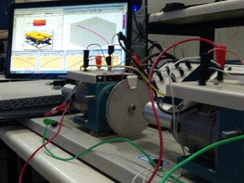
The designed HIL test rig is shown in Fig. 3.

Figure 3.

A schematic of the test rig.

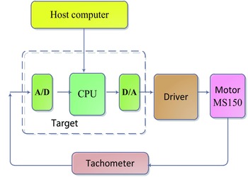
A block diagram of the HIL is shown in Fig. 4. According to Fig. 4, the host computer will do the necessary computations and send the production control signal to the motor driver through the PCI6221 interface board. The propulsion of the motor, as stated in Eq. (10), is based on the speed measured by a tachometer sensor. The tachometer output is converted from analog to digital and then sent to the computer, allowing the computer to generate the required force and torque for driving the ROV’s dynamics.

Figure 4.

A brief view of the hardware-in-the-loop architecture.

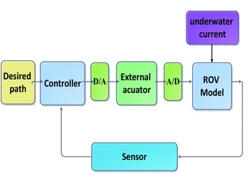
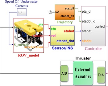
Figure 5 shows the primary control of the ROV model in dynamic Eqs. (1) and (7) in the simulink desktop real-time environment.

Figure 5.

Basic of the proposed closed-loop ROV control.

Some environmental disturbances, such as underwater currents, affect the performance of the ROV. Therefore, this phenomenon is taken into consideration.

5.2. Simulation result

Simulation is performed by executing the test rig as in Fig. 6. Table III shows the parameters of the ROV, while the desired path for the robot is a spiral.

Table III.

The ROV specifications.

Figure 6.

The close-loop ROV control in the MATLAB/SIMULINK environment.

Undesired underwater current velocities $V_{c}=[u_{c}\ \ v_{c}\ \ w_{c}]^{T}$ are defined against the ROV’s motion as in refs. [Reference Hosseini and Seyedtabaii2, Reference García-Valdovinos, Salgado-Jiménez, Bandala-Sánchez, Nava-Balanzar, Hernández-Alvarado and Cruz-Ledesma24]:

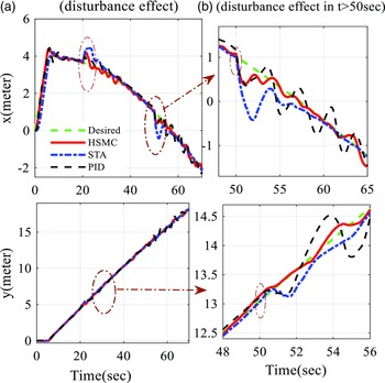
(41) \begin{align} 20\,\textrm{s} & \leq t\lt 50\,\textrm{s}\rightarrow V_{c}=\left[0.5\dfrac{\textrm{m}}{\textrm{s}},0,0\right]^{T}\nonumber\\[3pt] 50\,\textrm{s} & \leq t\lt 100\,\textrm{s}\rightarrow V_{c}=\left[v_{a}\cos \alpha \sin \beta,v_{a}\sin \beta,v_{a}\sin \alpha \cos \beta \right]^{T} \end{align}

where $v_{a}$ is the average current velocity, $\alpha$ is the angle of attack, and $\beta$ is the sideslip angle.

5.2.1. DC motor identification

Primarily, DC servo motors dynamic is identified as ROV thrusters during the SIL simulation, gaining Eq. (42) as the transfer function between motor speed and armature voltage [Reference Adewusi30]:

(42) \begin{equation} G\!\left(s\right)=\frac{\omega \!\left(s\right)}{v_{a}\!\left(s\right)}=\frac{k_{m}}{\left(sJ+B\right)\left(sL_{a}+R_{a}\right)+k_{m}^{2}} \end{equation}

Eq. (42) reduces to a lower order assuming that the armature winding inductance La is insignificant in comparison to the moment of inertia of the motor:

(43) \begin{equation} G\!\left(s\right)=\frac{k_{m}}{Ts+1} \end{equation}

where $T$ and $K_{m}$ , respectively, denote the time and the gain constants of the DC motor. These coefficients are found, according to Fig. 7, in response to a step change as $K_{m}=0.964$ and $T=0.25\,\textrm{s}$ .

Figure 7.

The motor step response.

In Eq. (16), the thrust is a function of the speed propeller. According to the thrust curve of the DC motor in Fig. 8, there exists a dead-zone nonlinearity problem. That means there is no thrust output when the control signal is within the range of [−4, 4.7] volts.

Figure 8.

The thrust curve of DC motor, including a dead zone.

5.2.2. HIL result

The data acquisition card (DAC) Pci6221 has an output voltage bound of $\pm 10$ volts.

However, the software in the loop simulation is performed using the identified parameters of the motor. After that, actual DC motors are employed to replace the thruster model during the HIL test. The tachometer output is sampled at 1 kHz to analyze the frequency spectrum.

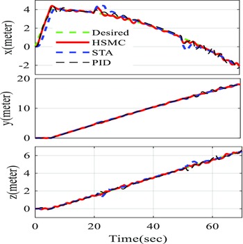
Figure 9 shows the test performed during tracking the desired path in the three directions when using HSMC, STA, and PID controllers in the presence of external disturbance of Eq. (39).

Figure 9.

Displacement in x, y, and z axis using the proposed control procedure.

Figure 10.

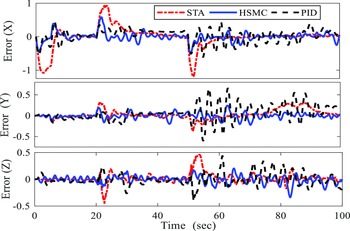
The tracking error in three axis.

Figure 10 shows the tracking error for linear displacement in the three directions obtained from Eq. (44) for HSMC, STA, and PID controllers.

(44) \begin{equation} \text{Error}=(p(i)-p_{\text{command}}(i))\ \ i=1,2,3 \end{equation}

Figure 11 shows the ROV heading during the path following.

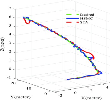
Figure 12 shows a 3D ROV trajectory tracking in 3D during the HIL tests.

Figure 11.

Heading of ROV.

Figure 12.

The test result for 3D position tracking in the HIL rig.

A performance term of integral of the absolute error (IAE) of the tracking task is defined in Eq. (45) ref. [Reference Proaño, Capito, Rosales and Camacho31].

(45) \begin{equation} \overline{\textrm{IAE}}=\frac{\int _{0}^{T}\left| e\!\left(t\right)\right| dt}{T} \end{equation}

where $e(t)$ is the tracking error. Besides and to test which controller has the best performance, the relative error between the two IAE of the controller calculates as in ref. [Reference Proaño, Capito, Rosales and Camacho31]:

(46) \begin{equation} {\Lambda}\!\left(1,2\right)=\frac{\overline{\textrm{IAE}_{1}}-\overline{\textrm{IAE}_{2}}}{\frac{\overline{\textrm{IAE}_{1}}+\overline{\textrm{IAE}_{2}}}{2}}\times 100\% \end{equation}

If ${\Lambda}$ is positive, that means that the performance of controller Eq. (2) is better than Eq. (1) and vice versa for the other controller.

The IAE results in Table IV show that the performance of the HSMC controller is better than other controllers.

The mean square error index of the tracking in the x, y, and z directions is presented in Table V.

Eq. (41) indicates that underwater currents act as an external disturbance to the robot dynamics in the simulation. Figure 13 demonstrates that the HSMC controller performs better than the PID and STA controllers in the presence of this disturbance, delivering a fast and smooth response with minimal overshoot.

Table IV.

IAE indices: square trajectory.

Table V.

The mean square error indices.

Figure 13.

(a) Performance of the controllers against the external disturbance; (b) detailed view of the image (a).

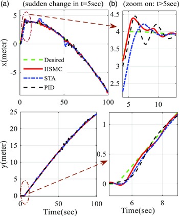
Figure 14 shows that the HSMC controller is more adept at handling sudden changes in ROV motion, offering a fast and smooth response in comparison to the PID and STA controllers.

Figure 14.

(a) Performance of the controllers against the sudden change of direction of the ROV; (b) Detailed view of the image (a).

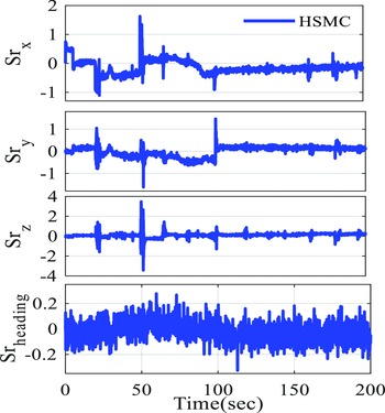
Figure 15 illustrates the proposed HSMC controller, which causes the sliding surfaces to converge in a finite amount of time.

Figure 15.

Sliding surfaces evolve around the origin.

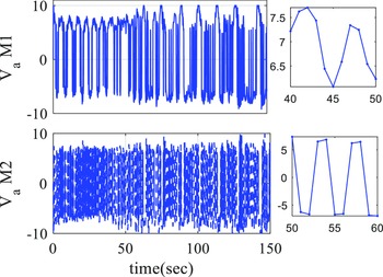
The motor armature voltage is shown in Fig. 16. The voltage bound due to the saturation level of the analog output signal (DAC) of the pci6221 interface board is between [−10, 10] volts. Figure 16 shows the performance of the HSMC controller.

Figure 16.

The armature voltage of T1 and T2.

Figure 17.

The rotation speed of motors 1 and 2.

Figure 18.

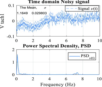
The frequency spectrum and measured speed of motor #1 are shown in the bottom and top, respectively.

As seen in Fig. 16, motors change the direction two to three times every 10 s. These turns are acceptable by the thruster. The frequency of the control signal is about 0.3 Hz, which is satisfactory.

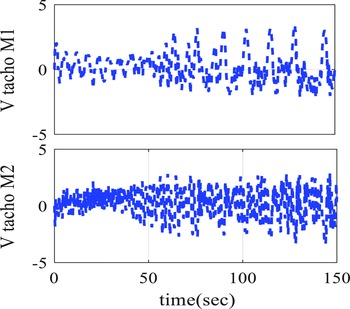
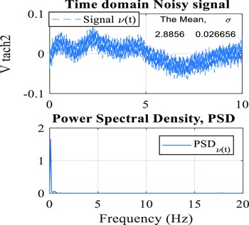
The rotational speeds of motors 1 and 2 as measured by the tachometer are shown in Fig. 17. To further investigate, the speed output’s frequency spectrum is plotted in the time range (10–20) seconds as the speed approaches the steady state, as seen in Figs. 18 and 19.

Figure 19.

The frequency spectrum and measured speed of motor #2 are shown in the bottom and top, respectively.

The spectrum’s frequency reveals that the majority of signals are concentrated around the DC frequency of 0.1 Hz. This indicates that the sampling of each motor’s speed has been done reliably and effectively.