1 Introduction
Barchans are a specific type of sand dunes characterized by their distinct crescentic shape, which includes a windward side, two horns and a slip face on the lee side (Hersen Reference Hersen2005; Parteli, Duran & Herrmann Reference Parteli, Duran and Herrmann2007). They arise on the surfaces of both Earth and Mars as well as in subaqueous environments (Bridges et al.
Reference Bridges, Ayoub, Avouac, Leprince, Lucas and Mattson2012) when the flow is unidirectional and the sand supply on the bedrock is scarce (Andreotti, Claudin & Douady Reference Andreotti, Claudin and Douady2002a
,Reference Andreotti, Claudin and Douady
b
). Their characteristic dimensions scale with the so-called saturation length scale (Hersen, Douady & Andreotti Reference Hersen, Douady and Andreotti2002; Kroy & Guo Reference Kroy and Guo2004)
 $L_{s}=d_{50}(\unicode[STIX]{x1D70C}_{s}/\unicode[STIX]{x1D70C}_{f})$
, where
 $\unicode[STIX]{x1D70C}_{s}$
and
 $\unicode[STIX]{x1D70C}_{f}$
represent the densities of sediment material and fluid respectively and
 $d_{50}$
is the median size of the sediment material, while their spacing has been shown to scale with the thickness of the atmospheric boundary layer or water depth (Andreotti et al.
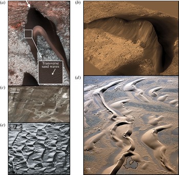
Reference Andreotti, Fourriere, Ould-Kaddour, Murray and Claudin2009). Because of their intriguing shapes and profound impact on aeolian landscapes (see figure 1), barchan dunes have fascinated researchers for several decades (Bagnold Reference Bagnold1941; Howard et al.
Reference Howard, Morton, Gad-El-Hak and Pierce1978; Fisher & Galdies Reference Fisher and Galdies1988). A major challenge in their study, however, arises from the large spatial and temporal scales that aeolian barchans exhibit in nature, which renders the observation of the entire process from their genesis to the long-term evolution impractical if not impossible even with today’s most advanced satellite technology. Most of what we know today about barchans has been derived from photographs and satellite images, laboratory-scale experiments, and relatively simple computational and theoretical models (Werner Reference Werner1999; Andreotti et al.
Reference Andreotti, Claudin and Douady2002a
,Reference Andreotti, Claudin and Douady
b
; Elbelrhiti, Claudin & Andreotti Reference Elbelrhiti, Claudin and Andreotti2005). Available models either omit the coupling of the turbulent flow and the sand transport dynamics completely or take it into account via analytical approaches (Schwammle & Herrmann Reference Schwammle and Herrmann2003; Duran, Parteli & Herrmann Reference Duran, Parteli and Herrmann2010; Genois et al.
Reference Genois, Hersen, du Pont and Grgoire2013; Omidyeganeh & Piomelli Reference Omidyeganeh and Piomelli2013a
,Reference Omidyeganeh and Piomelli
b
; Worman et al.
Reference Worman, Murray, Littlewood, Andreotti and Claudin2013; Parteli et al.
Reference Parteli, Kroy, Tsoar, Andrade and Poschel2014b
).
Naturally occurring barchan dunes: (a) Martian barchan (NASA/JPL-Caltech/University of Arizona) with transverse surface sand waves migrating on the two horns of the barchan shown in the white window; (b) Martian barchan (United States Geographical Survey); (c) aeolian barchans in Peru (Google, DigitalGlobe); (d) aeolian barchans in Namibian desert showing intricate barchan field and transverse dunes where complex bedload transport in the wake of dunes leads to bedrock exposure (dashed line) (Google, DigitalGlobe); (e) experimentally observed subaqueous barchans of Mantz (Reference Mantz1978) in which flow is from left to right.

Almost all of the existing models are based on the landmark work of Sauermann, Kroy & Herrmann (Reference Sauermann, Kroy and Herrmann2001) and Kroy, Sauermann & Herrmann (Reference Kroy, Sauermann and Herrmann2002a
,Reference Kroy, Sauermann and Herrmann
b
), who introduced a mathematical ‘minimum model’ to reproduce the formation and development of aeolian barchan fields. The minimum models are based on the following three fundamental assumptions: (i) the bed shear stress exerted on the mobile bed can be prescribed via stationary wind fields, the so-called ‘wind strength’ (Parteli et al.
Reference Parteli, Kroy, Tsoar, Andrade and Poschel2014b
); (ii) the turbulent flow around the smooth terrain of a barchan dune is perfectly symmetric, and thus the flow over the upwind side and wake of the dune can be phenomenologically parametrized via analytical approaches (Kroy et al.
Reference Kroy, Sauermann and Herrmann2002a
; Schwammle & Herrmann Reference Schwammle and Herrmann2003); (iii) the feedback effect of sand particles on the turbulent flow can be taken into consideration by incorporating the saturation length
 $L_{s}$
in the calculation of the unidirectional sediment flux (Sauermann et al.
Reference Sauermann, Rognon, Poliakov and Herrmann2000, Reference Sauermann, Kroy and Herrmann2001; Kroy & Guo Reference Kroy and Guo2004; Bridges et al.
Reference Bridges, Ayoub, Avouac, Leprince, Lucas and Mattson2012; Zhang et al.
Reference Zhang, Narteau, Rozier and du Pont2012; Parteli et al.
Reference Parteli, Kroy, Tsoar, Andrade and Poschel2014b
).
Numerical approaches for barchan dune simulation based on the minimum models include (i) the skeleton model (Guignier et al. Reference Guignier, Niyah, Nishimori, Lague and Valance2013), which is mainly implemented to analytically calculate the lateral sediment flux to render the minimum model capable of computing sediment fluxes in streamwise and spanwise directions, (ii) the cellular automaton model (Werner Reference Werner1995), in which the sediment flux is calculated via a set of probabilistic rules, and (iii) the dune-field models (Lima et al. Reference Lima, Sauermann, Herrmann and Kroy2002; Parteli & Herrmann Reference Parteli and Herrmann2003; Kok et al. Reference Kok, Parteli, Michaels and Karam2012), in which the individual barchan dunes are treated as ‘interacting particles’ (Parteli et al. Reference Parteli, Kroy, Tsoar, Andrade and Poschel2014b ) with identical height that interact with one another by interdune sand flux that is a function of the distance between the two neighbouring dunes. In spite of small differences in their formulation, there are two unifying themes among all such minimum model-based approaches: (1) they do not consider the spatial and temporal complexity of the turbulent flow that drives the emergence and evolution of the dune fields and (2) they do not account for the coupled interaction between the flow and the evolving bed geometry (Parteli & Herrmann Reference Parteli and Herrmann2003). These simplifications notwithstanding, however, existing minimal models have been able to reproduce many of the underlying features of barchan evolution. For example, such models have been able to reproduce and underscore the importance of phenomena such as barchan migration, merging and calving (the birth of new small barchans from the horns of large barchans) in the formation of quasiequilibrium barchan fields (Sauermann et al. Reference Sauermann, Rognon, Poliakov and Herrmann2000, Reference Sauermann, Kroy and Herrmann2001, Reference Sauermann, Andrade, Maiac, Costab, Araujod and Herrmanna2003; Andreotti Reference Andreotti2004; Kroy & Guo Reference Kroy and Guo2004; Elbelrhiti et al. Reference Elbelrhiti, Claudin and Andreotti2005; Bridges et al. Reference Bridges, Ayoub, Avouac, Leprince, Lucas and Mattson2012; Zhang et al. Reference Zhang, Narteau, Rozier and du Pont2012; Khosronejad & Sotiropoulos Reference Khosronejad and Sotiropoulos2014; Parteli et al. Reference Parteli, Duran, Bourke, Tsoar, Pschel and Herrmann2014a ,Reference Parteli, Kroy, Tsoar, Andrade and Poschel b ). A common limitation of these models, however, is their tendency to produce smooth barchan shapes and, thus, their inherent inability to capture the complex transverse surface waves observed in nature along the windward side of large aeolian barchans (Sauermann et al. Reference Sauermann, Andrade, Maiac, Costab, Araujod and Herrmanna2003; Andreotti Reference Andreotti2004; Parteli et al. Reference Parteli, Duran, Bourke, Tsoar, Pschel and Herrmann2014a ).
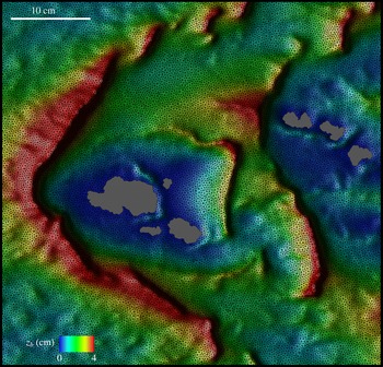
To clarify the nature of these so-called transverse surface waves, we note that, in general, transverse sand waves form when there is adequate sediment supply and the local near-bed turbulent flow conditions are suitable to destabilize the bedload layer and ultimately lead to a self-organized state with transverse-to-the-flow quasiequilibrium dunes spanning the entire flow domain (Fisher & Galdies Reference Fisher and Galdies1988; Hersen Reference Hersen2005) – for a detailed description of the process see Khosronejad & Sotiropoulos (Reference Khosronejad and Sotiropoulos2014). One of the main conditions that is necessary for the formation of barchan dunes, however, is the scarcity of the sediment supply over bedrock. When large barchans have emerged, conditions supporting the formation of transverse waves may emerge locally on the windward side of barchans where sediment has accumulated and the turbulent flow accelerates as it is directed towards the horns of the barchans. Therefore, along the windward side of a large barchan, increments of bed shear stress may arise that are sufficiently large to destabilize the surface of the barchans and lead to the formation of sand waves that are transverse to the local flow direction and migrate towards the barchan horns. Such transverse surface sand waves have indeed been observed in nature, as highlighted in figure 1(a).
Elbelrhiti et al. (Reference Elbelrhiti, Claudin and Andreotti2005) argued that such transverse surface sand waves are fundamentally important as they provide the mechanism for sand loss that prevents dune fields from merging into a single giant dune, and thus control dune patterns and sizes. To the best of our knowledge, this important feature of barchan dune morphology has yet to be captured numerically. It is the key hypothesis of our work that this state of affairs should be attributed to the lack of computational models of barchan dunes.
To probe the validity of this hypothesis, we employ herein a recently developed high-fidelity large-eddy simulation (LES) computational model that couples turbulent flow with sand-bed morphodynamics (Khosronejad & Sotiropoulos Reference Khosronejad and Sotiropoulos2014; Sotiropoulos & Khosronejad Reference Sotiropoulos and Khosronejad2016) to present a complete description of the entire process of barchan dune genesis and long-term evolution in a subaqueous environment: a turbulent flow through a straight rectangular open channel with a rigid bed (the bedrock) covered initially by a finite amount of uniformly distributed non-cohesive sediment. The simulation starts from the initially flat sand bed and proceeds for several hours of physical time until a quasiequilibrium barchan field emerges. We select subaqueous barchans because their dynamics is similar to aeolian dunes (Andreotti et al. Reference Andreotti, Fourriere, Ould-Kaddour, Murray and Claudin2009), but their spatial and temporal scales are several orders of magnitude smaller, thus making the numerical simulation of the complete process computationally tractable (Franklin & Charru Reference Franklin and Charru2011; Charru & Franklin Reference Charru and Franklin2012). Our results show conclusively that a model that couples the turbulent flow with the bed morphodynamics at sufficiently fine numerical resolution is able to simulate the entire process of genesis and long-term evolution of barchan fields as observed in nature. More specifically, our model is able to capture the onset of transverse sand waves on the surface of the dunes and conclusively illustrate their role in establishing barchan fields at quasiequilibrium. It is important to note that we report herein the results of high-fidelity simulations in the sense that the spatial and temporal resolution of the coupled hydro–morphodynamic LES model is sufficiently fine to resolve not only the structure and dynamics of large quasiequilibrium barchans but also the much smaller size transverse sand waves that arise on the windward side of the barchans. To the best of knowledge, simulations of resolution able to capture the profound effect these transverse waves have on sustaining equilibrium barchan fields have not been previously reported in the literature. In this sense, the LES is used herein as a tool of scientific discovery, enabling us to conduct numerical experiments of sufficient detail and physical realism to reproduce and explain the governing mechanisms of a range of complex geophysical phenomena that have been observed in nature. We also note that the LES does not resolve the near-bed viscous sublayer; rather, a wall model approach is incorporated in our simulations. In our previous work (Khosronejad & Sotiropoulos Reference Khosronejad and Sotiropoulos2014), however, we have conclusively shown through systematic grid refinement studies that a wall model on a grid with near-bed grid spacing of approximately 20 wall units is sufficiently fine to accurately simulate the onset and evolution of transverse dunes.
The main focus of this paper is on the morphodynamic aspects of barchan dunes, and consequently the dynamics of the turbulent flow that drives the emergence of barchan fields is only briefly discussed herein. In Part II of this work, currently in preparation, we will focus on the details of the turbulent flow over the bed of evolving barchans during various stages of their development.
This paper is organized as follows. In § 2, we present a brief description of the governing equations and numerical methods we used to develop our coupled hydro–morphodynamics model. In § 3, we describe the test case we use to simulate subaqueous barchan field. In § 4, we present the simulated results, from the initiation of bed deformation to the development of equilibrium barchan fields. Finally, in § 5, we discuss our findings relative to previous work in the field and summarize the new insights derived from our simulations. A quantitative validation of our method for a case previously studied experimentally and computationally (Apsley & Stansby Reference Apsley and Stansby2008) involving the evolution of a single Gaussian dune in a turbulent open channel flow is reported in appendix A.
2 The coupled hydro–morphodynamic model
We employ a novel fully coupled hydro–morphodynamics model, the so-called Virtual Flow Simulator (VFS-Rivers) developed by Sotiropoulos and co-workers at the St. Anthony Falls Laboratory, University of Minnesota. The code solves numerically the spatially filtered continuity and Navier–Stokes equations with the Boussinesq assumption to simulate incompressible stratified turbulent flow of dilute water–sediment mixture over evolving mobile sediment beds with arbitrarily complex morphology. To simulate the coupling between the hydro- and morphodynamics, we employ a partitioned fluid–structure interaction (FSI) approach (Borazjani, Ge & Sotiropoulos Reference Borazjani, Ge and Sotiropoulos2008; Khosronejad et al. Reference Khosronejad, Kang, Borazjani and Sotiropoulos2011), by which the problem is partitioned into the fluid and sediment domains, and solve the governing equations for the stratified flow and the bed morphodynamics separately in each domain, accounting for the interaction of the two domains by applying boundary conditions at the fluid/sediment interface. The dynamically evolving shape of the bed is determined by solving the Exner–Polya equation in a coupled manner with the flow and suspended sediment equations (see §§ 2.1 and 2.2). The code is parallelized using the message passing interface (MPI) communication standard and runs on parallel high-performance supercomputers. The governing equations and numerical methods implemented in the VFS-Rivers code have been extensively described in a series of papers from our group (see, e.g., Khosronejad et al. Reference Khosronejad, Hill, Kang and Sotiropoulos2013; Khosronejad, Kozarek & Sotiropoulos Reference Khosronejad, Kozarek and Sotiropoulos2014; Khosronejad & Sotiropoulos Reference Khosronejad and Sotiropoulos2014; Khosronejad et al. Reference Khosronejad, Kozarek, Palmsten and Sotiropoulos2015) – the same papers report extensive validation of various aspects of VFS-Rivrs for a broad range of test cases. Here, we only provide a brief description of the model for the sake of completeness of this paper. In appendix A, we also report yet another quantitative validation of the model for a test case involving the interaction of an initially symmetric mound of sediment (a Gaussian hill) in a turbulent open channel flow (Apsley & Stansby Reference Apsley and Stansby2008).
2.1 Resolved flow and sediment concentration field
The governing equations for the flow field and suspended sediment concentration (in volume fraction),
 $\unicode[STIX]{x1D713}$
, read in compact tensor notation (repeated indices, i.e.
 $j$
,
 $k$
and
 $l$
, imply summation over 1–3) and curvilinear coordinates
 $\{\unicode[STIX]{x1D709}^{i}\}$
as follows (
 $i=1,2$
or 3):
 $$\begin{eqnarray}\displaystyle \displaystyle J\frac{\unicode[STIX]{x2202}U^{j}}{\unicode[STIX]{x2202}\unicode[STIX]{x1D709}^{j}}=0, & & \displaystyle\end{eqnarray}$$
 $$\begin{eqnarray}\displaystyle \displaystyle \frac{1}{J}\frac{\unicode[STIX]{x2202}U^{i}}{\unicode[STIX]{x2202}t} & = & \displaystyle \frac{\unicode[STIX]{x1D709}_{l}^{i}}{J}\left(-\frac{\unicode[STIX]{x2202}}{\unicode[STIX]{x2202}\unicode[STIX]{x1D709}^{j}}(U^{j}u_{l})+\frac{1}{\unicode[STIX]{x1D70C}_{f}}\frac{\unicode[STIX]{x2202}}{\unicode[STIX]{x2202}\unicode[STIX]{x1D709}^{j}}\left(\unicode[STIX]{x1D707}\frac{\unicode[STIX]{x1D60E}^{jk}}{J}\frac{\unicode[STIX]{x2202}u_{l}}{\unicode[STIX]{x2202}\unicode[STIX]{x1D709}^{k}}\right)\right.\nonumber\\ \displaystyle & & \displaystyle \left.-\,\frac{1}{\unicode[STIX]{x1D70C}_{f}}\frac{\unicode[STIX]{x2202}}{\unicode[STIX]{x2202}\unicode[STIX]{x1D709}^{j}}\left(\frac{\unicode[STIX]{x1D709}_{l}^{j}p}{J}\right)-\frac{1}{\unicode[STIX]{x1D70C}_{f}}\frac{\unicode[STIX]{x2202}\unicode[STIX]{x1D70F}_{lj}}{\unicode[STIX]{x2202}\unicode[STIX]{x1D709}^{j}}+\frac{\overline{\unicode[STIX]{x1D70C}}-\unicode[STIX]{x1D70C}_{f}}{\unicode[STIX]{x1D70C}_{f}}g\left(\frac{\unicode[STIX]{x1D6FF}_{i3}}{J}\right)\right),\end{eqnarray}$$
 $$\begin{eqnarray}\displaystyle \displaystyle \frac{1}{J}\frac{\unicode[STIX]{x2202}(\unicode[STIX]{x1D70C}_{f}\unicode[STIX]{x1D713})}{\unicode[STIX]{x2202}t}+\frac{\unicode[STIX]{x2202}}{\unicode[STIX]{x2202}\unicode[STIX]{x1D709}^{j}}(\unicode[STIX]{x1D70C}_{f}\unicode[STIX]{x1D713}(U^{j}-W^{j}\unicode[STIX]{x1D6FF}_{i3}))=\frac{\unicode[STIX]{x2202}}{\unicode[STIX]{x2202}\unicode[STIX]{x1D709}^{j}}\left((\unicode[STIX]{x1D707}+\unicode[STIX]{x1D70E}^{\ast }\unicode[STIX]{x1D707}_{t})\frac{\unicode[STIX]{x1D60E}^{jk}}{J}\frac{\unicode[STIX]{x2202}\unicode[STIX]{x1D713}}{\unicode[STIX]{x2202}\unicode[STIX]{x1D709}^{k}}\right)\!. & & \displaystyle\end{eqnarray}$$
Here,
 $J$
is the Jacobian of the geometric transformation given by
 $J=|\unicode[STIX]{x2202}(\unicode[STIX]{x1D709}^{1},\unicode[STIX]{x1D709}^{2},\unicode[STIX]{x1D709}^{3})/\unicode[STIX]{x2202}(x_{1},x_{2},x_{3})|$
;
 $x_{1}$
,
 $x_{2}$
and
 $x_{3}$
are the streamwise, spanwise and vertical coordinates respectively;
 $\unicode[STIX]{x1D709}_{l}^{i}=\unicode[STIX]{x2202}\unicode[STIX]{x1D709}^{i}/\unicode[STIX]{x2202}x_{l}$
are the transformation metrics;
 $u_{i}$
is the
 $i$
th Cartesian velocity component;
 $U^{i}=(\unicode[STIX]{x1D709}_{m}^{i}/J)u_{m}$
is the contravariant volume flux;
 $\unicode[STIX]{x1D60E}^{jk}=\unicode[STIX]{x1D709}_{l}^{j}\unicode[STIX]{x1D709}_{l}^{k}$
are the components of the contravariant metric tensor;
 $p$
is the pressure;
 $\unicode[STIX]{x1D70F}_{lj}$
is the subgrid stress tensor for the LES model, which in this work is obtained using the dynamic Smagorinsky model (Smagorinsky Reference Smagorinsky1963; Germano et al.
Reference Germano, Piomelli, Moin and Cabot1991; Kang & Sotiropoulos Reference Kang and Sotiropoulos2011);
 $g$
is the gravitational acceleration;
 $\unicode[STIX]{x1D6FF}$
is the Kronecker delta;
 $\overline{\unicode[STIX]{x1D70C}}$
is the density of sediment–water mixture (
 $=\unicode[STIX]{x1D70C}_{f}(1-\unicode[STIX]{x1D713})+\unicode[STIX]{x1D70C}_{s}\unicode[STIX]{x1D713}$
);
 $W^{j}$
is the contravariant volume flux of suspended sediment (
 $=(\unicode[STIX]{x1D709}_{3}^{j}/J)w_{s}$
);
 $\unicode[STIX]{x1D70E}^{\ast }$
is the Schmidt number (
 $=$
0.75) (Khosronejad et al.
Reference Khosronejad, Salehi, Rennie and Gholami2008);
 $\unicode[STIX]{x1D707}$
is the dynamic viscosity of fluid;
 $\unicode[STIX]{x1D707}_{t}$
is the eddy viscosity, which is obtained using the dynamic Smagorinsky model (see, for details, Khosronejad & Sotiropoulos Reference Khosronejad and Sotiropoulos2014);
 $w_{s}$
is the settling velocity of sediment particles.
The suspended sediment concentration is assumed to have negligible effect on the momentum of fluid flow. This is a common assumption in Eulerian coupled flow–morphodynamics models for cases in which the suspended sediment concentration is small (
 ${\leqslant}0.01$
) (Zedler & Street Reference Zedler and Street2006; Chou & Fringer Reference Chou and Fringer2010; Khosronejad et al.
Reference Khosronejad, Hansen, Kozarek, Guentzel, Hondzo, Guala, Wilcock, Finlay and Sotiropoulos2016), as is the case in this work. We do, however, take into account the impact of the stratification and bulk of suspended sediment material on the resolved flow field using the Boussinesq term in the momentum equation – see the last term on the right-hand side of (2.2). Finally, the governing equations for flow and sediment concentration fields are discretized on a hybrid staggered/non-staggered grid using second-order-accurate finite-difference formulae and integrated in time with an efficient fractional-step method. For a detailed description of the numerical methods we used to discretize (2.1)–(2.3), the reader is referred to Kang et al. (Reference Kang, Lightbody, Hill and Sotiropoulos2011), Kang, Khosronejad & Sotiropoulos (Reference Kang, Khosronejad and Sotiropoulos2012), Khosronejad & Sotiropoulos (Reference Khosronejad and Sotiropoulos2014) and Sotiropoulos & Khosronejad (Reference Sotiropoulos and Khosronejad2016).
2.2 Morphodynamics
We employ the Exner–Polya, the sediment material mass balance, equation to simulate the evolution of bed elevation,
 $z_{b}$
, as follows (Paola & Voller Reference Paola and Voller2005):
 $$\begin{eqnarray}\displaystyle & \displaystyle (1-\unicode[STIX]{x1D6FE})\frac{\unicode[STIX]{x2202}z_{b}}{\unicode[STIX]{x2202}t}+\unicode[STIX]{x1D735}_{H}\boldsymbol{\cdot }\unicode[STIX]{x1D731}+\unicode[STIX]{x1D6FA}_{E}-\unicode[STIX]{x1D6FA}_{D}=0, & \displaystyle\end{eqnarray}$$
 $$\begin{eqnarray}\displaystyle & \displaystyle \unicode[STIX]{x1D735}_{H}=\left[\frac{\unicode[STIX]{x2202}}{\unicode[STIX]{x2202}x},\frac{\unicode[STIX]{x2202}}{\unicode[STIX]{x2202}y},0\right], & \displaystyle\end{eqnarray}$$
 $$\begin{eqnarray}\displaystyle & \displaystyle \unicode[STIX]{x1D731}(x,y)=\unicode[STIX]{x1D6E9}_{b}\int _{\unicode[STIX]{x1D702}_{b}}^{\unicode[STIX]{x1D702}_{b}+\Vert \unicode[STIX]{x1D739}_{\boldsymbol{b}}\Vert }\boldsymbol{u}_{b}\,\text{d}\unicode[STIX]{x1D702}. & \displaystyle\end{eqnarray}$$
Here,
 $\unicode[STIX]{x1D6FE}$
is the sediment material porosity;
 $\unicode[STIX]{x1D731}$
is the bedload flux vector;
 $\unicode[STIX]{x1D739}_{\boldsymbol{b}}$
is the vertical vector along the
 $z$
-axis with a length equal to the bedload layer thickness (
 $\Vert \unicode[STIX]{x1D739}_{\boldsymbol{b}}\Vert$
), which is assumed to be equal to
 $2d_{50}$
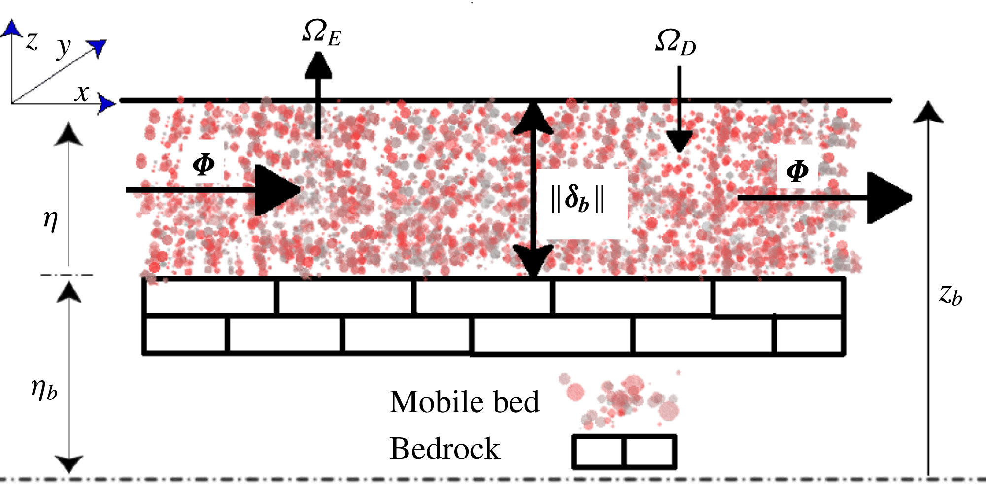
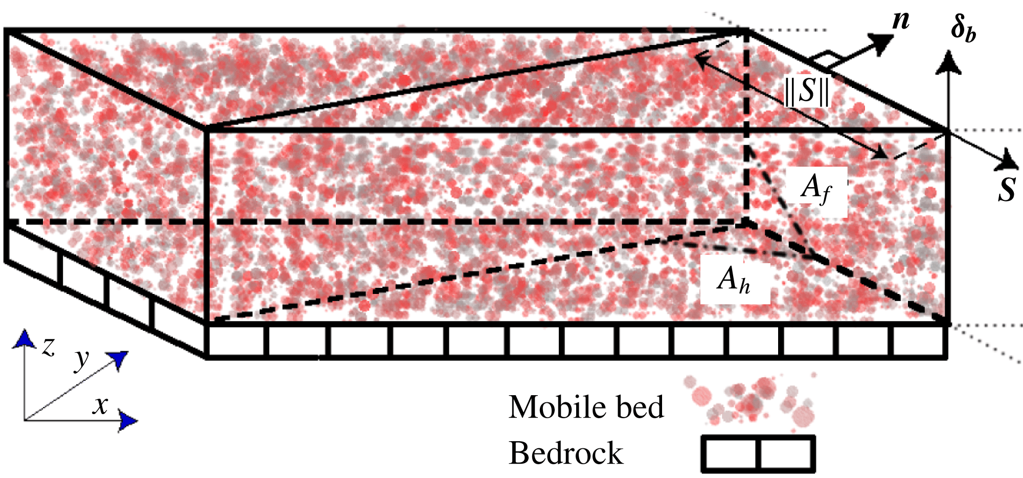
(see figures 2 and 3);
 $\boldsymbol{u}_{b}=(u_{b},v_{b},w_{b})$
is the velocity vector of sediment particles within the bedload layer and is calculated as we discuss below;
 $\unicode[STIX]{x1D6FA}_{E}$
is the rate of entrainment of bed material into suspension;
 $\unicode[STIX]{x1D6FA}_{D}$
is the rate at which suspended load is deposited on the mobile bed;
 $\unicode[STIX]{x1D6E9}_{b}$
is the average bedload concentration within the bedload layer. As in other numerical studies (see, e.g., Olsen & Kjellesvig Reference Olsen and Kjellesvig1998; Roulund et al.
Reference Roulund, Sumer, Fredsoe and Michelsen2005; Chou & Fringer Reference Chou and Fringer2010; Nabi et al.
Reference Nabi, de Vriend, Mosselman, Sloff and Shimizu2012), we employ a mean-flow-based equation to calculate the average bedload concentration as a function of mean-flow characteristics and the Galileo number (
 $G_{a}$
), which is a measure of the ratio between gravitational and viscous forces acting on a sediment particle and can be written in the form of a Reynolds-number-like parameter (van Rijn Reference van Rijn1993; Uhlmann & Doychev Reference Uhlmann and Doychev2014; Sotiropoulos & Khosronejad Reference Sotiropoulos and Khosronejad2016),
 $$\begin{eqnarray}\displaystyle & \displaystyle \unicode[STIX]{x1D6E9}_{b}=f\left(G_{a},T,\frac{D}{\Vert \unicode[STIX]{x1D739}_{\boldsymbol{b}}\Vert }\right), & \displaystyle\end{eqnarray}$$
 $$\begin{eqnarray}\displaystyle & \displaystyle G_{a}=\frac{\unicode[STIX]{x1D70C}_{f}u_{g}d_{50}}{\unicode[STIX]{x1D707}}, & \displaystyle\end{eqnarray}$$
 $$\begin{eqnarray}\displaystyle & \displaystyle u_{g}=\sqrt{gd_{50}\frac{\unicode[STIX]{x1D70C}_{s}-\unicode[STIX]{x1D70C}_{f}}{\unicode[STIX]{x1D70C}_{f}}}, & \displaystyle\end{eqnarray}$$
 $$\begin{eqnarray}\displaystyle & \displaystyle T=\frac{\unicode[STIX]{x1D70F}_{0}}{\unicode[STIX]{x1D70F}_{cr}}-1, & \displaystyle\end{eqnarray}$$
where
 $u_{g}$
is a measure of the settling velocity of the sediment particles,
 $T$
is the effective bed shear stress,
 $\unicode[STIX]{x1D70F}_{0}$
is the bed shear stress and
 $\unicode[STIX]{x1D70F}_{cr}$
is the critical bed shear stress, which is a function of
 $G_{a}$
. Among the most commonly used mean-flow-based equations for the bedload concentrations (Fredsoe Reference Fredsoe1974; Engelund & Fredsoe Reference Engelund and Fredsoe1976, Reference Engelund and Fredsoe1982; van Rijn Reference van Rijn1993), we employed herein the van Rijn pickup function (van Rijn Reference van Rijn1984).
Schematic of mobile-bed characteristics in the vertical direction (Sotiropoulos & Khosronejad Reference Sotiropoulos and Khosronejad2016).

The underlying assumption in our morphodynamics model is that the sediment particle velocity in the bedload layer depends on the flow field at the edge of the bedload layer. Therefore, we do not solve for the particle momentum equation; instead, the sediment particle velocity (
 $\boldsymbol{u}_{b}$
) is obtained by near-bed interpolation and as a function of the near-bed flow velocity (
 $\boldsymbol{u}_{f}$
), shear velocity (
 $u_{\ast }$
) and the thickness of the bedload layer (Olsen & Kjellesvig Reference Olsen and Kjellesvig1998; Roulund et al.
Reference Roulund, Sumer, Fredsoe and Michelsen2005; Zedler & Street Reference Zedler and Street2006; Khosronejad et al.
Reference Khosronejad, Rennie, Salehi and Townsend2007; Duc & Rodi Reference Duc and Rodi2008; Khosronejad et al.
Reference Khosronejad, Kang, Borazjani and Sotiropoulos2011; Khosronejad, Kang & Sotiropoulos Reference Khosronejad, Kang and Sotiropoulos2012; Khosronejad et al.
Reference Khosronejad, Hill, Kang and Sotiropoulos2013, Reference Khosronejad, Kozarek and Sotiropoulos2014, Reference Khosronejad, Kozarek, Palmsten and Sotiropoulos2015). In order to find the near-bed flow velocity, we reconstruct the flow velocity at the edge of the bedload layer using a wall model that is explained in detail in Khosronejad & Sotiropoulos (Reference Khosronejad and Sotiropoulos2014).
Once
 $\boldsymbol{u}_{b}$
and
 $\unicode[STIX]{x1D6E9}_{b}$
(from (2.7)) are known, they are plugged in (2.6) to obtain
 $\unicode[STIX]{x1D731}$
and solve the Exner–Polya equation. In the context of the curvilinear immersed boundary (CURVIB) method (see § 2.4 below), we discretize the fluid/sediment interface with an unstructured triangular grid (figure 3) and solve the Exner–Polya equation on the unstructured mesh using a finite volume method. Using the divergence theorem, (2.4) can be discretized at a given bed-surface triangular element as follows (Khosronejad & Sotiropoulos Reference Khosronejad and Sotiropoulos2014):
 $$\begin{eqnarray}(1-\unicode[STIX]{x1D6FE})\frac{\unicode[STIX]{x0394}z_{b}}{\unicode[STIX]{x0394}t}+\frac{1}{A_{h}}\mathop{\sum }_{ie}[\unicode[STIX]{x1D731}\boldsymbol{\cdot }\langle \boldsymbol{S}\times \unicode[STIX]{x1D739}_{\boldsymbol{b}}\rangle ]_{i_{e}}=\unicode[STIX]{x1D6FA}_{D}-\unicode[STIX]{x1D6FA}_{E},\end{eqnarray}$$
where the summation is carried out over the three edges of the triangular element (
 $i_{e}=1,2,3$
),
 $\unicode[STIX]{x0394}z_{b}$
is the bed elevation change over time step
 $\unicode[STIX]{x0394}t$
,
 $A_{h}$
is the horizontal projected area of the triangular cell face and
 $\boldsymbol{S}$
is the vector along a cell edge with a length equal to the edge length (
 $\Vert \boldsymbol{S}\Vert$
) (see figure 3).
Schematic of a mobile bed element in the bedload layer and definition of the normal vector (
 $\boldsymbol{n}=\boldsymbol{S}\times \unicode[STIX]{x1D739}_{\boldsymbol{b}}$
), side-face area (
 $A_{f}$
) and horizontal projected area (
 $A_{h}$
) of a bed cell (Sotiropoulos & Khosronejad Reference Sotiropoulos and Khosronejad2016).

2.3 Sand-slide algorithm
In our approach, during each time step of the numerical algorithm, we examine and correct the calculated bed surface slopes at the end of each hydro–morphodynamics time step to avoid non-physical slopes for the fluid/sediment interface. The calculated surface slope is not allowed to be greater than that of the angle of repose of sediment material,
 $\unicode[STIX]{x1D711}$
. To do so, we use a mass-conservative sand-slide module, which finds the non-physical local slopes and redistributes the sediment mass among neighbouring bed cells so that no local bed surface slope exceeds the angle of repose.
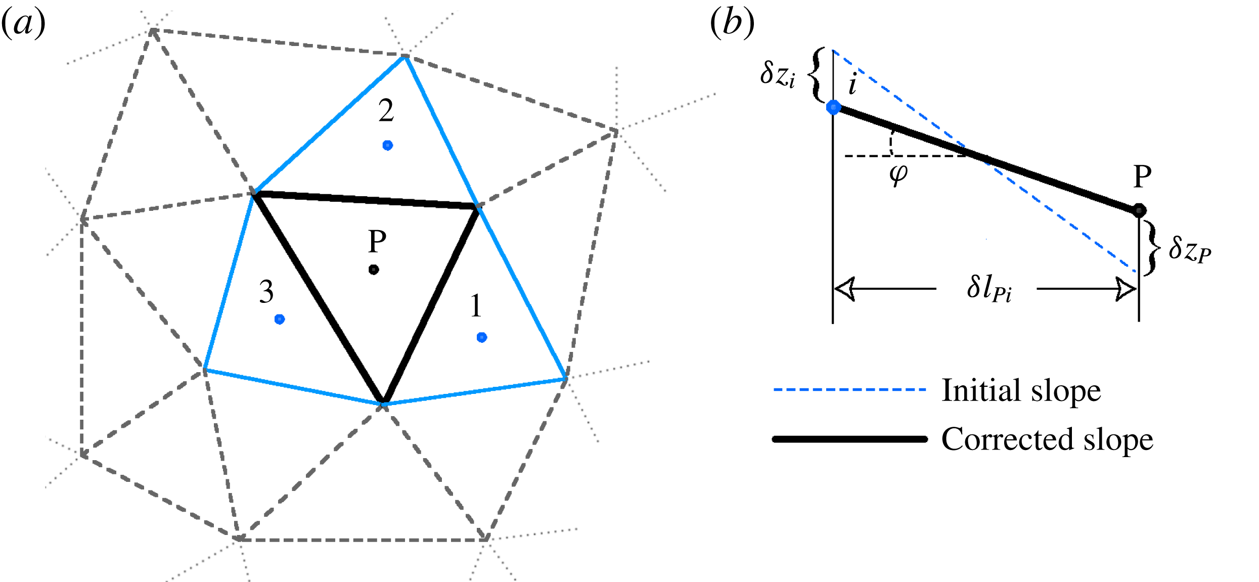
Our sand-slide model is described as follows with reference to figure 4. If the angle between the centre point ‘P’ and any one of the three adjacent cell centres ‘
 $i$
’ (in figure 4) exceeds
 $\unicode[STIX]{x1D711}$
, sediment material is redistributed among neighbouring cells to form a new slope equal to the angle of repose (figure 4
b). This is implemented by applying corrections
 $\unicode[STIX]{x1D6FF}z_{P}$
and
 $\unicode[STIX]{x1D6FF}z_{i}$
to the bed elevations obtained from the mass balance (2.11) at point ‘P’ (
 $z_{P}$
) and its
 $i$
th neighbour (
 $z_{i}$
) respectively for which the bed slope between the two cells whose centroids are
 $\unicode[STIX]{x1D6FF}l_{Pi}$
apart exceeds the material angle of repose using the following equation (Khosronejad et al.
Reference Khosronejad, Kang, Borazjani and Sotiropoulos2011):
 $$\begin{eqnarray}\frac{\langle z_{P}+\unicode[STIX]{x1D6FF}z_{P}\rangle -\langle z_{i}+\unicode[STIX]{x1D6FF}z_{i}\rangle }{\unicode[STIX]{x1D6FF}l_{Pi}}=\tan \unicode[STIX]{x1D711}.\end{eqnarray}$$
Schematics of symbols used in the sand-slide algorithm with an unstructured triangular bed mesh system. The black and blue solid lines in (a) show the central bed cell ‘P’ and its neighbouring cells (
 $i=1,2,3$
) respectively. The blue dashed and black solid lines in (b) show the initial and corrected slopes between cell centres of cell ‘P’ and its neighbouring cells respectively (Khosronejad et al.
Reference Khosronejad, Kang, Borazjani and Sotiropoulos2011; Sotiropoulos & Khosronejad Reference Sotiropoulos and Khosronejad2016).

The elevation corrections are computed by balancing the sediment mass among cell ‘P’ and its three adjacent cells (whose horizontal projected areas are equal to
 $A_{hP}$
and
 $A_{hi}$
respectively) as follows Khosronejad et al. (Reference Khosronejad, Kang, Borazjani and Sotiropoulos2011):
 $$\begin{eqnarray}A_{hP}\unicode[STIX]{x1D6FF}z_{P}=\mathop{\sum }_{i=1,2,3}A_{hi}\unicode[STIX]{x1D6FF}z_{i}.\end{eqnarray}$$
Once the Exner–Polya equation (2.11) is solved, the entire bed is swept to identify elements whose maximum surface slope is larger than the angle of repose. The sand-slide algorithm is then applied only to those identified elements. Since a single sweep is not sufficient to identify and correct all element surfaces whose surface slope exceeds the angle of repose, we apply the above algorithm iteratively until all surface slopes are smaller than the material angle of repose. The iterative process is declared converged when the bed cell steepest surface angle is less than or equal to 0.99 of the angle of repose of the bed material. To eliminate bias in the final solution, the iterative algorithm is implemented through successive sweeps of alternating direction. Usually, 2–4 iterations are enough for the sand-slide algorithm to converge (for more details, see Khosronejad et al. (Reference Khosronejad, Kang, Borazjani and Sotiropoulos2011) and Sotiropoulos & Khosronejad (Reference Sotiropoulos and Khosronejad2016)).
2.4 The curvilinear immersed boundary method
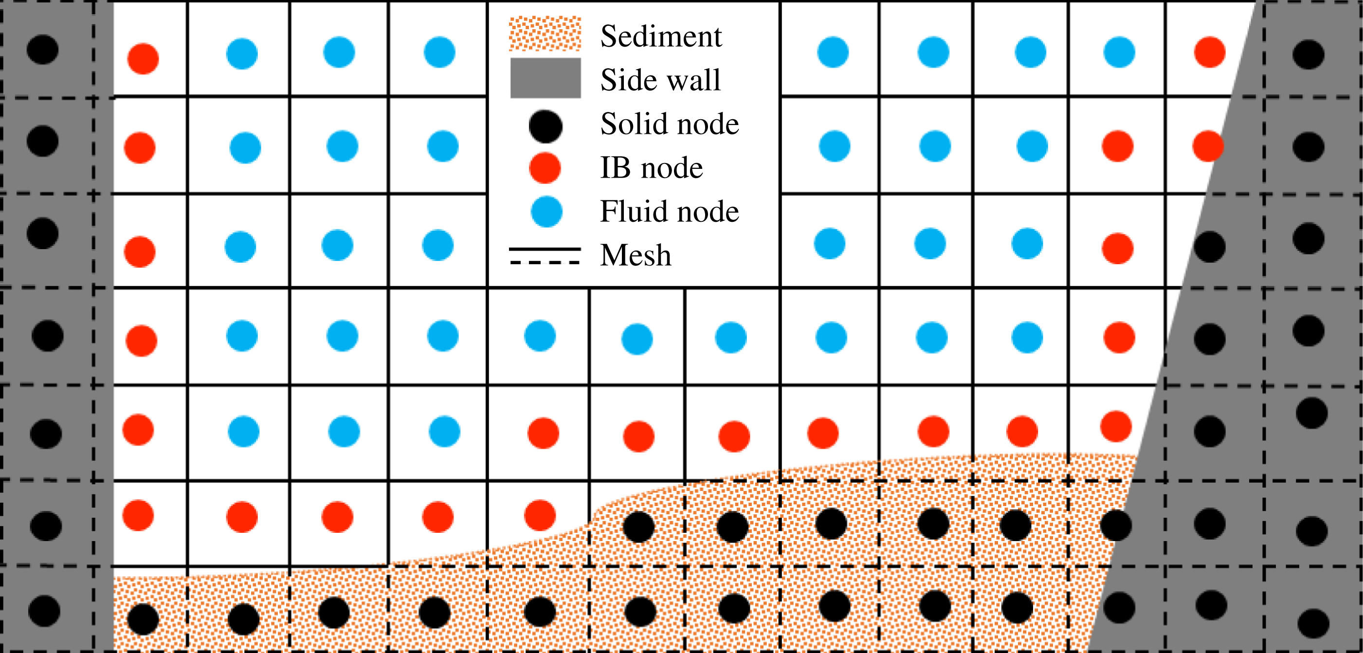
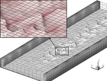
The arbitrarily complex sand-bed geometry that emerges when barchan fields arise and begin to grow and migrate is handled using the sharp-interface CURVIB method of Ge & Sotiropoulos (Reference Ge and Sotiropoulos2007). The background computational domain we consider herein is a straight open channel (see figure 6). We employ a background grid that outlines the actual channel geometry and is sufficiently deep to contain the fluid/sediment interface at all times. In this case, a Cartesian mesh is used as background grid (Khosronejad & Sotiropoulos Reference Khosronejad and Sotiropoulos2014). The fluid/sediment interface is discretized with an unstructured triangular grid and treated as a sharp-interface immersed boundary in accordance with the CURVIB formulation. The governing equations are solved at the background grid nodes in the fluid phase (fluid nodes) with boundary conditions specified at fluid nodes in the immediate vicinity of the fluid/sediment interfaces (denoted as immersed boundary (IB) nodes) (see figure 5 for a schematic description). The nodes inside the solid walls and the sediment layer at the channel bottom are blanked out from the simulation. Boundary conditions for the velocity field are reconstructed at all IB nodes using the wall functions presented above implemented in a manner consistent with the CURVIB method as described in detail in Khosronejad et al. (Reference Khosronejad, Kang, Borazjani and Sotiropoulos2011). A crucial task in the IB method is the classification of the background grid nodes into fluid, IB and external nodes whenever the shape and/or location of the IB are modified as the evolving sand waves migrate. For this purpose, we employ the efficient ray-tracing algorithm developed by Borazjani et al. (Reference Borazjani, Ge and Sotiropoulos2008) to reclassify the grid nodes every time step as the bed shape deforms.
Sketch of a channel cross-section with mobile bed and rigid side walls showing different node (IB, fluid and solid) categories in the context of the sharp-interface IB method.

The grid systems used to discretize the open channel with a mobile bed in the context of the CURVIB method. The channel is discretized with a background Cartesian mesh (black lines) and the fluid/sediment interface is discretized with an unstructured triangular mesh (red lines). For clarity, the Cartesian mesh is shown by skipping 40 nodes along each direction.

A partitioned FSI approach (Khosronejad et al.
Reference Khosronejad, Kang, Borazjani and Sotiropoulos2011) is used to simulate the coupling between the stratified flow and the bed morphodynamics. In this FSI approach, we account for the interaction of the two domains by applying boundary conditions at the interface of the sediment and water. Namely, to solve the flow and suspended sediment concentration equations, boundary conditions are specified on the bed in terms of the bed surface location, rate of bed elevation change and sediment concentration on the bed. On the other hand, to solve the bed elevation equation (2.11), the near-bed stratified flow velocity components, bed shear stress and sediment concentration from the stratified flow domain are required to calculate (i) the bedload sediment flux (
 $\unicode[STIX]{x1D731}$
) and (ii) the net suspended sediment fluxes (
 $\unicode[STIX]{x1D6FA}_{D}$
and
 $\unicode[STIX]{x1D6FA}_{E}$
) at the fluid/sediment interface (i.e. at the leading edge of the bedload layer).
Depending on whether the boundary conditions for the fluid and sediment domains are obtained from the previous or current time level, two kinds of FSI coupling strategies are possible: loose and strong coupling (Borazjani et al. Reference Borazjani, Ge and Sotiropoulos2008; Khosronejad et al. Reference Khosronejad, Kang, Borazjani and Sotiropoulos2011). In the loosely coupled method, the boundary conditions at the interface between the fluid and the sediment layer are obtained from the solutions in the previous time level, resulting in an explicit-in-time formulation. In strongly coupled FSI, on the other hand, the interfacial boundary conditions are obtained iteratively and ultimately satisfied at the current time level, resulting in a fully implicit formulation in time. The implicit integration in the strong-coupling approach is accomplished by carrying out a number of subiteration steps until the coupled fluid/sediment solution converges at every physical time step. While strong-coupling FSI is numerically more robust, loose coupling is computationally desirable because it does not require subiterations at each time level and thus it is significantly less expensive than its strong-coupling counterpart. For the geophysical simulations we present in this work as well as our previous works, we have found that loose-coupling FSI is adequate for obtaining robust solutions of the hydro–morphodynamic equations. For more details on the implemented FSI method overall iterative algorithm, and detailed description of how we prescribe the boundary conditions in the two domains, the reader is referred to Khosronejad et al. (Reference Khosronejad, Kang, Borazjani and Sotiropoulos2011), Khosronejad & Sotiropoulos (Reference Khosronejad and Sotiropoulos2014) and Sotiropoulos & Khosronejad (Reference Sotiropoulos and Khosronejad2016).
3 Test case description
We simulate flow and sediment transport in a straight laboratory flume, which was used in computational and experimental studies to investigate transverse sand waves (Venditti & Church Reference Venditti and Church2005; Khosronejad & Sotiropoulos Reference Khosronejad and Sotiropoulos2014). The computational domain is a
 $3.5~\text{m}$
long rectangular channel with vertical and spanwise dimensions of
 $0.172~\text{m}$
(mean flow depth plus
 $0.02~\text{m}$
thick sediment layer over the flume bed) and
 $1.0~\text{m}$
(channel width) respectively (for a schematic illustration see figure 6). The channel bed is initially covered with a
 $0.02~\text{m}$
thick sediment layer. A rigid bed that resembles bedrock is located beneath the sediment layer. The sediment material consists of uniformly graded non-cohesive sand with a median grain size of
 $d_{50}=0.5~\text{mm}$
and grain density of
 $\unicode[STIX]{x1D70C}_{s}=2650~\text{kg}~\text{m}^{-3}$
. A subcritical flow condition with a mean flow depth of
 $0.152~\text{m}$
and a bulk velocity of
 $0.501~\text{m}~\text{s}^{-1}$
is considered. The corresponding values of the Reynolds number and Froude number, based on the mean flow depth and bulk velocity, are
 $Re=75\,936$
and
 $Fr=0.411$
respectively.
It is important to note that the barchan simulation we carry out in this work differs from our previous simulation for transverse sand waves reported in Khosronejad & Sotiropoulos (Reference Khosronejad and Sotiropoulos2014) only in the boundary condition for the sediment transport calculations. For the transverse sand wave simulation in Khosronejad & Sotiropoulos (Reference Khosronejad and Sotiropoulos2014), we used a 10 cm thick sediment layer on the flume bed and the sediment load was recirculated to ensure the continuous supply of material required for equilibrium transverse sand waves to develop fully – this was also the sediment boundary condition used in the experiment of Venditti & Church (Reference Venditti and Church2005). For the barchan simulations, however, we only consider a 2 cm thick sediment layer on the flume bed and the sediment load that exits the domain is not recirculated at the inlet. In other words, the amount of available sediment in the barchan simulation is kept finite and is allowed to exit the computational domain to emulate dune development on bedrock under limited sand supply. Such treatment of the sediment load within the domain is what we expect to lead to scarcity of sediment material and give rise to the formation of a barchan field over the bedrock (see § 4 below).
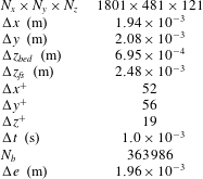
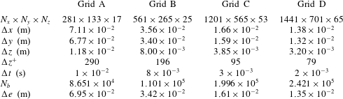
The computational grid system and the time step used for barchan dune simulation. Here,
 $N_{i}$
and
 $\unicode[STIX]{x0394}i$
indicate the number of grid nodes and the grid spacing in the
 $i$
direction respectively;
 $\unicode[STIX]{x0394}x$
and
 $\unicode[STIX]{x0394}y$
represent the grid spacing of the background mesh in the streamwise and spanwise directions respectively. The grid system is uniform in the streamwise (
 $x$
) and spanwise (
 $y$
) directions, while it is stretched in the vertical (
 $z$
) direction. The term
 $\unicode[STIX]{x0394}z_{bed}$
is the grid spacing in the vertical direction near the initial flat bed. The vertical grid spacing in the near-bed zone is uniform, while above this zone (which is 7 cm thick) it is stretched in the vertical direction with a tanh function. The term
 $\unicode[STIX]{x0394}z_{fs}$
is the grid spacing in the vertical direction near the water surface. Thus, the vertical grid spacing varies from a minimum of
 $\unicode[STIX]{x0394}z_{bed}$
to a maximum of
 $\unicode[STIX]{x0394}z_{fs}$
at the water free surface. The terms
 $\unicode[STIX]{x0394}x^{+}$
,
 $\unicode[STIX]{x0394}y^{+}$
and
 $\unicode[STIX]{x0394}z^{+}$
represent the minimum grid spacing in the streamwise, spanwise and vertical directions respectively, scaled in inner wall units. Finally,
 $N_{b}$
is the number of nodes used to discretize the unstructured triangular mesh at the fluid/sediment interface and
 $\unicode[STIX]{x0394}e$
is the average grid spacing of the unstructured triangular mesh.

The fluid/sediment interface is discretized with an unstructured triangular mesh consisting of 363 986 cells (see figure 6). The triangles of the unstructured grid system are of roughly uniform size throughout the mobile bed, with edge sizes ranging from
 $1.7\times 10^{-3}~\text{m}$
to
 $2.1\times 10^{-3}~\text{m}$
. The channel within which the fluid/sediment interface is immersed is discretized with a background Cartesian grid. The background grid consists of 1801, 481 and 121 grid nodes in the streamwise, spanwise and vertical directions respectively (i.e. a total of nearly 105 million nodes). The computational nodes are uniformly spaced in the streamwise and spanwise directions, while they are slightly stretched in the vertical direction. The minimum distance for the first node off the bed in the background grid system is approximately equal to 19 wall units. The details of the grid system we used in this simulation are summarized in table 1. The computational time step is set to 1 ms to ensure the temporal accuracy of the simulation. As an indication of the computational requirements, we note that the coupled simulation on this grid system required 75 days of execution time on 512 c.p.u.s to simulate approximately 3 h of physical time. It is noteworthy to mention that the CURVIB method we employ in this work requires that the background and unstructured triangular grid systems are comparable in terms of grid size. This requirement is to ensure that the flow field quantities are correctly projected onto the fluid/sediment interface. As we have previously shown (see Khosronejad et al.
Reference Khosronejad, Kozarek and Sotiropoulos2014), disparity between the resolution of the two grid systems may lead to stability problems.
The grid sensitivity of the simulation results to the grid resolution we employ herein has already been demonstrated in Khosronejad & Sotiropoulos (Reference Khosronejad and Sotiropoulos2014). In that study, we performed coupled hydro–morphodynamic simulations on four different grid systems denoted as A, B, C and D with
 $22.6$
,
 $30.7$
,
 $42.7$
and
 $79.9$
million grid nodes and corresponding grid resolutions (in wall units) of 40, 30, 23 and 20 respectively. As we showed in Khosronejad & Sotiropoulos (Reference Khosronejad and Sotiropoulos2014), grids A and B were not fine enough to resolve the early stages of bed evolution with regard to both the time scales and the sharpness and clarity of bed features observed in the experiments of Venditti & Church (Reference Venditti and Church2005). However, simulations on grids C and D yielded quite similar results for the initial stage of sand wave development. We note that the grid system we employ in this work – with
 $104.8$
million grid nodes and a corresponding grid resolution (in wall units) of 19 – is even finer that the grid D used in Khosronejad & Sotiropoulos (Reference Khosronejad and Sotiropoulos2014). Therefore, we feel confident that the results we report herein are insensitive to further grid refinement.
4 Simulation results and discussion
The morphodynamic model is activated at
 $t=0$
when the initial flow corresponds to an instantaneous realization of fully developed open channel flow over a rigid bed and there is no suspended sediment present in the flow. Therefore, and as we also found in Khosronejad & Sotiropoulos (Reference Khosronejad and Sotiropoulos2014), the initial bed deformation is driven by the action of turbulent sweep motions near the bed, which transport high-momentum fluid towards the bed and create randomly distributed regions of high shear stress fluctuations. In response to the fluctuating shear stress, cross-hatch patterns appear spontaneously on the entire mobile bed surface, consisting of oblique linear striations with an amplitude of approximately
 $2d_{50}$
and a wavelength of approximately
 $6~\text{cm}$
, as also observed in laboratory experiments (Venditti & Church Reference Venditti and Church2005; Khosronejad & Sotiropoulos Reference Khosronejad and Sotiropoulos2014). These cross-hatch features migrate downstream, leading to the formation of chevron-shaped defects at the nodes of the cross-hatch. The thus-emerging chevron nodes, however, do not all have the same amount of mass since they have been created by local microscour and microdeposition events driven by bed shear stress fluctuations of varying intensity. As a result, smaller nodes travel slightly faster than their somewhat larger neighbours and ultimately catch up with them, merging to form larger sediment nodes. In Khosronejad & Sotiropoulos (Reference Khosronejad and Sotiropoulos2014), the continuous recirculation of sediment provides enough material for transverse dunes spanning the entire width of the channel to ultimately emerge. For the present case, on the other hand, the scarcity of available material causes isolated sediment nodes to grow up to a point and ultimately form barchans, as discussed below.
4.1 Initiation of barchan formation
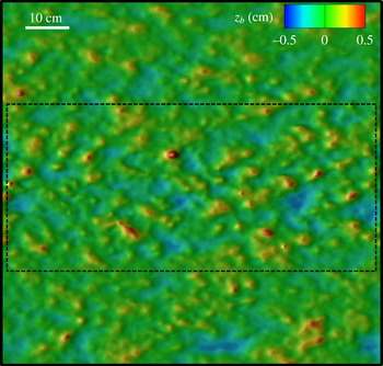
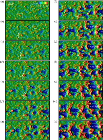
In order to illustrate our findings regarding the collision of sediment masses, we focus our attention on the middle of the flume shown in figure 7 and choose a small window in this area (see the black dashed line in figure 7) to follow the development of small sediment nodes in that area. Subsequent snapshots of the simulated bed elevations from the dashed-line area in figure 7 are shown in figure 8, where we illustrate how the process of fast-moving small sand nodes colliding and merging with larger slower-moving neighbours continues until the first barchanoids emerge on the bed. Starting from
 $t=300~\text{s}$
(figure 8
a), a specific node is marked with a large white circle. In the subsequent figure at
 $t=400~\text{s}$
(i.e. figure 8
b), the large circle depicts the new location of the chevron node, while its location at earlier times is shown with a small white circle. This marking is done for all instants in time shown in this figure as the chevron node becomes larger and eventually forms a crescent-shaped barchanoid. Since the time step between each of the figures is constant and equal to
 $100~\text{s}$
, the spacing of the small white circles can be used to readily estimate the temporal evolution of the speed at which the growing-in-size node migrates. It is evident from figure 8(n) that the process of attracting small fast-travelling sediment masses ultimately leads to a progressively larger and slower-travelling barchanoid. The initiation process of barchans can also be seen in supplementary movie 1 available at https://doi.org/10.1017/jfm.2016.880, rendered from instantaneous snapshots of our simulation results for the bed evolution. It should be noted that the time in movie 1 is approximately 100 times faster than physical time.
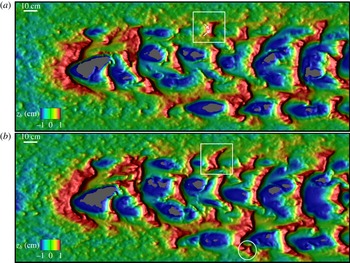
The aforementioned collision and merging process occurs continuously and provides the fundamental mechanisms for the growth and evolution of the barchan field during the early stages of the bed evolution. In figure 9, which depicts the barchan field at two instants of
 $t=5000$
and
 $5500~\text{s}$
, one can readily see multiple collision events underway. This figure also shows the ability of the simulation to capture regions of bedrock that have been exposed on the lee side of the dunes and the onset of surface transverse waves on the windward side of the barchans (see also movie 1). We note that the captured bedrock exposure events are qualitatively similar to those observed in the natural settings shown in figure 1 (for quantitative comparisons, see appendix A). In addition, one can readily pinpoint numerous collision processes in figure 9 that are numerically captured. For example, one can note the collision of small-scale dunes with larger ones shown in the white square in figure 9(a). In figure 1(e), we plot an instantaneous snapshot of experimentally observed subaqueous barchans (Mantz Reference Mantz1978) at their quasiequilibrium, which are stunningly similar to those we have numerically captured (figures 8
j–n and 9).
Simulated genesis of barchans. Three-dimensional plots of bed elevations (
 $z_{b}$
) in a window as wide as the flume and in the middle of it at
 $t=300~\text{s}$
. The dashed lines show the rectangular window in the middle of the channel we have selected to present the simulated bed morphology in figure 8. Flow is from left to right.

Simulated genesis of barchans. Three-dimensional plots of bed elevations (
 $z_{b}$
) in the window shown by the dashed line in figure 7 corresponding to (a)
 $t=300$
, (b)
 $400$
, (c)
 $500$
, (d)
 $600$
, (e)
 $700$
, (f)
 $800$
, (g)
 $900$
, (h)
 $1000$
, (i)
 $1100$
, (j)
 $1200$
, (k)
 $1300$
, (l)
 $1400$
, (m)
 $1500$
and (n)
 $1600~\text{s}$
. The small grey areas in (l–n) show the exposure of bed rock. The large circles and rectangles track the time evolution of two initially small nodes towards larger bed features. Arrows mark small nodes about to merge with larger bed features. The small circles in (b–h) mark the location of the bed feature tracked by the large circle at previous instants in time. Flow is from left to right.

Simulated barchan field after (a)
 $t=5000$
and (b)
 $5500~\text{s}$
. Three-dimensional bed elevation contours (
 $z_{b}$
) are shown in the entire width of the flume and in the middle of its length. The grey areas show the exposure of bed rock. Flow is from left to right.

Simulated calving process. Three-dimensional plots of bed elevations (
 $z_{b}$
) are shown in a selected window in the middle of the channel at (a)
 $t=6800$
, (b)
 $7000$
, (c)
 $7200$
, (d)
 $7400$
, (e)
 $7600$
, (f)
 $7800$
, (g)
 $8050$
, (h)
 $8200$
and (i)
 $8400~\text{s}$
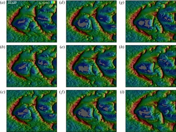
. The morphodynamic unstructured triangular grid for discretizing the bed is shown in black. The grey areas show the exposed bedrock, and flow is from left to right.

4.2 Calving of new barchans
If the process of smaller faster-travelling dunes colliding and merging with larger slower-moving barchans were to continue, one would reasonably expect that the equilibrium state of the process would be a single mega-barchan dune. Our simulations as well as numerous field observations (Hersen et al.
Reference Hersen, Douady and Andreotti2002; Andreotti et al.
Reference Andreotti, Fourriere, Ould-Kaddour, Murray and Claudin2009) clearly show that this is not the case and instead an equilibrium field develops consisting of equilibrium sized as well as a range of smaller barchan dunes – in our simulations the equilibrium height is approximately 5–7 cm, i.e. approximately 40 %–45 % of the flow depth. As pointed out by Elbelrhiti et al. (Reference Elbelrhiti, Claudin and Andreotti2005), for equilibrium to be established, calving is essential, as it provides the sand-loss mechanism that prevents barchan dunes from growing indefinitely. Elbelrhiti et al. (Reference Elbelrhiti, Claudin and Andreotti2005) argued that surface waves on the windward side of the barchans, which essentially are transverse dunes migrating towards the dune horns, are critical for calving to occur. The consecutive snapshots of the simulated equilibrium barchan field (
 $6800~\text{s}<t<8400~\text{s}$
) we show in figure 10 provide conclusive evidence about the linkages between surface transverse waves and calving and reveal the entire process with clarity. For a continuous display of simulation results for the morphological development of a barchan field, the reader is referred to movie 1.
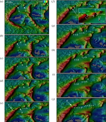
In order to better delineate the calving process observed in our simulations (figure 10), in figure 11 we focus our attention on only half of the barchan field and analyse its development during
 $6800~\text{s}<t<8600~\text{s}$
. At
 $t=6800~\text{s}$
(figure 11
a), a new small barchan ‘b’ is just about to be shed from the horn of the large parent barchan, while another small barchan ‘a’ that was created at an earlier time is already migrating away from the horn. This calving process is continuous, as
 $200~\text{s}$
later yet another dune (‘c’ in figure 11
b) is born. Since these newly born dunes are small, they are able to move faster than and migrate away from their equilibrium-size parent. As shown in figure 11, the amplitude of a newly born barchan is comparable to that of the transverse sand wave at the end of the barchan horn (its parent dune). The width of the newly born barchan, however, is comparable to the width of the barchan horn near its end. For example, see the dot–dash window in figure 11(f), which shows a zoomed-in 3D view of the end point of the barchan horn, where the amplitude and width of the newly born barchan are comparable to those of the parent barchan. Furthermore, these new dunes are not all of equal size and they themselves migrate with variable speed as they begin to interact with their surroundings and attract smaller idle sand patches. As a result, dunes ‘b’ and ‘c’ are seen to merge together in figure 11(e) and at a later time catch up and merge with the leading dune ‘a’ (figure 11
h–j), which by that time has grown considerably and its propagation speed has diminished. Throughout this time, calving of new dunes continues from the horn of the slow-moving parent dune (see new dunes ‘d’, ‘e’ and ‘f’ in figure 11
e–j), and these newly born dunes engage in the same collision and merging interactions as they interact with their surroundings. It is evident, therefore, that both the calving and collision processes are essential mechanisms for an equilibrium dune field to be sustained. Calving provides the sand-loss mechanism that is critical for limiting the size of large dunes and acts to continuously generate new small dunes. These newly born dunes begin to interact with each other via collision and merging processes and eventually grow to be large enough to start calving new dunes themselves and so sustain the equilibrium barchan field. In order to show the details of the unstructured triangular computational mesh and the topological richness of the simulated barchans, we plot in figure 12 a larger-scale (by a factor of
 ${\sim}3$
) plot of figure 10(h) (which is also partly shown in figure 11
g).
Simulated calving process. Three-dimensional plots of bed elevations (
 $z_{b}$
) are shown in the selected window (white dashed line in (a)) in the middle of the channel at (a)
 $t=6800$
, (b)
 $7000$
, (c)
 $7200$
, (d)
 $7400$
, (e)
 $7600$
, (f)
 $7800$
, (g)
 $8050$
, (h)
 $8200$
, (i)
 $8400$
and (j)
 $8600~\text{s}$
. The morphodynamic unstructured triangular grid for discretizing the bed is shown in black. The grey areas show the exposed bedrock. Flow is from left to right. Lower-case letters (a–f) are used to mark the birth and subsequent evolution of new barchans through calving.

Simulated calving process. Three-dimensional plot of bed elevations (
 $z_{b}$
) at
 $t=8200~\text{s}$
. The morphodynamic unstructured triangular grid (in black) for discretizing the bed can be appreciated in this figure. The grey areas show the exposed bedrock. Flow is from left to right.

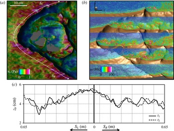
Surface transverse sand waves on the windward side of the dunes are already evident in figure 9 but are very clear in figure 11 and in movie 1 when equilibrium-size dunes have emerged. As the barchans grow towards equilibrium size, they ultimately become large enough to carry a significant amount of sand along their central curved section and horns and also create a major obstacle to the flow in the channel. As the approach flow impinges on the windward side of the barchan, it accelerates as it is diverted sideways and directed towards the horns. The increased shear stress on the curved dune surface (see figure 13
a) destabilizes the sand bed and gives rise to transverse ripples that span the entire windward surface of the barchan. The ripples migrate from the centre of the dune, where sand supply is plentiful, towards the horns, causing the highly irregular wavy surface of the simulated barchan dunes (see figure 13
c). When the surface waves reach the tip of the horn, they destabilize it, causing the shedding of new dunes. To demonstrate the propagation of surface sand waves from the centre towards the two horns, we show in figure 13(c) two consecutive bed elevation profiles plotted along the arclength ‘
 $S$
’ originating at the dune centre and extending towards the horn. The propagation speed of the ripples can also be readily estimated from such plots, and is found to be of the order of
 $0.062~\text{cm}~\text{s}^{-1}$
. We note that this speed is almost an order of magnitude larger than the propagation speed of the large equilibrium barchan (
 $0.0085~\text{cm}~\text{s}^{-1}$
) on the surface of which these ripples migrate. Given the celerity (
 ${\sim}0.062~\text{cm}~\text{s}^{-1}$
) and wavelength of the transverse sand waves (
 ${\sim}15~\text{cm}$
) migrating over the barchan horn near its end, as shown in figure 13(c), every
 ${\sim}300~\text{s}$
one transverse dune reaches the end of the barchan horn. If these transverse surface sand waves reaching the end of the parent barchan horn give rise to the calving of new barchans as we hypothesized in this work, then we should expect to observe a new barchan calving approximately every
 $300~\text{s}$
. As we showed in figure 11, this is exactly what happens during the simulated calving process. Almost every
 $300~\text{s}$
one new barchan is calved at the end of the two horns of the equilibrium barchan. For the same reason, the distance between the two newly born barchans is initially equal to approximately one wavelength of the transverse sand waves (see figure 11).
Simulated instantaneous flow fields and surface waves for a selected barchan at equilibrium (
 $t=10\,600~\text{s}$
). (a) Contours of bed shear stress, (b) contours of instantaneous vorticity magnitude at five
 $y$
 $=$
constant planes and (c) bed profiles along the arclength
 $S$
defined with a white dashed line in (a) showing migrating sand waves over the barchans at
 $t_{1}=10\,300~\text{s}$
and
 $t_{2}=10\,500~\text{s}$
. The grey areas show the exposed bedrock. Flow is from left to right.

Another significant feature of barchan morphology that is evident from figure 13 (see also figures 10 and 11) is the presence of large and topologically complex regions of bedrock exposed on the lee side of the barchan dunes like those observed in natural barchan fields (see the dashed-line area in figure 1 d). To elucidate the mechanism that leads to the exposure of bedrock, we plot in figure 13(b) a snapshot of the instantaneous vorticity field on select vertical slices through the barchan field. This plot reveals a number of important physical mechanisms highlighting the coupling between dune morphology and the turbulent flow. First, the mechanism causing the dune to migrate forward is clearly evident. Along the windward side of the dune, the high-vorticity layer remains attached to the surface because of the acceleration of the approach flow. The shear stress increases and the windward side erodes. Off the barchan slip surface, however, the flow separates and an intense and highly energetic shear layer is created, delineating the high-speed flow above the dune from the low-speed flow on the lee side. The sand that was transported over the dune surface is deposited onto the lee side due to the low velocity in this region, causing the dune to gradually move forward. The shear layer, however, is clearly seen to reattach to the bed on the lee side of the dune. At the attachment point, high-momentum fluid impinges on the bed and causes a near-bed flow directed away from the point of attachment. This near-wall flow is responsible for sweeping material away from the point of attachment and gives rise to the pockets of exposed bedrock. The shapes of the exposed bedrock are found to be very complex and change continuously as a result of the large-scale unsteadiness of the energetic coherent structures that develop in the separate flow off the dune slip surface and the complex topography of the emerging barchan field. This finding is consistent with the numerical observations of Omidyeganeh et al. (Reference Omidyeganeh, Piomelli, Christensen and Best2013), who carried out LES of the turbulent flow over a frozen single barchan. Omidyeganeh et al. (Reference Omidyeganeh, Piomelli, Christensen and Best2013) showed that the asymmetric geometry of the barchan induces energetic vortical structures, which in turn create downwash motions with strong sweep events near the reattachment region.
In order to further elucidate the aforementioned processes by which the bedrock exposure occurs and also show the beauty and at the same time the complexity of the flow and bed interaction, we used our simulation data to render movies 2 and 3. In movie 2, we plot the 3D geometry of the evolving bed, which is coloured with contours of dimensionless shear velocity along with vectors of bedload flux. In movie 3, we show isosurfaces of dimensionless instantaneous vorticity magnitude (
 $\unicode[STIX]{x1D714}(U/H)=25$
, where
 $\unicode[STIX]{x1D714}$
,
 $U$
and
 $H$
are the instantaneous vorticity magnitude in Hz, the bulk velocity in
 $\text{m}~\text{s}^{-1}$
and the mean flow depth in m respectively) over the 3D geometry of the evolving bed. Movie 2, near its end, shows how the near-bed flow is responsible for sweeping material away from the point of attachment and exposure of bedrock. Movie 3, near its end, shows shedding of turbulent coherent structures from the high point of the barchan dune upward. These flow phenomena will be discussed in more detail in Part II of this work, which is currently in preparation.
4.3 Comparisons with laboratory and field measurements
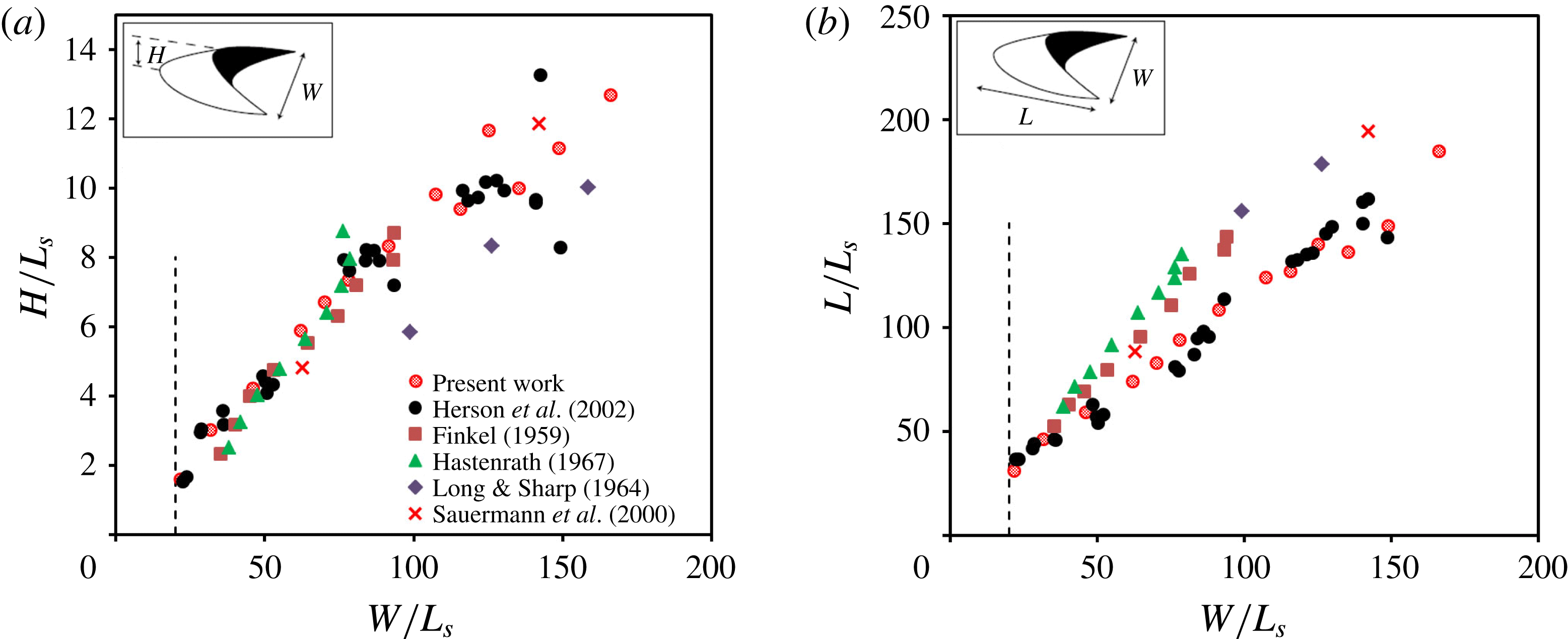
To demonstrate that the dune shapes and sizes we simulate are consistent with those observed in nature and in laboratory settings, we compare in figure 14 simulated and observed non-dimensional dune height
 $H/L_{s}$
and width
 $W/L_{s}$
as functions of the non-dimensional dune length
 $L/L_{s}$
. The computational results shown in figure 14 have been extracted by manually measuring the dimensions of the entire field of simulated barchans at 13 equally spaced instants in time from
 $t=500~\text{s}$
until
 $t=6500~\text{s}$
. At each instant in time, we ensemble average the measured
 $L$
,
 $H$
and
 $W$
values of all individual barchans and plot them in figure 14 along with the measured data from subaqueous and aeolian barchans (Hastenrath Reference Hastenrath1967; Werner Reference Werner1995). It is evident that the computed results are in excellent agreement with observations. Therefore, figure 14 not only demonstrates the accuracy of our simulations but also reinforces the suitability of the saturation length as the proper length scale for subaqueous and aeolian dunes. It should be noted that the data shown in figure 14 include dunes with physical dimensions ranging from tens of centimetres (present case and Hersen et al. (Reference Hersen, Douady and Andreotti2002)) to hundreds of metres (Long & Sharp Reference Long and Sharp1964). By comparing various data points in figure 14, one can clearly see that our simulation results are in better agreement with the experimental data of Hersen et al. (Reference Hersen, Douady and Andreotti2002). We argue that this is due to fact that both investigations focus on laboratory-scale subaqueous barchans. The data sets in figure 14(b) suggesting greater slopes are obtained from large-scale aeolian barchan dunes. Furthermore, there is an apparent deviation in the data points of Long & Sharp (Reference Long and Sharp1964) (figure 14
a). Long & Sharp (Reference Long and Sharp1964) gathered their field data by measuring the characteristics of four single barchans within a barchan field with many dunes in Imperial Valley, CA, USA. The limited number of barchan dunes in their study may play a key role in the deviation of their data points from others.
Morphological characteristics of simulated and measured (Finkel Reference Finkel1959; Long & Sharp Reference Long and Sharp1964; Hastenrath Reference Hastenrath1967; Werner Reference Werner1995; Anderson Reference Anderson1996; Werner Reference Werner1999; Sauermann et al.
Reference Sauermann, Rognon, Poliakov and Herrmann2000; Hersen, Douady & Andreotti Reference Hersen, Douady and Andreotti2002) barchan dunes. The barchan length (
 $L$
), width (
 $W$
) and height (
 $H$
) are scaled with the saturation length (
 $L_{s}$
). The minimum width of the observed barchans in all cases is approximately
 $20L_{s}$
, which is shown by the dashed line. It should be noted that the simulated, laboratory and field observed barchans have a width ratio greater than 20. The characteristics of the simulated barchans are obtained at 13 different instants in time starting from
 $t=500~\text{s}$
until 6500 s with a time interval of 500 s. The characteristics of the simulated barchans at each instant are averaged and presented in (a) and (b).

5 Discussion and conclusions
Our simulations reveal underlying physical processes and enable us to examine previous theories and hypotheses proposed in the literature. For example, our simulations along with our previous work for transverse dunes (Khosronejad & Sotiropoulos Reference Khosronejad and Sotiropoulos2014) suggest that the genesis of dune fields is governed by the hierarchical process of complexity in natural landforms described by Werner (Reference Werner1995) and Werner (Reference Werner1999): fast variables (fast motion of small sediment nodes and turbulent flow physics) slaved to slow variables (the slow motion of larger dunes) ultimately losing their status as independent variables of the system. Figure 8 and movie 1 clearly show how this fundamental process via which fast-travelling small sand nodes collide and merge with slower-travelling larger neighbours biases the evolution of the system towards large equilibrium sized dunes. For this process to work, however, an initial condition should be established at the start of bed evolution consisting of randomly distributed small sand nodes of varying mass size. Our simulations show (see also Anderson (Reference Anderson1996) and Werner (Reference Werner1999)) that this condition is quickly established on the initially flat sand bed as a result of the action of turbulent sweep motions in the vicinity of the bed which give rise to a fluctuating bed shear stress field, which drives local microscour and associated microdeposition events of varying intensity. Thus, the initial seeds of emerging large-scale structure in dune fields can be found in the heterogeneous fluctuations of the bed shear stress in the turbulent flow above the bed. Moreover, this process is identical in the genesis of both transverse and barchan dune fields because the factor of adequate or inadequate sand supply, which ultimately governs the specific dune morphology that will emerge, becomes significant at later times of bed evolution.
Our simulation results provide conclusive evidence that the transverse sand waves migrating over the two horns of the barchan dune give rise to a calving process. The computed celerity and wavelength of the transverse sand waves dictate the frequency of the barchan birth or calving at the end of the parent barchan horn. More specifically, we showed that the wavelength and celerity of the simulated transverse sand waves migrating over the barchan horn near its end are
 ${\sim}15~\text{cm}$
and
 ${\sim}0.062~\text{cm}~\text{s}^{-1}$
respectively (see figure 13
c). These quantities would dictate a barchan birth rate of one every
 ${\sim}300~\text{s}$
. The simulation results shown in figure 11 illustrate approximately the same birth rate (i.e. one every
 ${\sim}300~\text{s}$
). Furthermore, we showed in figure 11(f) that the width and amplitude of the newly born barchans are almost identical to those of the transverse sand waves near the end of the barchan horn. It is also evident from figure 11 that the distance between the newly calved barchans is the same as the wavelength of the transverse sand waves near the end of the barchan horn. All of this quantitative evidence clearly shows for the first time that sand waves on the surface of parent barchan dunes give rise to calving and provide the mechanism for sand loss that sustains barchan fields.
Past studies have emphasized the importance of dune collisions and associated sand exchange mechanisms as the fundamental processes for redistributing sand and preventing the growth of excessively large dunes (Werner Reference Werner1995; Genois et al. Reference Genois, Hersen, du Pont and Grgoire2013). Other studies (Werner Reference Werner1999; Worman et al. Reference Worman, Murray, Littlewood, Andreotti and Claudin2013) have emphasized the importance of calving as the key mechanism for sand loss in large barchans, which is essential for an equilibrium barchan field to be established and sustained. The field observations of Hersen et al. (Reference Hersen, Douady and Andreotti2002) further showed how sand waves on the windward side of the dunes provide the key mechanism for destabilizing the barchan horns and initiating the calving process. Our simulations clearly show that these are not either/or mechanisms but rather parts of a continuum sequence of nonlinear coupled phenomena that all combine in different stages of the process and across a range of scales to give rise to the complexity of barchan fields observed in nature. Surface waves emerge when barchans have grown sufficiently large to modify the flow around them. These waves migrate towards the horns and act to destabilize large barchans, causing calving, which in turn leads to the birth of new barchans of varying sizes and varying propagation speed, which then collide and merge with their neighbours via processes governed by the hierarchical-interaction model of Werner (Reference Werner1999). Our simulations, however, do not support the solitary wave behaviour of dunes proposed by Schwammle & Herrmann (Reference Schwammle and Herrmann2003).
Finally, we note that the computational data sets we have created via our simulations provide a rich database that can be mined to extract quantitative information about the flow, bed morphodynamics and their coupling at various stages of the process. Such information can be used to further examine proposed theories, assess existing and uncover new scaling laws, and develop improved reduced-order models of dune formation. In Part II of this study, we will focus on the simulated flow fields to further elucidate the dynamics of energetic vortical flow structures and their interactions with the mobile bed during various stages of barchan field evolution.
Acknowledgements
This work was partially supported by the National Science Foundation grant IIP-1318201. Computational resources were provided by the University of Minnesota Supercomputing Institute. For additional information regarding the data generated from these simulations, the reader can contact Professor F. Sotiropoulos via email: fotis.sotiropoulos@stonybrook.edu. The VFS-Rivers model is part of the Virtual Flow Simulator (VFS) suite of computational fluid dynamics solvers developed by the group of Professor F. Sotiropoulos. The code is available as open source and can be downloaded, along with supporting documentation, from https://github.com/SAFL-CFD-Lab/VFS-Rivers.
Supplementary movies
Supplementary movies are available at https://doi.org/10.1017/jfm.2016.880.
Appendix A
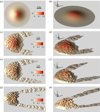
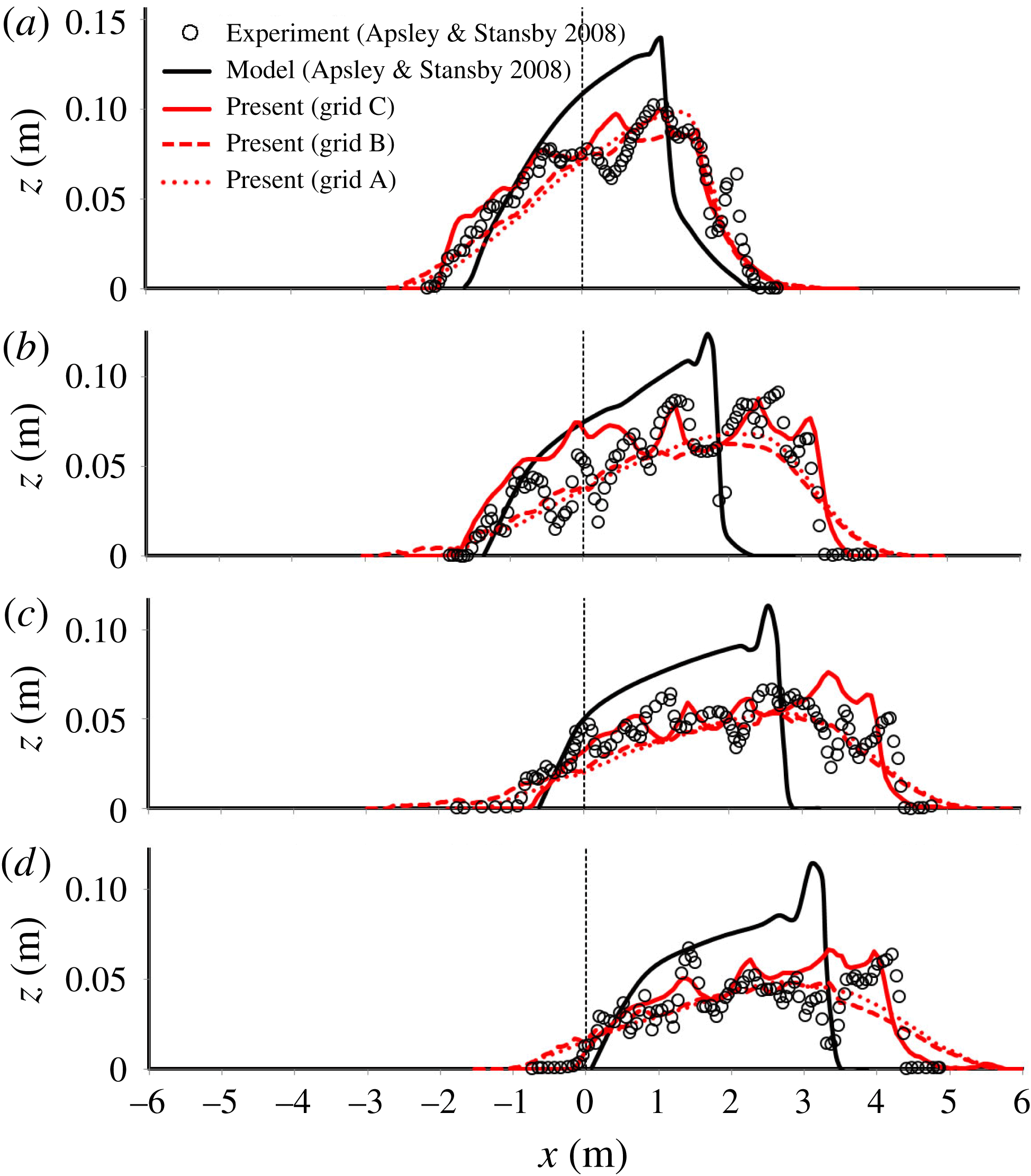
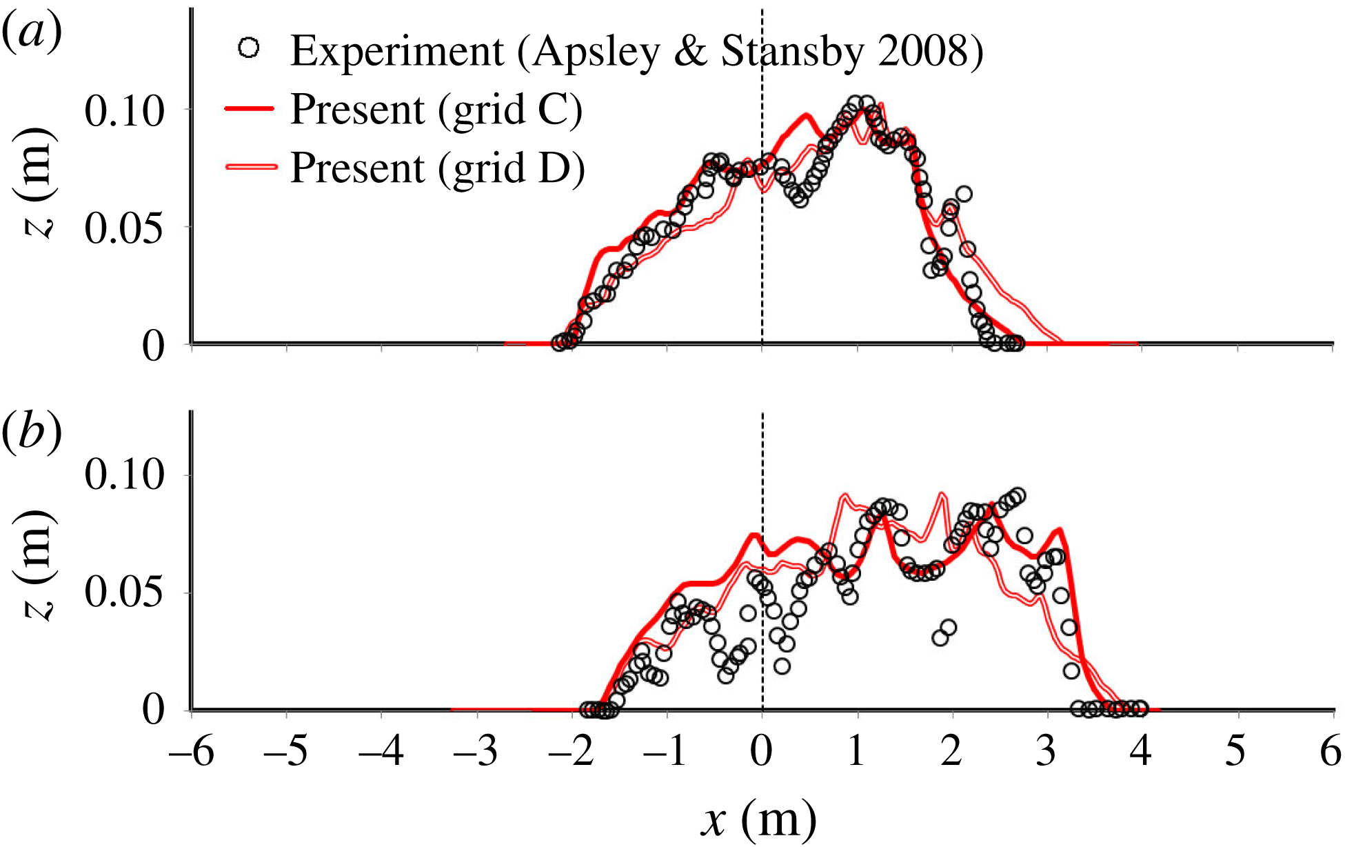
The coupled hydro–morphodynamics model we have employed in this work has been validated previously for transverse sand waves in a laboratory-scale open channel (Khosronejad & Sotiropoulos Reference Khosronejad and Sotiropoulos2014; Sotiropoulos & Khosronejad Reference Sotiropoulos and Khosronejad2016). In this appendix, we present an additional quantitative validation study for a test case that is closely related to the barchan fields we have simulated herein. The test case corresponds to the morphological development of a single subaqueous sand mound under the action of turbulent flow in a rigid flat-bed open channel, which has been studied experimentally and numerically by Apsley & Stansby (Reference Apsley and Stansby2008). In their experiment, Apsley & Stansby (Reference Apsley and Stansby2008) placed an antisymmetric Gaussian sand mound at the centre of a
 $20~\text{m}$
long and
 $9~\text{m}$
wide laboratory flume and allowed it to deform under the action of turbulent channel flow to shape a single barchan. The water flow in their experiment was
 $H=0.2~\text{m}$
deep and had a bulk velocity of
 $U=0.5~\text{m}~\text{s}^{-1}$
(Apsley & Stansby Reference Apsley and Stansby2008). The initial bed elevation (
 $z$
) of the Gaussian sand mound is described by
 $$\begin{eqnarray}z=0.15\text{e}^{-0.693r^{2}},\end{eqnarray}$$
where
 $r$
is the radial distance from the centre of the sand mound. We simulated the experiment of Apsley & Stansby (Reference Apsley and Stansby2008) with three different grid systems with uniform resolution in all directions: (i) grid A with
 ${\sim}0.46$
million computational nodes; (ii) grid B with
 ${\sim}3.7$
million computational nodes, which is obtained by roughly doubling the number of nodes in all directions; (iii) grid C with
 ${\sim}36$
million computational nodes, which is obtained by refining the intermediate grid by a factor of
 $2.1$
in all directions. Details of the three grid systems are shown in table 2. It is worth noting that even the finest grid system (grid C) we employ in this validation case is considerably coarser than the mesh we used for the simulations of barchan fields presented in this paper.
The computational grids and the time steps used for each grid system. Here,
 $N_{i}$
and
 $\unicode[STIX]{x0394}i$
indicate the number of grid nodes and the grid spacing in the
 $i$
direction respectively. The grid systems are uniform in the vertical (
 $z$
), streamwise (
 $x$
) and spanwise (
 $y$
) directions. The term
 $\unicode[STIX]{x0394}z^{+}$
is the minimum grid spacing in the vertical direction scaled in inner wall units;
 $N_{b}$
is the number of nodes used to discretize the unstructured triangular mesh at the fluid/sediment interface;
 $\unicode[STIX]{x0394}e$
is the average grid spacing of the unstructured triangular mesh.

Prior to performing the coupled simulations, we simulated the flow field in the flume without the sand mound being present. In this simulation, we used a periodic boundary condition in the streamwise direction and ran the simulation until a statistically steady fully developed turbulent flow state was reached. The instantaneous realizations of the flow field at the outlet cross-section of the flume were saved and fed as the inlet boundary condition for the coupled flow and bed morphodynamics simulation.
Simulated sand-mound evolution on grid C after (a,b)
 $t=0$
(initial geometry), (c,d)
 $t=10$
min, (e,f) 20 min and (g,h) 60 min in colour scale of the bed elevation (
 $z_{b}(m)$
). In the plan views (a,c,e,g), the flow is from left to right. In the 3D views (b,d,f,h), the flow is along the
 $x$
axis. Vertical coordinates (
 $z$
) are exaggerated by a factor of 4.

Bed elevation of the sand mound along the centreline of the channel after (a) 20 min, (b) 60 min, (c) 120 min and (d) 180 min. The circles and black bold lines represent the experimental and numerical results of Apsley & Stansby (Reference Apsley and Stansby2008) respectively. The red bold, dotted and dashed lines represent the current simulation results with grid systems A, B and C respectively.

Like the experiment of Apsley & Stansby (Reference Apsley and Stansby2008), we start the coupled flow and bed morphodynamic simulations from an initial Gaussian geometry described by the aforementioned (A 1) (see also figure 15
a,b). In figure 15, we show plane and 3D plots of the simulated sand-mound evolution at four different instants in time,
 $t=0$
,
 $t=10$
min,
 $20$
min and
 $60$
min, simulated on the grid C. As shown in this figure, soon after starting the flow, the sand mound starts to evolve and quickly deviates from its initial Gaussian geometry, assuming a barchan-dune-like shape. One readily apparent feature from figure 15 is the emergence of transverse sand waves on the stoss side of the dune, which propagate towards the horns. These transverse sand waves transport the sediment mass over the sand mound towards the two side horns. The thus-transported sediment mass is seen in figure 15 to form two streets of dune calving where masses of sediment detach from the sand mound and migrate downstream (see figure 15
c–h). Therefore, even in this relatively simple generic system, the key mechanisms we discussed extensively in this paper and which have been previously reported in field studies are also observed, namely transverse sand waves transporting sediment towards the dune horns, leading to calving and providing the mechanism for the barchan to lose sand.
In figure 16, we compare our simulation results on the three grid systems with the measurements and numerical simulations of Apsley & Stansby (Reference Apsley and Stansby2008) at the centreline of the channel for the instantaneous bed elevations at time instants of
 $t=20$
min,
 $60$
min,
 $120$
min and
 $180$
min. We note that Apsley & Stansby (Reference Apsley and Stansby2008) employed a Reynolds-averaged model in their simulations on a rather coarse (
 ${\sim}100\,000$
nodes) body-fitted grid. As shown in figure 16, our simulated results on all three grid systems represent a major improvement when compared with the predictions of Apsley & Stansby (Reference Apsley and Stansby2008). Namely, our model is able to capture correctly the dynamic evolution of the sand mound general shape and its migration speed. The experiments, however, do show that the shape of the mound is not smooth but is rather dominated by surface sand waves throughout its evolution. As seen in figure 16, only grid C, resolving more accurately the details of the near-bed turbulent flow, is able to capture this important feature of the morphodynamics.
Our simulation results on grid C (figure 16) clearly show that the transverse surface sand waves migrate over the sand mound with similar amplitude (
 $1$
–
 $5~\text{cm}$
) and wavelength (
 $0.5$
–
 $1.5~\text{m}$
) to those observed experimentally. Similarities between the measured and numerically captured surface sand waves migrating over the main sand mound aside, one apparent discrepancy is that the two do appear to be out phase. This is to be expected since it is not straightforward to synchronize instantaneous images of such a dynamically rich morphodynamic evolution.
Apsley & Stansby (Reference Apsley and Stansby2008) did not discuss the origin of the surface sand waves appearing on the profiles of bed elevation in their measurements. The results we have shown in figure 16, however, along with our previous discussion in this paper, clearly show that these wavy bed elevation profiles are the result of transverse sand waves on the stoss surface of the barchan-like dune that transport masses of sand from the centre of the sand mound towards the horns. The numerical simulations of transverse sand waves on barchan dunes and their role in sustaining quasiequilibrium of dunes fields are major contributions of this work. Therefore, the results we present herein validate the ability of our method to accurately simulate such phenomena. Furthermore, they provide new physical insights into the experiment of Apsley & Stansby (Reference Apsley and Stansby2008).
Bed elevation of the sand mound along the centreline of the channel after (a) 20 min and (b) 60 min. The circles, red bold line and red double line represent the experimental results of Apsley & Stansby (Reference Apsley and Stansby2008) and the current numerical results with grid systems C and D respectively.

To make sure that our simulated bed morphology on grid C is independent of the grid size, we conducted yet another simulation on an even finer (than grid C) grid system, which is denoted as grid D. As shown in table 2, grid D consists of
 $1441\times 701\times 65$
nodes, which results in a grid resolution of
 $1.384\times 10^{-2}~\text{m}$
,
 $1.325\times 10^{-2}~\text{m}$
and
 $3.2\times 10^{-3}~\text{m}$
in the streamwise, spanwise and vertical directions respectively, with a temporal step of
 ${\sim}2~\text{ms}$
. The average grid spacing for the unstructured triangular mesh in this simulation is
 $1.351\times 10^{-2}~\text{m}$
. Due to the excessive computational cost of this very fine simulation, we only continued the simulation for 60 min. In figure 17, we compare the measured and simulated sand-mound evolution along the centreline of the channel. The comparison presented in this figure shows a similar trend for the simulation results on the two finest grid systems (grids C and D), pointing to the conclusion that both simulations are able to capture the dynamics of the large eddies that drive sand-mound movement and transverse surface sand-wave evolution.