Introduction
Antarctic palaeoclimate data are available not only from deep ice cores but also from the surface of Antarctic blue ice areas (BIAs). Many of these BIAs are known to have very old ice at the surface (Whillans & Cassidy Reference Whillans and Cassidy1983, Bintanja Reference Bintanja1999). The surface blue ice can also provide higher temporal resolution than usual in deep ice cores (Moore et al. Reference Moore, Nishio, Fujita, Narita, Pasteur, Grinsted, Sinisalo and Maeno2006, Sinisalo et al. Reference Sinisalo, Grinsted, Moore, Meijer, Martma and van De Wal2007), and BIAs are often located in coastal and mountainous areas where deep cores are not currently available. Thus, a series of shallow cores or samples from a horizontal surface transects from BIAs may complement the deep ice core insight of climate history (Custer Reference Custer2006, Moore et al. Reference Moore, Nishio, Fujita, Narita, Pasteur, Grinsted, Sinisalo and Maeno2006, Sinisalo et al. Reference Sinisalo, Grinsted, Moore, Meijer, Martma and van De Wal2007, Popp et al. unpublished).
The first scientific description of an Antarctic BIA was given by Schytt (Reference Schytt1961) though there is a good general introduction by Giaever (Reference Giaever1954) concerning the first expedition to visit a BIA. The expedition members discovered the amazing stability of the snow-blue ice boundary by placing matchsticks at the boundary - many of which were still in place and not buried several months later. Schytt (Reference Schytt1961) noted that crystal size of the blue ice indicated a deep source for the ice. Crary & Wilson (Reference Crary and Wilson1961) first described the surface characteristics of BIA and discussed formation of BIAs by horizontal compressive forces with katabatic winds removing snow accumulation. Much of the early scientific interest in Antarctic BIAs was due to their nature as meteorite collectors (Cassidy et al. Reference Cassidy, Olsen and Yanai1977, Whillans & Cassidy Reference Whillans and Cassidy1983, Nishiizumi et al. Reference Nishiizumi, Elmore and Kubik1989). The initial discovery of meteorites was made in the South Yamato BIA (Fig. 1) by Yoshida et al. (Reference Yoshida, Ando, Omoto, Naruse and Ageta1971) in 1969. Since then, more than 25 000 meteorites have been found on Antarctic BIAs (Harvey Reference Harvey2003). Consequently, the ice flow regime was studied and ice flow models were published for several BIAs to explain the meteorite findings (Naruse & Hashimoto Reference Naruse and Hashimoto1982, Whillans & Cassidy Reference Whillans and Cassidy1983, Azuma et al. Reference Azuma, Nakawo, Higashi and Nishio1985). When researchers started to understand the flow regime of the BIAs, they also became interested in the palaeoclimate record stored on the surface of BIAs (Bintanja Reference Bintanja1999, Custer Reference Custer2006, Moore et al. Reference Moore, Nishio, Fujita, Narita, Pasteur, Grinsted, Sinisalo and Maeno2006, Sinisalo et al. Reference Sinisalo, Grinsted, Moore, Meijer, Martma and van De Wal2007, Corti et al. Reference Corti, Zeoli, Belmaggio and Folco2008, Popp et al. unpublished).
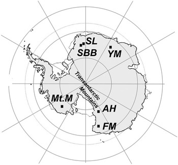
Some Antarctic BIAs of scientific interest. SBB = Scharffenbergbotnen, SL = “Slöret”, YM = Yamato Mountains, Mt.M = Mount Moulton, AH = Allan Hills, FM = Frontier Mountain. Buråsbotnen is located about 50 km north-east from SBB. SBB also indicates the location of Heimefrontfjella mountain range in Dronning Maud Land.

Bintanja (Reference Bintanja1999) stated that the easily recoverable ancient surface ice of the BIAs could be of great value for palaeoclimatic purposes if the dynamics and the internal structure of the Antarctic BIAs were better known. In principle, a simple trench in the surface along a flow line of a BIA would yield ice samples of the full range of ages from present day at the upstream snowline to ice that can be as old as the particular BIA. However, dating surface blue ice is demanding since traditional ice core dating methods cannot be easily applied for BIAs where the ice flow history is often complex and layering not horizontal. Blue ice samples from various BIAs have been dated using the terrestrial ages of meteorites found on their surface (e.g. Whillans & Cassidy Reference Whillans and Cassidy1983, Nishiizumi et al. Reference Nishiizumi, Elmore and Kubik1989), by 14C dating of air trapped in the ice (Van Roijen et al. Reference Van Roijen, van der Borg, de Jong and Oerlemans1995, van der Kemp et al. Reference Van der Kemp, Alderliesten, van der Borg, de Jong, Lamers, Oerlemans, Thomassen and van de Wal2002), by radiometric dating of tephra layers found at the surface of BIAs (Wilch et al. Reference Wilch, Mcintosh and Dunbar1999), by stratigraphical comparison with well-dated ice cores (Moore et al. Reference Moore, Nishio, Fujita, Narita, Pasteur, Grinsted, Sinisalo and Maeno2006), and by combination of several methods (Sinisalo et al. Reference Sinisalo, Grinsted, Moore, Meijer, Martma and van De Wal2007). There are several BIAs, such as South Yamato and Allan Hills, (Fig. 1) where the surface blue ice is estimated to be tens or hundreds of thousands of years old (Whillans & Cassidy Reference Whillans and Cassidy1983, Nishiizumi et al. Reference Nishiizumi, Elmore and Kubik1989, Welten et al. Reference Welten, Nishiizumi and Caffee2000), and the oldest terrestrial ages of meteorites are about 2 millions years. However, there are still only a few palaeoclimate records from BIAs although potentially both the record length and temporal resolution may be higher than those from any of the other Antarctic ice cores.
There are a number of open questions related to the BIAs, for example their general stability under different climate regimes, and the surface age gradient of individual BIAs of interest (Bintanja Reference Bintanja1999). In this paper, we review the latest knowledge of the BIAs emphasizing palaeoclimate applications.
Antarctic blue ice areas (BIAs)
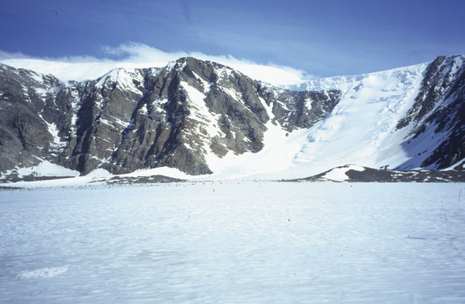
BIAs are bare ice fields (Fig. 2) that the wind keeps clean of snow. Their area can vary from a few hectares, e.g. many small BIAs in coastal mountainous regions of East Antarctica, to thousands of square kilometres, e.g. South Yamato BIA. Blue ice extent may vary because of weather, seasonal effects, and climate change. These changes, however, have not been well quantified.
A BIA in the Scharffenbergbotnen valley surrounded by mountains. (Photo: FINNARP/Anna Sinisalo)

Bintanja (Reference Bintanja1999) defines BIAs as areas where surface mass balance is negative, sublimation forms the main ablation process, and surface albedo is relatively low. This definition of BIAs specifically excludes melt-induced bare ice areas which are located on slopes in coastal areas where climate conditions together with favourable surface orientation favour surface and near-surface seasonal melt (Liston & Winther Reference Liston and Winther2005). These areas were identified by their spectral reflectance signature in satellite imagery by Winther et al. (Reference Winther, Jespersen and Liston2001) who divided observed bare ice regions to melt-induced and wind-induced BIAs. While melt-induced bare ice represents a minority of Antarctic blue ice they are significant in that they are used as water supplies to Antarctic bases. For example, the Finnish and Swedish bases Aboa and Wasa use a melt area at Basen nunatak in Dronning Maud Land. Melt-induced bare ice fields are also used as landing strips for wheeled aircraft such as the runaway close to the Novolazarevskaya Station in Schirmacher Oasis, East Antarctica. For many Antarctic visitors these bare ice regions are their only experience of blue ice, and this often leads to false impressions about Antarctic BIAs. According to the definition sublimation is the dominant ablation mechanism of a BIA, and it is clear that only the wind-induced BIAs can be useful for palaeoclimate studies.
Geographical distribution
BIAs cover about 1% of the Antarctic surface area (Bintanja Reference Bintanja1999). They are scattered widely over the continent appearing mainly in the vicinity of mountain ranges and nunataks as they are likely to form at locations where ice flow is dammed by outcropping nunataks or slowed by sub glacial bedrock ridges (e.g. Faure & Buchanan Reference Faure and Buchanan1991), precipitation is low and the annual mean wind speed relatively high (Van den Broeke & Bintanja Reference Van den Broeke and Bintanja1995). These phenomena explain why Antarctica is the only place on Earth where BIAs exist.
Only a few BIAs have been studied in detail. They are located (Fig. 1) in the vicinity of South Yamato Mountains (e.g. Naruse & Hashimoto Reference Naruse and Hashimoto1982, Azuma et al. Reference Azuma, Nakawo, Higashi and Nishio1985, Moore et al. Reference Moore, Nishio, Fujita, Narita, Pasteur, Grinsted, Sinisalo and Maeno2006), the Allan Hills (e.g. Schultz et al. Reference Schultz, Annexstad and Delisle1990, Faure & Buchanan Reference Faure and Buchanan1991, Spikes Reference Spikes2000), Mount Moulton (e.g. Wilch et al. Reference Wilch, Mcintosh and Dunbar1999, Dunbar et al. Reference Dunbar, Mcintosh and Esser2008), and Heimefrontfjella mountain range in Dronning Maud Land (e.g. Bintanja Reference Bintanja1999, Sinisalo Reference Sinisalo2007). In addition, other BIAs, such as Frontier Mountain BIA (Perchiazzi et al. Reference Perchiazzi, Folco and Mellini1999) have been studied less intensively (Fig. 1), and many have simply been utilized as meteorite stranding grounds (e.g. Welten et al. Reference Welten, Nishiizumi and Caffee2000). Palaeoclimate data have been collected from South Yamato (Nakawo et al. Reference Nakawo, Nagoshi and Mae1988, Machida et al. Reference Machida, Nakazawa, Narita, Fujii, Aoki and Watanabe1996, Moore et al. Reference Moore, Nishio, Fujita, Narita, Pasteur, Grinsted, Sinisalo and Maeno2006), Mount Moulton (Custer Reference Custer2006, Popp et al. unpublished), and Scharffenbergbotnen in the Heimefrontfjella mountain range (Sinisalo et al. Reference Sinisalo, Grinsted, Moore, Meijer, Martma and van De Wal2007).
Ice flow
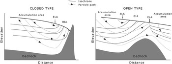
There is a net upward component in the ice flow pattern in BIAs. Thus, old ice layers originally buried deep in firn flow up to the surface and old ice emerges at the surface of the BIA (Fig. 3). The ice flow regime, however, tends to be complex at BIAs due to rough basal topography. This is the case even for large BIAs that extend well upstream of surface outcrops such as South Yamato mountain BIA (e.g. Moore et al. Reference Moore, Nishio, Fujita, Narita, Pasteur, Grinsted, Sinisalo and Maeno2006) and on smaller scales in Allan Hills (Grinsted et al. Reference Grinsted, Moore, Spikes and Sinisalo2003). On the other hand, present-day flow regimes may be simple e.g. Scharffenbergbotnen (Jonsson Reference Jonsson1992, Grinsted et al. Reference Grinsted, Moore, Spikes and Sinisalo2003, Sinisalo et al. Reference Sinisalo, Grinsted and Moore2004, Reference Sinisalo, Grinsted, Moore, Meijer, Martma and van De Wal2007). Flow history may have varied significantly over a glacial/interglacial cycle which makes dating of surface ice more complicated. The surface ice used for palaeoclimate purposes to date varies from the Holocene (Sinisalo Reference Sinisalo2007, Sinisalo et al. Reference Sinisalo, Grinsted, Moore, Meijer, Martma and van De Wal2007) up to about 150 000 years (Popp et al. unpublished).
A sketch of ice flow in a closed type and in an open type (see Classification of blue ice areas for definition) BIA. The flow direction is from left to right. Equilibrium line (ELA) separates the snow covered accumulation area from the ablation area i.e. the BIA. The isochrones that represent individual annual layers come up to the surface of the BIA eventually resulting in near-vertical layering in a closed BIA. The oldest ice layers are found at the surface at the end of the BIA while they may never reach the surface on the open BIA.

Meteorology
The formation and maintenance of BIAs is facilitated by specific meteorological conditions induced by nearby mountains (Bintanja & Van den Broeke Reference Bintanja and van den Broeke1995a, Reference Bintanja and van den Broeke1995b, Bintanja et al. Reference Bintanja, Jonsson and Knap1997, Bintanja & Reijmer Reference Bintanja and Reijmer2001). Meteorological conditions over the BIA differ from those over the snow covered surroundings due to
1) differences in surface characteristics, such as albedo, extinction characteristics for solar radiation, and surface aerodynamic roughness, between blue ice and snow, and
2) differences in topographic setting or nearby orography.
The air over the BIA is warmer and the relative humidity is lower than over a corresponding snow site, and these conditions contribute to significantly higher sublimation rates over BIAs than over snow (Bintanja & Reijmer Reference Bintanja and Reijmer2001). In general and depending on local topography, this can be attributed to adiabatic warming of large-scale katabatic flows (such as descending over much of East Antarctica), aided by diabatic warming due to radiation, and by turbulent mixing of warm air from aloft into the boundary layer (Bintanja & Reijmer Reference Bintanja and Reijmer2001). The surface winds over BIAs are generally gustier than those over adjacent snow fields but the average wind speeds are comparable with each other (Bintanja Reference Bintanja1999).
Surface characteristics
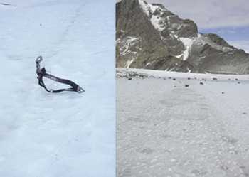
Antarctic BIAs have special surface characteristics such as low albedo, and aerodynamic smoothness in comparison to the surrounding snow and ice covered areas (Bintanja Reference Bintanja1999). These characteristics aid formation and maintenance of the BIAs (Bintanja & Van den Broeke Reference Bintanja and van den Broeke1995a, Reference Bintanja and van den Broeke1995b, Bintanja & Reijmer Reference Bintanja and Reijmer2001). The surface of BIAs is generally rippled (Fig. 4). Bintanja et al. (Reference Bintanja, Reijmer and Hulscher2001) suggest that the only possible mechanism for blue-ice ripple formation is sublimation, occurring whenever there is wind forcing. The orientation of the crests of the ripples is perpendicular to that of the direction of the strongest winds. The measured wave-heights in different BIAs vary between 2 and 10 cm, and the wave-length between 5 and 24 cm (Weller Reference Weller1968, Mellor & Swithinbank Reference Mellor and Swithinbank1989, Bintanja et al. Reference Bintanja, Reijmer and Hulscher2001). The annual average-wave height does not vary over time. The wave-height increases in the summer as the troughs of the ripples experience more sublimation than the crests, but this increase is compensated in winter (Bintanja et al. Reference Bintanja, Reijmer and Hulscher2001). On the other hand, if the seasonal temperatures approach within a few degrees of melting the peaks are smoothed and melt can partially fill the troughs.
Surface characteristics of a BIA. Dust bands can appear as distinct narrow stripes (left) or as more than metre wide bands at the surface of a BIA. Supraglacial moraines and cryoconite holes are visible on the dust band on the right. (Photo: left: FINNARP/Anna Sinisalo, right: FINNARP/Aslak Grinsted)

Dust or tephra bands (Fig. 4) are found in the surface of many BIAs where they usually appear perpendicular to the ice flow (Bintanja Reference Bintanja1999) although the dust bands in the Allan Hills and the Yamato Mountains are reported to curl back as much as 180° in some cases (Koeberl Reference Koeberl1990). In our experience, however, local ice flow directions found by measurements can be quite different from intuitive ideas, and dust bands always appear to be perpendicular to flow, provided that large gradients in ablation rates or large surface elevation changes (relative to the dip angle of dust layers in the ice) are not present.
The origin of visible layers is of great interest. Dust bands in Allan Hills (Nishio et al. Reference Nishio, Katsushima and Ohmae1985), Mount Moulton (Wilch et al. Reference Wilch, Mcintosh and Dunbar1999, Dunbar et al. Reference Dunbar, Mcintosh and Esser2008), South Yamato (Nishio et al. Reference Nishio, Katsushima and Ohmae1985), Frontier Mountain (Perchiazzi et al. Reference Perchiazzi, Folco and Mellini1999) and Lewis Cliff Tongue (Koeberl et al. Reference Koeberl, Yanai, Cassidy and Schutt1988) have been shown to be of volcanic origin (Koeberl Reference Koeberl1990), and may be correlated with individual Pleistocene volcanoes in Antarctic and sub-Antarctic regions. When volcanic eruptions disperse large quantities of ash over Antarctica, the material falls on snow accumulation areas, where it is buried under new snow layers and incorporated in the ice, and is transported to ablation zones. Such dust bands emerging at the surface in BIAs constitute isochronous layers. Sources for soluble and insoluble impurities other than volcanoes include:
1) material from sub glacial bedrock debris scraped up from the ground by the movement of the glacier. In practice this may be very difficult to find given the usual presence of moraines near the mountain terminus of a BIA where the bedrock may accumulate.
2) cosmic particles falling as micrometeorites or meteorite ablation spherules. These are known to constitute a sizable fraction of dust in central east Antarctica regions such as Dome Fuji (Nakamura et al. Reference Nakamura, Imae and Nakai1999), and so may be found in the down-slope flow line outcrop BIA of South Yamato Mountains, and
3) continental and marine dust and aerosols transported by wind. These probably constitute much of the material in the BIA of Dronning Maud Land which is far from active volcanic sources. (Koeberl Reference Koeberl1990)
Banding may also arise due to changes in flow of the ice due to surrounding ice sheet elevation changes incorporating moraine from other inflows, organized cryoconite separation similar to frost-heaving produced stone polygons and stripes, and ogive-like formation due to seasonal changes in flow over an icefall. However, all the mechanisms while possibly explaining some specific bands, cannot explain the general widespread banding on virtually every significant BIA we have observed. The widespread occurrence of bands, and the observation that often only fine grain material is present in them below about ten cm depth also suggest that the bands were formed on the snow surface far from the nunataks. This would mean perhaps up to tens of kilometres from the local nunataks. Hence, it can be assumed that the bands are isochrones and can therefore be reliably used as indicators of ice flow and ablation. Their presence also has implications for general climate conditions that allowed widespread dust covering of the snow surface in the BIA accumulation areas.
Cryoconite holes can be found at the surface of low altitude BIAs (Bintanja Reference Bintanja1999). They indicate melting, which may be purely internal due to solid-state greenhouse effects. The holes are round, bubble-free patches of ice (Fig. 4) that form due to absorption of solar radiation by dark particles or stones, causing their temperature to rise above the melting point (Bintanja Reference Bintanja1999). Small stones and dirt will slowly sink into the ice until a depth where shortwave heating is diminished and equals conductive cooling.
Cryoconite holes are often preferentially formed on the bands on the ice surface. This is most likely due to the slightly lower surface of the band caused by its higher ablation rate allowing windblown rock particles to settle on the ice surface. The coarser cryoconites are confined in the upper decimetre, with only fine grain material beneath it. The abundance of cryoconites can be so significant that it influences the ablation rate of the glacier surface (Takeuchi Reference Takeuchi2002) due to its dark colouration and capacity to absorb solar radiation (Fig. 4). This solid-state greenhouse effect produces a favourable, watery niche for photosynthesis and, thereafter, bacterial respiration and grazing. Here viruses, bacteria (especially cyanobacteria), algae and fungi are typically dominant and they combine to form a soil-like granule (called cryoconite). These biota include organisms up to 105 years old that can be resuscitated and then thrive alongside younger organisms on the ice surface in a so-called supraglacial ecosystem (Hodson et al. Reference Hodson, Mumford, Kohler and Wynn2005).
The depth of cryoconite holes varies seasonally. In winter after wind ablation and no solar heating, dark material is closer to the surface than after the summer when darker material has melted into the ice. On Scharffenbergbotnen, for example, some debris from an old weather station destroyed by high winds can be seen within a few centimetres of the surface before summer begins in November, but by end of January the aluminium parts are 5–8 cm beneath the ice surface. Ablation in cryoconite holes can be a significant practical problem if the bare ice is used as a landing strip for wheeled aircraft. In an effort to improve the ice runway at Troll station, thousands of cryoconite holes were individually cleaned by removing all the cryoconite material from the meltwater in the holes. It is not known how frequently this procedure needs to be repeated as in the long-term as winds from the surrounding nunataks will surely provide more cryoconite raw material.
Snow patches often occur on BIA. While snow is often blown off a BIA, it can persist on the surface for many weeks to several years. The strong radiation, gusty winds and thermal gradients near the surface ice mean that the snow is quickly transformed into hard firn that becomes quite securely attached to the ice surface. However, the violent storms that can sweep BIA seem to be capable of removing even such dense firn from ice surfaces and preserving an ice surface that may be often hidden beneath up to 50 cm of hard-packed snow.
Classification of blue ice areas
BIAs can be classified according to their flow regime (Fig. 3, Grinsted et al. Reference Grinsted, Moore, Spikes and Sinisalo2003) into 1) open type BIAs, and 2) closed type BIAs. This division is relevant to the surface-age distribution of the BIA and hence the palaeoclimate record that can be produced. Flow in an open BIA is not dammed by mountains, nunataks or bedrock topography and ice flows through the BIA. So the oldest layers of ice do not come to the ice surface at all. The dip angles of outcropping isochrones are smaller than at the surface of the closed BIA. Closed BIAs are located at mountain ranges where flow is dammed. The oldest layers of ice will be found in the surface closest to the mountains as if the layers had climbed up the mountain slope (Fig. 3). The South Yamato BIA is the largest open BIA in Antarctica, while e.g. Scharffenbergbotnen is a closed BIA. Locally flow pattern in large open BIA can trap flow in cul-de-sacs and these are where the oldest terrestrial ages of meteorites have been found, particularly in Manhaul Bay in the Allan Hills BIA.
Takahashi et al. (Reference Takahashi, Endoh, Azuma and Meshida1992) classified BIAs into four types based on geographical setting and ice flow characteristics of the BIA. This geographical classification of BIAs was reproduced by Bintanja (Reference Bintanja1999), and it can be useful in understanding the formation and maintenance of a BIA:
1) Type I BIAs are associated with mountains protruding through the ice. They are situated in the lee of an obstacle, which acts as a barrier for snowdrift. The length of these BIAs can be estimated to be roughly 50 to 100 times the height of the obstacle relative to the ice surface (Takahashi et al. Reference Takahashi, Endoh, Azuma and Meshida1992). This is the most common type of BIA (Bintanja Reference Bintanja1999). Scharffenbergbotnen is an example of the type I BIAs
2) Type II BIAs are located on a valley glacier. The descending katabatic winds cause net erosion of the surface and a local divergence of snowdrift, eventually leaving bare blue ice.
3) Type III BIAs are located on relatively steep slopes without mountains protruding through the ice. The increasing surface slope accelerates down slope katabatic winds, causing a divergence of snowdrift transport similar to type II (Takahashi et al. Reference Takahashi, Endoh, Azuma and Meshida1992). The South Yamato mountains BIA is of this type.
4) Type IV BIAs are situated at the lowest part of a glacier basin. Accelerating katabatic winds in the basin remove snow from the surface.
Variability of blue ice extent
The relationship between blue ice extent and climate is not straightforward. Blue ice extent is sensitive to various climatic parameters, and climate change will affect the processes creating blue ice in several ways. Changes in air temperature will affect energy available for surface ablation, and changes in precipitation, and wind velocity will affect accumulation. (Orheim & Lucchitta Reference Orheim and Lucchitta1990)
Large reductions in exposed BIA are more likely than large increases and increasing a BIA can be expected to take a longer time than decreasing it (e.g. Bintanja Reference Bintanja1999, Brown & Scambos Reference Brown and Scambos2004). As a BIA cannot expand onto a nunatak area, aerial increase must take place into adjacent snow fields by the relatively slow processes of either dry snow metamorphosis or exposure of sub-surface ice (Orheim & Lucchitta Reference Orheim and Lucchitta1990). A decrease of the BIA, on the other hand, can happen quickly as a result of increased accumulation or possibly changed wind patterns (Bintanja & Van den Broeke Reference Bintanja and van den Broeke1995a). Seasonal and even annual variations in BIA extent due to snow accumulation events may be large and significant area reductions may occur (Brown & Scambos Reference Brown and Scambos2004). Minimum in the BIA extent is reached in winter (Brown & Scambos Reference Brown and Scambos2004). Snow that accumulates over a long period may be removed rapidly by a large storm. This was observed in Scharffenbergbotnen (Fig. 1) where a severe storm in January 2007 removed old firn and surface snow up to 50 cm thick. There have been attempts to estimate areal changes in individual BIAs (Orheim & Lucchitta Reference Orheim and Lucchitta1990, Spikes Reference Spikes2000, Brown & Scambos Reference Brown and Scambos2004), and the total extent of Antarctic BIAs using satellite images (Winther et al. Reference Winther, Jespersen and Liston2001). Increasing accumulation leading to a general decrease in blue ice can be easily detected, whereas increased ablation is more difficult to observe and requires more permanent change before it will be noticed. Since the possible permanent changes in blue ice extent are very slow and satellite images exist only over the last few decades, no change has been observed that could be interpreted as a climate signal.
When a BIA has formed, it tends to persist due to two conservative feedback processes (Bintanja Reference Bintanja1999). These processes may enable BIAs to persist and possibly expand in the downwind direction. Firstly, the relatively low albedo of the blue ice increases the absorption of solar radiation, which increases the energy available for sublimation. Secondly, the smooth blue ice surface prevents drifting snow from becoming permanently attached, resulting in zero accumulation in the longer term.
Although BIAs seem to be rather stable due to the feedback mechanisms described above, climate change may affect ice flow patterns and even reverse the ice flow direction in some areas. This can have a significant influence on BIA extent over the long-term as ice flow in the BIA will determine how stable a BIA is over glacial-interglacial periods (Bintanja Reference Bintanja1999, Coren et al. Reference Coren, Delisle and Sterzai2003, Sinisalo et al. Reference Sinisalo, Grinsted, Moore, Meijer, Martma and van De Wal2007). Allan Hills, for example, is the location of the oldest know terrestrial age meteorites discovered. However, the existence of very old ice does not necessarily imply a continuous temporal climate record. Coren et al. (Reference Coren, Delisle and Sterzai2003) suggest that the general ice flow has changed its direction in glacial-interglacial cycles in Allan Hills, and the ice with meteorites flows accordingly back and forth across the area. As the ice sheet is thinner in warm periods, open-type BIAs form on the lee side of bedrock rises, and some of the ice may flow back toward these ablation areas allowing meteorite concentrations to increase. In cold periods the regional ice flow is likely to be reduced but the flow is more uniform as the ice sheet is thicker (Coren et al. Reference Coren, Delisle and Sterzai2003).
Changes in ice sheet thickness control the existence of the BIAs in the mountainous areas (Bintanja Reference Bintanja1999, Sinisalo Reference Sinisalo2007). Bintanja (Reference Bintanja1999) suggested that many of the type I BIAs currently existing in Dronning Maud Land did not exist during at LGM. He speculated that the height of the outcropping mountain in comparison to the ice surface height seems to be a critical variable in the temporal variations of type I BIA extent, as a thickening of the ice sheet leading to submergence of a nunatak will tend to make the BIA disappear. Ice sheet elevation changes at the glacial termination are likely to have been most pronounced in the nunatak areas a few hundred kilometres from the coast (Pattyn & Decleir Reference Pattyn and Decleir1998). The surface of the major part of the East Antarctic plateau ice sheet may have been about 100 m lower at LGM than at present (Jouzel et al. Reference Jouzel, Raisbeck, Benoist, Yiou, Lorius, Raynaud, Petit, Barkov, Korotkevitch and Kotlyakov1989, Pattyn Reference Pattyn1999, Ritz et al. Reference Ritz, Rommelaere and Dumas2001) whereas surface elevation at the margins of the plateau, may have been hundreds of metres higher (Näslund et al. Reference Näslund, Fastook and Holmlund2000, Hättestrand & Johansen Reference Hättestrand and Johansen2005). Surface elevation in Scharffenberbotnen, for example, was 200–250 m higher at LGM when surrounding ice sheet flowed in to the valley over its side walls (Hättestrand & Johansen 2005). The surface elevation started to decrease when lowering of the surrounding ice sheet reached a point where the outcropping mountains made a barrier to ice inflow over the side walls. The decrease of the surrounding ice sheet elevation enabled the BIA in the valley to grow, and today most of its surface area is of Holocene origin although it is evident that there was also a small BIA at LGM (Sinisalo et al. Reference Sinisalo, Grinsted, Moore, Meijer, Martma and van De Wal2007).
A high-elevation BIA in “Slöret” also originates in Holocene according to δ18O analysis (Sinisalo Reference Sinisalo2007). “Slöret” is an unofficial name of a type III BIA located in the vicinity of the Slöret nunatak in Dronning Maud Land (see Fig. 1 for location). The results of the analysis indicate that type III BIAs are also sensitive to the changes in the ice sheet thickness (Sinisalo Reference Sinisalo2007) although the mechanism of the formation of the BIA in “Slöret” is different from Scharffenbergbotnen. Delisle & Sievers (Reference Delisle and Sievers1991) found in their radio-echo sounding study in Allan Hills that BIAs can form if ice thickness is reduced to about 350 m or less. Ground penetrating radar (GPR) results show that the present day thickness of the “Slöret” BIA varies between 100 and 350 m (Sinisalo Reference Sinisalo2007). The ice flow over the nunataks must have slowed down as the ice sheet elevation decreased after LGM allowing a BIA to form. A similar condition is likely to be required for all open BIAs.
Interestingly, radar internal reflection analysis in central East Antarctica in the foreground of the Transantarctic Mountains (Fig. 1) suggests that ablation may have been more prevalent during glacial periods than at present (Siegert et al. Reference Siegert, Hindmarsh and Hamilton2003). Thus more and larger BIAs could have existed in the last glacial in this part of East Antarctica at that time. This agrees with an overall Holocene increase in elevation of the East Antarctic ice sheet due to increased accumulation rates (Ritz et al. Reference Ritz, Rommelaere and Dumas2001), and highlights the differences between the ice sheet elevation history in the mountainous areas of Dronning Maud Land and in central East Antarctica and the Transantarctic Mountains.
Dating of blue ice
The principal problem in palaeoclimate interpretation of blue ice samples has been dating the ice. None of the individual dating methods we shall discuss provide a reliable continuous dating over the surface of a BIA. Instead, either a specific layer is age dated e.g. dating of tephra deposits, or an estimate of the age distribution of the overall surface is made as in most modelling efforts.
Dating a BIA can be resolved into two problems: 1) determining the horizontal age gradient along an ice flow line in the BIA - essentially the dip angle of the isochrones, and 2) finding the absolute age of ice at any particular reference point on the flow line. An absolute age marker may not be needed if it is possible to count annual layers from the mass balance equilibrium line. Its location, however, is variable on all time scales and it may be far up slope of the firn line marking the beginning of the BIA. Satisfactory dating requires both geophysical investigation and laboratory analyses before extraction of useful palaeoclimate data from a BIA.
Opportunistic or reconnaissance age estimates of the BIAs have been based largely on radiometric dating: terrestrial ages of meteorites collected from their surfaces (Cassidy et al. Reference Cassidy, Harvey, Schutt, Delisle and Yanai1992, Delisle Reference Delisle1993, Corti et al. Reference Corti, Zeoli and Bonini2003); 14C in gas and microparticles within ice samples (Fireman Reference Fireman1986, Van Roijen et al. Reference Van Roijen, van der Borg, de Jong and Oerlemans1995, Van Roijen Reference Van Roijen1996, Van der Kemp et al. Reference Van der Kemp, Alderliesten, van der Borg, de Jong, Lamers, Oerlemans, Thomassen and van de Wal2002); and englacial tephra layers (Wilch et al. Reference Wilch, Mcintosh and Dunbar1999, Dunbar et al. Reference Dunbar, Mcintosh and Esser2008). Continuous dating requires much more extensive study including ice flow modelling (e.g. Grinsted et al. Reference Grinsted, Moore, Spikes and Sinisalo2003), stable isotope analysis (Sinisalo et al. Reference Sinisalo, Grinsted, Moore, Meijer, Martma and van De Wal2007), and stratigraphical comparison with well-dated deep cores (Custer Reference Custer2006, Moore et al. Reference Moore, Nishio, Fujita, Narita, Pasteur, Grinsted, Sinisalo and Maeno2006). Geomorphologic evidence from moraines provides a valuable addition to both reconnaissance and flow modelling dating methods. The best results are obtained using a combination of methods because a single method alone cannot usually provide unambiguous dating.
Radiometric dating methods
Meteorites
The terrestrial ages of meteorites found on a BIA can be used as a measure of the age of the surface ice. The terrestrial ages of Antarctic meteorites determined using radioactive cosmogenic nuclides can exceed two million years (Welten et al. Reference Welten, Lindner, van der Borg, Loeken, Schultz, Romstedt and Metzler1995, Scherer et al. Reference Scherer, Schultz, Neupert, Knauer, Neumann, Leya, Michel, Mokos, Lipschutz, Metzler, Suter and Kubik1997), but are usually less than 500 thousand years (Welten et al. Reference Welten, Nishiizumi and Caffee2000).
Meteorites have been found on the surface of many Antarctic BIAs mainly in the Transantarctic Mountains (Whillans & Cassidy Reference Whillans and Cassidy1983, Cassidy et al. Reference Cassidy, Harvey, Schutt, Delisle and Yanai1992, Delisle Reference Delisle1993, Welten et al. Reference Welten, Nishiizumi and Caffee2000, Corti et al. Reference Corti, Zeoli and Bonini2003). No meteorites have been found in the mountainous BIAs in Dronning Maud Land. Possible explanations for this lack are:
1) young age of the BIAs (Sinisalo Reference Sinisalo2007),
2) meteorites may have melted back into the blue ice forming cryoconite holes (Fig. 4) during summer, or
3) meteorites may be camouflaged by supraglacial debris on the surface of a BIA (Fig. 2, Hätterstrand & Johansen 2005).
Most meteorites found in BIAs are assumed to have fallen on the snow accumulation areas that feed BIAs. These areas can be significantly larger than the actual BIAs, and hence they are more efficient collectors of samples than the BIAs themselves. The meteorites are transported englacially to the BIA where they come to the surface along the ice flow, and remain at the surface as ice around them ablates away, although sometimes winds can blow meteorites downstream along the ice surface. Thus, if a meteorite remains located where it came to the surface while the ice continues to sublimate away, the ice is of same age or younger than the meteorite. If the meteorite is blown downstream then the ice may be older than the meteorite.
The accuracy of meteorite dating is about 30 kyr at best (Welten et al. Reference Welten, Nishiizumi and Caffee2000). Goldstein et al. (Reference Goldstein, Murrell, Nishiizumi and Nunn2004) found meteorites of about 30 kyr terrestrial age in the same area at Allan Hills BIA where meteorites were previously found with ages more than 200 kyr. This shows that ice at the surface of the BIA can be significantly younger than the youngest meteorites dated in the area. It is also possible that meteorites land directly on the surface of a BIA as a result of direct infall (Huss Reference Huss1990). In this case, the terrestrial age of the meteorite would be a measure of the minimum age of the BIA since the meteorite had never been buried. But this is not very likely as the snow covered accumulation areas of BIAs are usually much larger than the BIAs themselves.
The stochastic and labour-intensive nature of meteorite-collection, together with the non-unique relationship between meteorite and ice ages, means that they should be used as a secondary dating tool for a horizontal ice core transect. Progress must be also made in understanding the ice flow regime and long-term stability of the particular BIA to understand the age relationship better.
14C gas dating
Van Roijen (Van Roijen et al. Reference Van Roijen, Bintanja, van der Borg, van den Broeke, de Jong and Oerlemans1994, Van Roijen Reference Van Roijen1996) developed a method for dating blue ice by measuring 14C concentration in air trapped in the ice, originally studied by Fireman & Norris (Reference Fireman and Norris1982). In Van Roijen’s method, 14C depth profiles in blue ice are translated into carbon ages with a correction made for 14C produced in situ, requiring an ice core to be analysed to about 50 m depth. The radiocarbon ages are converted to calendar ages using radiocarbon calibration curves (Reimer et al. Reference Reimer, Baillie, Bard, Bayliss, Beck, Bertrand, Blackwell, Buck, Burr, Cutler, Damon, Edwards, Fairbanks, Friedrich, Guilderson, Hogg, Hughen, Kromer, McCormac, Manning, Ramsey, Reimer, Remmele, Southon, Stuiver, Talamo, Taylor, van der Plicht and Weyhenmeyer2004). The first BIA 14C ages had large uncertainties of up to several thousands of years (Van Roijen Reference Van Roijen1996). Van der Kemp et al. (Reference Van der Kemp, Alderliesten, van der Borg, de Jong, Lamers, Oerlemans, Thomassen and van de Wal2002) improved the method and decreased the uncertainty to ±400 years. This method, however, requires large ice samples of several kilogrammes and continuous ice core sections ideally at least 0.5 m long. This method does not provide an age profile with depth, but a single age. The equipment and time required to drill ice cores on the BIA limits the sampling density achievable in a field campaign.
14C micro-particle dating
Recently, Jenk et al. (Reference Jenk, Szidat, Schwikowski, Gaeggeler, Wacker, Synal and Saurer2007) developed a technique to extract carbonaceous particles from ice core samples. In this method, dating requires only a few micrograms of carbon per sample, about 1–5 kg of ice. Organic carbon is separated from elemental carbon and 14C analysis is made by accelerated mass spectrometry. Ice cores from the Alps have been successfully dated (Jenk et al. Reference Jenk, Szidat, Schwikowski, Gaeggeler, Brütsch, Wacker, Synal and Saurer2006), with errors of about 2–10% over the last 500 years. The method shows great promise for dating problematic traditional ice cores, and for BIAs. Only one sample from a BIA has been studied to date, yielding a date for ice on Scharffenbergbotnen that was consistent with other dating methods.
Dating of tephra layers
Volcanic ash or tephra layers extracted from blue ice samples collected from Allan Hills (Fireman Reference Fireman1986, Goldstein et al. Reference Goldstein, Murrell, Nishiizumi and Nunn2004), Yamato Mountains (Nishiizumi et al. Reference Nishiizumi, Arnold, Elmore, Ferraro, Gove, Finkel, Beukens, Chang and Kilius1979), and at Mount Moulton (Wilch et al. Reference Wilch, Mcintosh and Dunbar1999, Dunbar et al. Reference Dunbar, Mcintosh and Esser2008) (see Fig. 1 for locations) have been radioisotopically dated by uranium-series and cosmogenic nuclides. In addition, grain size analysis of volcanic ash fragments can provide information about the distance to the source area (Nishio et al. Reference Nishio, Katsushima, Ohmae, Ishikawa and Takahashi1984, Dunbar et al. Reference Dunbar, Mcintosh and Esser2008).
Boudinage may cause problems with radiodating. The rheology of ice containing tephra (and soluble salts deposited with the tephra) is different from that of surrounding cleaner ice. This induces flow instability that leads to necking of layers of different “viscosity”, even when the layers are under pure shear. Boudin wavelength increases and amplitude decreases with decreasing viscosity contrast (Paterson Reference Paterson1994, p. 182, Schmalholz et al. Reference Schmalholz, Schmid and Fletcher2008). For example, large piles of tephra are present on the surface of the ice at Mount Moulton located close to the Marie Byrd Land volcanoes. These piles form as surface ice sublimates and tephra within the ice remains at the surface. It is easy to collect samples from such deposits for dating, but within a few tens of metres the layer that produced a large pile can thin to invisibility as a result of boudinage especially in the older parts of a BIA where layers may be thinner. Therefore, it may be difficult to follow the tephra layers from a deposit large enough to date, to the place where a blue ice samples are taken.
Boudinage may also explain why the bands seen in other BIAs in Dronning Maud Land disappear or become hard to follow over longer scales, typically several hundred metres. These bands contain much less material than Mount Moulton bands, and hence have lower viscosity contrasts with clean ice. These bands can be difficult to recognize in the first place, and even if the boudin amplitude is smaller, it may be enough to make a tephra band invisible over a longer distance.
Large differences in results from uranium-series dating have been found for similar blue ice samples from Allan Hills (Fireman Reference Fireman1986, Goldstein et al. Reference Goldstein, Murrell, Nishiizumi and Nunn2004). The reasons are not entirely clear but may be due to differences in sample processing (Goldstein et al. Reference Goldstein, Murrell, Nishiizumi and Nunn2004).
Other reconnaissance methods
Isotopic dating
The ratios of heavy to light atoms of both oxygen and hydrogen in ice and snow, expressed as δ18O and δD values, respectively, provide a simple method to determine whether samples at a given site were deposited during a glacial or an interglacial simply from their isotopic composition. The isotopic variability during the Holocene and glacial periods are known (e.g. Petit et al. Reference Petit, Jouzel, Raynaud, Barkov, Barnola, Basile, Bender, Chappellaz, Davis, Delaygue, Delmotte, Kotiyakov, Legrand and Stievenard1999, EPICA Community members 2006). A rapid, relatively large change of in δD or δ18O in Antarctic ice is an indicator of a change between interglacial and glacial climates (e.g. Masson et al. Reference Masson, Vimeux, Jouzel, Morgan, Delmotte, Ciais, Hammer, Johnsen, Lipenkov, Thompson, Petit, Steig, Stievenard and Vaikmae2000). Snow/firn samples from the accumulation area of a BIA represent the modern day isotopic ratios and isotopic ratios of the surface blue ice samples may be from glacial or interglacial periods.
Possible changes in ice sheet thickness over the last glacial-interglacial cycle must be taken into account especially in the low elevation mountainous areas where variations in ice thickness have been greatest (Pattyn & Decleir Reference Pattyn and Decleir1998). If ice flow is complicated and the accumulation area has changed over time, it may be difficult to determine the difference between glacial and interglacial values unless a continuous record is available across a glacial to interglacial transition.
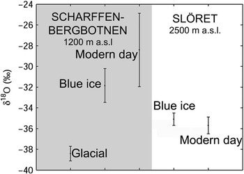
Results from the isotopic analysis of two BIAs in Dronning Maud Land are shown in Fig. 5. Scharffenbergbotnen is a closed BIA (Grinsted et al. Reference Grinsted, Moore, Spikes and Sinisalo2003), and it represents type I BIA in the classification of BIAs by Takahashi et al. (Reference Takahashi, Endoh, Azuma and Meshida1992) as mentioned earlier. “Slöret” is an open BIA of type III located at the edge of the Antarctic plateau at about 2300 m a.s.l. where the ice sheet flows over the Kirwanveggen mountain range. Isotopic analysis (Fig. 5) indicates that the major part of the surface ice of these two mountainous BIAs are of Holocene origin. This method can only be used to make the division between samples of glacial and interglacial origin, and additional information about the past changes in ice flow and surface elevation are required for correct interpretation.
The δ18O values from the Scharffenbergbotnen valley (left) and “Slöret” (right). The modern day values are measured from snow/firn samples collected in the accumulation areas of the BIAs. The values for blue ice are calculated averages from many shallow cores scattered over the BIAs. Glacial ice was only found in Scharffenbergbotnen showing clearly lower δ18O values than the modern day samples (Sinisalo et al. Reference Sinisalo, Grinsted, Moore, Meijer, Martma and van De Wal2007). See Fig. 6 for its location.

Geomorphology
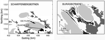
Supraglacial moraine structures can provide useful information about the age of a BIA. Hättestrand & Johansen (Reference Hättestrand and Johansen2005) studied moraines in Scharffenbergbotnen and Buråsbotnen BIAs in Dronning Maud Land (Fig. 6, see Fig. 1 for the location). Supraglacial moraines were deposited in Scharffenbergbotnen BIA during the LGM. Hättestrand & Johansen (Reference Hättestrand and Johansen2005) concluded that the survival of these moraines indicates that there was a local ablation centre and probably a BIA in the Scharffenbergbotnen valley at LGM, and it has been continuously maintained since then. Moraines on the slopes of surrounding nunataks suggest that the surface elevation of the BIA was higher during LGM than at present, and striae and gouges in the outcropping bedrock indicate past ice flow directions (Hättestrand & Johansen Reference Hättestrand and Johansen2005). Moraines drawn out from the Buråsbotnen cirque (Fig. 6), on the other hand, were deposited in the inner part of the cirque in an earlier phase, but subsequent increased accumulation in the area has caused them to be pushed and drawn out in the overall ice flow direction towards the north-west (Hättestrand & Johansen Reference Hättestrand and Johansen2005). Similarly, old supraglacial moraines and ice flow indicators in the bedrock in other BIAs can be used for reconstructing the former ice flow, and existence, surface elevation, and extent of the BIA.
Supraglacial moraines (black) and nunataks (dark grey) around BIAs (light grey) in Scharffenbergbotnen (left) and around Buråsbotnen, Milorgfjella (modified from Hättestrand & Johansen Reference Hättestrand and Johansen2005). See Fig. 1 for locations of the BIAs. The moraines form closed loops in the valley of Scharffenbergbotnen whereas they are drawn out from the cirque in Buråsbotnen.

More intensive methods
Ice flow modelling
In contrast with the methods outlined earlier, ice flow modelling produces a continuous set of ages over a BIA, or at least along selected flow lines on a BIA. A full three dimensional model is always desirable but necessary field data are often unavailable, or derived from short period observations. For example, it is often challenging to collect the appropriate ice flow velocity data on BIAs for model tuning or validation as typical velocities are only 10 cm a-1 in both horizontal and vertical components. Thus, it is much more practical to use a flow line approach than a three dimensional model, as sparse field data can be more easily incorporated into such a model.
The first modelling efforts on BIAs were made to explain meteorite findings on the surface of BIAs. Naruse & Hashimoto (Reference Naruse and Hashimoto1982) made a simple flow model to date a BIA upstream of a nunatak in Yamato Mountains based on the continuity equation (Nye Reference Nye1963). Whillans & Cassidy (Reference Whillans and Cassidy1983) produced a very simple model for the Allan Hills BIA, and a much more sophisticated approach was used by Azuma et al. (Reference Azuma, Nakawo, Higashi and Nishio1985) for the flow on South Yamato BIA in an area near a nunatak called Massif A. Azuma et al. (Reference Azuma, Nakawo, Higashi and Nishio1985) used a 30 m ice core taken 2 km upstream of the nunatak to estimate parameters for the flow law of the ice, and then computed flow lines for the ice near the nunatak, parameterizing the flow divergence near the nunatak. In common with these earlier modelling efforts, Van Roijen (Reference Van Roijen1996) parameterized ice thickness but used some limited velocity observations and 14C ages to constrain flow.
Grinsted et al. (Reference Grinsted, Moore, Spikes and Sinisalo2003) developed a volume conserving flow line model which assumes constant ice sheet geometry over time, i.e. steady state flow. The model uses field data for surface velocities, mass balance and ice thickness along a flow line, with parameterized variation of ice rheology with depth to produce particle trajectories and isochrones. This model has been applied to Scharffenbergbotnen (Grinsted et al. Reference Grinsted, Moore, Spikes and Sinisalo2003, Sinisalo et al. Reference Sinisalo, Grinsted and Moore2004, Reference Sinisalo, Grinsted, Moore, Meijer, Martma and van De Wal2007), Allan Hills (Grinsted et al. Reference Grinsted, Moore, Spikes and Sinisalo2003) and to South Yamato BIAs (Moore et al. Reference Moore, Nishio, Fujita, Narita, Pasteur, Grinsted, Sinisalo and Maeno2006).
A limitation of modelling to date is that it is prognostic only, assuming steady ice geometry. Over glacial-interglacial cycles ice sheet elevation changes must have played a significant role in ice flow at most BIAs. Additionally, it is still unclear how much of the bed of BIAs are frozen. The melting condition at the bed is essential for modelling the evolution of BIAs.
We have experimented with a three-dimensional fully coupled thermomechanical finite element model (ELMER-ICE) of Scharffenbergbotnen. Input to these models requires the geometry of glacier upper and lower boundaries and the mass and energy and fluxes across each boundary. These data are now reasonably well known for Scharffenbergbotnen, but to our knowledge is lacking for other BIAs. Output from such models includes basal temperatures (with an assumed geothermal heat flux). Results show encouraging prognostic behaviour that matches the well measured ice velocity patterns. Development of time evolving model is in progress.
Radar isochrones
Geometry is most easily found by radar sounding the BIA. Radar data can also include internal layering of the snow/blue ice transition zone (Sinisalo et al. Reference Sinisalo, Grinsted and Moore2004), which can give valuable information on accumulation rates. Isochrone dip angles can be used to validate flow model predictions. In some BIAs the dip angle has been measured directly. For example, the observed dip angle of the blue ice relative to the surrounding firn is only a few degrees on South Yamato BIA (Yokoyama Reference Yokoyama1976) while the dip angles of tephra bands in Mount Moulton are typically about 45° (Dunbar et al. Reference Dunbar, Mcintosh and Esser2008). Relatively low dip angles are found in open type BIAs while higher angles are found in closed BIAs.
The dip angle of an isochrone can be calculated from the along-flow surface velocity profile u and the ablation and accumulation gradients b′ and a′ by considering the layer geometry of the along-flow surface-age (dτ/dx) and vertical age (dτ/dz) gradients (Sinisalo et al. Reference Sinisalo, Grinsted and Moore2004). Moore et al. (Reference Moore, Nishio, Fujita, Narita, Pasteur, Grinsted, Sinisalo and Maeno2006) showed that this angle was also simply related to the accumulation rate a along the flow line, if the amount of strain thinning along the flow line can be estimated such that a at the source region is thinned to λ due to flow. These then yield

for the dip angle  .
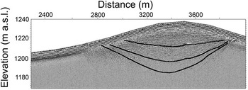
Equation (1) assumes that the ablation rate is constant over time. The two right hand side equalities of the equation are useful in different circumstances. The linear dependence of the dip angle on the horizontal distance x from the equilibrium line is useful near the equilibrium line, where radar data often show isochrones well and where strain thinning of the layers can be neglected. Dependence on x predicted from Eq. (1) is consistent with the GPR data that show near surface layers less steep than the deeper layers (Fig. 7). The strain thinning relationship in the rightmost equality is useful far from the equilibrium line where dip angles are occasionally available, such as from tephra layers. However, these functions need not to be constant over time and detailed analysis of radar profiles such as in Fig. 7 together with flow modelling should enable details of the ice accumulation pattern in the region to be well constrained.
A GPR section over a snow ridge between two BIAs in Scharffenbergbotnen valley showing dip angles of isochrones at the firn/blue ice transition zone (see Fig. 1 for location). The main closed type of BIA is on the left side of the snow ridge, and the smaller open type of BIA on the right side. Ice flows from right to left in the figure. Note that the data are not migrated, i.e. the dip angles of the layers appear steeper than they actually are. (Sinisalo et al. Reference Sinisalo, Grinsted and Moore2004)

Equation (1) shows that for an open BIA (e.g. South Yamato) flow, where u remains relatively large across the BIA, the dip angle will be low. One relevant implication of shallow dip angles is that although the ice is ancient at the surface, a horizontal ice core is not a particularly efficient way of recovering ice spanning a great age. This can also be appreciated from the roughly 50 km along flow extent of the BIA that spans about 150 kyr compared with 150 kyr spanned by the upper 1.8 km of the Dome Fuji ice core (Watanabe et al. Reference Watanabe, Jouzel, Johnsen, Parrenin, Shoji and Yoshida2003b).
Stratigraphical matching
A traditional method of dating stratigraphical records such as palaeoclimate proxies is by matching them with an established well-dated record. This requires that the proxies being compared are responding to the same climate variability, and not responding to some local variability that is unrepresented in the reference profile. The most useful stratigraphical palaeoclimate proxies appear to be relative concentration and isotopic composition of the gases trapped in the ice. However, there are problems in collecting samples suitable for gas analysis from BIAs, most likely due exchange of gases in the upper metres of the blue ice, which experiences cracking as it approaches the surface. Work on bubble expansion from a 100 m core from South Yamato BIA (Nakawo et al. Reference Nakawo, Nagoshi and Mae1988) suggests that significant release of stress occurs even at 50 m depth, though no cracks were seen below 7 m depth. Relatively small upward velocities in BIAs of order 10 cm a-1 mean that ice is in the upper 10 m of the BIA for century periods of time.
Stratigraphical matching may also be unreliable due to compositional changes as the ice sits in a near surface environment. The rate at which the ice approaches the surface is comparable with the firnification rates on the Antarctic plateau, where post-depositional changes can occur (Legrand & Mayewski Reference Legrand and Mayewski1997). This also leads to the problems in 14C dating of near surface air bubbles ice caused by in situ 14C production by cosmic-ray muons (van der Kemp et al. Reference Van der Kemp, Alderliesten, van der Borg, de Jong, Lamers, Oerlemans, Thomassen and van de Wal2002). The presence of cryoconite and biological activity in the ice can also lead to chemical conversion of species within the upper decimetre or so of ice. This can be avoided by sampling deep enough, but that leads to practical difficulties. The chemical species that appears to be most affected by near-surface processes is MSA. In profiles of 10 m cores in BIA we find no clear sign of any trend with any other species (unpublished data).
Volcanic signatures are potentially a useful method of cross-matching records extracted from BIAs and deep ice cores. However, the individual analysis of tephra by electron microscopy methods is a demanding and laborious method (e.g. Palais et al. Reference Palais, Germani and Zielinski1992, Kekonen et al. Reference Kekonen, Moore, Perämäki and Martma2005), and it is not suitable for continuous profiling at present. Proxy methods of identifying volcanic signatures from sulphate profiles (Zielinski Reference Zielinski1995), or from their electrical conductivity signature (Hammer et al. Reference Hammer, Clausen and Dansgaard1980) are problematic as the volcanic fallout is never uniform across the ice sheet, and there are significant volcanic acid fallout events rather frequently (Robock & Free Reference Robock and Free1995). This leads to difficulties in finding a unique match of a series of spikes in a BIA record with a reference ice core (Moore et al. Reference Moore, Nishio, Fujita, Narita, Pasteur, Grinsted, Sinisalo and Maeno2006).
The process of wiggle-matching using ice parameters such as stable water isotope, or major soluble ions between a BIA record and a deep ice core is perhaps more reliable, though potentially undermines the point of extracting the BIA record. The advantage of the BIA record is that it is from a different geographic area than the deep ice cores, hence we would expect to find differences in the climatic signatures between the two records. Forcing the main variability to match between deep cores sites and BIAs reduces the chances of seeing genuine climatic variability recorded in the two records.
Layer counting
A plausible direct method of dating is by counting cycles in measured parameters. This is potentially highly useful on BIAs where the annual layer thickness is greater than found deep in traditional ice cores, both because annual accumulation rates nearer the coast are higher than inland, and because the amount of strain thinning experienced is often less. Therefore the number of samples per cycle is much less limited by sample size than in vertical deep cores. The annual layer thickness at mid-Holocene measured from a single 60 cm sample at the surface of the Scharffenbergbotnen BIA, for example, is about 20 cm of ice that corresponds to 160 mm w.e., and to a horizontal age gradient of about 5.4 a m-1 (Sinisalo et al. Reference Sinisalo, Grinsted, Moore, Meijer, Martma and van De Wal2007).
BIA records from coastal areas may have less well-defined annual cycles than seen in more inland records, however, especially in those from largely sea-salt derived species (Legrand & Mayewski Reference Legrand and Mayewski1997). As with cycle counting in vertical cores, the greater the number of different annually-varying parameters that are considered, the more accurate will be the annual cycle count (Taylor et al. Reference Taylor, Alley, Meese, Spencer, Brook, Dunbar, Finkel, Gow, Kurbatov, Lamorey, Mayewski, Meyerson, Nishiizumi and Zielinski2004).
Specific difficulties with BIA layer counting are firstly the dip angle of layers. If the dip angle is too shallow it is quite possible that the small-scale topography of the ice surface will re-sample the same layer more than once along the transect. The second problem is the need for an absolute date to anchor the cycle count. Thus, it is possible that a rather accurate number of cycles could be found in a given part of the BIA, but actual age of the ice remains only known to the limits of radiometric or ice flow precision. There are practical difficulties in determining the equilibrium line, and hence zero age of the BIA. The equilibrium line will be some distance up flow from the firn line, and the upstream part of the surface ice zone is marked with old snow and firn patches that make surface sampling virtually impossible. One possible method for some BIA would be high frequency radar to count layers in the equilibrium area and firn areas until continuous surface sampling of ice could begin.
Blue ice cores
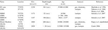
Very few blue ice cores have been studied for palaeoclimatic purposes to date (Table I). Only two horizontal ice cores have been analysed for palaeoclimate records: a 101 m long ice transect from the surface of the Scharffenbergbotnen BIA (Sinisalo et al. Reference Sinisalo, Grinsted, Moore, Meijer, Martma and van De Wal2007), and a 600 m long transect from Mount Moulton (Popp et al. unpublished). The transect in Scharffenbergbotnen was estimated to represent a 500 year mid-Holocene period. The Mount Moulton core does not include the Holocene period since that part of the BIA was covered by snow when sampling was done.
Details of Antarctic blue ice samples. The sampling sites are indicated in Fig. 1 with the codes given in the first column under the name of the core.

*Age in the middle of the 100 m blue ice core (Sigl & Schwikowski, personal communication 2009). The age span of SBB01H is estimated to be about 500 years (Sinisalo et al. Reference Sinisalo, Grinsted, Moore, Meijer, Martma and van De Wal2007).
The temporal resolution of palaeoclimate records extracted from blue ice cores vary greatly. Isotopic analysis of a sample from the horizontal transect in Scharffenbergbotnen suggested a horizontal age gradient of about 5 a m-1 corresponding to about 160 mm w.e. in mid-Holocene (Sinisalo et al. Reference Sinisalo, Grinsted, Moore, Meijer, Martma and van De Wal2007). This is equal to an annual layer thickness of about 20 cm of ice, which is greater than the layer thickness for the same age ice in traditional ice cores from high accumulation areas in coastal Antarctica such as Law Dome (Morgan et al. Reference Morgan, Wookey, Li, van Ommen, Skinner and Fitzpatrick1997). The gradient is fairly linear along the flowline over the Scharffenbergbotnen BIA, and it covers the entire Holocene period (Fig. 8). The stable isotope record from the transect in Mount Moulton, on the other hand, spans about 150 000 years within 600 m. It is the first such record of the last interglacial in West Antarctica, and shares many features with the records from deep ice cores from Vostok and EPICA-Dome C in East Antarctica (Popp et al. unpublished). Popp et al. (unpublished) found also that the trapped gases in the blue ice samples correlated well with those of Vostok ice core.
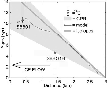
Surface age relationship along the flow line of Scharffenbergbotnen. Horizontal age gradient from high resolution isotopic analysis of a 101 m long horizontal ice core (Sinisalo et al. Reference Sinisalo, Grinsted, Moore, Meijer, Martma and van De Wal2007; grey line), and by dating of internal radar reflection horizons close to the current blue ice/snow transition zone along the flow line (Fig. 7, Sinisalo et al. Reference Sinisalo, Grinsted and Moore2004; light grey). The model output was obtained with a linearly changing temporal and spatial surface velocity and accumulation rate reaching the present values in 11 000 years. The model was adjusted to match with the 14C age of a vertical blue ice core (Sinisalo et al. Reference Sinisalo, Grinsted, Moore, Meijer, Martma and van De Wal2007). The error bars for a vertical blue ice core SBB01 are calculated using a radiocarbon calibration curve by Reimer et al. (Reference Reimer, Baillie, Bard, Bayliss, Beck, Bertrand, Blackwell, Buck, Burr, Cutler, Damon, Edwards, Fairbanks, Friedrich, Guilderson, Hogg, Hughen, Kromer, McCormac, Manning, Ramsey, Reimer, Remmele, Southon, Stuiver, Talamo, Taylor, van der Plicht and Weyhenmeyer2004). The middle part of the SBB01 H was very recently 14C dated to 4426 ± 215 years bp (Michael Sigl, Margit Schwikowski, Paul Scherrer Institut, personal communication 2009). The horizontal distance is measured starting from the bottom of the valley. The SBB01 (Table I) is located at x = 400 m and the SBB01 H at x = 1400 m.

Vertical blue ice cores of 30–101 m have been drilled for palaeoclimate studies in Mount Moulton, Scharffenbergbotnen and Yamato mountains. The age of the upper part of the vertical blue ice core drilled in Scharffenbergbotnen is about 11 kyr defined by 14C gas dating (Van der Kemp et al. Reference Van der Kemp, Alderliesten, van der Borg, de Jong, Lamers, Oerlemans, Thomassen and van de Wal2002). The 30 m blue ice core from Mount Moulton includes a gas record spanning 117 to 135 kyr (Custer Reference Custer2006) whereas the 101 m vertical blue ice core from South Yamato BIA contains a section spanning 55 to 61 kyr bp (Moore et al. Reference Moore, Nishio, Fujita, Narita, Pasteur, Grinsted, Sinisalo and Maeno2006). The Yamato Mountain blue ice core was dated by using a flowline model and the great wealth of previously unpublished and published data on South Yamato BIA that were used as inputs and constraints in a flow line model (Moore et al. Reference Moore, Nishio, Fujita, Narita, Pasteur, Grinsted, Sinisalo and Maeno2006). Geophysical data (Takahashi et al. Reference Takahashi, Ageta, Fujii and Watanabe1994, Lythe et al. Reference Lythe and Vaughan2001) allowed construction of a flow line from the ice core on the BIA to the deep borehole at Dome Fuji. In order to determine the age span, the gas data measured from the 101 m blue ice core (Machida et al. Reference Machida, Nakazawa, Narita, Fujii, Aoki and Watanabe1996) were fitted with records from Dome Fuji and other ice cores in both polar regions (Blunier & Brook Reference Blunier and Brook2001, Watanabe et al. Reference Watanabe, Kamiyama, Motoyama, Fujii, Igarashi, Furukawa, Goto-Azuma, Saito, Kanamori, Kanamori, Yoshida and Uemura2003a, Kawamura et al. Reference Kawamura, Nakazawa, Aoki, Sugawara, Fujii and Watanabe2003, Sowers et al. Reference Sowers, Alley and Jubenville2003). More precise dating was achieved with high-resolution records of electrical stratigraphy from Dome Fuji ice core. This approach of combination of methods can be used quite generally to link deep ice cores to surface outcrops on blue ice fields.
Recommendation for blue ice dating
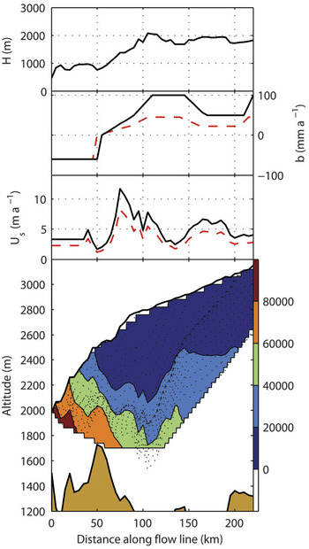
Greatest confidence in dating blue ice comes by combining many dating methods together. Generally, this means tuning flow models with other methods (Fig. 8). First, a flow model can be used to gain an initial expectation of a plausible surface age distribution, vertical age span, and the source region of the ice. Other dating methods, such as radiocarbon dating, meteorite terrestrial ages, or tephra layer dating can be used with the model in an iterative way to estimate the age distribution in a BIA. Flow modelling combined with other methods can also provide surface age distribution along the flow line, temporal changes in the size of the BIA, and ice flow velocities, and constrain elevation changes and accumulation patterns over the accumulation region (Fig. 9).
Ice thickness H, mass balance b and surface velocity Us along the SY flow line. The extent of the BIA can be seen from the region of negative b. Bottom: Modelled (Moore et al. Reference Moore, Nishio, Fujita, Narita, Pasteur, Grinsted, Sinisalo and Maeno2006, Grinsted et al. Reference Grinsted, Moore, Spikes and Sinisalo2003) particle paths (dotted lines) and isochrones (colour contours). The SY core is at 18 km along the flow line. The glacial values of b and Us were optimized by simple scaling to try to match the 60 kyr age of the SY core. Glacial accumulation (b) set to 45% of present day values in accumulation areas (dashed curve), a 5 km reduction in the BIA glacial extent, and glacial flow velocities (Us) set to 70% of present day values with a delay of 5 kyr between climate shift and ice sheet response, (dashed curves). Figure from Moore et al. Reference Moore, Nishio, Fujita, Narita, Pasteur, Grinsted, Sinisalo and Maeno2006 reproduced with the kind permission of AGU.

General remarks on blue ice areas
It is clear from investigations to date that BIAs in different parts of Antarctica have very different histories. The area covered by blue ice, the number of individual BIAs, and their geographical distribution vary mainly on an ice sheet thinning-thickening timescale. Many BIAs in Dronning Maud Land formed during the Holocene, while the South Yamato BIA seems to be stable, having been only about 10% smaller in the glacial than at present (Moore et al. Reference Moore, Nishio, Fujita, Narita, Pasteur, Grinsted, Sinisalo and Maeno2006). Large parts of central East Antarctica may have been ablation zones during the last glacial (Siegert et al. Reference Siegert, Hindmarsh and Hamilton2003), consistent with general lowing of accumulation and higher wind speeds during colder climate periods. Isolated BIAs, such as Mount Moulton, at high elevation adjacent to a nunatak only about 10 m higher than present ice cap, are likely to respond to more localized climate than the BIAs in the mountains fringing East Antarctica. In general, the BIAs accompanying the highest and steepest nunataks are most likely to be stable (Bintanja Reference Bintanja1999).
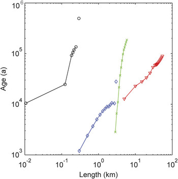
BIAs may have very different physical characteristics and temporal resolution of the palaeoclimate records extracted from blue ice cores vary greatly. Figure 10 illustrates the variability in the surface age distributions, and lengths of some BIAs along their flow lines. The large South Yamato field is associated with long flow lines (typically hundreds of kilometres), while Allan Hills and many Dronning Maud Land BIAs collect ice from only a few kilometres distance. Measured surface velocities vary from a few centimetres (e.g. Dunbar et al. Reference Dunbar, Mcintosh and Esser2008) per year to several metres per year (e.g. Moore et al. Reference Moore, Nishio, Fujita, Narita, Pasteur, Grinsted, Sinisalo and Maeno2006). As a result, the surface age gradients of BIAs can be of different magnitudes.
Comparisons of surface age distributions of four BIAs (see Fig. 1 for the locations). Ages for the ice in the Allan Hills Near Western Ice Field (green), Yamato Mountain (red) and Scharffenbergbotnen (blue) were obtained applying a flow model by Grinsted et al. (Reference Grinsted, Moore, Spikes and Sinisalo2003) except the oldest ice (28 000 years) in Scharffenbergbotnen that was originally dated by 14C dating (Van Roijen Reference Van Roijen1996). The oldest sample was not found along the main flow line, and its location along the x axis is arbitrary. The snow/blue ice transition is located at 0 at the x axis for the modelled ages. The Mount Moulton data (black) were obtained by dating of tephra bands perpendicular to the ice flow (Wilch et al. Reference Wilch, Mcintosh and Dunbar1999, Dunbar et al. Reference Dunbar, Mcintosh and Esser2008), and it is plotted on x axis so that 0 corresponds to the start of a blue ice transect (Popp et al. unpublished). The modelled ages are constrained by meteorite terrestrial ages, comprehensive datasets of geophysical and chemical parameters, and radiocarbon ages (for more details see Grinsted et al. Reference Grinsted, Moore, Spikes and Sinisalo2003, Moore et al. Reference Moore, Nishio, Fujita, Narita, Pasteur, Grinsted, Sinisalo and Maeno2006, Sinisalo et al. Reference Sinisalo, Grinsted, Moore, Meijer, Martma and van De Wal2007).

Summary and suggestions for future studies
Blue ice areas show potential for palaeoclimate research applications but very little palaeoclimate data from BIAs have been published to date. Blue ice samples collected from BIA surface may provide palaeoclimate data with higher resolution than traditional deep ice cores. In addition, many BIAs are located in areas where no deep ice cores are available. Dating of BIAs remains challenging, but as the examples in this paper show, substantial progress has been made in that field. Blue ice cores and ice flow modelling combined with other dating methods have provided insight in the variability of dynamics and sizes of the BIAs, and the surrounding ice sheet, and local climatic conditions. The conditions that create and maintain BIAs are of wide significance as they are related to the general ice sheet elevation, accumulation patterns and climate.
An opportunity offered by BIAs over traditional ice core drilling is the possibility to access to large sample volumes of old ice. Large blue ice samples are particularly useful for measurements involving trapped gases and gas isotopes. In traditional ice cores, limited number and size of ice samples across interesting climate transitions can limit the science at a particular drilling location. BIAs may also be able to provide unique data as a cross dating tool in areas where climatic or gas transitions are recorded in the BIA, and where datable tephra layers or 14C sequences are also found. BIAs in areas close to Southern Ocean may provide high resolution climatic information about the role of the Southern Ocean at last glacial transition.
Many mountain BIAs are likely situated in the area of the cold/warm transition at the bed. The bed conditions of BIAs should be studied more intensively as it is essential for modelling the evolution of BIAs.
Satellite and aerial photographic image analyses of BIAs can provide new information about the dynamics of the Antarctic ice sheet. Correlation of individual, dated tephra layers, or sets of layers, in BIAs will allow a better understanding of the geometry of the ice flow. The palaeoclimate record obtained from surface blue ice samples can be extended over wide geographical areas, though at low resolution by identifying and dating visible horizons on BIAs using the stratigraphical records from ice cores and tracking them in satellite images.
Satellite imagery shows potential to be a valuable tool in monitoring the possible areal changes in individual BIAs, and in the total extent of Antarctic BIAs. Although the overall changes in the BIA extent seem to be slow, BIAs should be monitored, especially using radar images which may allow near surface blue ice to be observed under snow cover.
Acknowledgements
We would like to thank C. Hulbe, A. Grinsted and two anonymous reviewers for comments that helped us to improve the manuscript. Finnish Antarctic Research Program (FINNARP 1999–2000, 2000–01, and 2003–04) provided the logistics for the field work. In addition, many Antarctic teams provided logistical support and data collection, especially, SANAE 39 and 40, and JARE 24 and 27. This work was primarily funded by the Academy of Finland and the Thule Institute. Parts of this work were funded by the Arctic graduate school ARKTIS, and by grants from the Faculty of Natural Sciences, Oulu University and the University Pharmacy Foundation (Oulu). Figure 9 is reproduced with the kind permission of AGU.