2 The population balance equation

The PBE governs the evolution of the droplet number density function, $n$ , in a phase space, $R$ . The latter is decomposed into the coordinate space, $\boldsymbol{x}=(x_{1},x_{2},x_{3})$ , and the property (or state) space, $\unicode[STIX]{x1D743}=(\unicode[STIX]{x1D709}_{1},\ldots ,\unicode[STIX]{x1D709}_{M})$ , which can include droplet size (commonly, volume), shape, surface area, morphology, etc. Hence, $n(\unicode[STIX]{x1D743};\boldsymbol{x},t)\,\text{d}\boldsymbol{x}\,\text{d}\unicode[STIX]{x1D743}$ is defined as the ensemble of entities having coordinates in the range $(\text{d}\boldsymbol{x}\text{d}\unicode[STIX]{x1D743})$ around $(\boldsymbol{x},\unicode[STIX]{x1D743})$ at a given time, t. Using this definition, the PBE is written as (Sporleder et al. Reference Sporleder, Borka, Solsvik and Jakobsen2012)

(2.1) $$\begin{eqnarray}\frac{\unicode[STIX]{x2202}n}{\unicode[STIX]{x2202}t}+\unicode[STIX]{x1D735}_{\boldsymbol{x}}(\boldsymbol{u}n)+\unicode[STIX]{x1D735}_{\unicode[STIX]{x1D743}}(\dot{\unicode[STIX]{x1D743}}n)=w,\end{eqnarray}$$

where $\boldsymbol{u}(\unicode[STIX]{x1D743};\boldsymbol{x},t)$ and $\dot{\unicode[STIX]{x1D743}}(\unicode[STIX]{x1D743};\boldsymbol{x},t)$ are the velocities in the physical and the property spaces, respectively. In this study, which is motivated by ongoing work to simulate secondary atomisation of sprays, the property space, $\unicode[STIX]{x1D743}=(\unicode[STIX]{x1D709}_{1},\unicode[STIX]{x1D709}_{2})$ , includes volume, $\unicode[STIX]{x1D709}_{1}=V$ , and shape, $\unicode[STIX]{x1D709}_{2}=S$ , in line with the experimental observations of Kourmatzis & Masri (Reference Kourmatzis and Masri2015) briefly mentioned above. The source term, $w$ , is the net rate of change of number density due to discrete births and deaths of droplets as a result of breakages and agglomeration. It is typically a highly nonlinear function of the interactive forces between the carrier and dispersed phases. In the PDF-PBE, however, this nonlinear term appears naturally in closed form; in contrast to moment closure methods which require further modelling of source terms. The third term on the left-hand side of equation (2.1) accounts for growth and shrinkage due to condensation and evaporation leading to changes in droplet size and/or shape. It is neglected here due to those phenomena having a relatively small impact compared to breakages in the secondary atomisation region.

Equation (2.1) holds in either laminar or turbulent flows although for the latter, a numerical method to solve it directly needs to resolve all the scales of turbulence. Therefore, for practically relevant droplet simulations, some form of averaging or statistical emulation of the turbulent field is required. We adopt here a hybrid approach where LES is employed for the carrier phase and a PDF version of the PBE is chosen for the dispersed phase. The former is conventional and is solved in an Eulerian fashion on a finite volume grid. The latter is a continuous function but its turbulent distribution is represented discretely and stochastically by an ensemble of Lagrangian notional particles in a Monte Carlo simulation. In general, the number density function represents a range of droplet sizes and shapes with vastly different slip velocities. The different trajectories of droplets with different inertia eliminates the possibility of representing all droplet sizes and shapes on each notional particle. A key innovation in our model is to divide the PDF-PBE into classes, where each class represents the turbulent distribution of the number density function of droplets that have similar inertial interactions with the carrier gas. In the present section the model equations are presented for a single class and in the next section the selection of the classes based on a method known as Stokes binning is introduced.

The notional particles in each class evolve according to stochastic differential equations (Pope Reference Pope1985; Minier & Peirano Reference Minier and Peirano2001)

(2.2) $$\begin{eqnarray}\left.\begin{array}{@{}l@{}}\text{d}\boldsymbol{X}=\boldsymbol{U}\,\text{d}t,\\[2.0pt] \text{d}\boldsymbol{U}=\boldsymbol{A}\,\text{d}t,\\[2.0pt] \text{d}\boldsymbol{N}=\boldsymbol{W}\,\text{d}t.\end{array}\right\}\end{eqnarray}$$

Here, the upper case symbols denote values associated with notional particles, and are the sample space of the corresponding physical variables in equation (2.1). $\boldsymbol{X}$ is the notional particle position while $\boldsymbol{U}$ and $\boldsymbol{A}$ are the velocity and the acceleration, respectively. $\boldsymbol{N}$ is the number density function and $\boldsymbol{W}$ is the source term. Note that the source term appears naturally in its closed, instantaneous form and no filtering or averaging is required.

Droplet dispersion in a turbulent flow field is governed by the model for the acceleration, $\boldsymbol{A}$ , which depends on both dispersed phase and carrier flow properties. The acceleration due to the drag force is taken to be equal to the first term of the formulation given by Maxey & Riley (Reference Maxey and Riley1983) for the force per droplet mass

(2.3) $$\begin{eqnarray}\text{d}\boldsymbol{U}=\frac{1}{\langle \unicode[STIX]{x1D70F}_{p}\rangle }(\boldsymbol{v}-\boldsymbol{U})\,\text{d}t,\end{eqnarray}$$

where $\langle \unicode[STIX]{x1D70F}_{p}\rangle$ is the mean (across the class of droplets) response time due to fluid–droplet interaction forces. If each PDF-PBE class is limited to droplets of only one size and shape (the so-called brute force method) then $\langle \unicode[STIX]{x1D70F}_{p}\rangle =\unicode[STIX]{x1D70F}_{p}=\unicode[STIX]{x1D70F}_{p}(\unicode[STIX]{x1D743};x,t)$ which is modelled as discussed later in this section. A DNS of the carrier fluid can provide the instantaneous gaseous velocities, $\boldsymbol{v}$ , but only filtered velocities are available if LES is applied to the carrier fluid. In that case, $\boldsymbol{v}$ , can be decomposed into the filtered velocity, $\overline{\boldsymbol{v}}$ and the subgrid velocity, $\boldsymbol{v}^{\prime }$ . If the droplet response time is large compared to the time scales of the turbulent flow, direct effects of subgrid scales are insignificant and hence a subgrid model in the stochastic equations is not required (Wang & Squires Reference Wang and Squires1996). In cases where the droplet response time is of the same order of magnitude as the flow time scales, a model is required for the unresolved velocity. The approximate deconvolution model (ADM) (Kuerten Reference Kuerten2006) and the Langevin model (Minier & Peirano Reference Minier and Peirano2001; Pozorski & Apte Reference Pozorski and Apte2009) are widely employed to reconstruct the residual (or subgrid scale) carrier fluid velocity. The latter is employed in the present study. Following Pozorski & Apte (Reference Pozorski and Apte2009), the subgrid velocity is computed using

(2.4) $$\begin{eqnarray}\text{d}v_{i}^{\prime }=-\frac{v_{i}^{\prime }}{\unicode[STIX]{x1D70F}_{L}}\,\text{d}t+\sqrt{\frac{4K_{sgs}/3}{\unicode[STIX]{x1D70F}_{L}}}\,\text{d}\unicode[STIX]{x1D714}_{i},\end{eqnarray}$$

where $\text{d}\unicode[STIX]{x1D714}$ is an increment of the Wiener process, $K_{sgs}$ is the subgrid kinetic energy and $\unicode[STIX]{x1D70F}_{L}$ is the characteristic time scale which differs in the directions parallel, $\unicode[STIX]{x1D70F}_{L,||}$ and perpendicular, $\unicode[STIX]{x1D70F}_{L,\bot }$ to the relative velocity. They are defined as

(2.5a,b ) $$\begin{eqnarray}\unicode[STIX]{x1D70F}_{L,||}=\frac{\unicode[STIX]{x1D70F}_{sgs}}{\sqrt{1+\unicode[STIX]{x1D6FD}^{2}\unicode[STIX]{x1D701}^{2}}},\quad \unicode[STIX]{x1D70F}_{L,\bot }=\frac{\unicode[STIX]{x1D70F}_{sgs}}{\sqrt{1+4\unicode[STIX]{x1D6FD}^{2}\unicode[STIX]{x1D701}^{2}}},\end{eqnarray}$$

where $\unicode[STIX]{x1D701}$ is $|\overline{\boldsymbol{v}}-\boldsymbol{U}|/\sqrt{2K_{sgs}/3}$ , $\unicode[STIX]{x1D70F}_{sgs}$ is the time scale of subgrid fluid motions and $\unicode[STIX]{x1D6FD}$ is the ratio of Lagrangian to Eulerian time scales. $\unicode[STIX]{x1D70F}_{sgs}$ is defined as $C(\unicode[STIX]{x1D6E5}_{f}/\sqrt{2K_{sgs}/3})$ where $C$ is the model constant and $\unicode[STIX]{x1D6E5}_{f}$ is the filter size. Here, $\unicode[STIX]{x1D6FD}=1$ and $C=1$ are employed in the simulations as recommended by Pozorski & Apte (Reference Pozorski and Apte2009).

The droplet response time may be defined as

(2.6) $$\begin{eqnarray}\frac{1}{\unicode[STIX]{x1D70F}_{p}}=\frac{1}{2}C_{D}\frac{\unicode[STIX]{x1D70C}}{\unicode[STIX]{x1D70C}_{d}}\frac{A_{d}}{V_{d}}|\boldsymbol{v}-\boldsymbol{U}|,\end{eqnarray}$$

where $C_{D}$ is the drag coefficient, $\unicode[STIX]{x1D70C}$ is the carrier fluid density, $\unicode[STIX]{x1D70C}_{d}$ is the droplet density, $A_{d}$ is a reference area (usually droplet projected area) and $V_{d}$ is the droplet volume. The drag coefficient is a nonlinear function of the slip velocity, $\boldsymbol{v}-\boldsymbol{U}$ , and it depends on the droplets’ shape. Three different regimes may be defined based on the Reynolds number; Stokes drag regime ( $Re\ll 1$ ), intermediate Reynolds regime ( $1<Re<1000$ ) and Newton-drag regime ( $Re\geqslant 1000$ ). In the Newton-drag regime, $C_{D}$ is approximately independent of Reynolds number and it is reasonable to define a constant critical drag coefficient. In the Stokes-drag regime and intermediate Reynolds regime, the empirical formulation for $C_{D}$ is well known for spherical droplets but more complicated expressions are required for non-spherical shapes (Loth Reference Loth2008). The most successful approaches (Ganser Reference Ganser1993; Loth Reference Loth2008) use a combination of drag corrections for the Stokes regime and the Newton-drag regime. Hence, for non-spherical droplet shapes, the drag coefficient can be expressed as (Ganser Reference Ganser1993)

(2.7) $$\begin{eqnarray}C_{D}=C_{D}^{\ast }C_{\mathit{shape}},\end{eqnarray}$$

where $C_{\mathit{shape}}$ is a Newton-drag correction factor. $C_{D}^{\ast }$ is defined based on the formulation for the spherical droplets (Loth Reference Loth2008)

(2.8) $$\begin{eqnarray}C_{D}^{\ast }=\frac{24}{Re^{\ast }}(1+0.15{Re^{\ast }}^{2/3}),\end{eqnarray}$$

where $Re^{\ast }=C_{\mathit{shape}}Re/f_{\mathit{shape}}$ . $Re$ is defined as $\unicode[STIX]{x1D70C}|\boldsymbol{U}-\boldsymbol{v}|d_{p}/\unicode[STIX]{x1D707}$ where $d_{p}$ is the effective diameter and $\unicode[STIX]{x1D707}$ is the carrier fluid viscosity. In this study, in addition to spherical droplets, we also consider oblate spheroid droplets. By definition, $C_{\mathit{shape}}$ and $f_{\mathit{shape}}$ are equal to one for spheres whereas they are 2.1 and 1.02, respectively, for oblate spheroids (Loth Reference Loth2008). The critical drag coefficient is 0.42 for spheres and 0.84 for oblate spheroids, respectively (Loth Reference Loth2008).

3 The method of Stokes binning

The critical challenge is to ensure that a single notional particle can represent a class of the number density function without significantly compromising the accuracy of the droplets’ inertial trajectories. If the dispersed phase was not subject to inertial forces it would be possible to solve the PDF-PBE on an ensemble of notional particles where each particle in the turbulent flow represents a single realisation of the entire number density function (Rigopoulos Reference Rigopoulos2007). However, this is not possible when inertial forces are important. One approach, referred to hereon as the brute force option ensures that each notional particle represents only one size and one shape of droplets. Then, each notional particle essentially becomes a point model for a droplet. This computationally expensive brute force approach is similar to that used by Bini & Jones (Reference Bini and Jones2008) although their method was not derived from the point of view of the population balance equation.

Here we propose a more numerically efficient alternative to the brute force method. Effects of inertia may be quantified through the Stokes number defined as $St=\unicode[STIX]{x1D70F}_{p}/\unicode[STIX]{x1D70F}_{f}$ where $\unicode[STIX]{x1D70F}_{f}$ is the fluid characteristic time scale. The Stokes number expresses the response of an inertial droplet to changes in the carrier flow (e.g. due to eddies). Droplets with different sizes and shapes experience different drag forces and therefore exhibit different accelerations. For $St\ll 1$ , droplets have small inertia and quickly accelerate to the local flow velocity hence closely following the flow streamlines. For $St\gg 1$ , droplets have large inertia and are increasingly less affected by the variations in the carrier flow. We can define specific Stokes number bins (i.e. intervals) of width $\unicode[STIX]{x0394}St$ in which inertial droplets may be assumed to have approximately the same dynamic response to the carrier flow. If $dSt$ represents the range of Stokes numbers of inertial droplets represented by a notional particle then $dSt\leqslant \unicode[STIX]{x0394}St$ is the criterion by which we dynamically select the PDF-PBE classes in the simulations. It is emphasised that the Stokes number is a time-dependent variable that is updated as the slip velocity changes. The acceleration of a notional particle representing a turbulent realisation of a class of droplets is then determined by the average response time, $\langle \unicode[STIX]{x1D70F}_{p}\rangle$ , calculated over the droplets represented by that particle. Notional particles may be split during the simulation to ensure the criterion $dSt\leqslant \unicode[STIX]{x0394}St$ is met even as flow conditions change. In principle, it would also be possible to merge notional particles when two or more nearby particles fall within the same Stokes bin. While merging is not attempted in the present work, we note that care would be needed as this option would introduce errors in the form of numerical diffusion as number density would be artificially translated across a finite distance.

The specification of $\unicode[STIX]{x0394}St$ is an open question. If it is too large then the simulations may become inaccurate as droplets with very different Stokes numbers would have the same acceleration in response to variations in the carrier, and if too small the computational cost could become very large. An optimal choice of the Stokes bins can reduce the required number of notional particles leading to a significant reduction in computational cost compared to the existing brute force method while, at the same time, maintaining an acceptably high level of accuracy. Below we develop a rigorous procedure for selecting the Stokes bins for any range of droplet sizes and shapes.

Temporal evolution of the velocity of a single droplet is governed by equation (2.3) where $\langle \unicode[STIX]{x1D70F}_{p}\rangle =\unicode[STIX]{x1D70F}_{p}$ . Integration of this equation over a time interval $t$ while holding $\unicode[STIX]{x1D70F}_{p}$ and $v$ constant yields (Peirano et al. Reference Peirano, Chibbaro, Pozorski and Minier2006)

(3.1) $$\begin{eqnarray}\boldsymbol{U}(t_{0}+t)=\boldsymbol{U}(t_{0})+(\boldsymbol{U}(t_{0})-\boldsymbol{v})\left(\exp \left(-\frac{t}{\unicode[STIX]{x1D70F}_{p}}\right)-1\right).\end{eqnarray}$$

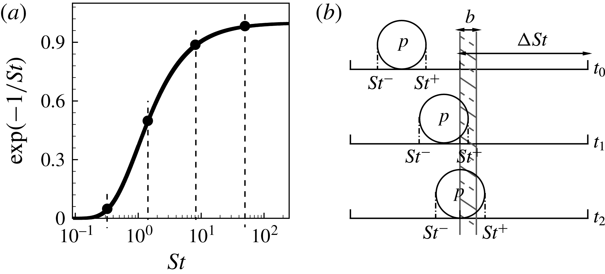
We consider $t=\unicode[STIX]{x1D70F}_{f}$ to investigate the droplet response over the carrier flow time scale. It can be seen that the change in droplet velocity is governed by an exponential function, $g=\exp (-\unicode[STIX]{x1D70F}_{f}/\unicode[STIX]{x1D70F}_{p})=\exp (-1/St)$ . Figure 1(a) shows this function which asymptotes to zero at low Stokes numbers, indicating that any slip velocity will result in a droplet immediately accelerating to match the carrier flow. We choose $St=0.25$ corresponding to $g\approx 0.02$ as a lower cutoff with droplets in the range $0<St<0.25$ deemed to be non-inertial. For large Stokes number, the function asymptotes to unity indicating that a droplet is not sensitive to a slip velocity. We choose $St=50$ corresponding to $g\approx 0.98$ as an upper cutoff with the trajectory of droplets in the range $50<St<\infty$ deemed to be marginally responsive to fluid–droplet interactions. The cutoffs are selected for convenience only and may be changed.

The interval $0.25<St<50$ exhibits strong fluid–droplet interactions and it is not obvious a priori how droplets in that range should be binned in terms of the number and width of each Stokes bin. Obviously, we want the minimum possible number of bins while maintaining accuracy. Our testing has revealed that constant spacing in logarithmic space works best with a series of numerical trials conducted and discussed in the next section to find the optimum number of equally sized bins; $\unicode[STIX]{x0394}St_{i}=\log St_{i+1}-\log St_{i}$ where $St_{i+1}$ and $St_{i}$ are the bin limits for $i$ th bin. To illustrate, figure 1(a) shows bins corresponding to $\unicode[STIX]{x0394}St=0.76$ resulting in five bins in total (including the non-inertial and non-responsive bins in the low and high Stokes limits). Since the shape of the function $g$ is case independent, it is only necessary to conduct the tests once for a range of flow types to investigate convergence of the Stokes binning method as $\unicode[STIX]{x0394}St$ decreases. The optimum value of $\unicode[STIX]{x0394}St$ is subjective to the desired accuracy and availability of computational resources. Progressively reducing $\unicode[STIX]{x0394}St$ and thus increasing the number of bins will eventually lead to each notional particle representing only a single droplet size and shape. This is the brute force method. Once the value of $\unicode[STIX]{x0394}St$ which gives the desired compromise between accuracy and cost is known, the number of Stokes bins accessed in any particular simulation is determined by the range of Stokes numbers present in the flow.

It is noted that in deriving a criteria for selecting PDF-PBE classes based on Stokes bins we have considered only the acceleration due to the drag force. Exclusion of other factors, such as gravitational force, does not diminish the generality of the Stokes binning approach as equation (2.3) can be integrated in fractional steps for each such factor.

Figure 1.

Schematic view of Stokes binning; (a) exponential function $g$ versus $St$ and (b) fuzzy Stokes boundaries.

4 Test cases studied and numerical methods

The model is validated against two sets of data. The first set consists of a series of numerical test cases of polysized and polyshaped droplets dispersed in a turbulent jet whereas the second set includes an experimental case of dispersed spherical droplets in a turbulent round jet (Kennedy & Moody Reference Kennedy and Moody1998). Although the experimental data are valuable for validation, they are not sufficient to perform a systematic analysis of different aspects of the model. Hence, the first data set is conducted to investigate the accuracy, convergence and cost of the postulated Stokes binning method in fine detail. In the numerical test cases, two types of simulations are performed; droplet simulations and notional particle simulations. The droplet simulations refer to conditions where each computational point represents an individual droplet. The notional particle simulations represent the PDF-PBE solution. The droplet simulations are taken as baseline validation data against which the notional particle simulations are compared. In the experimental test case only notional particle simulations are performed. Details of both data sets are presented below where set I and set II refer to the numerical and experimental cases, respectively.

4.1 Turbulent droplet-laden jet – set I

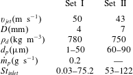
Numerical cases studied here include injection of polysized and polyshaped droplets into a turbulent jet. For this purpose, the evolution of a relatively high velocity, statistically stationary air jet at atmospheric pressure is simulated using a compressible LES code with a standard Smagorinsky subgrid model implemented in an open source C++ code known as OpenFOAM. Table 1 presents key parameters used in the simulations. The mean jet velocity, $v_{jet}$ , is taken at $50~\text{m}~\text{s}^{-1}$ whereas the coflow velocity is $1~\text{m}~\text{s}^{-1}$ . The jet diameter, $D$ , is 4 mm. The computational domain is a three-dimensional rectangular mesh of $20D$ in the axial direction and $10D$ in both transverse directions. Time-varying realistic turbulent velocity boundary conditions are applied for the inflow jet based on a turbulence intensity of 15 % and an integral length-to-jet diameter ratio of 0.125. Fixed total pressure boundary conditions are considered for the domain side and the outlet whereas zero pressure gradient is applied at the inflow. The hexahedral mesh has approximately 1 M cells uniformly distributed in all directions with a mesh size of 0.5 mm to ensure that an appropriate corresponding Eulerian filter size is applied in the shear layer (Colucci et al. Reference Colucci, Jaberi, Givi and Pope1998). The ratio between the resolved kinetic energy, $K_{res}$ , and the total kinetic energy, $K=K_{res}+K_{sgs}$ , is commonly employed to ensure the suitability of the computational meshes for LES computations. At least 80 % of the total kinetic energy should be resolved in the LES (Pope Reference Pope1985). Here, 99 % of the domain have a value of $K_{res}/K$ larger than 0.8 confirming a good mesh quality.

Table 1.

Parameters for test cases studied.

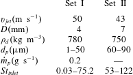
For simplicity, the effects of the inertial droplet motions on the carrier phase are not taken into account. The droplets have a uniform density of $780~\text{kg}~\text{m}^{-3}$ (typical of hydrocarbon fuels) and a mass loading is $0.2~\text{g}~\text{s}^{-1}$ . The droplets size ranges from $1~\unicode[STIX]{x03BC}\text{m}$ to $50~\unicode[STIX]{x03BC}\text{m}$ with a constant size interval of $2~\unicode[STIX]{x03BC}\text{m}$ . The range of inlet Stokes numbers, defined as $St_{inlet}=\unicode[STIX]{x1D70C}d_{p}^{2}v_{jet}/18\unicode[STIX]{x1D707}D$ , is also presented in table 1. It should be noted that, for the purposes of dynamically selecting the PDF-PBE classes and calculating the droplet or notional particle acceleration, the Stokes numbers are dynamically computed using $\unicode[STIX]{x1D70F}_{p}$ , calculated from equation (2.6), and $\unicode[STIX]{x1D70F}_{f}$ which is defined as $\unicode[STIX]{x1D6FF}/\sqrt{2K_{sgs}/3}$ where $\unicode[STIX]{x1D6FF}$ is the radial distance at half-maximum of the mean axial carrier flow velocity. The dispersion of both spherical and oblate spheroidal droplets are investigated. Two different droplet injection configurations are considered here; coflow and cross-flow. In the former case, droplets are injected into the jet with the mean jet carrier velocity whereas in the latter case, droplets are injected at right angles to the air jet with a velocity of 6.5 $\text{m}~\text{s}^{-1}$ from an injector located 1.5 mm downstream of the air nozzle exit.

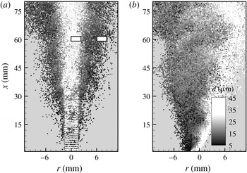
Figures 2(a) and 2(b) show droplet concentrations at 12 ms after injection for the coflow and cross-flow injector configurations, respectively. The data are from the spherical baseline droplet simulations without droplet breakage and the grey scale code indicates the droplet size. As can be seen, the heavy droplets (represented by the white colour), corresponding to high Stokes numbers, follow their own trajectories and they are simply convected downstream with only a small detectable response to fluid–droplet interactions. While light droplets (represented by the black colour) with small Stokes numbers track the flow pattern and disperse with the carrier gas from their initial injection trajectories.

Figure 2.

Instantaneous scatter plot of droplets from (a) coflow and (b) cross-flow injectors in the turbulent jet set I. The data are obtained from baseline spherical droplet simulations where each computational point represents an individual droplet. The probe locations used in the detailed analysis are denoted by the two rectangular boxes in (a).

5 Results and discussion

We first investigate convergence of the Stokes binning method by reducing $\unicode[STIX]{x0394}St$ . This is followed by studying the performance of the PDF-PBE model in reproducing the dispersion of polysized but monoshaped droplets. The PDF-PBE results are then presented for the simultaneous dispersion of polysized and polyshaped droplets. In these simulations we focus only on the dispersion so the source term, $w$ , in equation (2.2) is zero. Lastly, we test the PDF-PBE model with Stokes binning in a case involving the dispersion and breakage of spherical droplets, in which case the source term in equation (2.2) is non-zero. It should be noted § 5.2.3 demonstrates the model performance against the experiment (jet set II) while others sections present the results corresponding to the condition of the jet set I.

5.1 Stokes binning

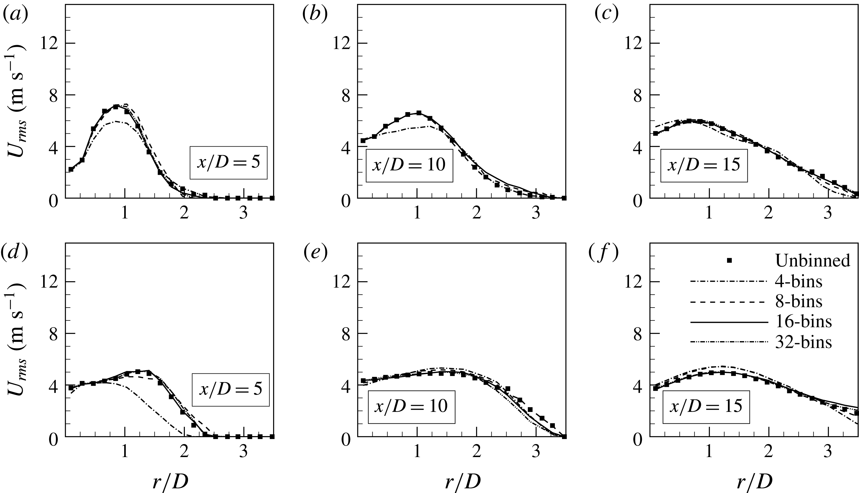
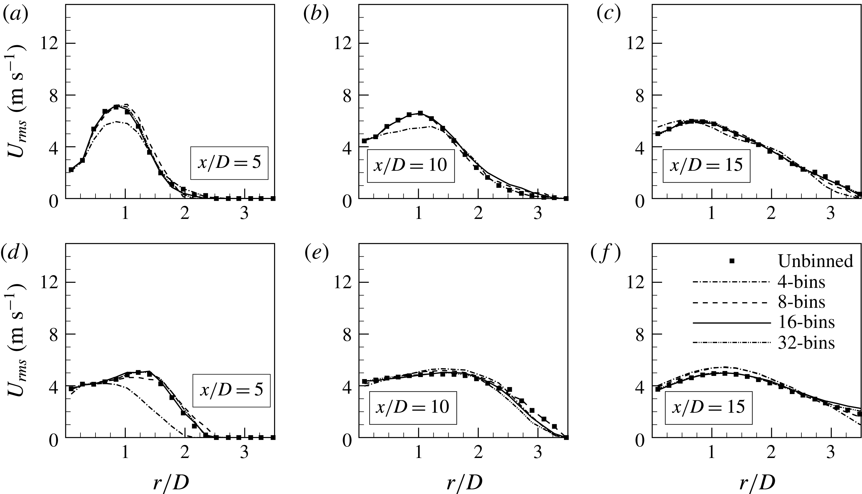
To demonstrate convergence with an increasing number of Stokes bins, we repeat the droplet simulations in the turbulent jet set I (see figures 2 a and 2 b) but this time with the inclusion of Stokes bins. These are not yet full PDF-PBE simulations with notional particles. Here, each computational point still represents a single droplet but those droplets are lumped together into Stokes bins solely for the purpose of calculating their accelerations determined from the mean droplet response time for each bin. Figure 3 presents radial profiles of the axial droplet velocity root mean square (r.m.s.), $U_{rms}$ , for the coflow (first row) and the cross-flow (second row) injector configurations at three axial locations downstream of the jet exit plane; $x/D=5$ , 10 and 15. The 4-, 8-, 16- and 32-bins cases correspond to $\unicode[STIX]{x0394}St=1.15$ , $0.38$ , $0.16$ and $0.09$ , respectively. The predicted $U_{rms}$ is sensitive to the number of bins but quickly converges to the unbinned (baseline) result. For both configurations, the results obtained using eight bins are in excellent agreement with the unbinned solution and increasing of the number of bins to 16 and then 32 only marginally changes the results. The outcomes confirm that eight bins provides sufficient accuracy for predicting $U_{rms}$ in the present flow configurations. We therefore employ eight Stokes bins as a criterion for the notional particle simulations presented in the following sections.

Figure 3.

Radial profiles of $U_{rms}$ for (a–c) the coflow and (d–f) the cross-flow injectors for the test cases set I. Results are obtained from spherical droplet simulations with Stokes binning only for the purpose of calculating droplet acceleration.

5.2 PDF-PBE simulations of polysized droplets

5.2.1 Spherical droplets

Simulations are performed using notional particles representing the PDF solution of the number density, called either notional particle or PDF-PBE simulations. The focus is first on monoshaped spherical droplets of various sizes. A set of identical notional particles is injected into the domain while the mass loading and initial droplet size distribution are the same as those in the baseline droplet simulations for the turbulent jet set I. At injection, a notional particle initially represents the entire range of droplet sizes. However, it immediately splits into as many as eight notional particles corresponding to the Stokes bin criterion established in the previous section.

As the Stokes number is a nonlinear function of the slip velocity, the range of Stokes numbers represented by a notional particle may increase or decrease depending on the local flow conditions. As discussed in § 3, a notional particle may split into two (or even more) notional particles at each time step to maintain the particle Stokes range within the bin limits. To avoid the intractable computational cost of splitting into too many notional particles, especially in the frequently encountered situation where movement across a Stokes bin boundary is only temporary, so-called fuzzy Stokes boundaries are defined. Figure 1(b) schematically illustrates the temporal evolution of a notional particle representing droplets over a range of Stokes numbers from $St^{-}$ to $St^{+}$ . The shaded area shows the fuzzy band of width $b$ at the interface between two bins of width $\unicode[STIX]{x0394}St$ . At $t=t_{0}$ , the notional particle is entirely inside the bounds of the bin on the left. At $t=t_{1}$ , the particle Stokes range is updated due to some variation in the local flow conditions and hence $St^{+}$ slightly exceeds the upper limit of the bin on the left but remains inside the fuzzy boundary. At $t=t_{2}$ , $St^{+}$ exceeds the upper limit of the fuzzy boundary and is partly inside the bin on the right. Consequently the notional particle should be split into two notional particles to satisfy the Stokes binning criterion. The opposite occurs in the case where $St^{-}$ represented by a notional particle is decreasing with time. It would only split once it goes below the lower limit of a fuzzy boundary.

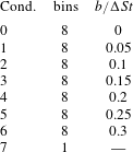
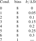
It is obvious that increasing the width of the fuzzy Stokes boundary results in lower computational cost but also lower accuracy. To find the optimal width, notional particle simulations are performed for the different boundary widths shown in table 2. The fuzzy boundary width, $b$ , is defined as a portion of the bin size, $\unicode[STIX]{x0394}St$ , with increasing width from conditions 0 through to 6. For comparison purposes, a $\text{7th}$ condition is tested whereby the Stokes binning criterion is ignored and a single notional particle can represent all droplet sizes regardless of the inertial forces on them.

Figure 4.

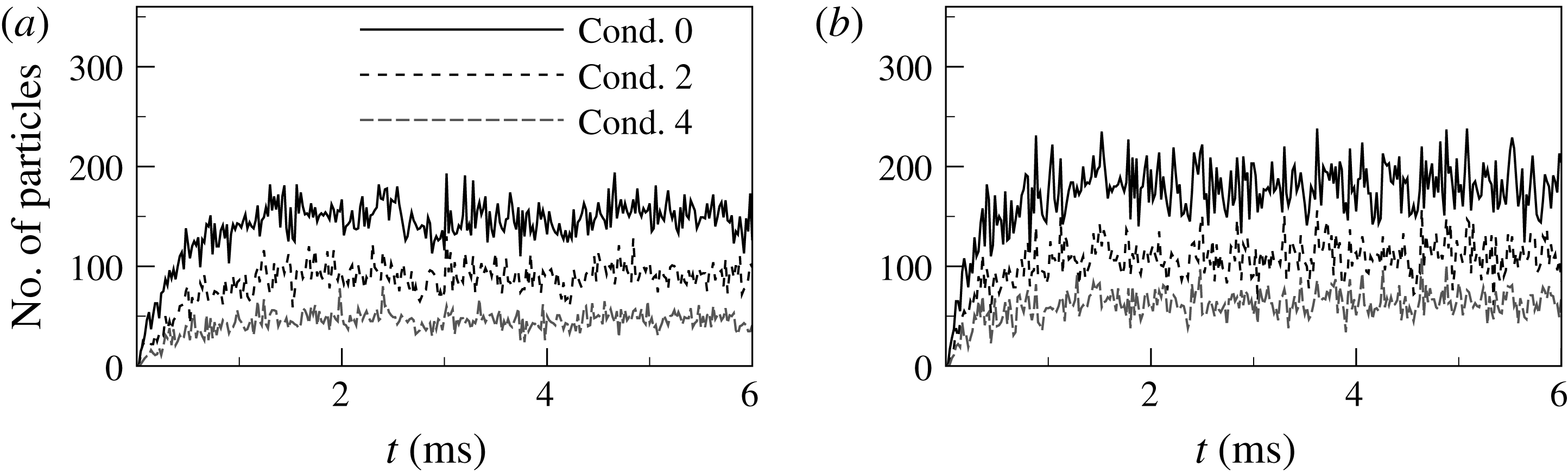
Number of split notional particles per time step for the (a) coflow and (b) cross-flow injectors. Results are for turbulent jet set I.

Figure 5.

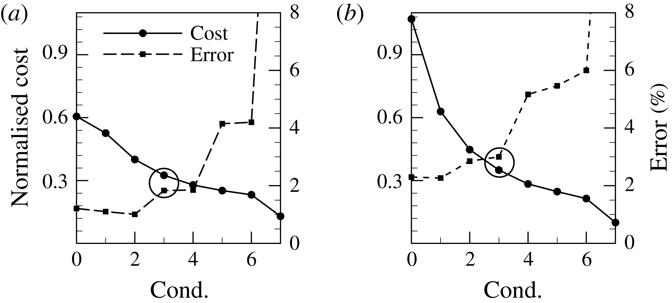
Normalised computational costs and errors for conditions defined in table 2 for the (a) coflow and (b) cross-flow injectors. Results are for turbulent jet set I.

Table 2.

Conditions considered to find the optimal fuzzy Stokes boundary width.

Figure 6.

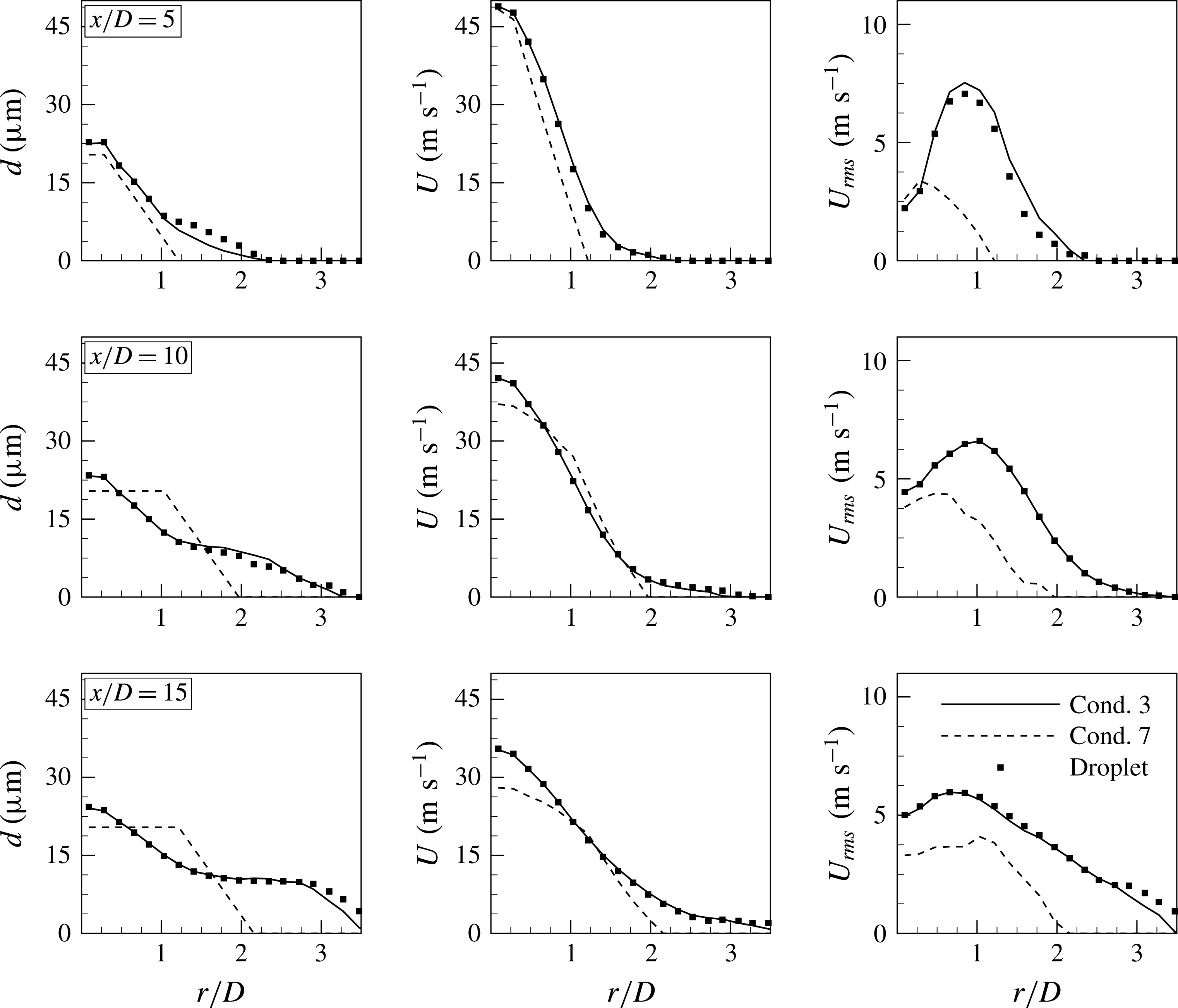
Radial profiles of the mean diameter, the mean velocity and the velocity r.m.s. at three axial locations in the coflow injector configuration with polydispersed spherical droplets – the turbulent jet set I.

Figure 4 shows the number of notional particles required to be split at each time step according to conditions 0, 2 and 4 in table 2 for both the coflow and cross-flow configurations in turbulent jet set I. The number of split particles increases quickly at early times due to the initial injection of unbinned notional particles, while it becomes statistically steady from approximately 1 ms after the start of the droplet injection. As expected, the number of split particles decreases as $b/\unicode[STIX]{x0394}St$ increases from 0 to 0.2. Figure 5 presents the computational cost and the averaged error for all conditions defined in table 2. The computational cost of notional particle simulations is normalised by the computational cost of the baseline droplet simulations. The average error is computed from the centreline values of $U_{rms}$ obtained using the notional particles in comparison with the baseline droplet simulation. The cost of the Cond. 0 simulation with eight Stokes bins but $b/\unicode[STIX]{x0394}St=0$ is already only 60 % of the cost of the baseline droplet simulations and that computational cost decreases further as the fuzzy boundary width is increased. The opposite is true for the error, increasing (slowly at first) from a minimum value of approximately 2 % in Cond. 0 to Cond. 6 values of approximately 4 % in the coflow configuration and 6 % in the cross-flow configuration. The computational cost is, of course, minimum for Cond. 7 in both configurations since the number of split particles is zero, however, the error is significantly higher than other conditions (more than 20 %). In the following, results are presented for Cond. 3 which in our view provides a pragmatic compromise between computational cost and error for both flow configurations.

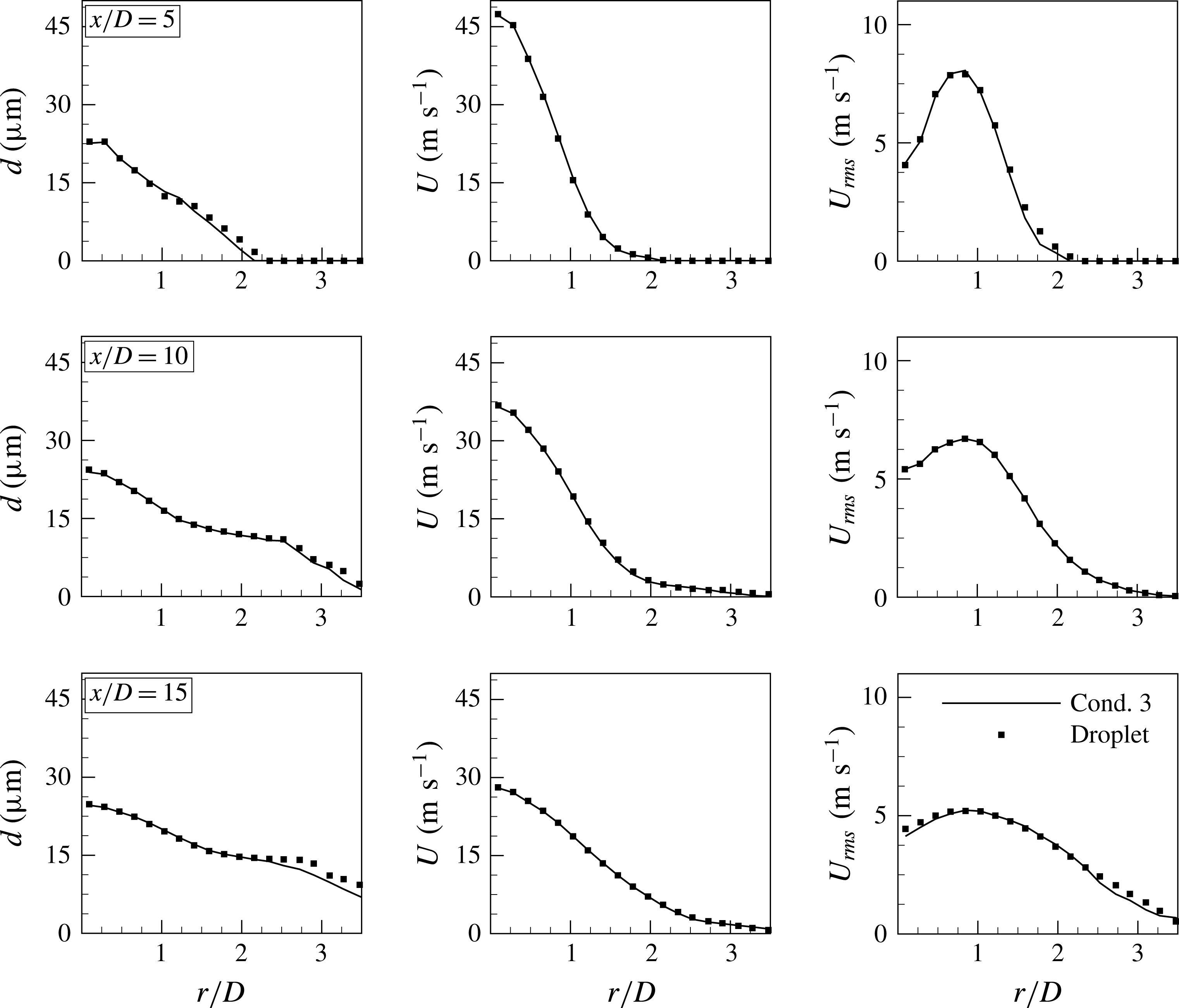
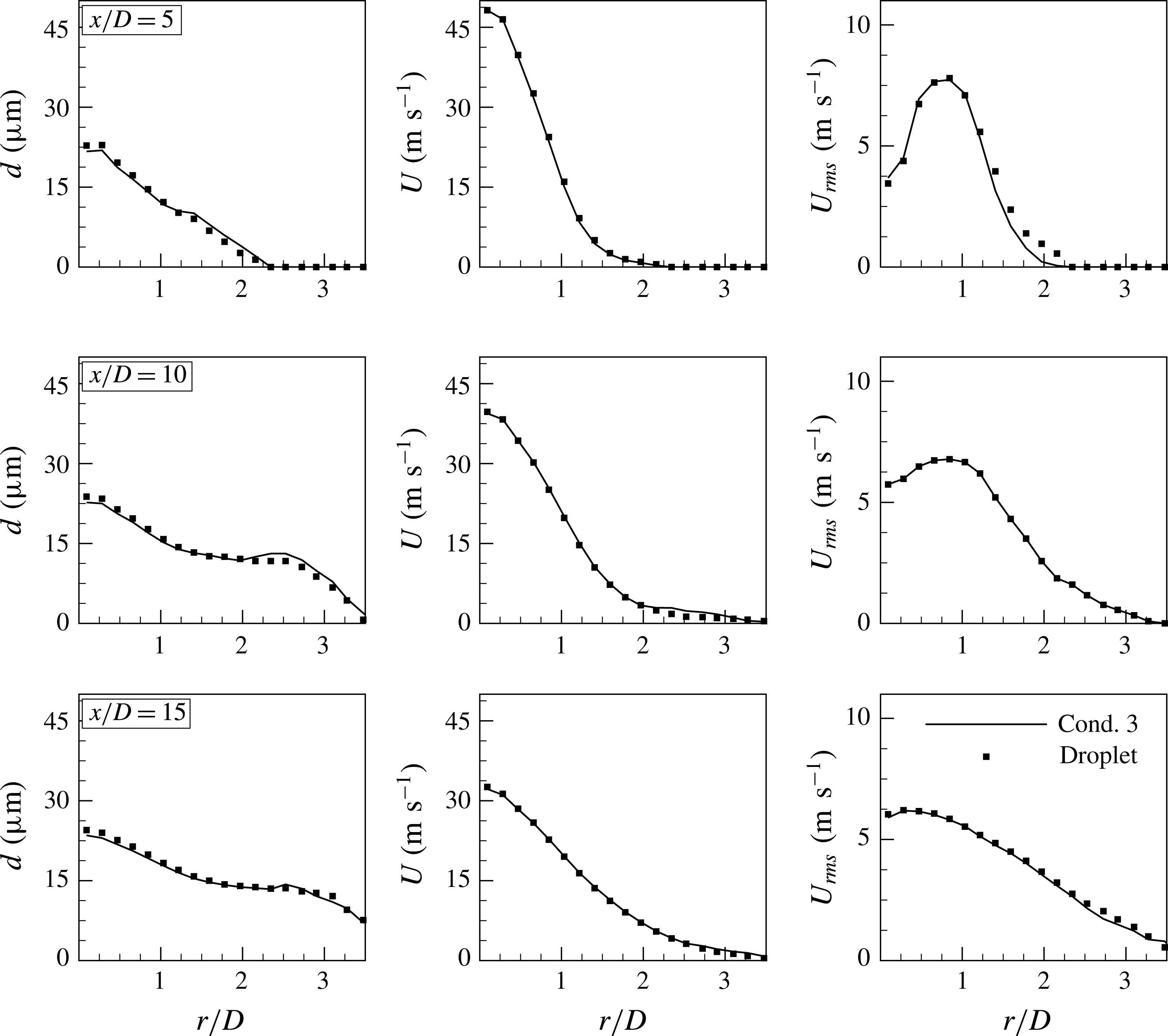
Figure 6 presents radial profiles of the mean diameter, the mean axial velocity and the velocity r.m.s. at three axial locations of $x/D=5$ , 10 and 15 for the coflow configuration in jet set I. The mean velocity and the its r.m.s. fluctuations are obtained by time averaging the droplet velocity for all sizes and shapes. It can be seen that the Cond. 3 notional particle solution is in excellent agreement with the baseline droplet simulation at all axial locations. As expected, the Cond. 7 solution fails to predict the correct dispersion, demonstrating the inability of using a single PDF-PBE class (i.e. a single Stokes bin) to represent the turbulent distribution over the full range of droplet sizes that are present.

Figure 7.

Radial profiles of the mean diameter, the mean velocity and the velocity r.m.s. in the coflow injector configuration with polydispersed oblate spheroidal droplets – the turbulent jet set I.

5.2.2 Non-spherical droplets

The PDF-PBE model is also applied to the dispersion of oblate spheroidal droplets with an aspect ratio of 0.5 in the coflow configuration injection in the turbulent jet set I. The initial droplet size distribution and the mass loading remain unchanged from the spherical-droplet-laden flows discussed in § 5.2.1. For simplicity, we neglect changes of the droplet orientation relative to the carrier flow and the drag coefficient is obtained using equations (2.7) and (2.8). This is considered adequate for the objectives of the current paper but with the proviso that, in practical applications, the orientation of droplets should be considered as it affects the drag coefficient and consequently the acceleration of the droplets (Loth Reference Loth2008). Figure 7 presents the PDF-PBE results in comparison with the baseline droplet simulation. Results are shown only for Cond. 3 in table 2. As expected, peak values of the mean diameter, the mean velocity and $U_{rms}$ change only marginally compared to the results for spherically shaped droplets. This is due to the fact that the same initial droplet size distribution was used in both sets of simulations. However, the level of radial dispersion increases for the oblate spheroids since the drag coefficient is higher compared with that for the spherical droplets. For instance, at $x/D=15$ and $r/D=3.5$ , the mean diameter obtained for the oblate spheroidal droplets is three times larger than for the spherical droplets. It can be seen that in comparison to the baseline droplet simulations the PDF-PBE predicts the radial profiles at all axial locations very well, confirming the PDF-PBE model with eight Stokes bins criterion works well for both spherical and non-spherical droplets.

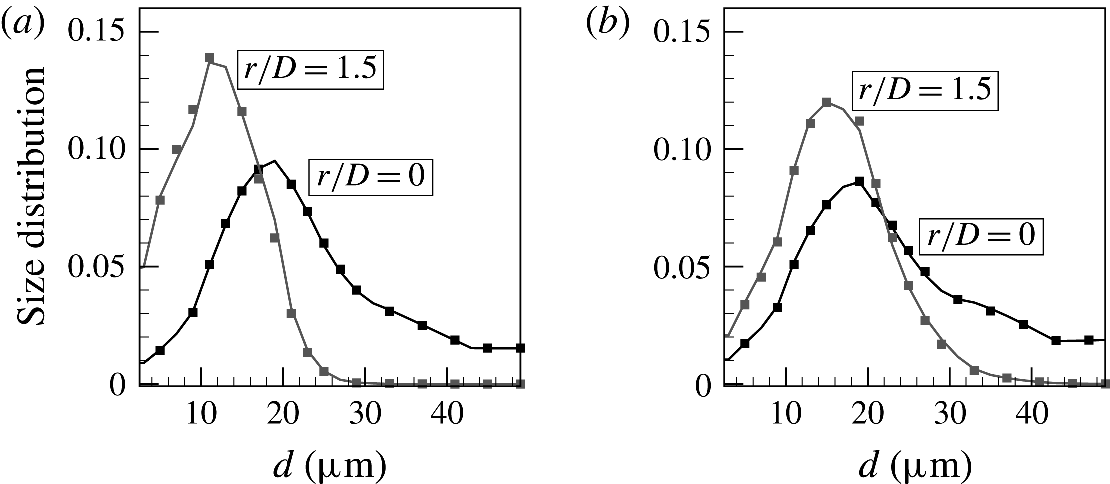
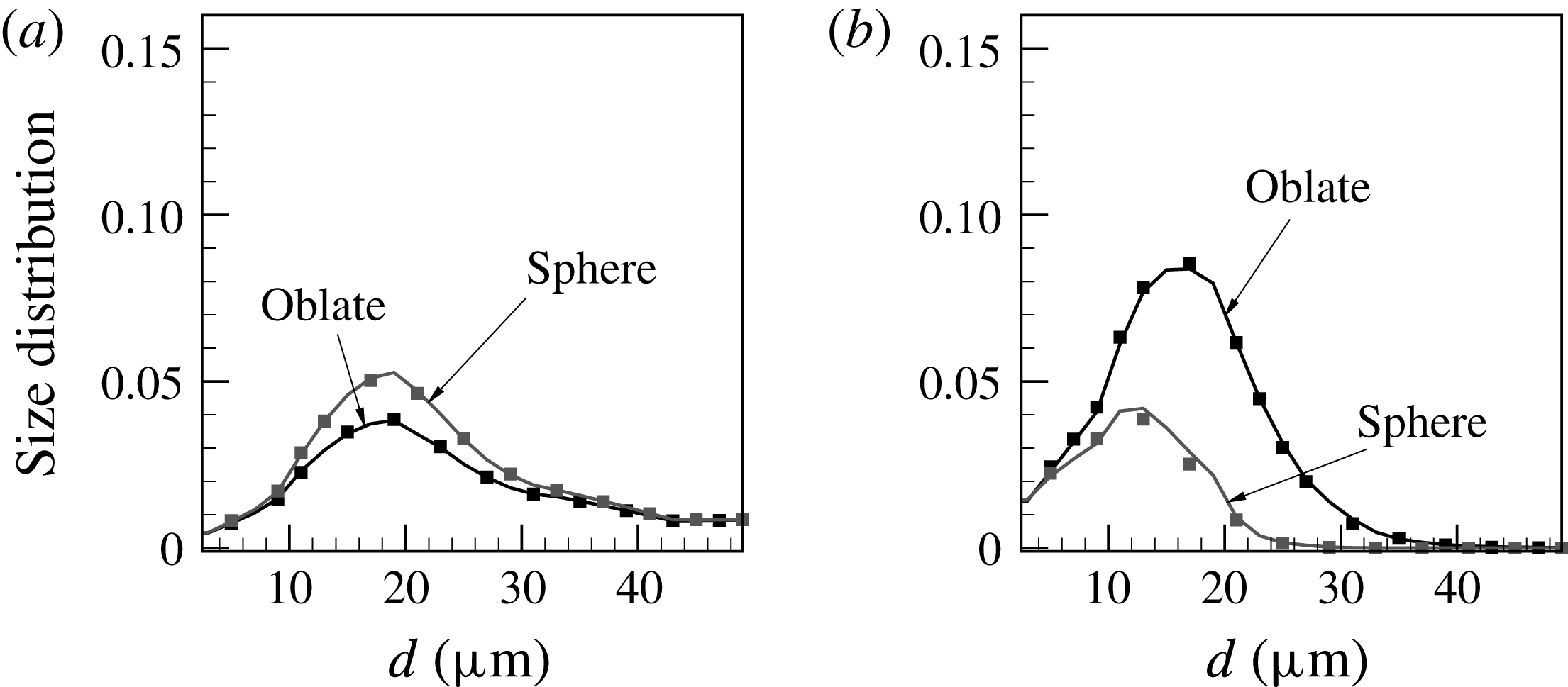
To shed more light on the difference between spherical and oblate spheroidal droplets, the mean droplet size distribution versus effective diameter is presented in figures 8(a) and 8(b). The results are for the coflow injector configuration. The droplet size distribution is computed at the two small regions marked by boxes shown on figure 2(a). Both regions are at the axial location of $x/D=15$ but two different radial locations of $r/D=0$ and 1.5, respectively. Several observations can be made.

Figure 8.

Mean droplet size distribution at $x/D=15$ and $r/D=0$ and 1.5 for (a) spherical and (b) oblate spheroidal droplets in the coflow injector configuration – the turbulent jet set I; solid line, Cond. 3 notional particle solution; symbol, baseline droplet solution.

1. (i) For both shapes, droplet size ranges from $1~\unicode[STIX]{x03BC}\text{m}$ to $50~\unicode[STIX]{x03BC}\text{m}$ near the centreline, whereas close to the shear layer ( $r/D=1.5$ ) the droplet size range is limited to maximum values of approximately $26~\unicode[STIX]{x03BC}\text{m}$ and $32~\unicode[STIX]{x03BC}\text{m}$ for spherical and oblate spheroidal droplets, respectively. This confirms that heavy droplets are simply convected downstream with only a slight radial dispersion detectable in their paths. This also demonstrates that oblate droplets with the same size as spherical droplets have shorter response times and hence a higher level of radial dispersion.

2. (ii) For both shapes, the location of the droplet size distribution peak shifts to the smaller size and, at the same time, the peak value also increases as the probe location moves from $r/D=0$ to 1.5. This indicates that light droplets follow the spreading of the carrier fluid trajectories and concentrate preferentially near the shear layer.

3. (iii) The spherical droplets reveal a more noticeable difference in the value and the location of the distribution peak between the two radial locations.

4. (iv) At both radial locations, PDF-PBE results for both shapes show excellent agreement with the baseline droplet simulations.

5.2.3 Spherical droplets — validation against the experimental data

The PDF-PBE model is now validated against the experiment to test its ability to predict dispersion of spherical droplets in a turbulent round jet (Kennedy & Moody Reference Kennedy and Moody1998) as described in § 4.2. The experiment was conducted for two droplet diameters of 60 and $90~\unicode[STIX]{x03BC}\text{m}$ . However, in the PDF-PBE simulation, we assume that an injected notional particle initially represents a range of droplet size from 10 to $90~\unicode[STIX]{x03BC}\text{m}$ with a constant interval of $10~\unicode[STIX]{x03BC}\text{m}$ . As explained above, a notional particle immediately splits into as many as required corresponding to the Stokes bin criterion. Since droplets do not alter the carrier-phase velocities and there is no interaction between droplets, the considered condition does not affect the dispersion of the 60 and $90~\unicode[STIX]{x03BC}\text{m}$ droplets but it allows us to test the Stokes binning method. Similarly, eight Stokes bins with $\unicode[STIX]{x0394}St=0.38$ are employed here while the lower and upper Stokes cutoff are updated to 0.5 and 120, respectively, in correspondence of the reported inlet Stokes range in the test case set II.

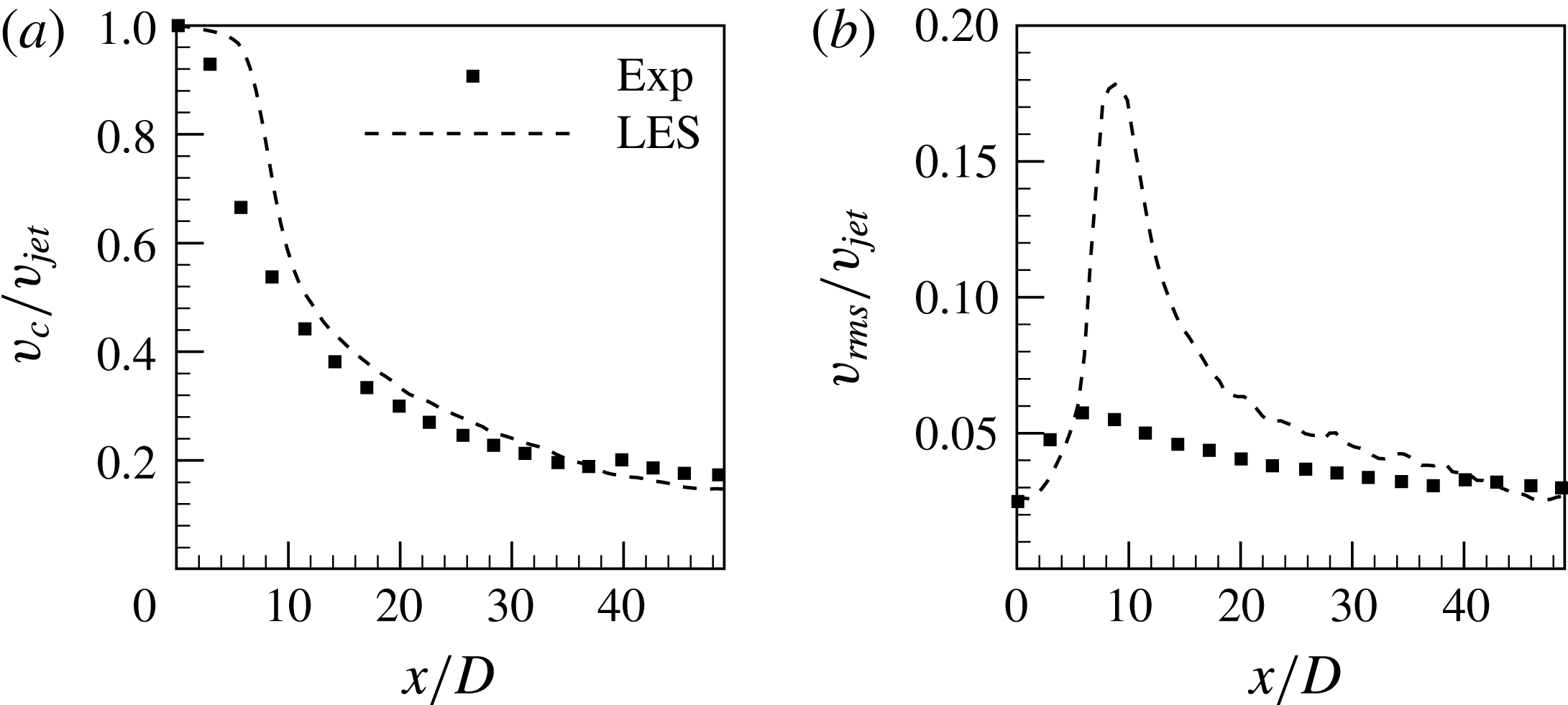
Figure 9 presents the centreline profiles of axial mean carrier-phase velocity, $v_{c}$ , and its r.m.s., $v_{rms}$ normalised by $v_{jet}$ . Overall, the agreement between the LES and the experiment is satisfactory. It can be seen that the LES mean velocity is slightly higher than the experiment at early stages while it agrees very well further downstream. This is consistent with the observation in figure 9(b) where the peak value of $v_{rms}$ is overpredicted. One possible reason may be due to the assumption of a uniform turbulent intensity across the inlet jet but that aspect cannot be further investigated since the experimental radial velocity r.m.s. profiles are not available. The turbulence model also plays a significant role in predicting the jet breakup point and hence more advanced turbulence models may improve results. However, it is worth noting a similar level of agreement was reported by Sun, Hewson & Lignell (Reference Sun, Hewson and Lignell2017) who employed a different turbulence model for simulation of the same jet. Although the accuracy of the predicted carrier phase has a significant impact on particle dispersion, we believe the LES accuracy is sufficient here since the disagreement in the carrier velocity r.m.s. is only observed at upstream locations of $x/D<20$ where the particle dispersion is small. It can be seen that the LES prediction is satisfactory further downstream where most of the particle dispersion occurs.

Figure 9.

(a) Normalised mean carrier flow velocity and (b) turbulence intensity along the centreline – the turbulent jet set II.

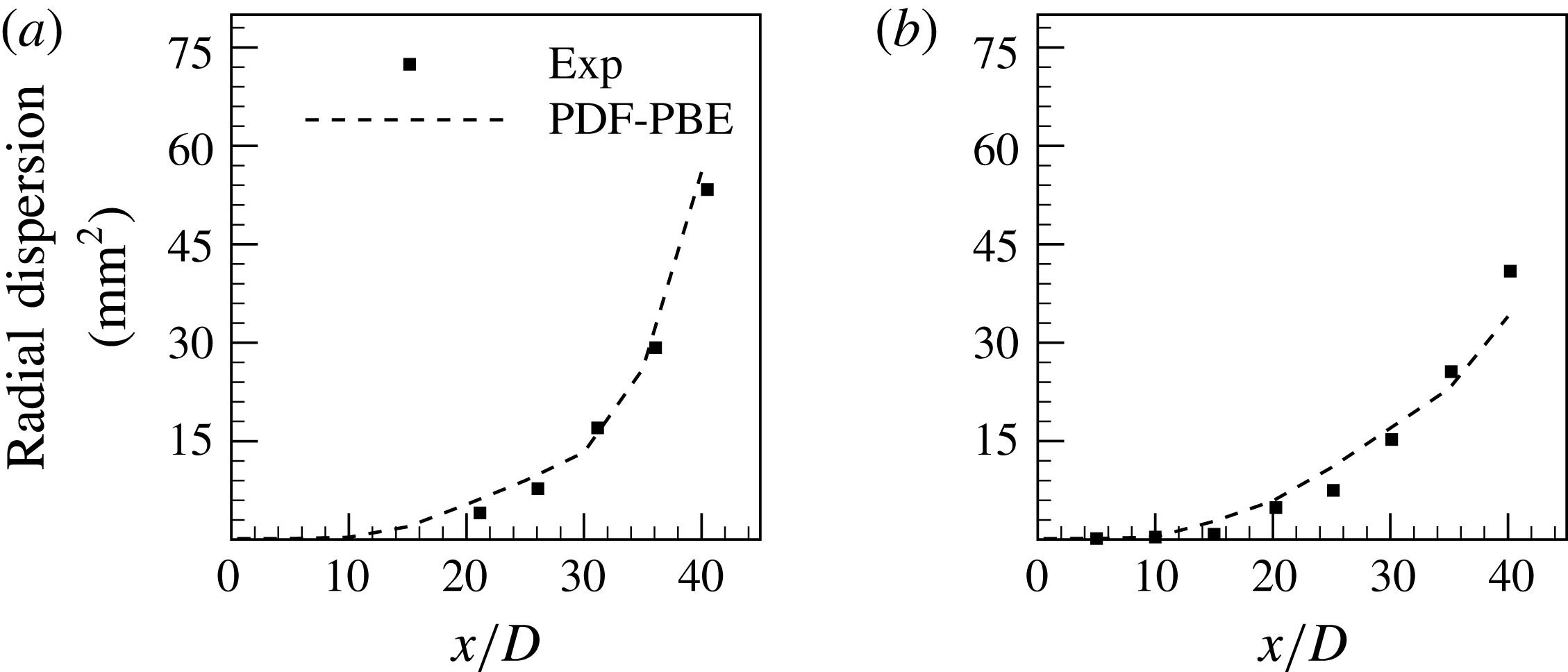
Figure 10 shows the dispersion of both 60 and 90  $\unicode[STIX]{x03BC}\text{m}$ droplets as a function of axial location normalised by the jet nozzle diameter. The dispersion is defined as the mean square displacement of the droplets from the jet centreline at a given axial location. As expected, the droplet dispersion increases with the jet evolution and its rate is steeper for smaller droplets. 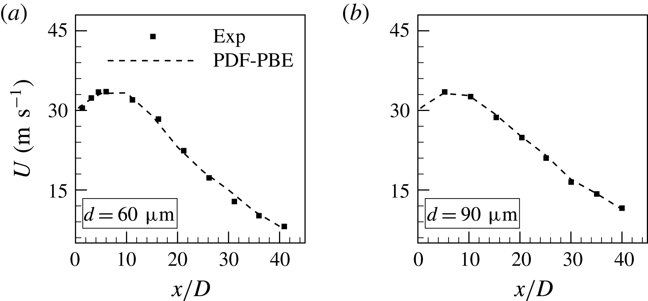The PDF-PBE reproduces the droplet dispersion very well although there is a slight overprediction at early stages for both 60 and $90~\unicode[STIX]{x03BC}\text{m}$ droplets. This can be due to the discrepancy observed in the predicted carrier flow velocities. Figure 11 presents the mean axial droplet velocities along the centreline. The agreement between the PDF-PBE and the experiment is excellent for both droplet sizes. Similar to the experiment, the droplet velocities initially increase, since they are injected at a lower velocity than the fluid, but later decrease as the droplets relax to the decaying carrier velocity. It is expected that the overpredicted carrier flow velocity r.m.s. leading to a discrepancy in the droplet velocity r.m.s. at early stages in the jet but unfortunately this cannot be further investigated here since the experimental data are limited to the mean values.

Figure 10.

Radial dispersion of (a) $60~\unicode[STIX]{x03BC}\text{m}$ and (b) 90  $\unicode[STIX]{x03BC}\text{m}$ droplets – the turbulent jet set II.

Figure 11.

Mean droplet velocities of (a) $60~\unicode[STIX]{x03BC}\text{m}$ and (b)  $90~\unicode[STIX]{x03BC}\text{m}$ droplets – the turbulent jet set II.

5.3 The PDF-PBE of polysized and polyshaped droplets

We now explore the PDF-PBE model for the combined dispersion of both polysized and polyshaped droplets. For this purpose, a combination of spherical and oblate spheroidal droplets are injected into the coflow injector configuration with the mean jet carrier velocity as described in § 4.1. The initial droplet size distribution is the same for both shapes and the total mass loading is $0.2~\text{g}~\text{s}^{-1}$ . In the PDF-PBE simulations, individual notional particles simultaneously carry both droplet size and shape information. Initially, a notional particle represents the entire range of droplet sizes and both shapes, however, it immediately splits into as many as eight bins to satisfy the Stokes binning criterion.

Figure 12.

Radial profiles of the mean diameter, the mean velocity and the velocity r.m.s. for polysized and polyshaped droplets in the coflow injector configuration – the turbulent jet set I.

Figure 12 presents the radial profiles of the mean diameter, the mean velocity and $U_{rms}$ at three axial locations; $x/D=5$ , 10 and 15. As expected due to the larger drag coefficient of the oblate spheroids than for the spheres, the mean level of radial dispersion in the present combined case is greater than for the case with spherical droplets only and less than the case with oblate spheroidal droplets only. As an example, at $x/D=15$ and $r/D=3.5$ , the mean diameter of polyshaped droplets is two times larger than it was in the case with just spherical droplets while its is approximately 60 % of the value obtained in the case with only spheroids. Excellent agreement can be observed between the PDF-PBE results and the baseline droplet simulation, confirming the PDF-PBE model based on the Stokes binning criterion successfully predicts the dispersion of a combined flow with polyshaped and polysized droplets.

The droplet size distribution conditioned on the shape at the axial location of $x/D=15$ and the radial locations of $r/D=0$ and 1.5 is illustrated in figure 13. The effects of droplet shape are clearly evident in this figure. Near the centreline and for both shapes, the droplet size range is from 1 to $50~\unicode[STIX]{x03BC}\text{m}$ whereas it decreases to less than $40~\unicode[STIX]{x03BC}\text{m}$ at $r/D=1.5$ . A narrower distribution span is evident for spherical droplets, which is consistent with monoshaped droplet simulations presented in figure 8. It is interesting that the distribution peak at $r/D=1.5$ is even lower than the peak near the centreline. However, the opposite is true for oblate spheroidal droplets. It can be seen that at $r/D=1.5$ the concentration of light oblate spheroidal droplets is significantly higher than it is for light spherical droplets. The opposite trend is observed near the centreline. This confirms that droplets with the same sizes but different shapes can show a noticeably different response to the carrier flow. A slight discrepancy between the Cond. 3 solution and the baseline droplet solution is observed at $r/D=1.5$ , however, the overall agreement is very good.

Figure 13.

Conditional mean droplets size distribution at the axial location of $x/D=15$ and the radial locations of (a) $r/D=0$ and (b) $r/D=1.5$ ; solid line, Cond. 3 notional particle solution; symbol, baseline droplet solution. Results are for the coflow injector configuration in the turbulent jet set I.

5.4 The PDF-PBE for breakage of polysized droplets

In this section, we investigate the PDF-PBE model for a case with a simple droplet breakage, as a pretext to future application of the PDF-PBE method to spray atomisation. For this purpose, a model for the source term, $w$ in equation (2.1) is required. It is important at this point to draw the distinction between droplet breakage, which is a physical process, and notional particle splitting into Stokes bins, which is a modelling tool. In the PDF-PBE approach proposed here, the modelling of droplet breakage does not necessitate the splitting the notional particles unless that droplet breakage has led to a violation of the criterion that $\text{d}St<\unicode[STIX]{x0394}St$ . As splitting of notional particles adds to the computational cost then avoiding it, where possible, is a significant computational efficiency measure.

In the context of PBE, Lasheras et al. (Reference Lasheras, Eastwood, Martınez-Bazán and Montanes2002) reviewed various stochastic breakage models which are dynamically related to the flow field through the breakage frequency, $f$ , and the local Weber number, $We=\unicode[STIX]{x1D70C}d_{p}|\boldsymbol{v}-\boldsymbol{U}|^{2}/\unicode[STIX]{x1D70E}$ , where $\unicode[STIX]{x1D70E}$ is the surface tension of the dispersed phase. For the purposes of this demonstration, a simplistic breakage model is used. We use $f=1/\unicode[STIX]{x1D70F}_{b}$ , where $\unicode[STIX]{x1D70F}_{b}$ is a characteristic breakage time scale which is assumed to be constant here. A droplet breaks into two identical daughter droplets if its Weber number is larger than a critical threshold, $We_{c}$ . In the droplet simulations with breakage, the mass is naturally conserved through the breakage since there is no restriction on the new droplet sizes. In the notional particle simulations with breakage, there are two approaches to ensure mass conservation determined by whether the droplet sizes are represented by either static or dynamics sections. In the first approach, the range of droplet sizes (on each notional particle) is discretised into sections which are static. If a larger sized droplet breaks into a smaller one whose size is in between two static sections then the newly formed droplet must be divided between the two sections with weightings selected under the constraint of mass conservation (Prakash, Bapat & Zachariah Reference Prakash, Bapat and Zachariah2003). In the second approach, the number of sections discretising the droplet size range is dynamic and new sections are added as needed. The static method leads to an artificial broadening of the predicted droplet size distribution but it is numerically efficient. The dynamic method does not produce artificial broadening but it has the potential to be computationally expensive, especially if used to model continuous size and shape changes, for example due to evaporation. Here the dynamic approach is adopted for its simplicity, but we do not discount the possibility that the static approach could be more practical approach in general. Here we conveniently adopt a threshold of $We_{c}=0.5$ as the breakage criterion for the coflow case with monoshaped and polysized droplets injected into the turbulent jet set I. This value, which is considerably smaller than that used elsewhere (Jones & Lettieri Reference Jones and Lettieri2010), was selected simply to produce a moderate level of breakage in the demonstration flow case considered here. The same value of $We_{c}$ is used in both the baseline droplet simulations and the notional particle simulations. The surface tension and the breakage time scale are $25.2~\text{mN}~\text{m}^{-1}$ and $10~\unicode[STIX]{x03BC}\text{s}$ , respectively.

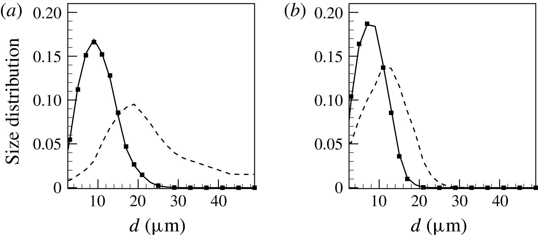
Figure 14 shows the droplet size distribution at the axial location of $x/D=15$ and the radial locations of $r/D=0$ and 1.5. Compared to the no-breakage condition (also shown and taken from figure 8 a), the droplet size range is notably narrower at both radial locations, particularly near the centreline where the maximum effective droplet diameter decreases to $25~\unicode[STIX]{x03BC}\text{m}$ from $50~\unicode[STIX]{x03BC}\text{m}$ . It can be seen that the location of the droplet size distribution peak shifts to the smaller size and, at the same time, the peak value significantly increases at both radial locations. PDF-PBE results show excellent agreement with the baseline droplet simulations when the droplet breakage is considered. This accuracy also comes at an affordable and controlled computational cost. Any increases in the number of notional particles in the PDF-PBE simulation is determined by the Stokes binning criterion and droplet breakage does not automatically lead to the need for additional notional particles. In the present set of simulations, the PDF-PBE modelling of droplet breakage is slightly less than 30 % of the cost of the droplet simulations.

Figure 14.

Mean droplets size distribution at the axial location of $x/D=15$ and the radial locations of (a) $r/D=0$ and (b) $r/D=1.5$ ; solid line, PDF-PBE with breakage (Cond. 3 notional particle solution); dashed line, baseline droplet solution without breakage; symbol, baseline droplet solution with breakage. Results are for the coflow injector configuration in the turbulent jet set I.