Introduction
Antarctic sea ice is an important component of the Southern Hemisphere (SH) climate system, largely through its modulation of atmosphere-ocean heat fluxes (e.g. Simmonds Reference Simmonds1981, Simmonds & Wu Reference Simmonds and Wu1993). West Antarctic sea ice trends may have a role in explaining the strong recent warming of the Antarctic Peninsula (Lachlan-Cope Reference Lachlan-Cope2005), and Southern Ocean sea ice variability may have global significance through its influence on the ocean circulation. Upwelling in the Southern Ocean is an important component of the Atlantic thermohaline circulation, the major cross-equatorial ocean current (e.g. Mikolajewicz Reference Mikolajewicz1998, Stossel et al. Reference Stossel, Yang and Kim2002). The heat, salinity and momentum fluxes that drive this upwelling are modulated by sea ice variability (e.g. Ludicone et al. Reference Ludicone, Madec, Blanke and Speich2008).
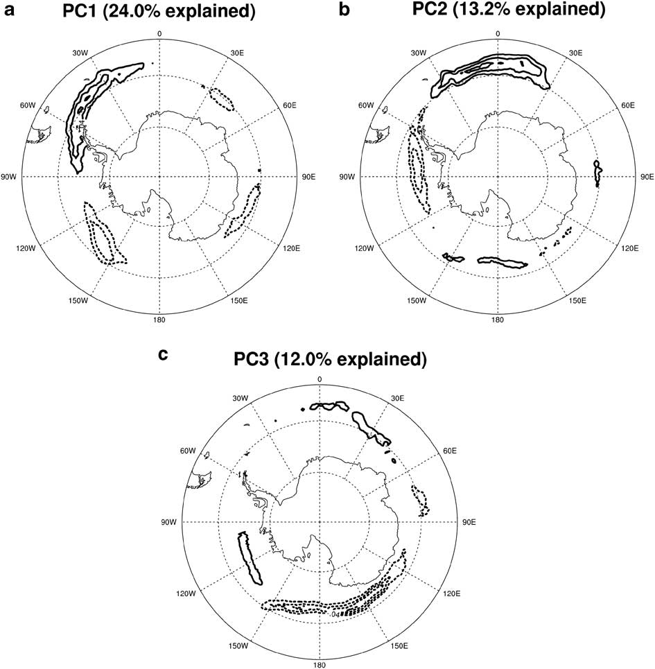
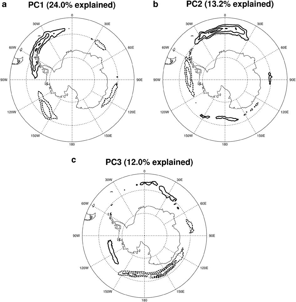
Patterns of sea ice variability are spatially heterogeneous in the SH, with maximum extents ranging from 55°S for the Ross and Weddell Sea sectors, to 65°S for the Amundsen and Bellingshausen Sea sectors. The greatest variance is also in the sectors of the Ross and Weddell seas. The three leading principal components (PCs) of sea ice concentration (SIC) explain approximately 24, 13 & 12% of total winter variability respectively, and are shown in Fig. 1. The opposing-phase relationship between sea ice in the Ross and Amundsen and Weddell/Bellingshausen seas shown in the first PC (Fig. 1a) is known as the Antarctic Dipole (Yuan & Martinson Reference Yuan and Martinson2000, Reference Yuan and Martinson2001). The Antarctic Dipole (ADP) also appears to represent the strongest mode of teleconnection with lower latitudes, and can be predicted by extreme anomalies of central tropical Pacific sea surface temperature (Yuan & Martinson Reference Yuan and Martinson2001). As well as dominating the interannual variability, the ADP is clear in long-term trends in SH sea ice. Since 1979, there has been a significant positive trend in Ross and Amundsen SIC and a negative trend in the Bellingshausen/Weddell, of approximately 4–10% per decade (Liu et al. Reference Liu, Curry and Martinson2004). Additionally, Stammerjohn et al. (Reference Stammerjohn, Martinson, Smith, Yuan and Rind2008) showed significant trends in the duration of sea ice cover. The greatest trends in annual ice duration are in the west Ross Sea (an increase of 1.8 months) and the southern Bellingshausen Sea (2.6 months shorter). The Bellingshausen Sea has also shown a reduction in extent of perennial sea ice over the same period (Stammerjohn et al. Reference Stammerjohn, Martinson, Smith, Yuan and Rind2008).
a. 1st, b. 2nd, and c. 3rd principal components of 1979–2006 July–September Southern Hemisphere SIC. Contour line spacing is 0.02 with no zero-line, negative contours are dashed.
Several studies have attempted to link sea ice variability to the major SH climate modes. Carleton (Reference Carleton1989) found that ice in the Ross and Weddell seas lagged tropical Pacific variability by several months, but results were inconclusive. Later work by Yuan & Martinson (Reference Yuan and Martinson2000) suggested that El Niño-Southern Oscillation (ENSO) accounted for 34% of variance in SH sea ice extent (SIE). The relationship with ENSO was concentrated in the Amundsen, Bellingshausen and Weddell Sea regions and projected onto the ADP pattern. Both Yuan & Martinson (Reference Yuan and Martinson2000) and Renwick (Reference Renwick2002) found that the greatest response was in the Amundsen Sea. Yuan & Martinson (Reference Yuan and Martinson2000) attributed this to the zonally asymmetric Hadley Cell response, which strengthens the Pacific Ferrell Cell, so that during El Niño events there is an anomalous northerly airflow suppressing ice extent in the Ross and Amundsen sectors. The inverse is true of the region close to the AP, resulting in increased extent in the Weddell/Bellingshausen sectors (Yuan Reference Yuan2004, Liu et al. Reference Liu, Curry and Martinson2004). The SH atmosphere also reacts to ENSO through the Pacific-South American mode (PSA, Renwick Reference Renwick2002, Yuan Reference Yuan2004). The PSA is a wave train forced by western tropical Pacific convection that propagates south-eastward, reaching its southernmost extent in a blocking high in the AP and Drake Passage region (Mo & Ghil Reference Mo and Ghil1987). During warm ENSO (i.e. El Niño) events, convection anomalies cause the PSA to shift in such a way that meridional air flow anomalies increase sea ice extent in the Weddell and Bellingshausen seas, and reduce sea ice extent in the Ross and Amundsen seas. Furthermore, Yuan & Martinson (Reference Yuan and Martinson2000) showed that correlations between surface air temperature (SAT) and SIE have distinct and different patterns: west Weddell SIE is correlated with an ENSO-like pattern of tropical Pacific SAT indicating a tropical Pacific teleconnection, whereas SIE in the Amundsen and Bellingshausen region are only correlated with local SAT. This result emphasizes the heterogeneity of sea ice variability, the importance of atmospheric temperature, and the teleconnection of Weddell Sea ice with the tropics.
The Southern Annular Mode (SAM) is the leading mode of atmospheric variability in the SH high and mid-latitudes. Several authors have suggested that it has an influence on SH sea ice variability (Hall & Visbeck Reference Hall and Visbeck2002, Liu et al. Reference Liu, Curry and Martinson2004). Model simulations suggest that when the SAM is in a strong positive phase and the circumpolar zonal winds are consequently increased, Ekman drift transports ice northward. This results in an increase in SIE, but a decrease in SIC close to the continent (Hall & Visbeck Reference Hall and Visbeck2002). However, observations indicate that the sea ice-response to SAM variability is more zonally heterogeneous. In the Ross and Amundsen sector, SIC away from the continent is increased during positive SAM phases due to Ekman transport, as predicted by the Hall & Visbeck (Reference Hall and Visbeck2002) model. In the Weddell and Bellingshausen sectors SIC cover is decreased by atmospheric warm advection, due to an anomalous cyclonic circulation west of the Drake Passage (Liu et al. Reference Liu, Curry and Martinson2004).
The sea ice response to La Niña events is the inverse of that for El Niño events, but tends to be stronger and more consistent over different events. Stammerjohn et al. (Reference Stammerjohn, Martinson, Smith, Yuan and Rind2008) suggested that this is due to the SAM modulation of high latitude ENSO-response, since a positive SAM phase causes the same ice anomalies as an El Niño event. Long term positive trends in both SAM and ENSO imply opposite effects on the observed ADP-pattern trends in sea ice. Liu et al. (Reference Liu, Curry and Martinson2004) used regression analysis to show that SAM-response is somewhat greater in magnitude than ENSO-response, and the observed ice trend is consistent with a positive SAM phase, which may be due to seasonal effects, ENSO is most active during November and December, when SH sea ice is retreating.
Recent work comparing the influence of the major climate modes on SH sea ice suggests that SIC variability is dominated by zonally asymmetric modes of variability, as opposed to the quasi-zonally symmetric SAM (Yuan & Li Reference Yuan and Li2008). The zonally asymmetric SH circulation is dominated by zonal waves one and three (ZW1 and ZW3), which combined explain almost all the mean spatial pattern of the SH troposphere (van Loon & Jenne Reference Van Loon and Jenne1972, Trenberth Reference Trenberth1980). Raphael (Reference Raphael2007) analysed autumn–winter sea ice variability with respect to ZW3, and found that when ZW3 was strong, southerly airflow was increased in the Weddell and Ross seas increasing SIC in those regions, and northerly airflow was increased in the Amundsen Sea with a resultant reduction in SIC. The pattern of variability closely resembled the third PC of winter sea ice variability (Fig. 1c), and was largely attributed to atmospheric thermal advection. ZW3 may also have an influence on regional sea ice dynamics. Massom et al. (Reference Massom, Stammerjohn, Lefebvre, Harangozo, Adams, Scambos, Pook and Fowler2008) showed that extreme ice compaction in the west AP during 2005 was due to a strong ZW3 pattern. The Raphael (Reference Raphael2007) study explicitly considered only the strength of the ZW3, and not the spatial variability. The research in this paper expands on that work by considering the spatial variability of the zonally asymmetric circulation. The influence of ZW1 on sea ice has not been analysed in detail, although a ZW1 signal on sea surface temperature has been shown for the west Antarctic region (Hobbs & Raphael Reference Hobbs and Raphael2007).
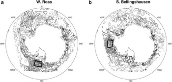
Liu et al. (Reference Liu, Curry and Martinson2004) showed that ENSO and SAM alone are insufficient to explain the observed ADP trend, while Lefebvre et al. (Reference Lefebvre, Goosse, Timmerman and Fichefet2004) showed that only for the Ross Sea were sea ice trends consistent with the long-term SAM trend. Lefebvre & Goosse (Reference Lefebvre and Goosse2008) used model and reanalysis data to confirm the importance of meridional airflow on sea ice variability, but they also showed that none of the recognized atmospheric modes were able to explain winter sea ice variability, averaged over the whole region. This result is not inconsistent with previous work, since as has been shown above the highly heterogeneous response to the major climate modes indicates that a single pattern that explains SIC variance throughout the Southern Ocean is probably not feasible. Figure 2 shows the winter SIC spatial autocorrelation between two regions showing strong recent trends: the west Ross and Bellingshausen seas. It is clear that despite their simultaneous trends and their mutual appearance in the 2nd PC of SIC, sea ice in the two regions is uncorrelated, a further indication that different processes drive their variability. This helps explain why previous studies have shown that large-scale circulation patterns fail to explain the observed trends in ice except at a regional level.
1979–2006 zero-lag correlation of local average SIC for a. west Ross Sea, and b. south Bellingshausen Sea, with July–September SIC throughout the Southern Ocean. Contour intervals are 0.1 and negative correlations are dashed. Statistically significant correlations are shaded.

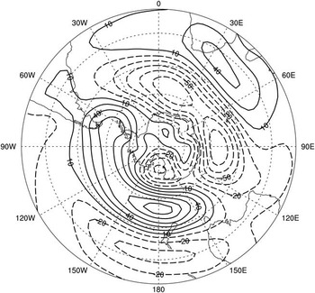
Hobbs & Raphael (Reference Hobbs and Raphael2009) showed that much of the high latitude tropospheric variability explained by ZW1 and ZW3 and by the PSA modes may be attributed to the variability of two persistent quasi-stationary anticyclones located in the Pacific and Drake Passage regions. They comprise an east anticyclone (at longitude 90°W) and a west anticyclone (at longitude 180°W), both have mean latitudes of 65°S (Fig. 3). This twin-anticyclone pattern is apparent in about 80% of monthly-mean fields examined. The variability of these anticyclones has been indirectly considered by previous researchers, through their representation in conventional decompositions, such as by principal component (e.g. SAM, PSA) or Fourier analysis (e.g. zonal waves). However, we propose that a clearer interpretation of the influence of zonally asymmetric dynamics is possible by considering the anticyclones separately, since firstly much of their variance is independent of each other, rather than as part of a single mode of climate variability as implied by PC or Fourier decomposition (Hobbs & Raphael Reference Hobbs and Raphael2009), and secondly local signals are not damped by far-field effects, as may be the case with large-scale decompositions. Additionally, the PC method returns temporal information for the relative strength of each individual component only, thus much information regarding spatial variability is lost.
1979–2007 mean zonal anomaly of NCEP/NCAR reanalysis 500 hPa geopotential height.

In this paper the variability of SH sea ice is analysed at seasonal and interannual time scales with respect to variability in the strength and location of the sub-polar anticyclones. It is shown that the east anticyclone has a significant influence on early winter SIC in a pattern that projects on the first PC of SH SIC, and the west anticyclone has an influence on late winter sea ice with a signal that resembles the second PC of SIC.
Method
Sea ice concentration data are available from January 1870, but data from the early part of this record are based on very sparse observations and are thus unreliable, hence the analysis here is restricted to the period from which satellite sea ice data from passive microwave retrievals were available. Sea ice concentration data are taken from the HadISST1 1979–2006 monthly mean sea ice concentration data (Rayner et al. Reference Rayner, Parker, Horton, Folland, Alexander, Rowell, Kent and Kaplan2003). Data are mapped onto a 1° x 1° latitude/longitude grid. Since the HadISST1 inception, the SIC data have been widely and successfully used for both observation-based research and model simulations. Monthly SIE data were derived from the HadISST1 SIC, by taking the lowest latitude at each longitude at which the SIC was ≥ 0.3. Where no sea ice is present at a certain longitude, the SIE was set to the latitude of the HadISST land mask (for the seasons of greatest interest in this study this is unlikely to be an issue).
Daily and monthly ice motion data are from the 1979–2006 Polar Pathfinder Daily 25 km EASE-Grid Sea Ice Motion Vectors, provided by the National Snow and Ice Data Centre Distributed Active Archive Centre (NSIDC DAAC). The daily motion data are derived from buoys and the AVHRR, SMMR and SSM/I space borne instruments. The retrieval algorithm is based on tracking the movement of identified ice features (e.g. an ice floe), and is considered reliable away from the ice edge, where a modelling of complex ice dynamics would be required (Fowler Reference Fowler2003). Information on data quality is provided in the case of monthly-mean fields as the number of daily observations used for that month’s mean, and in the case of daily fields as the square root error variance. The data are interpolated onto a 25 x 25 km2 equal area grid, and gridpoints more than 1250 km from the nearest observation are flagged.
The primary atmospheric data were from monthly-mean fields of the NCEP/NCAR 40-year reanalysis (NRA, Kalnay et al. Reference Kalnay, Kanamitsu, Kistler, Collins, Deaven, Gandin, Iredell, Saha, White, Woollen, Zhu, Leetmaa and Reynolds1996), provided by the NOAA/OAR/ESRL PSD, Boulder, Colorado, USA, from their web site at http://www.cdc.noaa.gov/ (accessed 10 March 2009). Wind and temperature data at the 925 hPa level were used as a proxy to calculate thermal advection at the surface. In any atmospheric reanalysis, surface fields may be influenced by surface-process model parameterizations, hence 925 hPa was chosen as the lowest atmospheric level that is relatively immune to model influences (Kalnay et al. Reference Kalnay, Kanamitsu, Kistler, Collins, Deaven, Gandin, Iredell, Saha, White, Woollen, Zhu, Leetmaa and Reynolds1996, Uppala et al. Reference Uppala, Kållberg, Simmons, Andrae, Da Costa-Bechtold, Fiorino, Gibson, Haseler, Hernandez, Kelly, Li, Onogi, Saarinen, Sokka, Allan, Andersson, Arpe, Balmaseda, Beljaars, van de Berg, Bidlot, Bormann, Caires, Chevallier, Dethof, Dragosavac, Fisher, Fuentes, Hagemann, Hólm, Hoskins, Isaksen, Janssen, Jenne, McNally, Mahfouf, Morcrette, Rayner, Saunders, Simon, Sterl, Trenberth, Untch, Vasiljevic, Viterbo and Woollen2005). The mid-troposphere circulation was represented by the 500 hPa geopotential height. Several studies have reported spurious trends in the NRA data for the high latitude SH, principally due to the introduction of satellite data for periods after the late 1970s (e.g. Marshall Reference Marshall2002, Reference Marshall2003). Since this analysis is restricted to the post-satellite era the data should be relatively free from this effect, nevertheless, linear trends were removed from all data (including atmospheric fields, climate indices and sea ice data) prior to correlation or composite analysis. Additionally, results were compared with equivalent estimates made using the 1980–2001 European Centre for Medium Range Weather Forecasting 40-year reanalysis (ERA-40) obtained from their web site at http://www.ecmwf.int/research/era/do/get/era-40 (accessed 4 April 2009, Uppala et al. Reference Uppala, Kållberg, Simmons, Andrae, Da Costa-Bechtold, Fiorino, Gibson, Haseler, Hernandez, Kelly, Li, Onogi, Saarinen, Sokka, Allan, Andersson, Arpe, Balmaseda, Beljaars, van de Berg, Bidlot, Bormann, Caires, Chevallier, Dethof, Dragosavac, Fisher, Fuentes, Hagemann, Hólm, Hoskins, Isaksen, Janssen, Jenne, McNally, Mahfouf, Morcrette, Rayner, Saunders, Simon, Sterl, Trenberth, Untch, Vasiljevic, Viterbo and Woollen2005). Several studies have compared SH fields from the NRA and ERA data, and although there are differences in the major fields especially over the polar regions, the datasets agree reasonably well in their representation of the SH atmosphere. It has been suggested that for SH high latitudes the more recent ERA-40 is an improved dataset (e.g. Marshall Reference Marshall2003, Bromwich et al. Reference Bromwich, Fogt, Hodges and Walsh2007), but at the time of writing data were only available up to August 2002 and did not provide as long a coverage period as the NRA data.
A set of time series describing the strength and location of the sub-polar anticyclones were described in Hobbs & Raphael (Reference Hobbs and Raphael2009). These time series are: the west anticyclone height anomaly (HGTW, measured in geopotential meters, gpm), the west anticyclone longitude (LONW, degrees east), and the east anticyclone height and longitude (HGTE and LONE). For approximately 10% of the months analysed the zonal anomaly field was identified as showing a single-anticyclone pattern, akin to the canonical ZW1 pattern. Further research is proposed to explore the physical interpretation of these single-anticyclone patterns, but since this investigation is focused on the signal due to the east and west anticyclones these anomalous months were removed from the data. Analysis of the time series revealed that the anticyclones’ strength and location were second-order stationary for the seasons February–April (FMA), May–July (MJJ), August–October (ASO) and November–January (NDJ, Hobbs & Raphael Reference Hobbs and Raphael2009), hence these seasons are primarily used in this investigation.
Cross-correlations were considered significant where the correlation coefficient was statistically different from zero at the 0.05 significance level. In some cases, after removal of ‘flagged’ months the number of independent observations was less than 20 and the use of a parametric test would be unreliable, so significant correlations were estimated using a resampling approach. First-order autoregressive (AR(1)) models were fit to the SIC data and anticyclone time series and 100 000 random time series were generated with the same sample size, SD and AR(1) parameters. The anticyclone-derived random series were correlated with each other, and then with the SIC-derived random series. For both cases the probability density functions (PDFs) of the cross-correlations were analysed. The PDFs were approximately Gaussian with a mean of zero, and from this correlations of 0.4 were found to have two-tailed statistical significance at the 0.05 level, whether for the anticyclone time series correlated with each other or with the SIC data. Where data have been composited by the anticyclone height time series, high composite months were those where the height was more than 0.5 SD greater than the mean, and low composite months were those where the height was more than 0.5 SD less than the mean. Where data have been composited by the anticyclone longitude time series, high composite months were those where the longitude was more than 0.5 SD east of the mean location, and low composite months were those where the longitude was more than 0.5 SD west of the mean.
Results
Correlations between sea ice concentrations and the anticyclones
Figure 4 shows the correlation coefficients between the anticyclone time series and SIC, for selected seasons. The strength of the west anticyclone (HGTW) is significantly correlated with sea ice for the late winter (ASO, Fig. 4a) and early summer (NDJ, not shown) seasons. The patterns are qualitatively similar for both seasons, but with a stronger and more widespread correlation for ASO. There are significant correlations for the anticyclone leading and lagging sea ice, but correlations are more persistent and stronger when sea ice lags the anticyclone, indicating an atmosphere-to-ocean relationship. The correlations are strongest at lag-0, the pattern shown in Fig. 4a. The pattern is characterized by negative correlations in the Ross Sea and East Antarctic, and positive correlations off the coast of Dronning Maud Land, east of the Weddell Sea (a region referred to in the remainder of this paper as DML). The correlation with the west anticyclone longitude (LONW) is also strongest for ASO (Fig. 4b). The relationship is stronger than for HGTW, with significant correlations in the Ross Sea region leading LONW by one month and persisting up to a lag of five months (i.e. subsequent JFM sea ice). Correlations are most widespread with OND SIC (Fig. 4b). The HGTW and LONW time series have a statistically significant positive cross-correlation during ASO (r = 0.33), and the similarity in their SIC correlation patterns could in part be an expression of that covariance. However, the maximum correlations are approximately similar for each time series (r = c. 0.6), showing that height/longitude covariance cannot entirely explain the indicated SIC-response to west anticyclone variability.
Correlation of late winter west anticyclone with HadISST SIC, for a. ASO HGTW with ASO SIC (lag 0), b. ASO LONW with OND SIC (i.e. lag 2), c. MJJ HGTE with MJJ SIC, and d. MJJ LONE with MJJ SIC. Contour intervals are 0.2 and negative contours are dashed. Regions where correlation is statistically significant at the 0.05 level are shaded.

As with the west anticyclone, the east anticyclone strength (HGTE) and longitude (LONE) are significantly correlated with the SIC. For both east anticyclone time series, the strongest correlation was for autumn–early winter (MJJ, Fig. 4c & d). MJJ is the season of greatest ice growth and conditions during this period have a significant impact on maximum SIE/SIC at the end of winter. The east anticyclone strength (Fig. 4c) and longitude (Fig. 4d) show similar but inverse patterns of correlation, the strongest signals being in the Weddell, Amundsen, Bellingshausen and DML sectors. The patterns are very similar to the 1st PC of SH SIC (Fig. 1a), with an increase in SIC in the Amundsen Sea and between 0 and 45°E, and a decrease in the Weddell Sea and west AP region when the east anticyclone is in a strong and eastern phase. This is also similar to the SIC response to ENSO-variability (e.g. Liu et al. Reference Liu, Curry and Martinson2004), which given the approximate location of the east anticyclone may indicate that it responds to tropical Pacific variability through the PSA. There are also significant correlations with SIC for ASO strength and NDJ longitude, with similar but weaker patterns to those shown in Fig. 4. The correlation with SIC is somewhat stronger for the longitude compared to strength, and the inverse patterns of correlation are consistent with the correlation between LONE and HGTE time series (r = -0.75 for MJJ). Both time series were correlated with a time series of Weddell Sea SIC defined as the monthly average SIC for the spatial domain 40–50°W, 65–70°S. The correlation for longitude was indeed higher than for the strength (r = -0.78 for LONE, compared to r = 0.59 for HGTE). After accounting for the HGTE-LONE covariance, the Weddell SIC-HGTE correlation becomes just 0.42 (correlations of 0.4 or higher are significant at the 0.05 level). It therefore seems that the apparent correlation between east anticyclone strength and sea ice is largely a function of the longitude signal. Thus, in the following discussion results for the HGTE, which are qualitatively the inverse of those for LONE, are not considered.
The sub-polar anticyclones exert most influence on sea ice during early winter (MJJ) and early spring (ASO), which are key seasons for the advance and retreat of seasonal sea ice. To explore a possible link with the seasonal evolution of sea ice, the MJJ east anticyclone time series were correlated with ice advance and duration data, and the ASO west anticyclone time series were correlated with ice retreat and duration data, kindly supplied by Sharon Stammerjohn. The duration data are derived from the 1979–2006 SSM/I and SSMR sea ice concentration data, where the day of advance for each pixel is defined as the first day of each year after 15 February when SIC rises above 15% for at least five consecutive days, and the retreat is the first day following advance that the SIC dips below 15% for at least five consecutive days (Stammerjohn et al. Reference Stammerjohn, Martinson, Smith, Yuan and Rind2008).
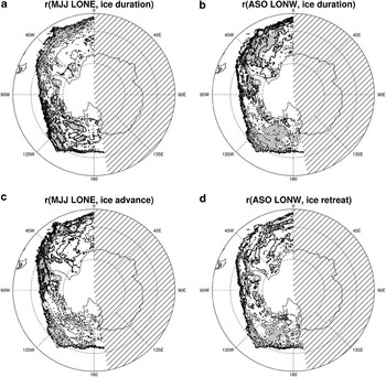
The anticyclone longitudes are both significantly correlated with ice duration (Fig. 5). Correlations with ice duration are spatially similar to the correlations with SIC shown in the figures. When the MJJ east anticyclone tends to an eastern phase (i.e. high LONE), ice advance is later in the Weddell and Bellingshausen seas, and is earlier in the Ross and Amundsen Sea sectors (Fig. 5c). The magnitude and pattern of LONE correlation with ice advance is closely matched in magnitude and distribution by the correlation with duration (Fig. 5a), such that later (earlier) advance results in a shorter (longer) period of ice cover. The ASO LONW correlations show a similar pattern, such that ice duration is increased (decreased) in regions showing a positive (negative) correlation with SIC (Fig. 5b & d). It is interesting to note that for the Weddell Sea, the LONW correlation with retreat is much weaker and less coherent than the correlation with duration, suggesting that since the link between ice duration and the west anticyclone cannot be solely explained by the timing of autumn ice advance, thus the anticyclone must also influence spring ice retreat.
1979–2006 correlations between SH ice duration date and the sub-polar anticyclones for a. MJJ LONE and ice duration, b. ASO LONW and ice duration, c. MJJ LONE and ice advance, and d. ASO LONW and ice retreat. Contour intervals are 0.2 and negative contours are dashed. Regions where correlation is statistically significant at the 0.05 level are shaded and hashed regions show areas where data were unavailable.

In summary, during late autumn–early winter (MJJ), the longitude of the east anticyclone is related to a pattern of SIC response that projects strongly onto the first PC of winter SIC, the Antarctic Dipole. During late winter–spring (ASO), variability in both the strength and longitude of the west anticyclone influence SIC in the Ross Sea. Correlations with SIE follow the same pattern (Hobbs & Raphael Reference Hobbs and Raphael2009), with decreased SIE in the Weddell Sea and Drake Passage region and increased SIE in the Amundsen Sea and east of the Weddell Sea when the east anticyclone is in a strong and eastern phase. The west anticyclone strength and longitude both show similar patterns that are consistent with the distribution of SIC concentrations, with positive correlations in the Amundsen Sea and DML sectors, and negative correlations in the Ross Sea.
One difficulty with using cross-correlation as an analysis tool is the contamination of lead-lag correlation signals by the serial autocorrelation of sea ice. Statistically significant correlations were found for sea ice both leading and lagging the sub-polar anticyclone time series. The relative strengths of the lead and lag correlations indicate that the anticyclones largely lead SIC, suggesting a possible atmosphere-to-ice forcing, rather than vice versa. To confirm the atmosphere-to-ice relationship indicated by the lead-lag signal, anticyclone time series were derived from two model simulations made using the NCAR CCSM3.0 coupled climate model (Collins et al. Reference Collins, Bitz, Blackmon, Bonan, Bretherton, Carton, Chang, Doney, Hack, Henderson, Kiehl, Large, McKenna, Santer and Smith2006). Realistic maximum and minimum sea ice climatologies were derived from 1978–2000 HadISST daily sea ice concentration data, where the maximum (minimum) climatology for each month was taken from years with the maximum (minimum) Antarctic sea ice cover for that month. The climatologies were then used in place of the model’s dynamic sea ice component, and the simulation was run for 150 years. Anticyclone time series were calculated for each model run as described in the previous section for the seasons of interest (i.e. MJJ and ASO), and the time series for the two forcing scenarios were compared using Student’s t- and F-tests respectively. There were no significant differences in the means or variances for either the MJJ east or the ASO west anticyclones showing that the anticyclones are insensitive to sea ice variability, which is further evidence of an atmosphere-to-ocean forcing.
Mechanisms of anticyclone forcing of sea ice
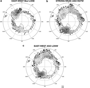
As discussed in the introduction, atmospheric circulation can influence sea ice distribution either thermodynamically through atmospheric thermal advection, or dynamically by wind-driven ice drift. Considering first the importance of dynamic forcing, difference maps of sea ice motion composited by LONE, HGTW and LONW are shown in Fig. 6. Compared to a western phase, when the east anticyclone is in an eastern phase (Fig. 6a), the climatological south-westerly ice flow from the Weddell Sea is increased, but south-westerly ice motion is decreased in the Bellingshausen Sea, despite the fact that both regions show the same SIC-response to LONE (Fig. 4d). The HGTW and LONW sea ice motion composites (Fig. 6b & c) both show increases in the climatological Ross Sea outflow and north-eastward flow near 0°E when the anticyclone is relatively strong and/or eastward. The mean longitude of the west anticyclone is approximately 180°W, so that the northward anticyclone airflow occurs over the Ross Sea (Hobbs & Raphael Reference Hobbs and Raphael2009). When the west anticyclone is relatively strong, northerly airflow over the Ross Sea is thus increased. When the anticyclone shifts east, the maximum pressure gradient of the anticyclone moves closer to the Ross Sea, and again northward airflow is increased there.
East–west composite difference in sea ice motion (m s-1), composited by a. MJJ LONE time series, b. ASO HGTW time series, and c. ASO LONW time series.

Establishing a link between sea ice motion and SIC is difficult to quantify, since areas of ice convergence/divergence may not necessarily cause a change in the sea ice concentration. Where ice motion causes convergence of ice mass into a region, rafting of the ice may mean that there is little effect on the areal concentration of ice. This could only be confirmed by including ice thickness data. Where ice motion causes divergence of ice from a region, the result may be to maintain a region of open water, or polynya. Latent-heat polynyas are important regions of sea ice production, since ocean-atmosphere heat flux is high compared to the surrounding ice-covered ocean. The consequent ocean cooling causes production of ice, which in the case of persistent polynyas is transported away by ice drift, and there is no influence on the SIC (e.g. Wu et al. Reference Wu, Budd and Allison2003). Thus, the response of SIC to both convergence and divergence is difficult to interpret, without a thorough treatment of heat flux and ice thickness data beyond the scope of this study. Instead, a statistical treatment of the role of ice motion on SIC variability is used here.
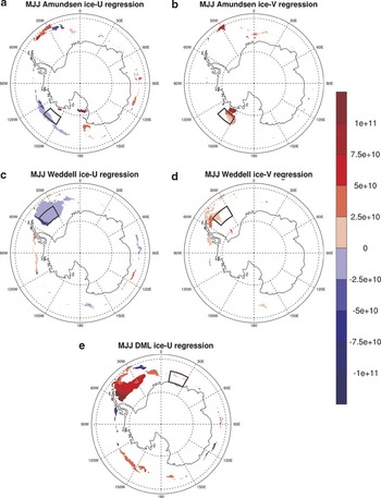
Time series were generated of total sea ice cover for regions showing a significant correlation with LONE, and were then regressed against ice motion for the MJJ season. The regions were the Amundsen Sea (68–72°S, 130–150°W), the Weddell Sea (65–70°S, 30–50°W), and the DML sector (67–70°S, 20–30°E). There is a positive relationship between Amundsen Sea ice and meridional ice motion, indicating northward transport of ice into the sector by the meridional Ross Sea outflow (Fig. 7a). Conversely, there is also a negative relationship with zonal flow, such that ice is transported out of the sector by eastward ice motion (Fig. 7b). Figure 6a shows that an eastward shift in the east anticyclone corresponds to a simultaneous decrease in both meridional ice flow into, and zonal flow out of that region. The Amundsen regression coefficients in Fig. 7a & b for zonal and meridional flow are similar in magnitude, as are the zonal and meridional ice motion responses to east anticyclone variability. Hence the opposing zonal and meridional effects of ice motion response to the east anticyclone must largely cancel each other out, resulting in little net signal in ice cover. A similar situation occurs in the Weddell sector (Fig. 7c & d), where the increased Weddell outflow caused by an eastward shift in the anticyclone (Fig. 6a) causes a zonal flow decrease and a meridional flow increase in ice cover. However, in the Weddell Sea the zonal flow seems to have a slightly greater influence on ice cover than the meridional flow, so ice motion may explain some of the negative anticyclone-sea ice correlation in Fig. 4d. Ice cover in the DML sector is positively correlated with zonal drift in the Weddell Sea, suggesting a significant transport of Weddell ice to the sector (Fig. 7e), but there is no significant relationship with meridional flow (not shown). Hence, increased Weddell outflow seems to transport ice eastwards from the Weddell Sea to the DML sector, possibly explaining the positive correlation with DML ice and east anticyclone longitude (Fig. 4d).
MJJ regression coefficient (m2 ms-1) between ice motion and sea ice cover for a. Amundsen Sea (zonal flow), b. Amundsen Sea (meridional flow), c. Weddell Sea (zonal flow), d. Weddell Sea (meridional flow), and e. DML (zonal flow). The spatial domain of the sector is indicated by a black polygon, and only areas with a statistically significant correlation between ice cover and motion are shaded.

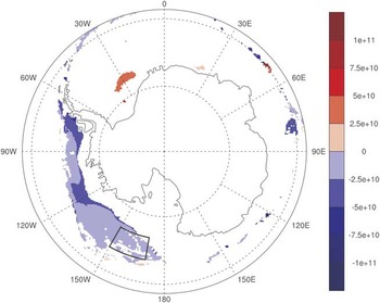
Time series were also generated of total areal ice cover for the regions of west anticyclone-SIC correlation: the Ross Sea (65–70°S, 150–170°W), the Amundsen Sea (68–72°S, 95–115°W), and the Bellingshausen Sea (67–71°S, 75–95°W), which were then regressed against the ice motion data for the ASO season (note that to capture the region of greatest sea ice correlation, the spatial domains were not exactly the same as those used in the MJJ analysis above). Figure 8 shows the sea ice-response to zonal ice motion for the Ross Sea sector, where ice is negatively correlated with HGTW and LONW (Fig. 4a & b). Although there is no significant link between sea ice and the meridional component (not shown), ice cover is reduced by increased zonal flow, which transports ice eastward away from the Ross Sea sector. Figure 6b & c shows that zonal ice flow is increased when the east anticyclone is relatively strong and/or east, the relationship between ice cover and ice motion is consistent with the negative correlation between the anticyclone and SIC. Neither the Amundsen nor the Bellingshausen Sea sectors (not shown) have significant correlations with ice motion, hence a physical mechanism other than wind-driven ice motion must be responsible for the correlations between SIC and the west anticyclone.
As for Fig. 7, but showing ASO regression coefficient between zonal ice motion and sea ice cover for the Ross Sea sector.

Overall, the anticyclones seem to modulate ice outflow in the Ross, Amundsen and Weddell seas. However, only the MJJ ice in the DML sector and ASO ice in the Ross Sea show sea ice motion responses that are consistent with the SIC correlations with the anticyclones. For the other regions, either this ice motion seems to have little influence on observed SIC, or the zonal and meridional responses to the anticyclones oppose each other. Hence, while some of the correlations between the anticyclones and SIC may be explained by wind-driven ice motion, it is unlikely to be the primary mechanism.
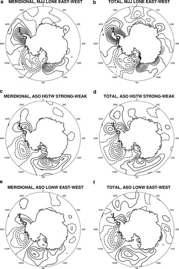
Estimates of 925 hPa atmospheric thermal advection (ATA) were composited by the LONE, HGTW and LONW time series (Fig. 9). For all the time series, the patterns of warm/cold advection over the Ross and Amundsen seas are consistent with their respective correlations with SIC (Fig. 4), and are consistent with geostrophic circulation around an anticyclone. The ATA pattern composited by MJJ east-anticyclone longitude shows that when the anticyclone is in a western phase, northerly airflow in the AP region is reduced and hence so is warm advection to the Bellingshausen and Weddell seas (Fig. 9a). Over the Amundsen Sea where SIC is positively correlated with LONE, a western phase (i.e. low LONE) results in an increase in warm advection and a concomitant decrease in SIC. Comparison of the east, west and neutral composites of ATA (not shown) indicates that the ATA signal is strongest when the east anticyclone is west of its mean location (i.e. low LONE), compared to the response when it is further east. When the west anticyclone is strong, there is increased poleward (i.e. warm) flow west and equatorward (i.e. cold) flow east of the anticyclone’s mean location (Fig. 9c), explaining the HGTW signal. As the anticyclone moves east to west these meridional currents also shift, hence when LONW is high (i.e. the anticyclone is east of its mean location) warm advection is increased further east and cold advection is decreased further west (Fig. 9e). Figure 9b, d & e show that the total thermal advection-responses (i.e. both the zonal and meridional components), are mostly attributable to meridional advection.
925 hPa atmospheric thermal advection composite differences integrated over the 3-month season (K), for a. MJJ meridional ATA composited by LONE, b. MJJ total ATA composited by LONE, c. ASO meridional ATA composited by HGTW, d. ASO total ATA composited by HGTW, e. ASO meridional ATA composited by LONW, and f. ASO total ATA composited by LONW. Contour intervals are 50 K, dashed contours indicate cold advection and solid contours indicate warm advection.

The analysis was repeated using the 1979–2001 ERA-40 925 hPa temperature and wind data (not shown), and the results were found to compare well for the Ross and Amundsen seas with the NRA results. However, there is poor agreement between the two datasets for the region running from the Antarctic Peninsula to about 60°E.
Relationships between the stationary anticyclones and sea ice trends
Late 20th century sea ice trends have been observed largely in the western hemisphere, the region of sub-polar-anticyclone sea ice signal (Liu et al. Reference Liu, Curry and Martinson2004). Due to the serial autocorrelation of winter sea ice, both the east anticyclone (with greatest SIC in autumn–early winter) and the west anticyclone (with greatest SIC-response in late winter) could have an influence on the observed sea ice trends. For the 1980–2001 period, the only robust trend in the anticyclones was a westward shift of 1° yr-1 for the ASO west anticyclone (Hobbs & Raphael Reference Hobbs and Raphael2009). This is consistent with the observed trends in late winter SIC, since west Ross Sea region (here defined as 150–180°W, 60–65°S) shows both a significant negative correlation with LONW, and a significant trend of 7.2% per decade for ASO. Simple regression was used to estimate the ASO SIC response to LONW as -0.8% per °E, hence it seems that most of the estimated SIC trend in that region (6.4% per decade) may be attributable to the western shift of warm, northerly airflow related to the west anticyclone. This result has potentially important implications for explaining the local increased sea ice cover in the Ross Sea which is at odds with an increase in surface temperature, and which cannot be explained by trends in the SAM (Liu et al. Reference Liu, Curry and Martinson2004).
There were no robust trends in the east anticyclone, despite strong observed trends in SIC in the region of east anticyclone influence. Meridional thermal advection is the primary mechanism by which the anticyclones influence sea ice, hence although the lack of east anticyclone trends suggests there has been no change in the meridional airflow associated with it, a change in the meridional temperature gradient would imply a change in strength of meridional thermal advection between the mid and high latitudes. Thus, we suggest the hypothesis that the east anticyclone could have a role in transporting mid-latitude warm anomalies to the west Antarctic region. Steig et al. (Reference Steig, Schneider, Rutherford, Mann, Comesino and Shindell2009) presented results that show a significant late 20th century warming in west Antarctica, outside the Antarctic Peninsula region which is influenced by SAM variability. This warm region corresponds to the approximate longitudes of poleward airflow due to the east anticyclone.
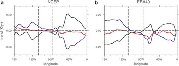
The western hemisphere linear trends in MJJ surface air temperature at mid- and high-latitudes (50 & 65°S respectively) are shown in Fig. 10, where the region of poleward advection due to the east anticyclone is denoted by vertical dashed lines. The two datasets show a similar general pattern, with high latitude warming in the west Pacific region and cooling in the Atlantic sector (blue lines), and generally weak trends at mid latitudes (red lines). However, the magnitude of trends do not agree well and there are several local features in the trends that are not common to both datasets, e.g. a mid latitude cooling in the ERA-40 data at 75°W that is not matched by the NCEP data. A common feature of both datasets is the relatively small difference between high and low latitude trends in the region of east anticyclone-induced poleward airflow, compared to the rest of the western hemisphere (black lines). This result is consistent with significant local meridional mass exchange due to the east anticyclone, since mixing would reduce meridional temperature differences. However, given the poor agreement between the datasets this result is not robust, and unfortunately the region of interest shown by the vertical dashed lines has no station data for validation.
1979–2001 MJJ linear trend by longitude in near-surface air temperature (K yr-1) for a. NCEP, and b. ERA-40 reanalysis datasets. Red line indicates trend at 50°S, blue 65°S, and black line indicates 50–60°S difference. Vertical dashed lines denote the mean region of poleward airflow due to the east anticyclone.

Discussion and conclusions
The Pacific sub-polar anticyclones’ strength and location both act to modulate sea ice distribution in a pattern that corresponds to the leading principal components of SH sea ice. During late autumn–early winter (MJJ), the longitude of the east anticyclone is related to a pattern of SIC response that resembles the first PC of winter SIC, the Antarctic Dipole. During late winter–spring (ASO), variability in both the strength and longitude of the west anticyclone work together to cause a SIC response concentrated in the Ross Sea. The response appears to be largely due to the anticyclones’ influence on meridional airflow, so modulating the distribution and strength of atmospheric thermal advection to the Ross, Amundsen, Bellingshausen and Weddell seas. Circulation anomalies related to the anticyclones’ variability also have an influence on ice motion, which may explain the correlation with SIC in the Dronning Maud Land sector, and may also partially explain the Ross Sea correlations. However, elsewhere the patterns of anticyclone correlation with SIC are not well explained by ice motion, leading to the conclusion that, within the limits of the analysis, thermal advection is the dominant mechanism by which the anticyclones influence ice cover.
A caveat of these results is the relatively simplistic treatment of sea ice advection, which in the absence of long-term ice thickness data relies on statistical inferences.
The first PC of sea ice shown in Fig. 1 closely resembles the estimate of sea ice response to ENSO (Liu et al. Reference Liu, Curry and Martinson2004). Since the east anticyclone variability is also linked to SIC PC1, and is also related to the PSA1 mode (Hobbs & Raphael Reference Hobbs and Raphael2009), it is reasonable to suggest that the east anticyclone has a role in explaining the teleconnection of tropical Pacific variability to the SH high latitudes. However, it should be noted that the season when the east anticyclone has the strongest influence on ice is MJJ, whereas SH ENSO-teleconnections tend to be most important later in the winter. Future work will explore the dynamics of the anticyclones, including their relationship with the tropical Pacific. It is hoped that the potential role of the anticyclones in transferring ENSO-variability to the high latitude SH will be clearer.
Regression analysis suggests that most of the positive trend in Ross Sea late winter sea ice cover may be attributed to a western shift in the west anticyclone. Further work is required to confirm this mechanism, but this initial result may shed important light on one part of the spatially heterogeneous pattern of recent Antarctic sea ice trends. The east anticyclone does not have a robust trend, but a hypothesis is proposed here that poleward transport of lower latitude warming due to the east anticyclone could lead to local West Antarctic warming. Trend patterns in both reanalysis datasets are consistent with this, but in the absence of reliable SAT observations for the Southern Ocean this hypothesis is difficult to test.
Acknowledgements
This work was funded jointly between the National Science Foundation’s grant ATM-0327268 and the UCLA Chancellor’s Dissertation Year Fellowship. NCEP/NCAR reanalysis data were provided by the NOAA PSD (http://www.cdc.noaa.gov), ERA-40 reanalysis data were provided by the ECMWF (http://www.ecmwf.int), and Pathfinder sea ice motion data was provided by NSIDC (http://nsidc.org/data/pathfinders/index.html). The authors give special thanks to Sharon Stammerjohn for provision of her sea ice duration data, and for several helpful discussions. The authors also thank the reviewers for their comments which have improved this manuscript.