1 Introduction
Dusty plasmas are ionized gases containing small (nanometre to
 $\unicode[STIX]{x03BC}$
m sized), solid particulates, or dust grains. In low temperature laboratory dusty plasma experiments, the grains are generally charged negatively by plasma collection because the electrons are more mobile than the ions. The dust acoustic, or dust density, wave is a low frequency collective mode associated with the dynamics of the dust grains (Rao, Shukla & Yu Reference Rao, Shukla and Yu1990). These waves have been observed in dusty plasma experiments both in the terrestrial laboratory and under microgravity conditions (Merlino Reference Merlino2014). The dust acoustic wave generally has a frequency
 ${\lesssim}$
the dust plasma frequency
 $\unicode[STIX]{x1D714}_{\text{pd}}$
and phase speed much smaller than the ion thermal speed (Shukla & Mamun Reference Shukla and Mamun2002). In typical dusty plasma experiments, these waves can have frequencies in the range of 10 Hz, wavelengths in the range of millimetres and phase speeds
 $c_{d}$
in the range of cm
 $\text{s}^{-1}$
.
It is thought that dust density waves can be excited by an ion flow relative to the dust (e.g. Rosenberg Reference Rosenberg1996; Joyce, Lampe & Ganguli Reference Joyce, Lampe and Ganguli2002). In laboratory dusty plasma experiments, there can be an ion flow due to a balance between acceleration by an electric field that confines the dust grains, and deceleration by collisions with neutrals. Kinetic theories of the linear ion–dust streaming instability have often invoked shifted Maxwellians to describe the ion velocity distribution (e.g. Rosenberg Reference Rosenberg1996; Molotkov et al.
Reference Molotkov, Nefedov, Torchinskii, Fortov and Khrapak1999; Fortov et al.
Reference Fortov, Khrapak, Khrapak, Molotkov, Nefedov, Petrov and Torchinsky2000; Piel et al.
Reference Piel, Klindworth, Arp, Melzer and Wolter2006). Recently, Kählert (Reference Kählert2015) considered the linear theory of this instability using a non-Maxwellian ion velocity distribution. This type of distribution can arise when ions are accelerated by a uniform electric field and decelerated by drag due to charge-exchange collisions (Lampe et al.
Reference Lampe, Rocker, Joyce, Zhdanov, Ivlev and Morfill2012). Charge-exchange collisions can be a dominant ion collision process in laboratory dusty plasmas with e.g. noble gases (see Semenov, Khrapak & Thomas Reference Semenov, Khrapak and Thomas2017). The form of the ion distribution function was determined by Lampe et al. (Reference Lampe, Rocker, Joyce, Zhdanov, Ivlev and Morfill2012) using Monte Carlo (MC) simulations and analysis, based either on a constant collision frequency or constant cross-section model. It was shown that, for a constant collision frequency model, the equilibrium ion distribution can be expressed as an analytic function of the ion thermal Mach number
 $M_{\text{th}}=U_{i}/v_{n}$
, where
 $U_{i}$
is the mean ion drift speed and
 $v_{n}$
is the thermal speed of the neutrals. The distribution of ion velocities in the streaming direction (i.e. the direction of the electric field) has a non-Maxwellian form which deviates substantially from a shifted Maxwellian for larger
 $M_{\text{th}}$
: the distribution has a slower exponential decay and is broader, with its width (i.e. ‘temperature’) increasing with
 $M_{\text{th}}$
(Lampe et al.
Reference Lampe, Rocker, Joyce, Zhdanov, Ivlev and Morfill2012).
A linear kinetic theory analysis of the ion–dust streaming instability was given in Kählert (Reference Kählert2015), using an ion susceptibility based on this non-Maxwellian ion distribution. It was found in Kählert (Reference Kählert2015) that the maximum growth rate of the instability tends to decrease compared to theories using a shifted-Maxwellian ion distribution. This decrease is more pronounced for lower ion collision rates and higher Mach numbers; in addition, there can be a shift in the wavelength of the most unstable mode. The decrease of the growth rate and shift in wavelength was attributed to the higher weighting of kinetic effects due to a broadened ion distribution in the non-Maxwellian case. In the limit of large ion collision rates, both models appear to yield similar results.
In this paper, we investigate the effect of a non-Maxwellian ion velocity distribution on the development of the ion–dust streaming instability, using one-dimensional (1-D) particle-in-cell (PIC) simulations. The results are compared with those for a shifted-Maxwellian ion distribution. In both cases, the ions are subject to a uniform background electric field and undergo collisions with neutrals. In the non-Maxwellian case the collisions are charge-exchange collisions modelled with a constant collision frequency (e.g. Lampe et al.
Reference Lampe, Rocker, Joyce, Zhdanov, Ivlev and Morfill2012). In the shifted-Maxwellian case the collisions are modelled by a Langevin operator which tends to thermalize the ion distribution (e.g. Quest et al.
Reference Quest, Rosenberg, Kercher and Dutreix2016). Because the linear growth rate of ion-dust streaming instability depends on quantities such as the ion drift speed and collision rate, we consider several values of the ion thermal Mach number
 $M_{\text{th}}$
and both a lower and higher ion collision rate. Section 2 discusses the model plasma and the simulation approach. Section 3 presents the results of the simulations, and § 4 gives a brief summary.
2 Model and simulation approach
2.1 Model
The model system is a weakly ionized plasma composed of electrons, singly charged ions, negatively charged dust grains of uniform radius
 $R$
(and thus uniform charge) and neutral atoms. The condition of overall charge neutrality is
 $$\begin{eqnarray}\displaystyle n_{e}+Z_{d}n_{d}=n_{i}. & & \displaystyle\end{eqnarray}$$
Here the subscripts
 $e,i,d$
refer to electrons, ions and dust, respectively, and
 $Z_{d}$
is the charge state of the dust, which is assumed constant. The background neutral gas has density
 $n_{n}\gg n_{i}$
, and we assume that the temperature of the gas
 $T_{n}$
is room temperature. The ordering of the particle species temperatures is
 $T_{e}\gg T_{n}$
, as is typical in low temperature dusty plasma experiments where the electron temperature can be a few eV. Typically, the ion temperature is near the gas temperature. (Note however, that the non-Maxwellian ion distributions that we will consider have high energy tails that essentially lead to higher effective ion temperatures compared to shifted-Maxwellian distributions, but which are still smaller than
 $T_{e}$
.)
There is a uniform background electric field
 $E_{0\,\boldsymbol{x}}$
which generates drifts in the charged particle species, with the drift velocity approximately given by
 $\boldsymbol{U}_{j}=q_{j}\boldsymbol{E}_{0}/m_{j}\unicode[STIX]{x1D708}_{j}$
, where
 $q_{j}$
and
 $m_{j}$
are the charge and mass of each charged particle species, and
 $\unicode[STIX]{x1D708}_{j}$
is the collision frequency of each charged species with the background neutrals. The system is one-dimensional, with the wavevector
 $\boldsymbol{k}$
in the direction of the ion drift which is in the
 $x$
-direction. We consider the frame where initially there is no dust drift, and we neglect collisions of the dust with neutrals. While realistically the dust particles would also collide with neutrals, which would tend to cool and thermalize the dust distribution, this assumption allows us to isolate the effects of non-Maxwellian ions.
Typical dusty plasmas under laboratory conditions (e.g. Merlino Reference Merlino2014) or microgravity conditions (e.g. Fortov et al.
Reference Fortov, Morfill, Petrov and Thoma2005; Khrapak et al.
Reference Khrapak, Ratynskaia, Zobnin and Usachev2005) generally involve
 $\unicode[STIX]{x03BC}$
m size grains, which have a negative charge state
 $Z_{d}$
of the order of a thousand, and a mass
 $m_{d}$
of the order of
 $10^{12}$
proton masses. Because of the very small dust charge-to-mass ratio, and correspondingly small ratio of the dust plasma frequency,
 $\unicode[STIX]{x1D714}_{\text{pd}}$
, to the ion plasma frequency,
 $\unicode[STIX]{x1D714}_{\text{pi}}$
, it is very time consuming to run a numerical simulation of the development of the ion–dust streaming instability for realistic dusty plasma parameters. However, the essential physics can reasonably be captured by using a set of reduced parameters which reflect the requisite ordering of physical quantities. This includes having (i) a dust charge-to-mass ratio much smaller than that of the ions, (ii) a dust acoustic speed
 $c_{d}$
much smaller than the ion thermal speed and (iii) a wave frequency
 $\unicode[STIX]{x1D714}$
(which is typically
 ${\lesssim}\unicode[STIX]{x1D714}_{\text{pd}}$
) much smaller than the ion collision frequency
 $\unicode[STIX]{x1D708}_{i}$
. Thus we require (i)
 $Z_{d}m_{i}/m_{d}\ll 1$
, (ii)
 $c_{d}\ll v_{i}$
and (iii)
 $\unicode[STIX]{x1D714}_{\text{pd}}\ll \unicode[STIX]{x1D708}_{i}$
. We will also require
 $\unicode[STIX]{x1D714}_{\text{pd}}/\unicode[STIX]{x1D714}_{\text{pi}}\ll 1$
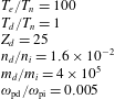
. A set of reduced parameters that satisfy these conditions are given in table 1 along with the additional assumption that the ion–neutral collision frequency is
 ${\gtrsim}0.1\unicode[STIX]{x1D714}_{\text{pi}}$
which is typical for low temperature dusty plasmas (see, e.g. Winske Reference Winske2004).
Reduced parameters.

2.2 Simulation approach
The simulations were performed with a 1-D electrostatic PIC code with periodic boundary conditions. The plasma species in the PIC simulation consists of singly charged ions that stream in the
 $x$
-direction relative to multiply charged, heavy dust grains that are stationary in the simulation reference frame. Because
 $T_{e}\gg T_{n}$
and
 $n_{i}>n_{e}$
, we assume the electrons are Boltzmann distributed and just provide charge neutrality.
The ions and dust are treated as particles, but only the ions collide with the background neutrals, with a collision frequency
 $\unicode[STIX]{x1D708}_{i}$
. The magnitude of the background electric field
 $\boldsymbol{E}_{0}=E_{0}\boldsymbol{x}$
is set such that the corresponding electric force on the ions balances the ion–neutral collisional force to yield a particular ion mean drift velocity
 $\boldsymbol{U}_{i}=U_{i}\boldsymbol{x}$
at the beginning of the simulation. Thus, for the background electric field we use the approximate expression
 $E_{0}=m_{i}\unicode[STIX]{x1D708}_{i}U_{i}/e$
.
We will consider two different forms of the initial ion velocity distribution. One form is a non-Maxwellian with a mean drift speed
 $U_{i}$
, which arises from ion acceleration in the uniform electric field and deceleration by ion charge-exchange collisions. Imposing the thermal Mach number
 $M_{\text{th}}=U_{i}/v_{n}$
, where
 $v_{n}=(T_{n}/m_{i})^{1/2}$
, is sufficient to set the shape of the distribution as well as the velocity moments (Lampe et al.
Reference Lampe, Rocker, Joyce, Zhdanov, Ivlev and Morfill2012). In the simulation code, the initial ion distribution is established by setting the collision frequency and driver electric field (which determines
 $M_{\text{th}}$
), then time advancing the ions with fixed electric field for several collision times. Once the ions have reached the desired equilibrium state, the self-consistent fields as well as dust dynamics are initiated. The charge-exchange collisions are implemented using a well established Monte Carlo process (e.g. Birdsall Reference Birdsall1991; Lampe et al.
Reference Lampe, Rocker, Joyce, Zhdanov, Ivlev and Morfill2012). The fixed collision frequency yields a probability that a specific macro-particle is scattered during any given time step. If it is scattered, the particle is randomly assigned a new velocity based on the normal distribution of the neutral population.
For comparison, the other form of the initial ion distribution is a shifted Maxwellian with drift speed
 $U_{i}$
. This form has been used in several numerical simulation studies of ion–dust streaming instabilities, generally with lower drift speeds (see e.g. Winske Reference Winske2004; Fu & Scales Reference Fu and Scales2012). A Langevin scattering operator, with a constant ion collision frequency, is used to model collisional effects (Gillespie Reference Gillespie1993); the collisions tend to thermalize and cool the ions to the temperature of the neutrals. The numerical implementation of the scattering operator is well established and is described in Lemons et al. (Reference Lemons, Lackman, Jones and Winske1995) and Winske & Rosenberg (Reference Winske and Rosenberg1998).
A nonlinear Poisson equation is used to obtain the self-consistent wave potential
 $\unicode[STIX]{x1D719}$
. Consistent with the Boltzmann approximation, the electron number density
 $n_{e}$
assumes the form
 $n_{e}=n_{e0}\text{e}^{e\unicode[STIX]{x1D719}/T_{e}}$
. Together with the ion and dust charge densities, the Poisson equation can then be solved by standard iterative means (Hockney & Eastwood Reference Hockney and Eastwood1981).
Quantities in the simulation are normalized to ion quantities at the beginning of the simulation, but with the temperature given by the neutral particle temperature which is assumed constant. Thus, temperatures and drift speeds are normalized to
 $T_{n}$
and the associated neutral thermal speed
 $v_{n}=(T_{n}/m_{i})^{1/2}$
. Length scales are normalized to the ion Debye length
 $\unicode[STIX]{x1D706}_{\text{in}}$
evaluated at
 $T_{n}$
and the initial ion density
 $n_{i0}$
, while time scales are normalized to the ion plasma frequency
 $\unicode[STIX]{x1D714}_{\text{pi}}$
evaluated with
 $n_{i0}$
. The wave electrostatic potential energy
 $e\unicode[STIX]{x1D719}$
is normalized to
 $T_{n}$
(in energy units), and the wave electric field
 $\tilde{E}$
is normalized to
 $E_{r}=T_{n}/e\unicode[STIX]{x1D706}_{\text{in}}$
. It follows that the electric field energy density in simulation units is
 $\tilde{E}^{2}/2E_{r}^{2}=E^{2}/(8\unicode[STIX]{x03C0}n_{i0}T_{n})$
. In this 1-D simulation, the system length is
 $128\unicode[STIX]{x1D706}_{\text{in}}$
and is divided into 256 computational cells for the
 $M_{\text{th}}=1$
case and into 128 cells for the higher Mach numbers. To reduce the numerical noise, the ions and dust are modelled assuming approximately 4 million macro-particles for each species for
 $M_{\text{th}}=1$
, and 2 million particles for higher Mach numbers. For all runs the time step
 $\unicode[STIX]{x0394}t$
and the ion collision frequency
 $\unicode[STIX]{x1D708}_{i}$
obey
 $\unicode[STIX]{x0394}t\unicode[STIX]{x1D708}_{i}=0.01$
.
For the simulations discussed in the following, we use the reduced set of dimensionless parameters given in table 1. For the case of a shifted-Maxwellian ion velocity distribution, we assume that the initial ion temperature
 $T_{i}=T_{n}$
. For the non-Maxwellian ion distribution, it can be shown that the effective ion temperature varies as
 $(1+M_{\text{th}}^{2})$
and that the heat flux is
 $2M_{\text{th}}^{3}m_{i}v_{n}^{3}$
, consistent with the asymmetric high-energy tail. The initial dust velocity distribution is taken as a Maxwellian with zero drift.
3 Simulation results
Because the linear growth rate of the ion–dust streaming instability depends on quantities such as the ion drift speed and the ratio
 $\unicode[STIX]{x1D708}_{i}/\unicode[STIX]{x1D714}_{\text{pi}}$
(which can be
 ${\gtrsim}0.1$
in laboratory experiments), we will consider several values of these quantities. We will consider the following three cases of ion thermal Mach speed
 $M_{\text{th}}=U_{i}/v_{n}$
at the beginning of the simulation:
 $M_{\text{th}}=1$
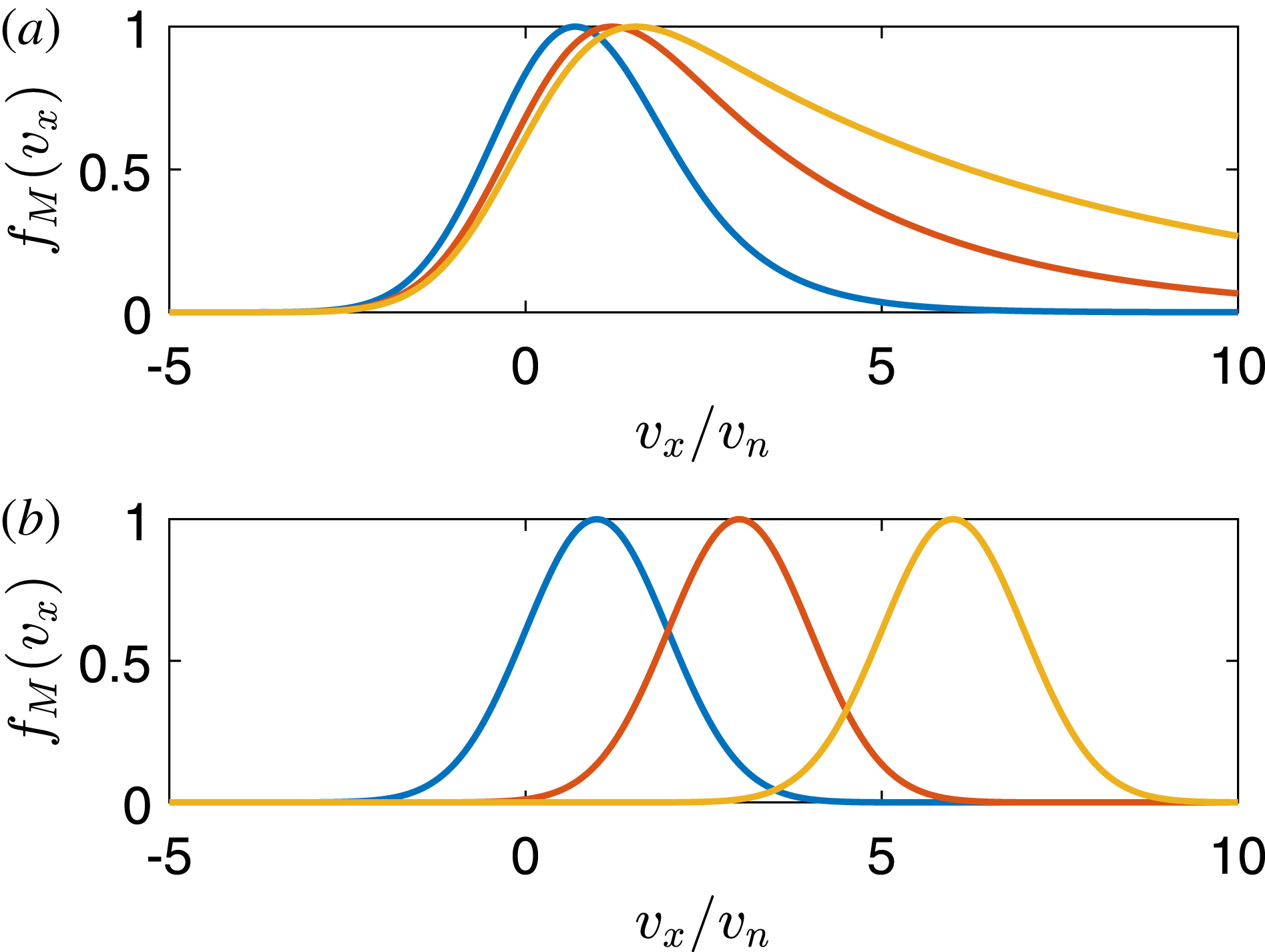
, 3 and 6 (to be referred to as Cases I, II and III, respectively). Figure 1 shows initial ion distribution functions for these values of
 $M_{\text{th}}$
for both the non-Maxwellian and shifted-Maxwellian cases. As can be seen, the non-Maxwellian distributions in figure 1(a) have long exponential tails, with peaks between approximately
 $v_{x}/v_{n}=1$
and
 $v_{x}/v_{n}=2$
. The distributions have been normalized so that the maximum value is one in all cases. For each of these Mach speeds, we will consider a lower ion collision rate,
 $\unicode[STIX]{x1D708}_{i}/\unicode[STIX]{x1D714}_{\text{pi}}=0.1$
and a higher ion collision rate,
 $\unicode[STIX]{x1D708}_{i}/\unicode[STIX]{x1D714}_{\text{pi}}=0.5$
.
Ion velocity distribution at
 $t=0$
for
 $M_{\text{th}}=1$
(blue), 3 (red) and 6 (yellow). (a) The non-Maxwellian ion distribution (b) shifted-Maxwellian ion distribution. The distributions have been normalized so that the maximum value is one in all cases.

Case I
Case I corresponds to an initial ion drift speed of
 $M_{\text{th}}=U_{i}/v_{n}=1$
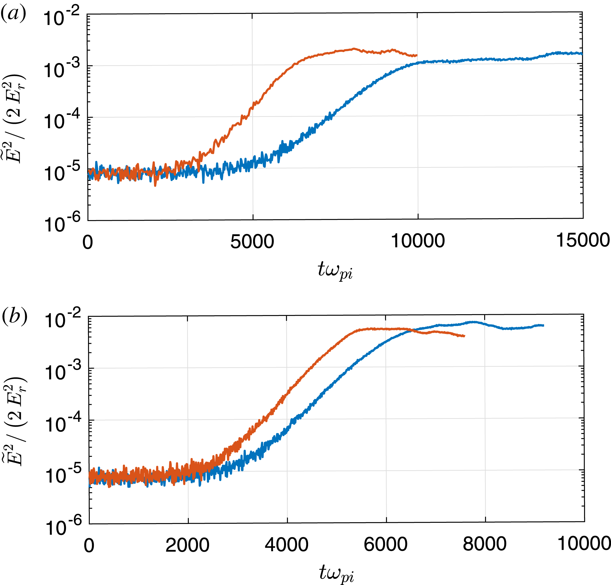
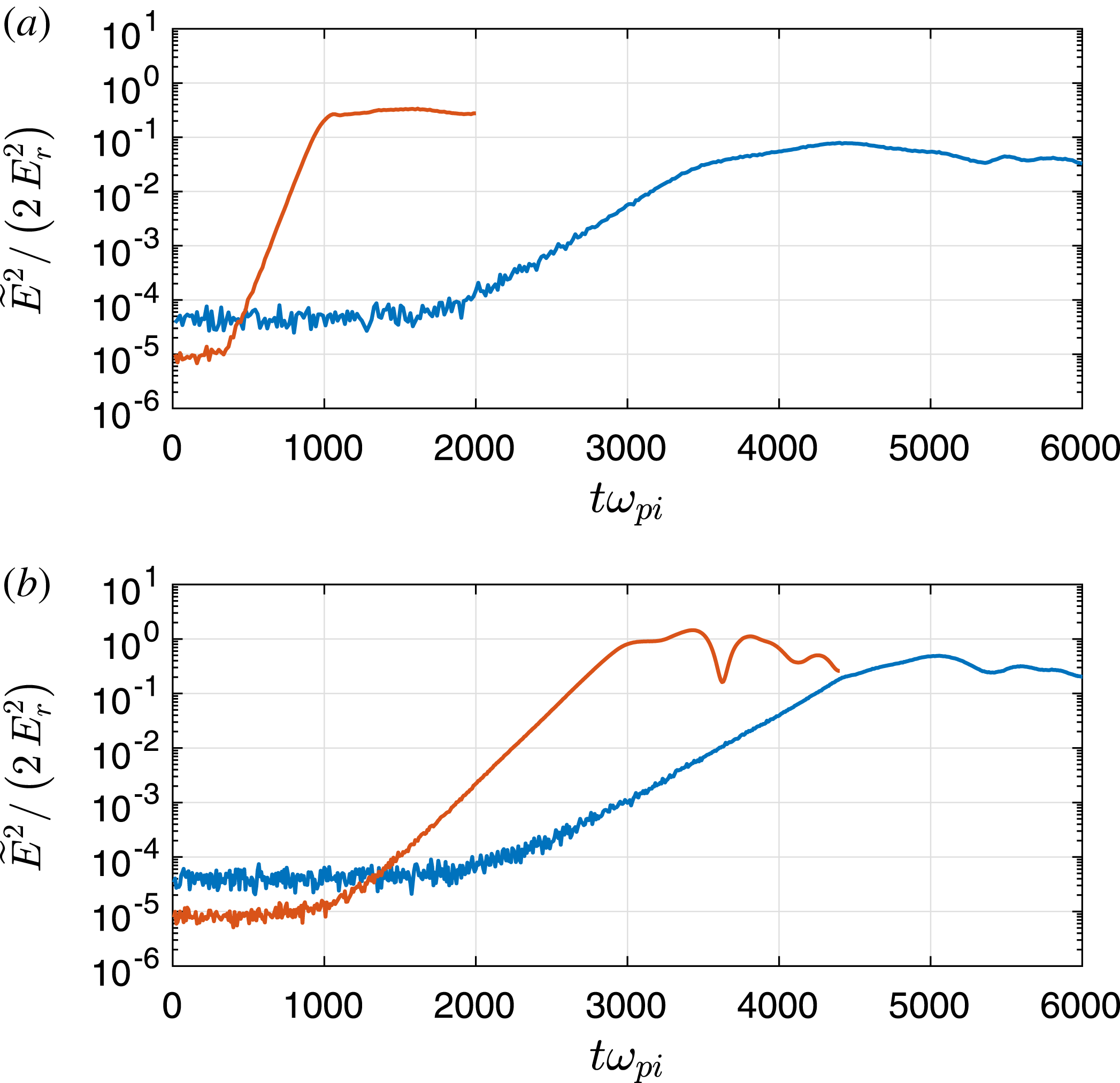
. Figure 2 shows the average wave electric field energy density as a function of time for this case, for two values of the ion collision rate, for both the non-Maxwellian and shifted-Maxwellian ion distributions. As can be seen, there is only a small difference in the maximum wave energy density in the simulations with non-Maxwellian versus shifted-Maxwellian ion distributions. In addition, the time scales for the growth phases appear similar, which appears consistent with the behaviour of the maximum growth rates for
 $M_{\text{th}}=1$
shown in figure 5 of Kählert (Reference Kählert2015).
Average wave electric field energy density as a function of time for Case I simulations, with (a)
 $\unicode[STIX]{x1D708}_{i}/\unicode[STIX]{x1D714}_{\text{pi}}=0.1$
and (b)
 $\unicode[STIX]{x1D708}_{i}/\unicode[STIX]{x1D714}_{\text{pi}}=0.5$
. The blue (red) curves correspond to the simulation with a non-Maxwellian (shifted-Maxwellian) ion velocity distribution at
 $t=0$
.

It can also be seen from figure 2 that the maximum wave electric field energy density is larger in the simulations with higher ion collision frequency. This trend has also been observed in previous simulations of dust acoustic instability in a collisional plasma (Winske & Rosenberg Reference Winske and Rosenberg1998; Winske Reference Winske2004). (The increase of wave electric field energy density with increasing collisionality of the driver particle species has also been observed in simulations of the ion acoustic instability (Sydora et al. Reference Sydora, Detering, Rozmus, Bychenkov, Brantov and Capjack2006)). The effect may be due to the de-trapping by collisions of ions that are trapped in the wave potentials, leading to the larger growth of waves. We will discuss this scenario in more detail in the next section.
Case II
Case II corresponds to an initial ion drift speed of
 $M_{\text{th}}=3$
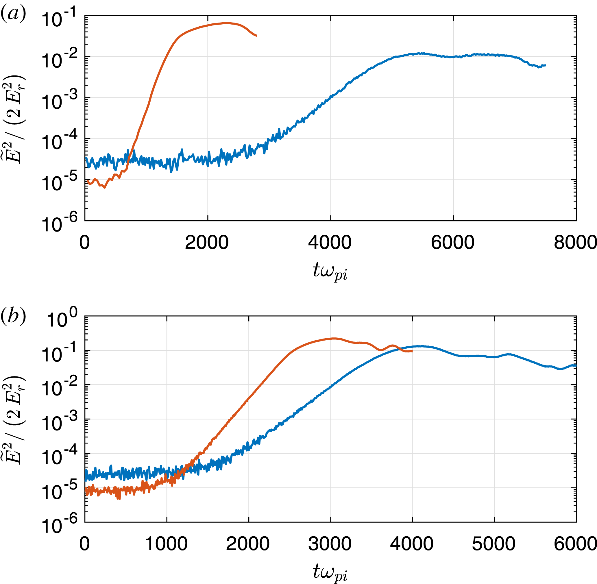
. Figure 3 shows the average wave electric field energy density as a function of time for both the non-Maxwellian and shifted-Maxwellian ion velocity distributions. As contrasted with figure 2, it can be seen that, for
 $\unicode[STIX]{x1D708}_{i}/\unicode[STIX]{x1D714}_{\text{pi}}=0.1$
, there is a significant difference in the maximum wave energy density for the two different ion distribution cases, where the maximum wave energy density is approximately 7–8 times larger in the simulation with shifted-Maxwellian ions. For the higher collision frequency
 $\unicode[STIX]{x1D708}_{i}/\unicode[STIX]{x1D714}_{\text{pi}}=0.5$
, the maximum wave energy density is comparable in both simulations, and larger than for the case with
 $\unicode[STIX]{x1D708}_{i}/\unicode[STIX]{x1D714}_{\text{pi}}=0.1$
.
Average wave electric field energy density as a function of time for Case II simulations, with (a)
 $\unicode[STIX]{x1D708}_{i}/\unicode[STIX]{x1D714}_{\text{pi}}=0.1$
and (b)
 $\unicode[STIX]{x1D708}_{i}/\unicode[STIX]{x1D714}_{\text{pi}}=0.5$
. The blue (red) curves correspond to the simulation with a non-Maxwellian (shifted-Maxwellian) ion velocity distribution at
 $t=0$
.

From figure 3, it can be seen that for the lower ion collision frequency,
 $\unicode[STIX]{x1D708}_{i}/\unicode[STIX]{x1D714}_{\text{pi}}=0.1$
, the roughly linear growth phase is approximately 3 times more rapid in the case with shifted-Maxwellian ions than for the case with non-Maxwellian ions. On the other hand, the time scale of the growth phase for the larger collision frequency,
 $\unicode[STIX]{x1D708}_{i}/\unicode[STIX]{x1D714}_{\text{pi}}=0.5$
is comparable for simulations with either non-Maxwellian or shifted-Maxwellian ion distributions. Both of these behaviours appear consistent with the behaviour of the maximum growth rates shown in figure 5 of Kählert (Reference Kählert2015).
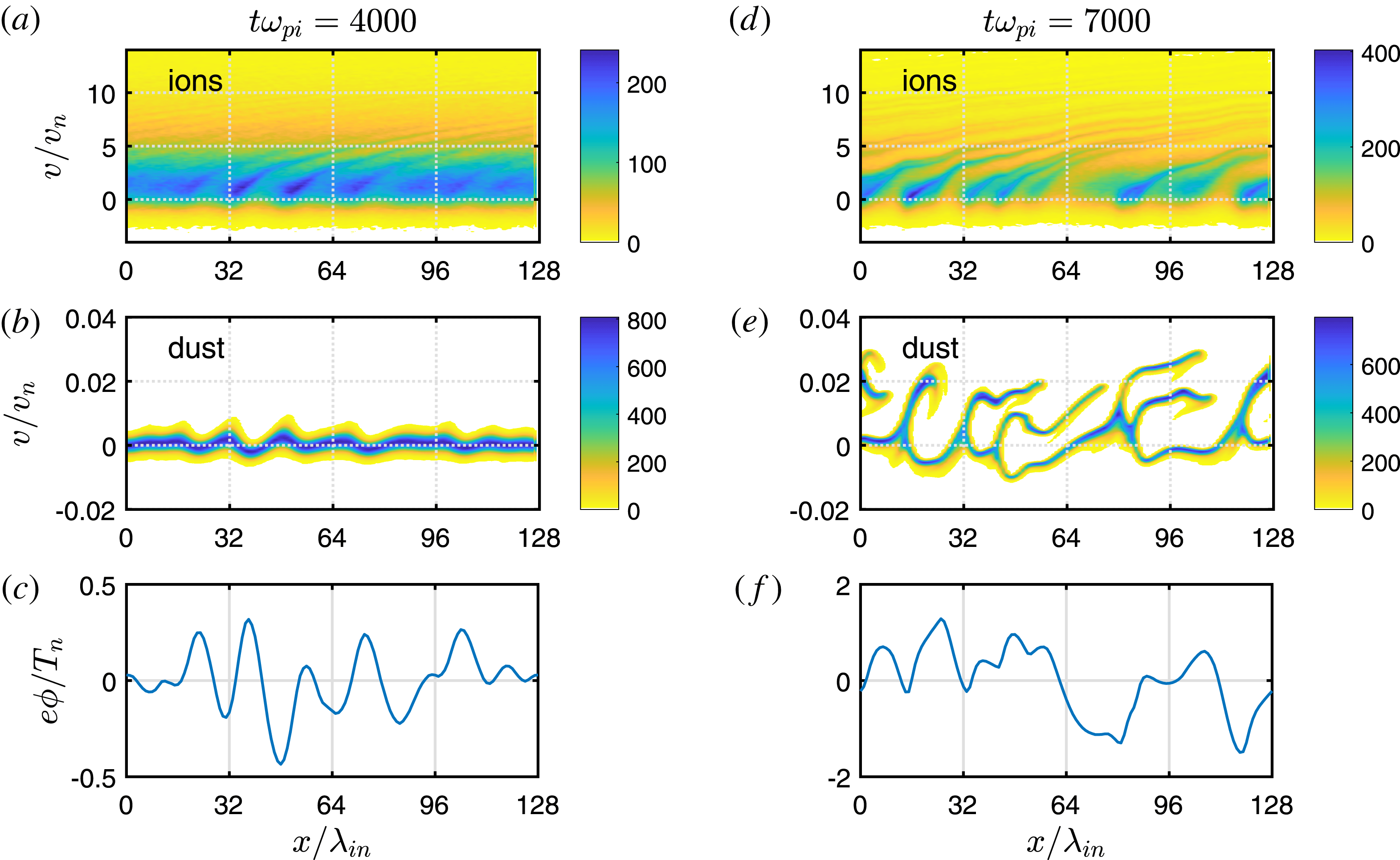
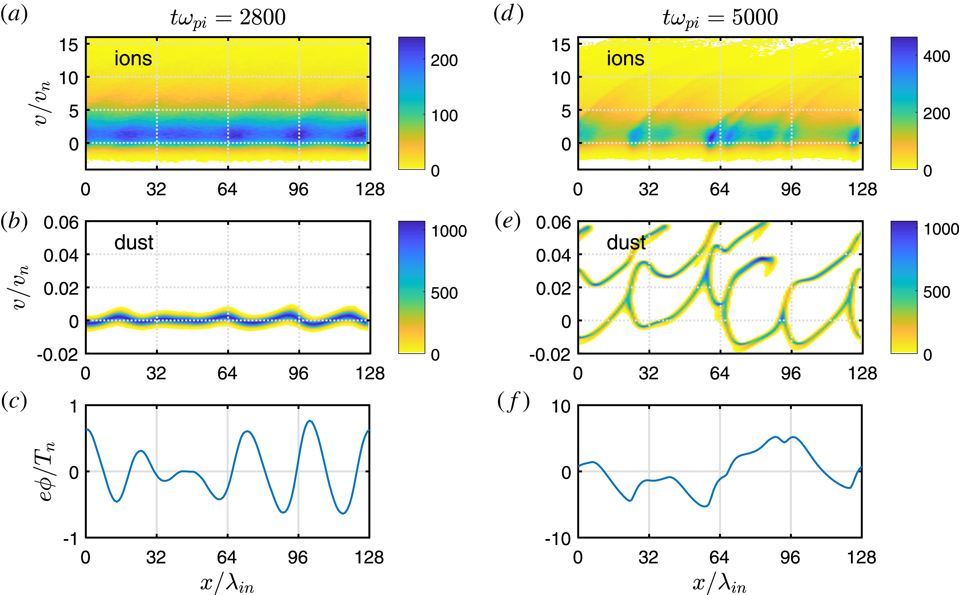
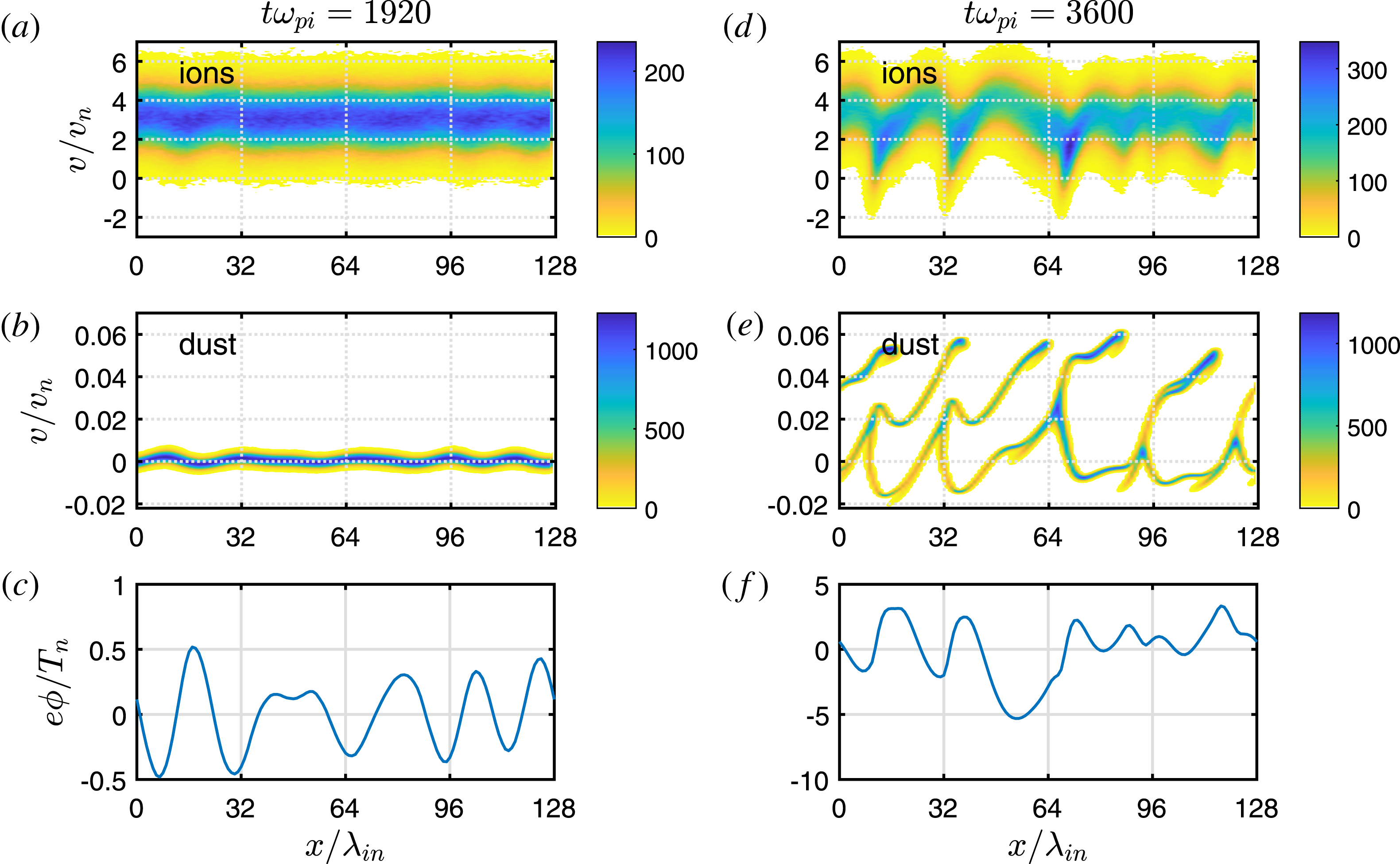
The panels in figures 4–7 show ion and dust phase space plots, along with the spatial structure of the wave electrostatic potential, at a time during the rapid growth phase, and at a later time in the nonlinear phase, for
 $\unicode[STIX]{x1D708}_{i}/\unicode[STIX]{x1D714}_{\text{pi}}=0.1$
with non-Maxwellian ions (figure 4) or shifted-Maxwellian ions (figure 5), and for
 $\unicode[STIX]{x1D708}_{i}/\unicode[STIX]{x1D714}_{\text{pi}}=0.5$
, with non-Maxwellian ions (figure 6) or shifted-Maxwellian ions (figure 7). The legend in these figures indicates the relative particle density. A number of trends can be seen from these panels that we discuss in the following.
Phase space plots and spatial structure of the wave potential for two different times in the Case II simulations with
 $\unicode[STIX]{x1D708}_{i}/\unicode[STIX]{x1D714}_{\text{pi}}=0.1$
and non-Maxwellian ions:
 $t\unicode[STIX]{x1D714}_{\text{pi}}=4000$
(a–c) and
 $t\unicode[STIX]{x1D714}_{\text{pi}}=7000$
(d–f). The ion phase space plots are shown in (a,d), the dust phase space plots in (b,e) and the wave potential in (c,f).

First we consider the simulations with
 $\unicode[STIX]{x1D708}_{i}/\unicode[STIX]{x1D714}_{\text{pi}}=0.1$
(figures 4 and 5). Counting the peaks of the wave potentials in the panels corresponding to the linear growth phase suggests that, roughly, the dominant wavelength for the simulation with non-Maxwellian ions is comparable to that for the simulation with shifted-Maxwellian ions. This is also consistent with a Fourier analysis of the potential (not shown). The ion phase space plot in figure 4(a) shows that there can be some localized regions of enhanced ion density at low velocities even in the linear growth phase for the case with non-Maxwellian ions. These ion phase space ‘bunches’ appear to be located spatially in the vicinity of the minima of the wave potential, and thus may be due to trapping in the waves. For the case with shifted-Maxwellian ions, there appears to be significantly less ion trapping in the linear phase shown in figure 5(a).
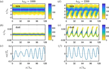
Same as figure 4, but with shifted-Maxwellian ions.

We suggest a possible explanation for the ion phase space behaviour described in the previous paragraph. The condition for trapping is (e.g. Winske Reference Winske2004)
 $$\begin{eqnarray}\displaystyle eZ\unicode[STIX]{x1D719}\sim \frac{m}{2}\left(\frac{\unicode[STIX]{x1D714}_{\text{max}}}{k_{\text{max}}}-U\right)^{2}, & & \displaystyle\end{eqnarray}$$
where
 $U$
is the mean velocity of the trapped species and
 $\unicode[STIX]{x1D714}_{\text{max}}/k_{\text{max}}$
is the phase speed of the maximally unstable wave. For the ions,
 $U$
is much larger than the phase speed of the dust wave, so we have
 $$\begin{eqnarray}\displaystyle \frac{e\unicode[STIX]{x1D719}}{T_{n}}\sim \frac{U^{2}}{2v_{n}^{2}}. & & \displaystyle\end{eqnarray}$$
In the simulation with shifted-Maxwellian ions, the ion distribution is peaked at the (mean) drift velocity
 $U_{i}\approx 3v_{n}$
, so (3.2) implies
 $e\unicode[STIX]{x1D719}/T_{n}\sim 4.5$
. As this value is not attained in the linear stage (see figure 5
c), so one would not expect much ion trapping, which seems consistent with the ion phase space plot in figure 5(a). On the other hand, in the simulation with non-Maxwellian ions, the velocity distribution is broader, peaking in the region
 $0\lesssim v_{x}/v_{n}\lesssim 2$
, with considerably more ions at lower speeds than the shifted-Maxwellian distribution (see figure 1). In this case, some trapping of low-energy ions might occur even in the linear phase. For example, taking
 $U\sim v_{n}$
, condition (3.2) implies
 $e\unicode[STIX]{x1D719}/T_{n}\sim 0.5$
, which could be attained in the linear stage (see figure 4
c). This is consistent with the ion phase space plot in figure 4(a), which seems to show some localized ion trapping. However, ion collisions can compete with trapping if the bounce frequency of an ion trapped in the wave
 $\unicode[STIX]{x1D708}_{b}\sim (ek_{\text{max}}^{2}\unicode[STIX]{x1D719}/m_{i})^{1/2}$
is comparable to
 $\unicode[STIX]{x1D708}_{i}$
(e.g. Quest et al.
Reference Quest, Rosenberg, Kercher and Dutreix2016) (see also Nishikawa & Wu Reference Nishikawa and Wu1969; Albright Reference Albright1974). This can be written as
 $$\begin{eqnarray}\displaystyle \frac{\unicode[STIX]{x1D708}_{b}}{\unicode[STIX]{x1D714}_{\text{pi}}}\sim k_{\text{max}}\unicode[STIX]{x1D706}_{\text{in}}\left(\frac{e\unicode[STIX]{x1D719}}{T_{n}}\right)^{1/2}\sim \frac{\unicode[STIX]{x1D708}_{i}}{\unicode[STIX]{x1D714}_{\text{pi}}}. & & \displaystyle\end{eqnarray}$$
Estimating
 $e\unicode[STIX]{x1D719}/T_{n}\sim 0.2$
in the linear phase from figure 4(c), we roughly estimate
 $\unicode[STIX]{x1D708}_{b}/\unicode[STIX]{x1D714}_{\text{pi}}\gtrsim \unicode[STIX]{x1D708}_{i}/\unicode[STIX]{x1D714}_{\text{pi}}$
, taking
 $k_{\text{max}}\unicode[STIX]{x1D706}_{\text{in}}\sim 2\unicode[STIX]{x03C0}7/128\sim 0.4$
. Thus collisions may play a role in de-trapping. However, in the case of charge-exchange collisions, each collision results in a slow ion, thus in effect adding ions to the low-energy region of the ion distribution which is more susceptible to trapping by the wave fields. This is in contrast to the case of ion–neutral collisions modelled with a Langevin operator; combined with the presence of the driver field, the resulting small angle scattering acts to maintain the shifted-Maxwellian ion distribution, and in the absence of wave fields does not result in particles shifting to lower velocities.
At later times in the simulation with non-Maxwellian ions, the low-energy, localized ion ‘bunches’ become more pronounced, as seen in figure 4(d). In addition, ions with higher energies appear to move on ballistic trajectories under the influence of the background driver electric field. The distance over which these higher-energy ions can move, approximately a mean free path
 ${\sim}v_{i}/\unicode[STIX]{x1D708}_{i}$
, can be large for the ions in the tail of the distribution. This behaviour can be contrasted with the ion phase space plots in the simulation with shifted-Maxwellian ions shown in figure 5(d), where at later times the ions velocities appear to shift to lower values and even negative values, reminiscent of plateau formation. This latter behaviour may be analogous to plateau formation in the electron distribution in the nonlinear phase of the Buneman instability (see e.g. Pavan, Yoon & Umeda Reference Pavan, Yoon and Umeda2011).
The dust phase space plots in figures 4(e) and 5(e) show that the dust gets heated by the waves in the nonlinear phase. We roughly estimate the condition for dust trapping from (3.1) by taking
 $U=0$
and assuming
 $k_{\text{max}}U_{i}\sim \unicode[STIX]{x1D714}_{\text{pi}}$
and
 $\unicode[STIX]{x1D714}_{\text{max}}\sim \unicode[STIX]{x1D714}_{\text{pd}}$
(see Rosenberg (Reference Rosenberg1996) for the shifted-Maxwellian case) to obtain
 $\unicode[STIX]{x1D714}_{\text{max}}/k_{\text{max}}\sim 3\unicode[STIX]{x1D706}_{\text{in}}\unicode[STIX]{x1D714}_{\text{pd}}$
, which yields
 $e\unicode[STIX]{x1D719}/T_{n}\sim (9/2)Z_{d}n_{n}/n_{i}\sim 1.8$
for the considered parameters. The wave potentials shown in figures 4(f) and 5(f) appear to be large enough for some dust trapping, which is consistent with the heating shown in the dust phase space plots.
Next we consider the simulations with
 $\unicode[STIX]{x1D708}_{i}/\unicode[STIX]{x1D714}_{\text{pi}}=0.5$
(figures 6 and 7). As discussed previously regarding figure 3, at this higher ion collision rate, the maximum wave energy densities are comparable for the simulations with the two different ion distributions, and are larger than the case with
 $\unicode[STIX]{x1D708}_{i}/\unicode[STIX]{x1D714}_{\text{pi}}=0.1$
. This may be because collisional effects tend to reduce ion trapping, so that the waves can grow to larger amplitude (see also Winske Reference Winske2004). The dominant wavelength in the linear phase also appears to be comparable in the two cases (roughly estimated by counting the peaks in
 $\unicode[STIX]{x1D719}$
in figures 6(c) and 7(c)), with longer wavelength than in the simulations with
 $\unicode[STIX]{x1D708}_{i}/\unicode[STIX]{x1D714}_{\text{pi}}=0.1$
.
Phase space plots and spatial structure of the wave potential for two different times in the Case II simulations with
 $\unicode[STIX]{x1D708}_{i}/\unicode[STIX]{x1D714}_{\text{pi}}=0.5$
and non-Maxwellian ions:
 $t\unicode[STIX]{x1D714}_{\text{pi}}=2800$
(a–c) and
 $t\unicode[STIX]{x1D714}_{\text{pi}}=5000$
(d–f). The ion phase space plots are shown in (a,d), the dust phase space plots in (b,e) and the wave potential in (c,f).

Same as figure 6, but with shifted-Maxwellian ions.

A difference between the two simulations for
 $\unicode[STIX]{x1D708}_{i}/\unicode[STIX]{x1D714}_{\text{pi}}=0.5$
appears to be in the ion phase space plots. Figure 6(a) shows the beginning of localized, low-energy ion bunches in the linear phase of the simulation with non-Maxwellian ions. As in the case with
 $\unicode[STIX]{x1D708}_{i}/\unicode[STIX]{x1D714}_{\text{pi}}=0.1$
, the wave potential in this phase may be large enough to trap ions with the non-Maxwellian distribution which has a peak at
 $v_{x}/v_{n}\sim 1{-}2$
. To estimate whether collisions could compete with trapping we use (3.3) with
 $k_{\text{max}}\unicode[STIX]{x1D706}_{\text{in}}\sim 2\unicode[STIX]{x03C0}5/128\sim 0.25$
and
 $e\unicode[STIX]{x1D719}/T_{n}\sim 0.5$
from figure 6(c) which yields
 $\unicode[STIX]{x1D708}_{b}/\unicode[STIX]{x1D714}_{\text{pi}}\sim 0.2<\unicode[STIX]{x1D708}_{i}/\unicode[STIX]{x1D714}_{\text{pi}}=0.5$
. Thus, collisions could compete with the apparent ion trapping in the linear phase for the non-Maxwellian ions.
At later times in the nonlinear phase, figure 6(d) shows that in the simulation with non-Maxwellian ions, the low-energy localized ion bunches become more pronounced. The higher-energy ions appear to move ballistically as in the case of
 $\unicode[STIX]{x1D708}_{i}/\unicode[STIX]{x1D714}_{\text{pi}}=0.1$
, but over a shorter distance due to the reduced mean free path at higher collision rate. In the simulation with shifted-Maxwellian ions, the phase space plot at later times in figure 7(d) shows that the ion energy moves to lower values and even negative values, again reminiscent of plateau formation.
Case III
Case III corresponds to an initial ion drift speed of
 $M_{\text{th}}=6$
. Figure 8 shows the average wave electric field energy density as a function of time for both the non-Maxwellian and shifted-Maxwellian ion velocity distributions. As in the Case II simulations, for
 $\unicode[STIX]{x1D708}_{i}/\unicode[STIX]{x1D714}_{\text{pi}}=0.1$
there is a significant difference in the maximum wave energy density for the two different ion distribution cases, with the maximum wave energy density approximately 3–4 times larger in the simulation with shifted-Maxwellian ions. For the higher collision frequency
 $\unicode[STIX]{x1D708}_{i}/\unicode[STIX]{x1D714}_{\text{pi}}=0.5$
, the maximum wave energy density is comparable in both simulations, and larger than for the case with
 $\unicode[STIX]{x1D708}_{i}/\unicode[STIX]{x1D714}_{\text{pi}}=0.1$
. It can also be seen from figure 8 that for
 $\unicode[STIX]{x1D708}_{i}/\unicode[STIX]{x1D714}_{\text{pi}}=0.1$
, the roughly linear growth phase is approximately 4 times more rapid in the case with shifted-Maxwellian ions than in the case with non-Maxwellian ions. For
 $\unicode[STIX]{x1D708}_{i}/\unicode[STIX]{x1D714}_{\text{pi}}=0.5$
, the growth phase is approximately 1.5 times more rapid in the simulation with shifted-Maxwellian ions compared with the simulation with non-Maxwellian ions. These latter two results appear consistent with the behaviour of the maximum growth rates shown in figure 5 of Kählert (Reference Kählert2015).
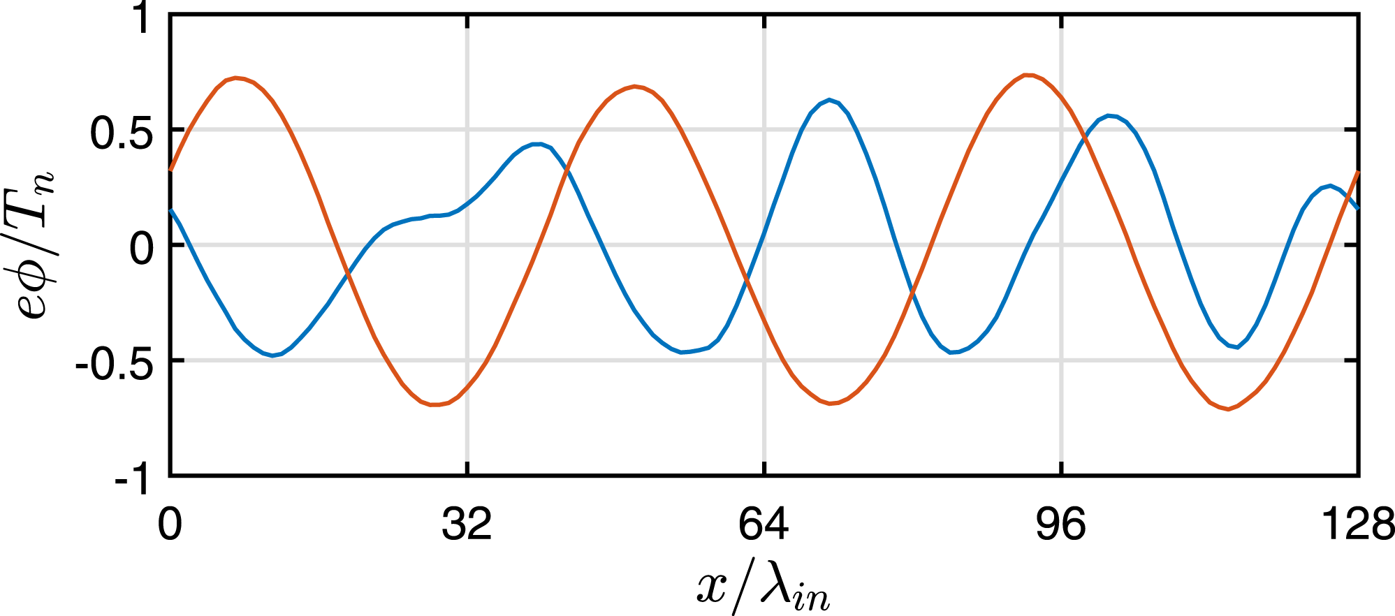
It is also of interest to estimate the dominant wavelength in the linear growth phase for the two simulations. Figure 9 shows a plot of the wave potential structure in the linear growth phase for the case where
 $\unicode[STIX]{x1D708}_{i}/\unicode[STIX]{x1D714}_{\text{pi}}=0.1$
. It appears that the dominant wavelength in the simulation with non-Maxwellian ions is smaller by a factor of approximately 3/4 than in the simulation with shifted-Maxwellian ions. This appears reasonably consistent with the behaviour of the wavenumber at maximal growth shown in figure 4 of Kählert (Reference Kählert2015).
Average wave electric field energy density as a function of time for Case III simulations, with (a)
 $\unicode[STIX]{x1D708}_{i}/\unicode[STIX]{x1D714}_{\text{pi}}=0.1$
and (b)
 $\unicode[STIX]{x1D708}_{i}/\unicode[STIX]{x1D714}_{\text{pi}}=0.5$
. The blue (red) curves correspond to the simulation with a non-Maxwellian (shifted-Maxwellian) ion velocity distribution at
 $t=0$
.

Spatial structure of the wave potential in the linear phase for the Case III simulation with
 $\unicode[STIX]{x1D708}_{i}/\unicode[STIX]{x1D714}_{\text{pi}}=0.1$
. The blue curve is for the simulation with non-Maxwellian ions, at time
 $t\unicode[STIX]{x1D714}_{\text{pi}}=2800$
, and the red curve is for the simulation with shifted-Maxwellian ions at time
 $t\unicode[STIX]{x1D714}_{\text{pi}}=704$
.

4 Summary and discussion
We presented 1-D PIC simulations of the nonlinear development of the ion–dust streaming instability using two different ion velocity distributions: a non-Maxwellian and a shifted Maxwellian. In both cases, in our model plasma the ions are subject to a uniform background electric field and undergo collisions with neutrals. In the non-Maxwellian case, the ions undergo charge-exchange collisions modelled with a constant collision frequency. In the shifted-Maxwellian case, the ion collisions are modelled by a Langevin operator. We showed results for several values of the ion thermal Mach number
 $M_{\text{th}}=U_{i}/v_{n}=1,3,6$
and for both a lower and a higher ion collision rate,
 $\unicode[STIX]{x1D708}_{i}/\unicode[STIX]{x1D714}_{\text{pi}}=0.1$
and 0.5. The results for the simulations with non-Maxwellian and shifted-Maxwellian ion distributions were compared.
For
 $M_{\text{th}}=1$
, it was found that the maximum wave energy and instability growth times were similar for the simulations with non-Maxwellian and shifted-Maxwellian ions. However, for larger
 $M_{\text{th}}$
it was found that the maximum wave energy density is smaller in the simulations with non-Maxwellian ions, particularly for the lower ion collision rate. In addition, it appears that in the simulations with non-Maxwellian ions and larger
 $M_{\text{th}}$
, the ions can become trapped by the waves in localized ion ‘bunches’ even in the linear phase. This may be due to the nature of the non-Maxwellian ion distribution which has a peak in the region
 $v_{x}/v_{n}\sim 1{-}2$
even for larger
 $M_{\text{th}}$
, along with a high-energy tail. Thus, because there are more low-energy ions than in the shifted-Maxwellian distribution, the ions can be more easily trapped by waves. It should be noted that even though the ions appear to be spatially bunched in the linear phase, there is still growth of the instability. This may be because the form of the ion velocity distribution may be similar to its initial distribution over at least a wavelength. It was also found that, in the simulations with non-Maxwellian ions, the instability growth time was longer and the dominant wavelength was shorter, for larger
 $M_{\text{th}}$
and lower ion collision rate. This appears to be consistent with the linear theory results of Kählert (Reference Kählert2015). At the higher collision rate, the results of the simulations appear to be more similar for the two types of ion distributions.
Future work will include the effect of dust–neutral collisions, which tend to thermalize the dust and can thus lower dust heating by the waves. We also intend to use a different, more realistic model for charge-exchange collisions based on a constant collision cross-section instead of a constant collision frequency. Lampe et al. (Reference Lampe, Rocker, Joyce, Zhdanov, Ivlev and Morfill2012) have shown that in this case, the ion distribution obtained balancing collisional drag with the electric force in a uniform electric field has a half-Gaussian form rather than an exponential tail for large
 $M_{\text{th}}$
. This is because the collision rate, which is proportional to the ion speed, is larger for the high-energy ions, resulting in more low-energy ions than for the constant collision frequency model. We speculate that this might further enhance the effect of ion trapping by the waves in the nonlinear phase of the ion–dust streaming instability, perhaps leading to a lower maximum wave energy.
A limitation of the 1-D simulations is that they do not account for the possibility of dust density waves that propagate at an oblique angle with respect to the ion flow, which was observed and discussed by Piel et al. (Reference Piel, Klindworth, Arp, Melzer and Wolter2006). The consideration of this scenario would require a 2-D simulation, which could also allow for the possible mixing of excited modes in the nonlinear phase.
Acknowledgement
This work was partially supported by NSF and NASA.