2.1 Fuzzy cluster method

A novel approach is proposed which identifies the internal interfacial layers by grouping contiguous and non-contiguous zones according to common flow features. Here, we consider flow fields from an instantaneous snapshot of a large-eddy simulation (LES), direct numerical simulation (DNS) or particle image velocimetry (PIV, either planar or volumetric) database. The entirety of the flow data within a given snapshot forms a sequence of observations, $\unicode[STIX]{x1D731}=\{\unicode[STIX]{x1D6F7}^{m}\}_{m=1}^{N}$ , where $N$ represents the total number of grid points in the snapshot and $\unicode[STIX]{x1D6F7}$ a scalar quantity such as pressure or velocity component (Friedman, Hastie & Tibshirani Reference Friedman, Hastie and Tibshirani2001). As the clustering is done on the streamwise velocity in the current paper, we replace $\unicode[STIX]{x1D6F7}$ with $U$ to simplify the notation. The cluster analysis aims at grouping the observations $\{U^{m}\}_{m=1}^{N}$ into $K$ clusters, $\unicode[STIX]{x1D6F1}_{k}$ (with $k=1,\ldots ,K$ ), based on their similar streamwise velocity. To quantify similar flow features, a distance metric between two observations is defined as $D_{mn}=|U^{m}-U^{n}|$ , where the norm is in the Euclidean space. We adopt an FCM (Dunn Reference Dunn1973; Bezdek Reference Bezdek1981) in which a membership coefficient $u_{mk}$ represents the probability of the observation $U^{m}$ belonging to cluster $\unicode[STIX]{x1D6F1}_{k}$ . Based on this definition, $\sum _{k=1}^{K}u_{mk}=1$ . We define $c^{k}$ as the centroid of cluster $k$ , accordingly, it represents the characteristic velocity of the cluster. It corresponds to the average of all observations with the membership function $u_{mk}$ :

(2.1) $$\begin{eqnarray}\displaystyle c^{k}=\frac{\displaystyle \mathop{\sum }_{m=1}^{N}(u_{mk})^{p}U^{m}}{\displaystyle \mathop{\sum }_{m=1}^{N}(u_{mk})^{p}}, & & \displaystyle\end{eqnarray}$$

where $p\in [1,\infty )$ is the fuzziness parameter in FCM and is usually set to 2 in practice (Pal & Bezdek Reference Pal and Bezdek1995). The cluster centroids form a centroid vector $\boldsymbol{c}=(c^{1},\ldots ,c^{K})$ . The cluster centroid represents a characteristic velocity of each cluster and, as for the modal velocity in the histogram method, represents the characteristic velocity of each zone. Once $\boldsymbol{c}$ and $u_{mk}$ are determined, the variance can be defined as an object function

(2.2) $$\begin{eqnarray}\displaystyle J_{p}(\boldsymbol{U},\boldsymbol{c})=\mathop{\sum }_{m=1}^{N}\mathop{\sum }_{k=1}^{K}(u_{mk})^{p}(D_{mk})^{2}. & & \displaystyle\end{eqnarray}$$

The optimal $\boldsymbol{c}$ is determined by the minimization of the objective function via the standard Lagrange multiplier method. As a result, the FCM is a bootstrapping algorithm which is summarized as follows:

1. (1) initialize the membership coefficient $u_{mk}$ for each observation;

2. (2) compute the centroid of the clusters $c^{k}$ with equation (2.1);

3. (3) recompute the membership coefficient using the new $c^{k}$

   (2.3) $$\begin{eqnarray}\displaystyle u_{mk}=\left(\mathop{\sum }_{j=1}^{K}(D_{mk}/D_{mj})^{2/(p-1)}\right)^{-1}; & & \displaystyle\end{eqnarray}$$

4. (4) execute steps 2 and 3 iteratively until $|\boldsymbol{c}-\boldsymbol{c}_{\mathbf{0}}|\leqslant \unicode[STIX]{x1D716}$ , where $\unicode[STIX]{x1D716}$ is a pre-determined error threshold and $\boldsymbol{c}_{\mathbf{0}}$ is the centroid vector in the previous iteration.

Once converged, we assign the observation $U^{m}$ to $\unicode[STIX]{x1D6F1}_{k}$ with the highest membership $I_{m}=\text{arg}\,\text{max}_{k}(u_{mk})$ . Although it is reported that FCM can be sensitive to initial $u_{mk}$ (Pham, Xu & Prince Reference Pham, Xu and Prince2000), the present results are shown to be robust and invariant to the initialization. Naturally, the FCM algorithm requires a user-defined number of clusters $K$ , and various approaches to determine the optimal $K$ are possible. For example, Bezdek (Reference Bezdek1974) defined a partition coefficient to measure the ‘overlap’ between clusters and $K$ is selected when the partition coefficient reaches a minimum. In the following section, we propose an algorithm, based on a kernel density estimation (KDE) approach, to automatically select the appropriate number of zones for a given dataset. The interface identification code and the method to identify the number of zones – both written in Python – as well as all the datasets used are freely accessible online.

2.2 Selection of the number of IILs

The clustering approach rests on the understanding that we have an a priori knowledge of the number of clusters or IILs in a given flow. At low Reynolds number, the number of internal zones can be inferred from a physical understanding of the various regions within wall-bounded turbulent flow. This simplistic approach breaks down when faced with higher-Reynolds-number wall-bounded turbulent flows for which the number of zones is dependent on the Reynolds number (de Silva et al. Reference de Silva, Hutchins and Marusic2016). For this reason, we propose an alternative clustering approach that automatically determines the optimal number of zones based on the same streamwise velocity parameter as the FCM. The approach, which rests on a KDE algorithm, does suffer from some of the same shortcomings as the histogram-based approach (requires an adequate selection of domain length, inability to account for near-wall grid stretching etc.); in the current implementation it is only used to determine the number of zones, and by extension, the number of IILs.

Kernel density estimation is a statistical method which is used to estimate the underlying probability density function from a set of sampled data. A kernel is placed at each observation and the results are summed to produce a smooth probability density function which accounts for the density of the observed samples. Two important parameters of the KDE are the shape of the kernel and the bandwidth, which acts as a smoothing parameter. Although there are a variety of possible kernels which can be used, the bandwidth has a much more significant effect on the results of the KDE. In our analysis, we use a Gaussian kernel; more information on the density estimation can be found in Silverman (Reference Silverman1998). Based on a minimization of the mean integrated squared error, the optimal bandwidth $h$ for a normal kernel is calculated as (Scott Reference Scott1992)

(2.4) $$\begin{eqnarray}\displaystyle h=\unicode[STIX]{x1D70E}(4/3)^{1/5}n^{-1/5}, & & \displaystyle\end{eqnarray}$$

where $\unicode[STIX]{x1D70E}$ is the standard deviation and $n$ is the number of observations.

Figure 1.

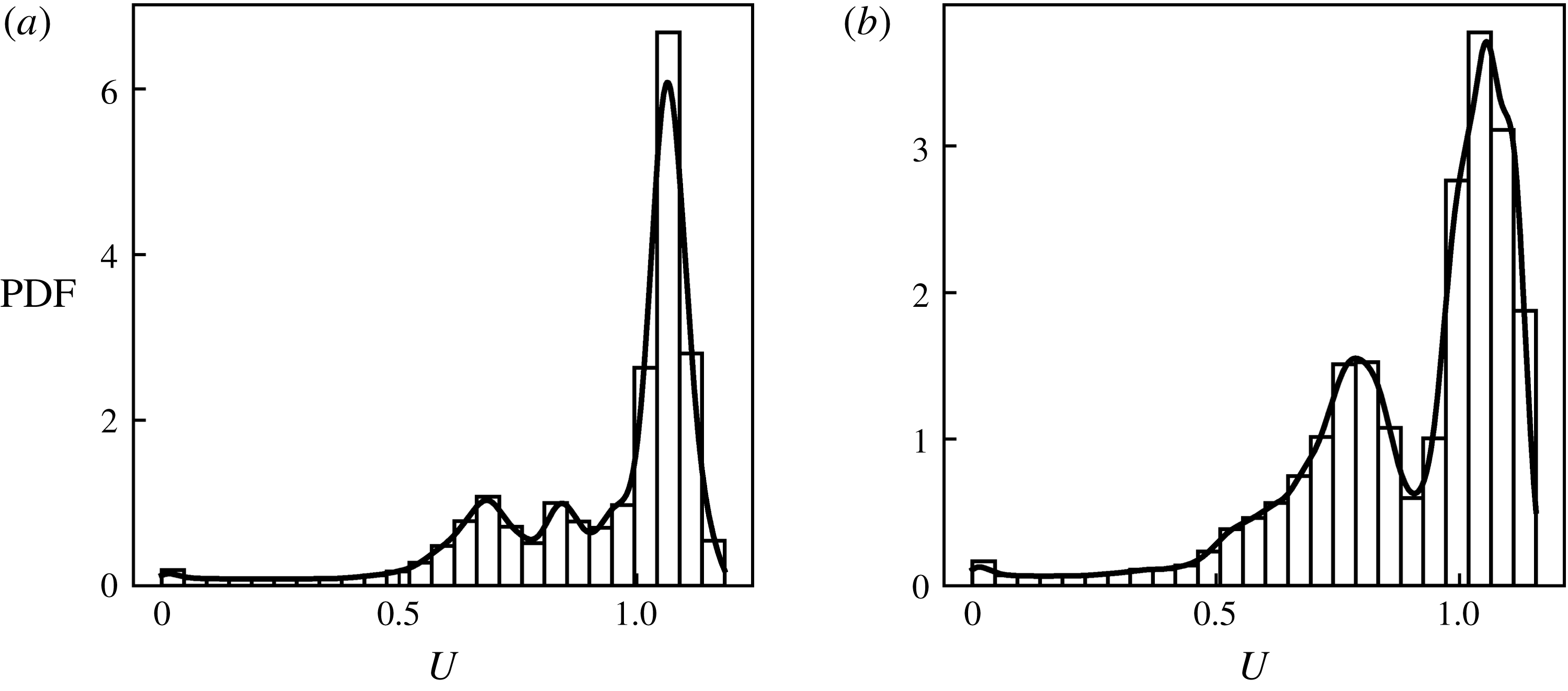
Kernel density estimation at two different streamwise locations of DNS channel flow data (Lee & Moser Reference Lee and Moser2015).

An example of a KDE applied over the same window size at two different streamwise locations of DNS channel flow data from Lee & Moser (Reference Lee and Moser2015) is shown in figure 1. The automatic bandwidth determination allows for an accurate identification of the number of internal zones. Similar to the histogram method, the KDE is conducted on a slice-by-slice basis. Although the number of peaks is defined without user input, the clustering would subsequently have to be performed on the thin region where the predicted number of zones is valid.

To group the data, a clustering approach based on KDE called mean shift clustering can be applied. Similar to KDE, the correct bandwidth selection has been studied and there are many recommendations, eliminating the need for the user to arbitrarily input a bandwidth. Despite promising results on PIV data, which has well-defined peaks, the mean shift clustering approach misidentifies the peaks in the presence of the smaller grid sizes near the wall in DNS results. The newly proposed fuzzy clustering method, presented in the previous subsection, does not have the same limitations.

Although the selection of the number of zones is a key input to the FCM, the correct identification of IIL is nonetheless possible if the selected number of zones is slightly incorrect (say $\pm$ 1), see § 4, which discusses the sensitivity and robustness of our method to the selection of the number of zones. In other words, if a flow is composed of three internal zones (two IILs), the same two IILs will be identified by the method if we wrongly input three IILs. This robustness assures a correct identification of the dynamically significant parts of the flow; as the proposed method does not require any user input (other than the velocity data), it provides a systematic approach to estimate the number of zones in a given database.

3.1 Experimental and numerical databases

Three publicly accessible turbulent flow databases – one experimental (PIV), two numerical (DNS) – are used for the validation of the proposed method (a fourth turbulent channel flow DNS at $Re_{\unicode[STIX]{x1D70F}}=750$ , on a small domain, was used to compute the average number of UMZs). Combined with our online accessible cluster algorithm (https://github.com/mxyao/Interfacial_Layer_Clustering), this assures a repeatable, transparent and generalizable assessment of our approach. First, we compare our cluster identification method against Adrian et al. (Reference Adrian, Meinhart and Tomkins2000)’s histogram-based approach by examining the planar PIV dataset of a turbulent boundary layer by Tomkins (Reference Tomkins1997). Second, the organization and conditional sampling of the IILs are analysed using two snapshots of the incompressible channel flow DNS by Del Álamo et al. (Reference Del Álamo, Jiménez, Zandonade and Moser2004) and two snapshot by Lee & Moser (Reference Lee and Moser2015). The friction velocity Reynolds number of the boundary layer (where $h$ is the boundary layer thickness) is $Re_{\unicode[STIX]{x1D70F}}=u_{\unicode[STIX]{x1D70F}}h/\unicode[STIX]{x1D708}=2216$ . The snapshots of the channel flow (where now $h$ is the channel half-height) are at 550, 950 (Del Álamo et al. 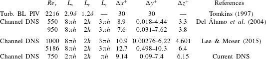Reference Del Álamo, Jiménez, Zandonade and Moser2004) and 1000, 5186 (Lee & Moser Reference Lee and Moser2015). The extent of the spatial domain and grid resolution of the datasets are summarized in table 1; further details can be found in the corresponding references.

Table 1.

Spatial domain and grid resolution of the boundary layer PIV measurements and the channel flow simulations. Note the ‘Current DNS’ is only used to estimate the number of UMZs in the following sections and not for the primary analysis.

3.2 Internal interface in the turbulent boundary layer

We first compare the IIL identification using the histogram and clustering approaches on the planar PIV data of a turbulent boundary layer. The algorithm proposed by de Silva et al. (Reference de Silva, Hutchins and Marusic2016) was used to identify the modal velocity of the UMZs based on the histogram peaks of the streamwise velocity. Two key features of de Silva et al. (Reference de Silva, Hutchins and Marusic2016)’s approach are: (1) the vector field above the TNTI and below $y^{+}=100$ is excluded from the histogram; (2) the histogram is constructed on a constrained domain of $L_{x}^{+}=2000$ . These imposed constraints on the histogram calculation are well reported in the literature. The removal of the near-wall and irrotational flow regions is needed to clearly observe multiple peaks in the histogram distribution, otherwise skewed modal velocities and/or additional peaks are observed. Furthermore, previous PIV studies on IILs (de Silva et al. Reference de Silva, Philip, Hutchins and Marusic2017) only cover a limited field of view (typically $2h$ ), primarily due to the ambiguity of the histogram-based method over a large spatial extent despite that IILs have been shown to correlate with very large-scale motion (VLSM) having a streamwise length proportional to $h$ (Adrian et al. Reference Adrian, Meinhart and Tomkins2000). Although the footprints of these VLSM are expected to be seen in the IIL, the limited field of view renders the detailed study of the interaction of these structures with the interfacial layers more difficult.

Figure 2.

(a) Comparison of the following interfacial layer identification algorithms on a turbulent boundary layer PIV frame: cluster-based algorithm (solid black lines), histogram-based IIL (dashed red line) and threshold-based TNTI (solid green line). The approach by de Silva et al. (Reference de Silva, Hutchins and Marusic2016) is used for the IIL detection. For the TNTI, a threshold on the local turbulent kinetic energy is used as proposed by Chauhan et al. (Reference Chauhan, Philip, de Silva, Hutchins and Marusic2014). The magnitude of the local spanwise vorticity is overlaid (minimum threshold on the non-dimensionalized vorticity magnitude is set to $10^{-4}U_{\infty }/\unicode[STIX]{x1D6FF}$ to highlight the vorticity concentration). (b) Instantaneous streamwise velocity profile (solid line) at $x/\unicode[STIX]{x1D6FF}=2.2$ (shown as a dashed vertical line in a) and mean velocity computed over the PIV frame (dashed blue line). Two randomly selected instantaneous streamwise velocity profiles are overlaid (dots). (c) Histogram of streamwise velocity based on streamwise domain length of $L_{x}^{+}=2000$ (bins), 4000 (dashed line) and 6000 (dashed-dotted line). (d) Cluster membership function, $u_{mk}$ , for zones 1, 2, 3 and FS. (e) Cluster centroid in all available PIV frames (41 in total) using FCM, zone 1 (◂), zone 2 (▸), zone 3 (●) and zone FS (▴).

The proposed clustering algorithm overcomes the above-noted limitations of the histogram-based approach. The FCM only requires the a priori knowledge of the number of UMZs. The KDE algorithm, described in § 2.2, correctly identifies four UMZs without the need of any user input. The identified zones have a direct physical representation in this flow. Near the wall, in the viscous sublayer, the viscosity effects dominate the dynamics and the length scales are proportional to $\unicode[STIX]{x1D708}/u_{\unicode[STIX]{x1D70F}}$ (zone 1). In zone 2, the flow is still influenced by the near-wall turbulence and inner wall scalings but the relative importance of the viscosity is reduced; this usually corresponds to the logarithmic region in the mean velocity profile. At the outer edge of the boundary layer (zone 3), the velocity profile is defined by outer scaling parameters, typically $\unicode[STIX]{x1D6FF}$ . Finally, the free-stream region of the boundary layer is non-turbulent and irrotational (zone 4 or FS). We note that the TNTI is identified at the interface between zones 3 and 4. Although the threshold-based TNTI identification methods are simple and straightforward, the cluster algorithm implicitly delineates this interface. The present cluster method can be used for TNTI identification when, for example, coarse experimental data at the outer boundary layer edge limit the ability to compute the local vorticity needed for the thresholding identification.

The direct comparison of histogram-based and cluster interface identification approaches is presented in figure 2(a), which corresponds to the PIV frame in Adrian et al. (Reference Adrian, Meinhart and Tomkins2000) (figure 19 in their paper). The streamwise velocity histogram has a local minimum at $U/U_{\infty }=0.8$ (when $L_{x}^{+}=2000$ ), see figure 2(c), which corresponds to the IIL delineating UMZs. In the cluster-based approach, we include all velocity vectors in the PIV frame and obtain the same interfaces (figure 2 a) and modal velocities (figure 2 c,d). The inspection of the instantaneous streamwise velocity profile at one $x/\unicode[STIX]{x1D6FF}$ location in figure 2(b) reveals a step-like change at the identified interfacial layers; similar step-like shifts are observed at the interfaces of other streamwise locations (not shown). As the IILs are conceptually thought to represent thin shear layers (Meinhart & Adrian Reference Meinhart and Adrian1995), we note a vorticity concentration in their vicinity (figure 2 a); the vorticity is observed at all of the three interfacial layers separating the four zones of the flow.

As noted by de Silva et al. (Reference de Silva, Hutchins and Marusic2016), the histogram-based IIL identification method is sensitive to the streamwise domain under consideration. By increasing the domain length from $L_{x}^{+}=2000$ to 4000, a third peak emerges in the histogram, see figure 2(c); this additional peak vanishes when the domain length is extended to $L_{x}^{+}=6000$ . Additionally, by considering the data points near the wall ( $y^{+}<100$ ) or in the free stream, the streamwise velocity histogram cannot uniquely identify the IIL on this dataset. In view of these constraints and limitations of the histogram method, the unambiguous identification of histogram peaks is only successful in approximately half of the PIV frames in the database (41 planar PIV frames are available). In many frames, clear modal peaks cannot be deciphered. However, hairpin structures and vortex packets can be observed in most frames. If we accept that UMZs are the result of these structures, UMZs and IILs should exist even when the histogram method fails. The modal velocities computed from the cluster-based method show an expected frame-to-frame variation but a high consistency, especially for zones 3 and FS, is noted among all PIV frames as shown figure 2(e). The lower resolution near the wall may account for the relatively higher variation in modal velocities of zones 1 and 2.

3.3 Interfacial layer in a turbulent channel flow

As shown in the previous subsection, the TNTI and IILs are unambiguously identified with a robust and repeatable cluster algorithm in a turbulent boundary layer. The interfaces obtained by clustering match those from the histogram (IIL) and turbulence threshold (TNTI) methods while overcoming many of the limitations of these classical approaches. Despite their three-dimensional nature, the ILLs have historically been identified from two-dimensional, experimental data. Unlike the TNTI identification which is trivially extended to three dimensions (Bisset et al. Reference Bisset, Hunt and Rogers2002; Hickey, Hussain & Wu Reference Hickey, Hussain and Wu2013; Borrell & Jiménez Reference Borrell and Jiménez2016), a surface IIL identification on volumetric data suffers from conceptual and practical limitations when using a histogram-based approach. As highlighted by Kwon et al. (Reference Kwon, Philip, de Silva, Hutchins and Monty2014) (figure 3f), the modal velocity peaks (used to identify the UMZs) are not detected in the streamwise velocity histogram in the three-dimensional channel flow. Only the very prominent modal velocity of the quiescent core is observed. Although the velocity histogram helps in the identification of the quiescent core, the detection of interfacial layers is impeded. Additionally, if we consider all numerical simulations, the local grid refinement near the wall gives rise to an artificial peak in the histogram due to a larger cell count of near-wall, lower-velocity points. The current cluster-based approach can be extended to unambiguously identify these three-dimensional, internal interfacial surfaces from numerical databases. In this section, we apply the cluster algorithm to three-dimensional, incompressible channel flow DNS data. First, we relate the number of UMZs to the Reynolds number of the flow (§ 3.3.1), then we compute the statistical features of the IILs (§ 3.3.2) and, finally, relate the geometric properties of the IIL to the large-scale organized motion in the channel flow (§ 3.3.3).

3.3.1 Number of UMZs

Unlike the turbulent boundary layer, which is typically bounded by an irrotational, free-stream region, the turbulent channel flow is fully turbulent. Based on this, we assume that a typical low-Reynolds-number channel flow consists of three zones: a viscous-dominated near-wall region (zone 1), a wall-turbulence-dominated region (zone 2) and an outer-scale-dominated region (zone 3). Zone 3 can also be called the ‘quiescent core’ although the exact definition used here differs somewhat from Kwon et al. (Reference Kwon, Philip, de Silva, Hutchins and Monty2014). This zonal delineation is supported by the results of the automatic KDE-based algorithm to determine the number of zones which is presented in § 2 for the low-Reynolds-number cases.

For high-Reynolds-number flows, the interfacial layers have thus far only been investigated using experimental data. The difficulty in obtaining near-wall experimental data with a sufficient spatial and temporal resolution over a large, three-dimensional field means that analysis of these IILs has been limited. Furthermore, existing histogram-based approaches are ill-suited for use on non-homogeneous grid spacing, as the grid refinement artificially affects the probability distribution of the streamwise velocity. Here we study IILs in the turbulent channel flow by Lee & Moser (Reference Lee and Moser2015) which is computed up to $Re_{\unicode[STIX]{x1D70F}}\approx 5200$ using a Fourier–Galerkin pseudo-spectral method in the streamwise and spanwise directions and a B-spline collocation method in the wall-normal direction. The details of the resolution are provided in table 1 and further information can be found in Lee & Moser (Reference Lee and Moser2015).

Uniform momentum zones are defined as regions of uniform streamwise velocity typically found within the logarithmic region of the turbulent boundary layer (Meinhart & Adrian Reference Meinhart and Adrian1995; de Silva et al. Reference de Silva, Hutchins and Marusic2016). When the full range of data in our method is used, we identify an IIL very close to the wall which bounds the viscous-dominated near-wall region (zone 1). However, this zone is inconsistent with the definition of a UMZ, which is typically found in the outer regions of the boundary layer. As such, in our analysis of UMZs, we do not consider this very near-wall zone to be a UMZ but it is nonetheless a delineated zone. For example, as we can see from figure 1, a small peak emerges at $U\approx 0$ ; this peak is not counted in the average number of UMZ computations below.

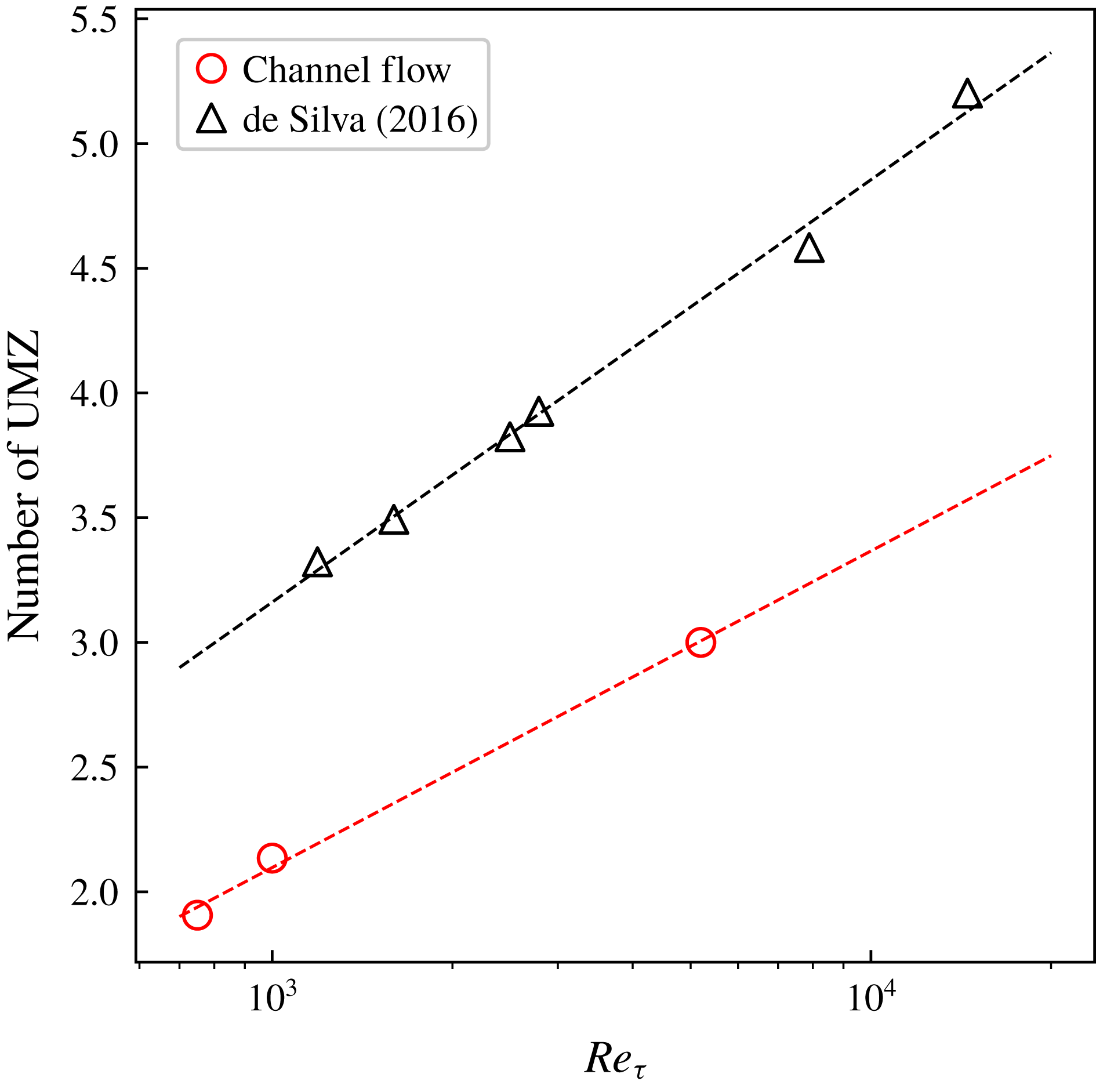
The number of UMZs has been shown to scale with the Reynolds number in boundary layer flows (de Silva et al. Reference de Silva, Hutchins and Marusic2016). Applying the KDE approach to an ensemble of two-dimensional slices to each of the turbulent channel flows in our database, we unambiguously and automatically identify the average number of UMZs as a function of the $Re_{\unicode[STIX]{x1D70F}}$ . For the analysis, we first randomly select individual slices in the three-dimensional snapshots, then we define a streamwise extent of $L_{x}=2000$ wall units and, finally, we run the KDE algorithm; the total number of peaks is recorded and averaged among all the slices for a given Reynolds number. As the KDE approach is based on an adaptive binning procedure, there was no user input required, thus making the approach robust and repeatable for all datasets. Figure 3 compares the computed number of UMZs from the channel flow database with the previously reported turbulent boundary layer (de Silva et al. Reference de Silva, Hutchins and Marusic2016). The variation of the number of zones with Reynolds number in the channel flow follows the same trend and slope as in the boundary layer, with the notable exception that the channel flow has fewer zonal hierarchies due to the constrained nature of the set-up. The limited $Re_{\unicode[STIX]{x1D70F}}$ -range of our datasets, especially between 1000 and 5000 but also above 5200, limits our ability to make any further claims on the observed difference in the channel and boundary layer flows.

Figure 3.

Average number of UMZs in turbulent channel flow databases computed based on the KDE algorithm. The comparative number of zones for the turbulent boundary layer, computed by de Silva et al. (Reference de Silva, Hutchins and Marusic2016), is shown in black.

Figure 4.

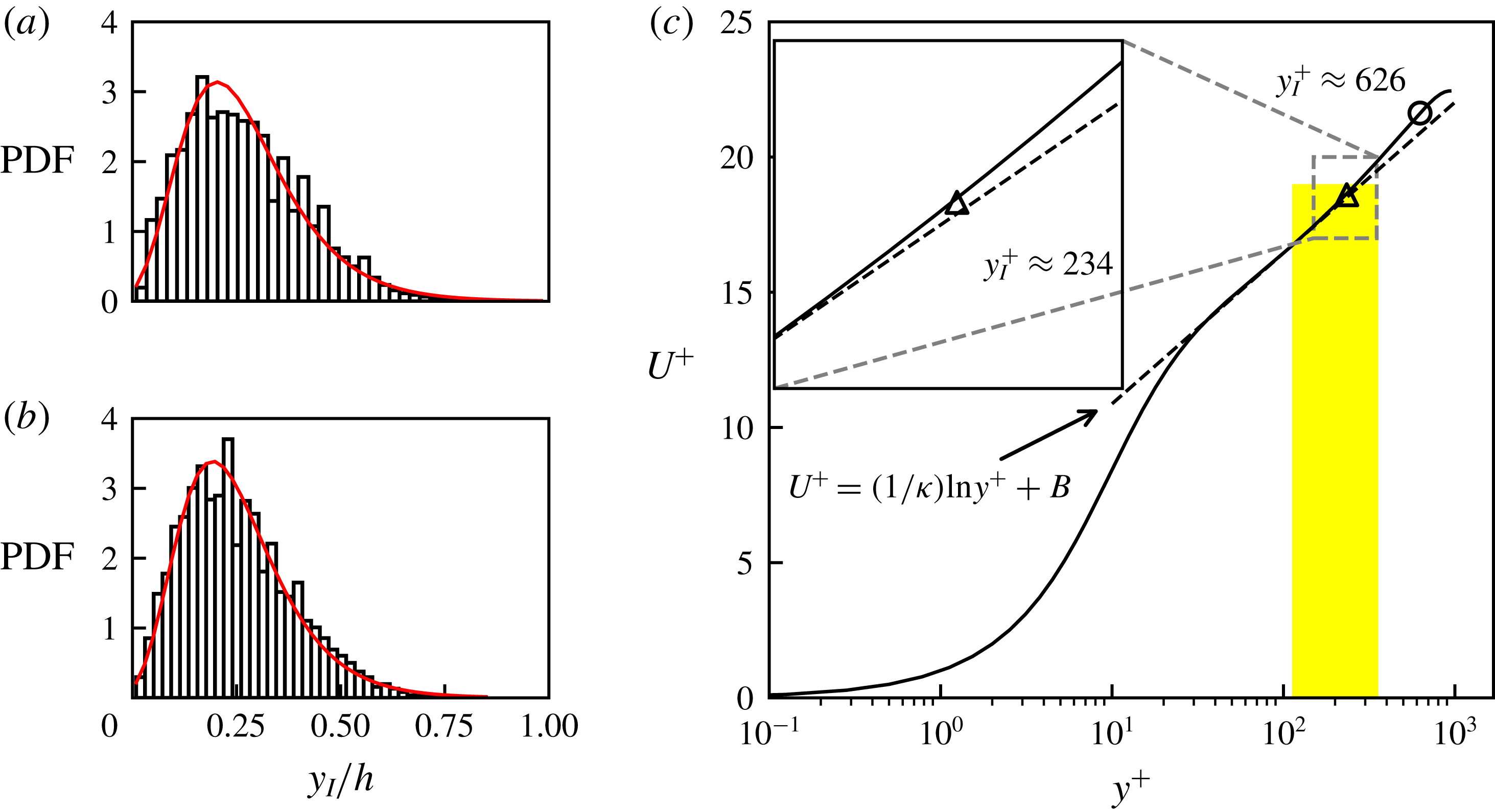
The distribution of the height of the IIL (between zones 2 and 3) for a turbulent channel flow at $Re_{\unicode[STIX]{x1D70F}}=550$ (a) and $950$ (b). The solid red lines correspond to a fitted log-normal probability distribution function. (c) Mean streamwise velocity profile (normalized in wall units) is shown relative to the mean height of IIL between zone 2 and 3 for $Re_{\unicode[STIX]{x1D70F}}=950$ . The log law $U^{+}=(1/\unicode[STIX]{x1D705})\ln (y^{+})+B$ (dashed line) is obtained by a linear fit of data between $y^{+}=3Re_{\unicode[STIX]{x1D70F}}^{1/2}$ and $0.15Re_{\unicode[STIX]{x1D70F}}$ ( $\unicode[STIX]{x1D705}=0.41$ ) following Marusic et al. (Reference Marusic, Monty, Hultmark and Smits2013). The mean height is highlighted by ▵ and ○ corresponds to the height of the quiescent core interface of Kwon et al. (Reference Kwon, Philip, de Silva, Hutchins and Monty2014). The width of the vertical bar denotes the standard deviation of the interface height.

Figure 5.

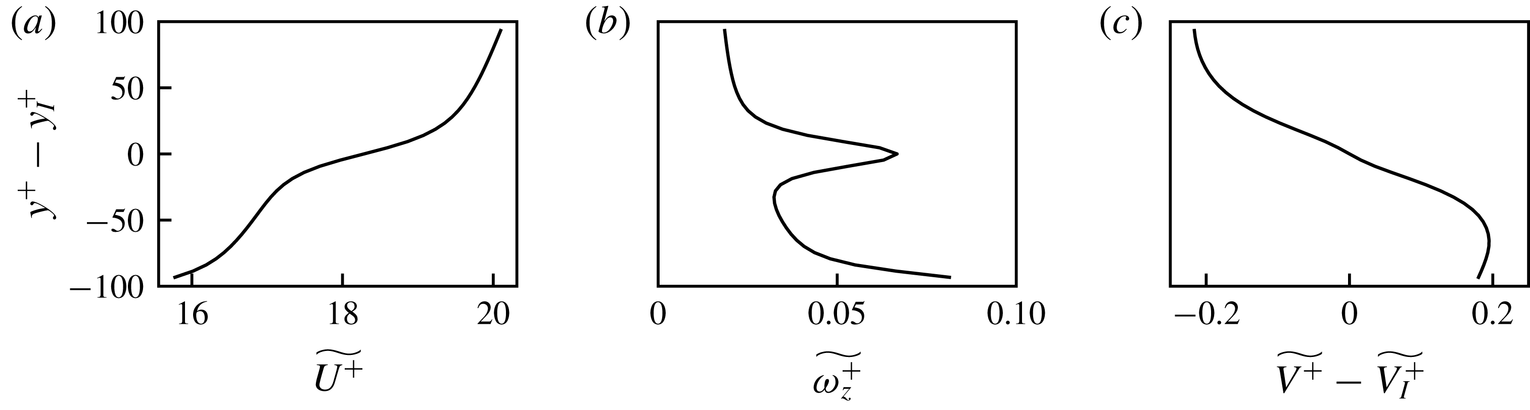
Conditional average across the IIL between zones 2 and 3 of the (a) streamwise velocity, (b) spanwise vorticity and (c) relative wall-normal velocity in the channel flow at $Re_{\unicode[STIX]{x1D70F}}=950$ .

Figure 6.

(a) Fluctuations of the IIL (between zones 2 and 3) normalized height for the channel flow at $Re_{\unicode[STIX]{x1D70F}}=950$ (Del Álamo et al. Reference Del Álamo, Jiménez, Zandonade and Moser2004). The raw data are low-pass filtered and re-sampled onto a coarser grid ( $\unicode[STIX]{x0394}x\times \unicode[STIX]{x0394}z=0.1h\times 0.1h$ ). (b) Streamwise (solid) and spanwise (dashed) autocorrelations of the IIL height fluctuation (computed using the raw data).

3.3.3 Interfacial layers and large-scale motion

The connection between interfacial layers and the large-scale motion (LSM) is investigated through the three-dimensional interfacial identification in the flow. The LSM is known to play an integral role in wall-bounded turbulent flows, and given its dynamic importance in the outer region, it has been shown that the LSM acts to modulate the TNTI in turbulent boundary layer flows (Lee, Sung & Zaki Reference Lee, Sung and Zaki2017). Many researchers, most notably Adrian et al. (Reference Adrian, Meinhart and Tomkins2000), have proposed conceptual frameworks to relate the UMZs, and ultimately LSM, to an alignment of hairpins vortices forming a hairpin packet; many of the foundational concepts of UMZs rest on Townsend’s understanding of a hierarchy of attached eddies (de Silva et al. Reference de Silva, Hutchins and Marusic2016). Underpinning many of these conceptual models is the idea that near-wall perturbations can be responsible for the dynamics within the outer region of wall-bounded flows.

Figure 7.

The cores of turbulent structures with a positive ( $+$ ) and negative (○) streamwise velocity fluctuations identified following the approach by Lee et al. (Reference Lee, Lee, Choi and Sung2014) on the turbulent channel flow at $Re_{\unicode[STIX]{x1D70F}}=1000$ (Lee & Moser Reference Lee and Moser2015). (a) Identified structure cores overlaid on the three-dimensional outer IIL; the IIL is coloured by the height relative to the wall. (b) Spanwise slice of the outer IIL taken at $x=8.0$ (identified in a); regions of positive and negative streamwise velocity fluctuations are shown for clarity.

The LSM, being primarily located in the outer region of the boundary layer, should also play a role in the modulation of the interfacial layers between the outer UMZs. Qualitatively, the LSMs are easily identified through any classical near-wall turbulent visualization approaches. Here, we rely on the formal streak detection algorithm proposed by Lee et al. (Reference Lee, Lee, Choi and Sung2014) to quantitatively identify the LSMs in order to relate them to the three-dimensional IILs. The streak detection rests on sequential data filtering of the streamwise velocity fluctuations (Gaussian followed by a long-wavelength-pass filter) and structure detection algorithms which are detailed in the referenced paper (Lee et al. Reference Lee, Lee, Choi and Sung2014). We investigate the channel flow at $Re_{\unicode[STIX]{x1D70F}}=1000$ (Lee & Moser Reference Lee and Moser2015) by extracting the characteristic splines (CS) which are located within a characteristic plane (CP); these splines are related to underlying characteristic structures, such as hairpin vortices (Lee et al. Reference Lee, Lee, Choi and Sung2014). Figure 7(a) shows the location of the positive ( $+$ ) and negative (○) characteristic splines in three dimensions; the outer interfacial layer (between zones 2 and 3) – identified through our clustering algorithm – is shown coloured by its height from the wall. Here, we clearly identify the very long positive and negative streamwise velocity regions in the flow. The three-dimensional visualizations show that in the valleys of the IIL, an alignment of coherent structures with a positive streamwise velocity fluctuation is found. Conversely, structures with a negative streamwise fluctuation concentrate along the ridges of the IIL. This observation correlates with the ejection and sweep-type mechanisms that are typical for these types of near-wall structures. The ability to define three-dimensional interfaces supports the postulated relationship between the near-wall structures and the interfacial layers in wall-bounded turbulence (de Silva et al. Reference de Silva, Philip, Hutchins and Marusic2017).

The connection between the outer IIL and LSM is clearly seen in the $y/z$ slice at a constant streamwise location in figure 7(b). By overlaying locally filtered regions of positive and negative streamwise velocity, we show that the IIL is modulated by the LSM in the outer layer of the boundary. Based on these qualitative observations, it is also expected that these same LSMs modulate the near-wall IIL. To this end, we compute the cross-correlation coefficient of the IIL height of the inner and outer IIL. A slightly positive correlation coefficient (0.103) is observed between the height of both layers, which can be explained by the skewness resulting from the presence of the wall. A small correlation is not too surprising as the interfacial heights at these two very distant locations in the boundary layer should be, for the most part, dynamically independent. By conditionally sampling the data to only consider the locations of peak near-wall events – where the height of the inner IIL is greater than one standard deviation from the mean – a significantly higher correlation is noted (0.22). In other words, near-wall events that significantly modify the local interfacial height can be felt in the outer part of the near-wall boundary layer in these flows.

4.1 Sensitivity to the number of IILs

The FCM requires a user-defined number of internal zones, $K$ , as an a priori input for clustering. In § 2, we proposed a method to automatically determine the number of internal zones in a given flow snapshot based on a kernel density estimation (KDE). The question then arises: how sensitive is the FCM identification if the wrong number of internal zones, $K$ , is provided as input? It is understood that if the incorrect number of zones is selected as an input to the algorithm for a given snapshot, the physical interpretation of the UMZs would be incorrect. Nonetheless, we show that the identification of the most important internal layers is insensitive to the number of zones if the error in $K$ is $\pm 1$ . Figure 8 shows the IILs of a single slice of the high-Reynolds-number channel flow DNS by Lee & Moser (Reference Lee and Moser2015) using three ( $K=3$ , full line) and four ( $K=4$ , dashed line) internal zones (with respectively two and three IILs). The same two IILs are identified using a different number of clusters: very near the wall and at the outer edge of the boundary layer. When clustering on four zones (three IILs) instead of three (two IILs), an additional interface is identified. In other words, the approach remains robust to a small error in the a priori quantification of the number of zones. This same analysis was also conducted using five zones with similar results. It should be noted that on lower-Reynolds-number datasets, the result showed a slightly greater sensitivity to the error. Although this sensitivity analysis highlights the robustness of the algorithm to the selection of the number of zones, the physical interpretation of the results would differ greatly if an incorrect number of zones were used. Therefore, it is essential to carefully conduct an a priori KDE analysis to assess the correct number of zones for a given snapshot in a dataset.

Figure 8.

The IIL overlaid on the streamwise velocity contour plot for a high-Reynolds-number channel flow (Lee & Moser Reference Lee and Moser2015). The black solid lines are the identified IILs initialized with three internal zones and the red dotted lines are the identified IILs initialized with four internal zones.

4.2 Sensitivity to initialization

One of the shortcomings of many data clustering approaches lies in the sensitivity of the final cluster to the initialization. In order to initiate the fuzzy cluster algorithm, the membership functions, $u_{mk}$ , must be initialized. The number of membership functions is the same as the a priori determined number of clusters, $K$ . Suppose we have three clusters ( $K=3$ ), the sum of all of the membership functions at each $m$ grid points is

(4.1) $$\begin{eqnarray}\displaystyle u_{m1}+u_{m2}+u_{m3}=1. & & \displaystyle\end{eqnarray}$$

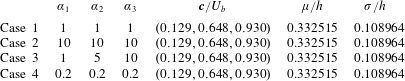
To study the sensitivity of the FCM, we randomly select the initial membership function centroids in order to test the robustness of the method to the initialization. A three-dimensional Dirichlet probability distribution is used to randomly select the centroids for initialization. 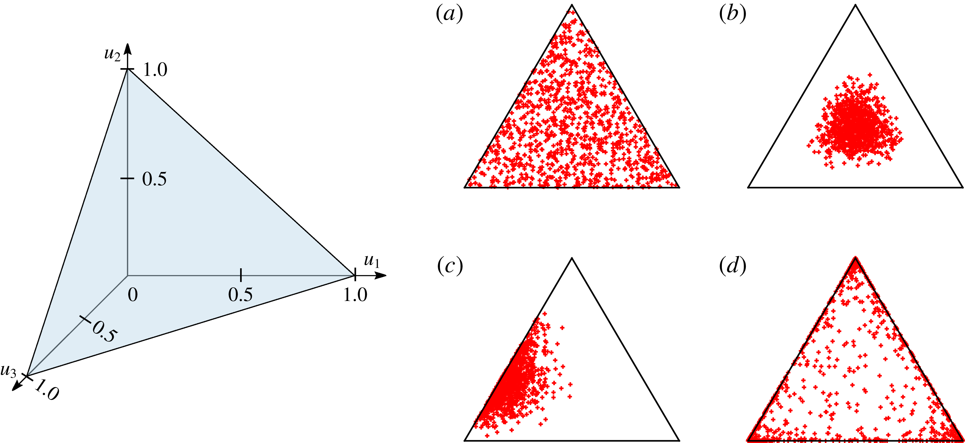The Dirichlet distribution is fully defined by three independent parameters ( $\unicode[STIX]{x1D6FC}_{1},\unicode[STIX]{x1D6FC}_{2},\unicode[STIX]{x1D6FC}_{3}$ ), and under the proper normalization, the sum of the membership functions is unity. Figure 9 shows the tested Dirichlet probability distributions for initialization; each point in the triangle must have a value constrained between 0 and 1 in each dimension and must sum up to one. Irrespective of our selected initialization, exactly the same IILs (height, statistics and centroids) are identified for the channel flow simulation at $Re_{\unicode[STIX]{x1D70F}}=950$ (centreplane slice). The statistics on the modal velocities, the normalized height of the interface ( $\unicode[STIX]{x1D707}/h$ ) and its standard deviation $\unicode[STIX]{x1D70E}/h$ are shown in table 2. These results clearly show that the method remains robust to the initialization of the problem.

Figure 9.

The Dirichlet distribution of the membership function initialization where each side of the triangle represents the initialization of one of the membership functions. The points in the triangle must simultaneously satisfy two constraints: the value must be constrained between 0 and 1 in each dimension and must sum up to 1 (see illustration on left side). The parameters used to defined the Dirichlet probability distribution are $\unicode[STIX]{x1D6FC}_{1},\unicode[STIX]{x1D6FC}_{2},\unicode[STIX]{x1D6FC}_{3}$ . The above distributions represent (see table 2): (a) Case 1; (b) Case 2; (c) Case 3; and (d) Case 4.

Table 2.

Dirichlet distribution parameters, converged cluster centroid and statistics ( $\unicode[STIX]{x1D707}$  and $\unicode[STIX]{x1D70E}$ are respectively the mean and standard deviation of the interfacial height) of the IIL between zones 2 and 3 for Cases 1, 2, 3 and 4.

4.3 IIL identification under stochastic perturbations

As the clustering approach remains agnostic of the underlying physics of the flow, we test the robustness of the interfacial identification to initial perturbations to the data. Such perturbations could arise from experimental noise or discretization errors. Using the same initial membership functions (with a defined number of clusters), we perturb the raw data with white noise; here we use the channel flow at $Re_{\unicode[STIX]{x1D70F}}=1000$ for reporting the analysis; similar findings are observed on the other data. We perturb the numerical data with up to 50 % white noise based on the bulk velocity of the flow. To show the robustness of the method, the perturbations are not damped down to the wall, thus creating a non-physical noise. Figure 10(a) shows the effect of the white noise on the identification of the cluster centres (which correspond to the modal velocities of internal zones); under 15 % noise, very little variation in the modal velocity is noted. The effect of the added noise on the average height of the IIL is presented in figure 10(b). The average height of the interface and its standard deviation remains constant up to 15 % white noise. Figure 10(c) shows the outer envelope of the ILL, between zones 2 and 3, under 0 % (left), 5 % (centre), and 10 % (right) random perturbations. We note that similar interface geometries can be captured despite the added noise.

Figure 10.

Robustness of the FCM against initial perturbations to the data. (a) Shows the effect of white noise on the identified cluster centres centroids; each line corresponds to the modal velocity of the UMZs. As the amplitude of the noise increases (above, say, 15 %), the ability to capture the cluster centre decreases. (b) Shows the average height of the IIL between zones 2 and 3 (solid line) and the standard deviation (dashed line) as a function of the imposed noise to the data. (c) Shows the IIL between zones 2 and 3 under 0 % (solid), 5 % (dash-dotted), 10 % (dotted), and 30 % (dashed) white noise. (c) Shows the IIL between zones 2 and 3 under 0 %, 5 % and 10 % noise (from left to right) at the same streamwise plane view. Grid points are coloured based on the zones and the solid black line represents the outer envelope of the IIL.