Nomenclature
- Symbol
-
Definition
-
 $(c), (C)$
-
Local blade chord length
-
$(C_D)$
-
Drag coefficient
-
$(C_L)$
-
Lift coefficient
-
$(C_P)$
-
Power coefficient
-
$(C_T)$
-
Thrust coefficient
-
$(dQ)$
-
Differential aerodynamic torque
-
$(dT)$
-
Differential thrust
-
$(F)$
-
Prandtl tip-loss correction factor
-
$(J)$
-
Advance ratio
-
$(M)$
-
Mach number
-
$(N)$
-
Number of blades or samples, as defined in context
-
$(P_L)$
-
Motor power loss
-
$(P_{\mathrm{shaft}})$
-
Propeller shaft power
-
$(Q)$
-
Propeller aerodynamic torque
-
$(r)$
-
Radial position
-
$(R)$
-
Propeller radius
-
$(Re)$
-
Reynolds number
-
$(T)$
-
Total propeller thrust
-
$(V)$
-
Flight or inflow velocity
-
$(V_{ia})$
-
Axial induced velocity
-
$(V_R)$
-
Local relative velocity
-
$(W), (b)$
-
Neural-network weights and biases
-
$(\mathbf{x})$
-
Input or design-variable vector
-
$(\mathbf{y})$
-
Aerodynamic output vector


1.0 Introduction
High-altitude long-endurance (HALE) solar-powered unmanned aerial vehicles (UAVs), or ‘pseudo-satellites’, operate above 20 km in the stratosphere, where low air density results in propellers functioning at very low Reynolds numbers (104–105). This induces laminar separation bubbles and transition phenomena, sharply reducing aerodynamic efficiency and posing challenges for propeller design. Solar UAV propulsion systems consist of motors and propellers, which must achieve lightweight structure, high efficiency and effective propeller–motor matching. Performance depends on coordinated matching of power, rotational speed, chord and pitch angle at the design flight condition [Reference Shengqi1–Reference Leishman and Rosen3]
Propellers are affected by blade-vortex interactions and tip compressibility effects, which increase power loss. Rotor aerodynamic shape prediction methods mainly include the traditional iterative solution approach based on blade element momentum theory (BEMT) and high-fidelity computational fluid dynamics (CFD). In particular, BEMT solves the coupled momentum and blade-element equations through iterative convergence of induced velocity and sectional forces, providing an efficient semi-empirical framework for rotor performance prediction [Reference Gur and Rosen4, Reference Stahlhut5]. With Prandtl tip-loss correction, BEMT offers a balance between computational efficiency and acceptable accuracy. Prior studies investigated rotor-wing interactions, multi-objective optimisation and propeller design using genetic or particle swarm algorithms, with validation by wind tunnel experiments [Reference Lei and Xile6–Reference Tran and Lim12].
High-fidelity CFD is computationally expensive for iterative optimisation. Surrogate models, including the Reynolds stress model (RSM), Kriging, multilayer perceptrons (MLPs) and convolutional neural networks (CNNs), have been applied to accelerate predictions but are limited in capturing highly nonlinear aerodynamic behaviour at low Reynolds numbers [Reference Cai13–Reference Zhang, Sung and Mavris21].
However, deep learning methods integrating a residual network (ResNet) with Bayesian optimisation for full-envelope aerodynamic shape prediction of low-Reynolds-number UAV propellers remain limited. A key challenge in deep neural networks is the degradation problem, where increasing network depth leads to higher training error rather than performance improvement due to optimisation difficulty and gradient degradation. Residual learning with skip connections effectively mitigates this issue by enabling identity mapping and improving gradient propagation in deep architectures [Reference He22]. This makes ResNet particularly suitable for modeling strongly nonlinear aerodynamic responses under low-Reynolds-number conditions.
The use of a residual fully connected network is consistent with the nature of the present regression problem. The input variables, including Reynolds number, Mach number and angle-of-attack, form a low-dimensional continuous parameter vector, without image-like spatial features or temporal sequence dependencies. Therefore, CNN- or recurrent neural network (RNN)-based architectures are not the most natural choices for this task. In contrast, a fully connected residual network is well suited for learning nonlinear mappings from aerodynamic states to lift and drag coefficients. Its skip connections help alleviate degradation as network depth increases by enabling residual correction learning and stable gradient propagation. Bayesian optimisation is further used to select key hyperparameters, such as network depth, hidden-layer width, learning rate, weight decay and batch size, thereby reducing empirical trial-and-error. Accordingly, the proposed Bayesian optimised aerodynamic residual network (BO-ARN) model functions as a task-specific and computationally efficient surrogate for XFoil-supported BEMT analysis under low-Reynolds-number HALE UAV propeller conditions. This study proposes an integrated framework combining BEMT, a BO-ARN and a genetic algorithm (GA) for rapid performance prediction and global optimisation of propeller chord and twist. The BO-ARN surrogate replaces repeated XFoil evaluations, predicting lift, drag, thrust, torque and induced velocity, while the GA optimises propeller geometry under motor power and torque constraints [Reference Khan and Nahon23].
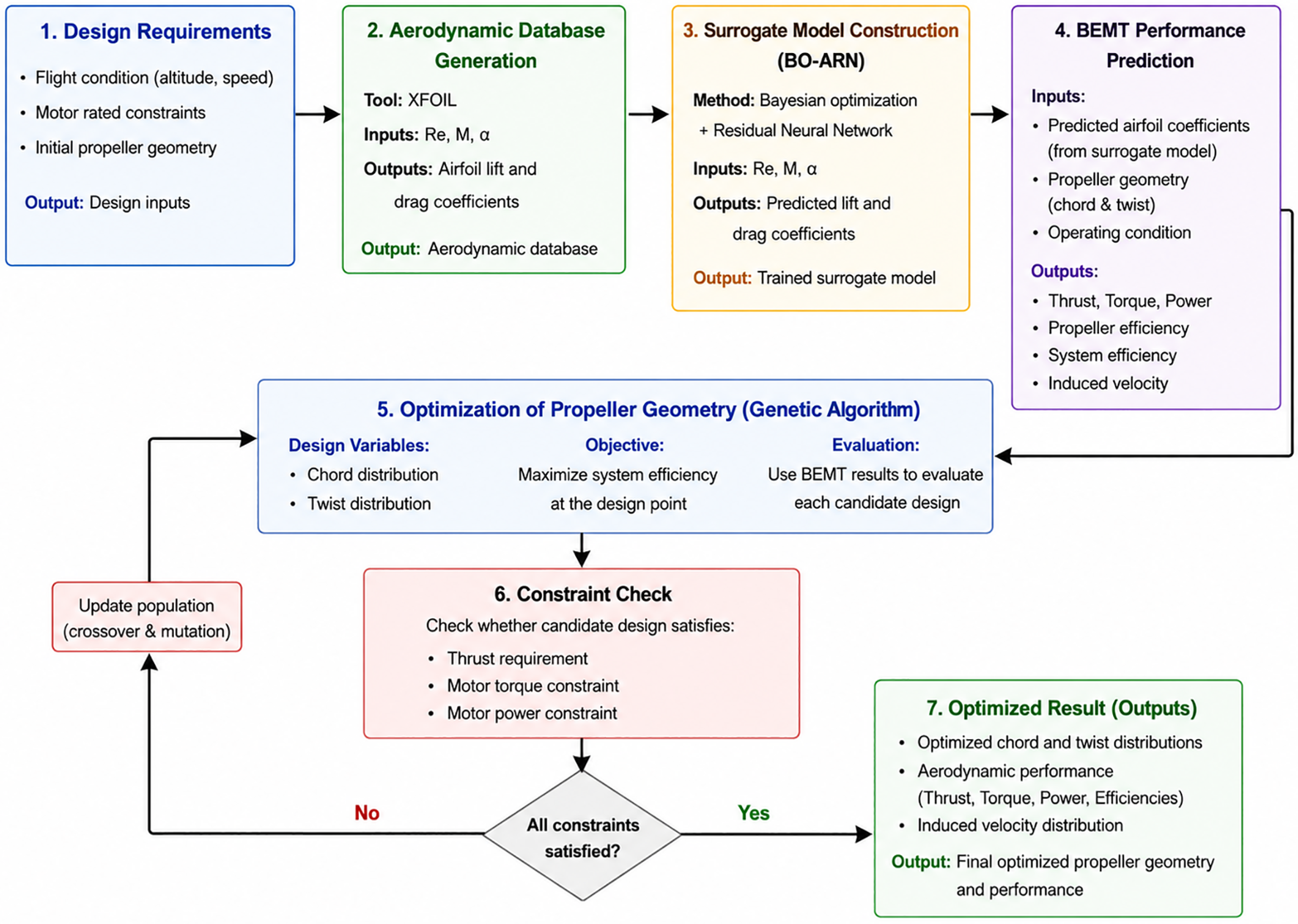
The novelty of this work is threefold: (1) development of an RNN optimised via Bayesian hyperparameter search to accurately predict low-Re aerodynamic coefficients, overcoming the degradation problem in deep networks; (2) embedding BO-ARN into BEMT to establish rapid propeller performance prediction; (3) proposing a system-level optimisation strategy to maximise cruise efficiency while explicitly considering propeller–motor matching. As illustrated in Fig. 1, this framework provides an efficient and practical tool for designing high-altitude solar UAV propulsion systems.
Overall workflow of the proposed BEMT–BO-ARN–GA propeller optimisation framework.

Figure 1. Long description
The flowchart illustrates the optimization framework for propeller design in high-altitude long-endurance solar-powered unmanned aerial vehicles. Panel 1: Design Requirements. Flight condition, motor rated constraints, and initial propeller geometry are the inputs. Output: Design inputs. Panel 2: Aerodynamic Database Generation. Tool: XFOIL. Inputs: Re, M, alpha. Outputs: Airfoil lift and drag coefficients. Output: Aerodynamic database. Panel 3: Surrogate Model Construction (BO-ARN). Method: Bayesian optimization + Residual Neural Network. Inputs: Re, M, alpha. Outputs: Predicted lift and drag coefficients. Output: Trained surrogate model. Panel 4: BEMT Performance Prediction. Inputs: Predicted airfoil coefficients, propeller geometry, and operating condition. Outputs: Thrust, Torque, Power, Propeller efficiency, System efficiency, and Induced velocity. Panel 5: Optimization of Propeller Geometry (Genetic Algorithm). Design Variables: Chord distribution, Twist distribution. Objective: Maximize system efficiency at the design point. Evaluation: Use BEMT results to evaluate each candidate design. Panel 6: Constraint Check. Check whether candidate design satisfies thrust requirement, motor torque constraint, and motor power constraint. If all constraints are satisfied, proceed to Panel 7. If no, update population (crossover & mutation) and return to Panel 5. Panel 7: Optimized Result (Outputs). Outputs: Optimized chord and twist distributions, Aerodynamic performance, Induced velocity distribution. Output: Final optimized propeller geometry and performance.
2.0 Blade element momentum theory model
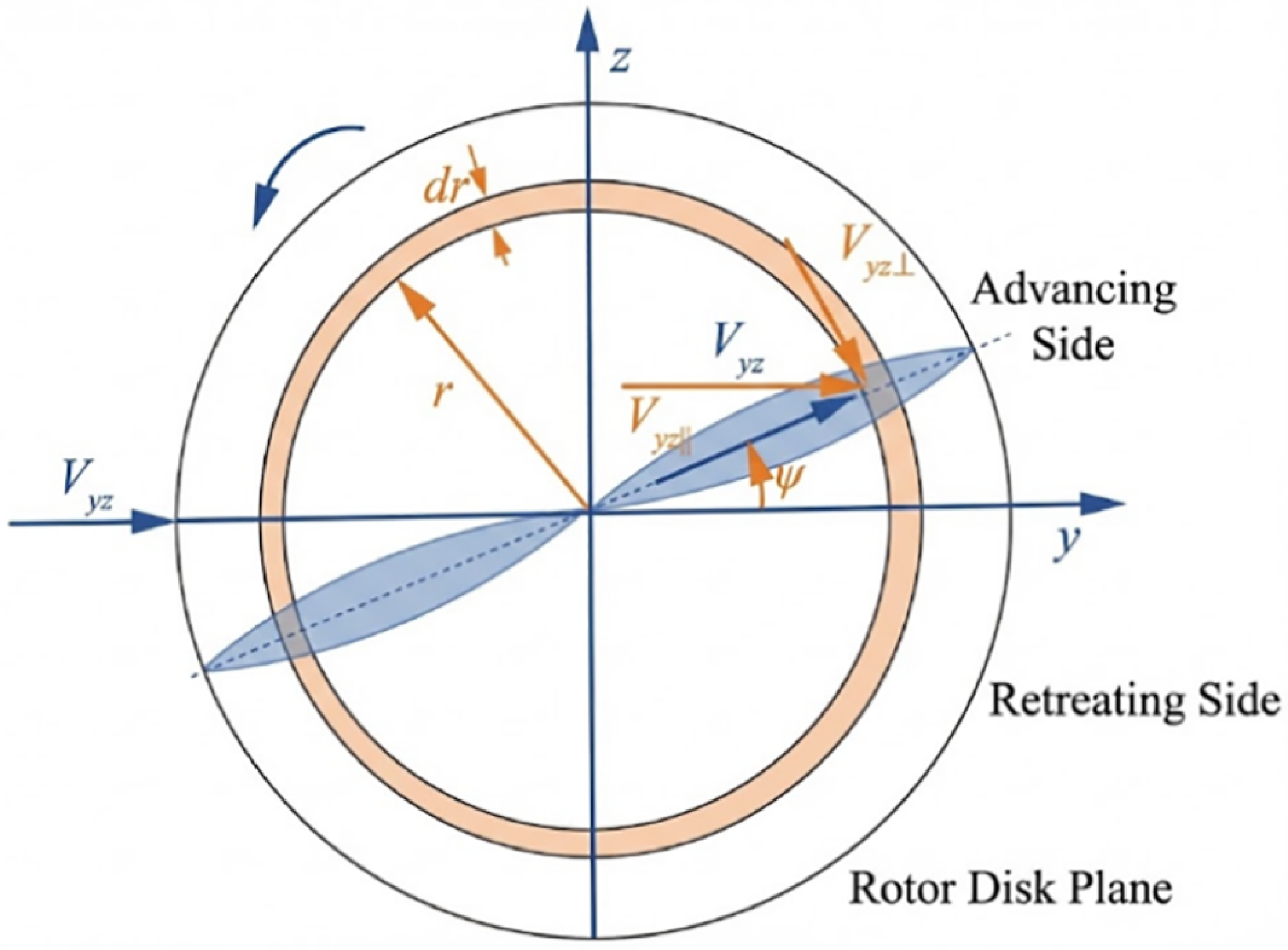
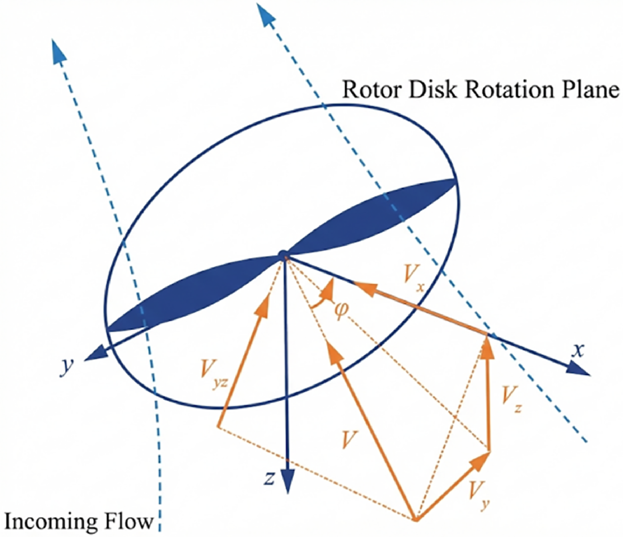
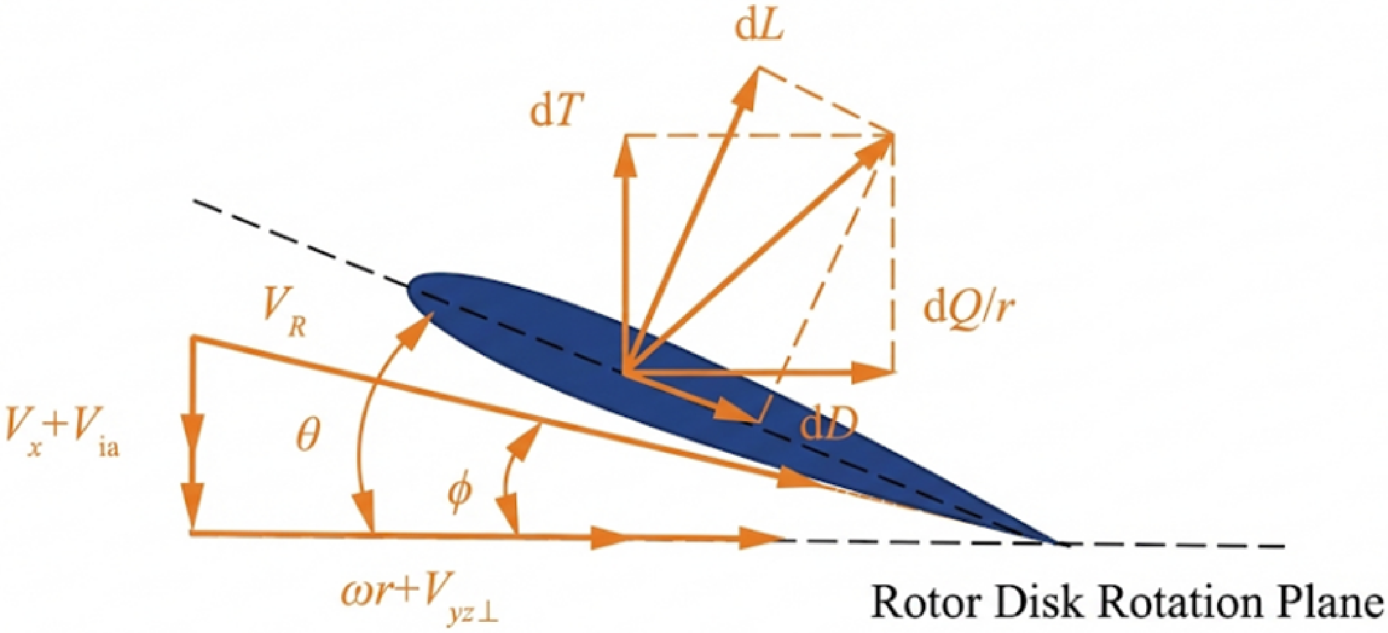
BEMT, with its excellent balance between computational accuracy and efficiency, has become the preferred method for rotor aerodynamic shape optimisation, offering significant advantages over high-computational-cost CFD simulations. BEMT combines the macroscopic control volume analysis of momentum theory with the microscopic profile analysis of blade element theory (BET): the former is based on the uniform slipstream hypothesis, equating the rotor to a zero-thickness actuator disk that generates a pressure difference. The latter discretises the blade into infinite infinitesimal segments, determining the forces by analysing local geometric parameters and kinematic characteristics. By coupling these two theories and iteratively solving for the induced velocity distributed along the radial direction, the calculation of the overall aerodynamic forces and power characteristics of the rotor can be achieved. As shown in Figs 2 and 3, due to issues such as tip losses during the high-speed rotation of the rotor, the momentum theory formula incorporating Prandtl’s approximation function for tip loss correction is as follows [Reference Wang24]:
 \begin{equation}\begin{array}{l}dT = 2\rho r\int_{\psi = 0}^{2\pi } {{V_u}} \sqrt {{{({V_x} + {V_{ia}})}^2} + V_{y \bot }^2} \mathbb{F}d\psi dr\\dQ = 2\rho {r^2}\int_{\psi = 0}^{2\pi } {(\omega r + {V_{y \bot }})} \sqrt {{{({V_x} + {V_{ia}})}^2} + V_u^2} \mathbb{F}d\psi dr\end{array}\end{equation}
where dT represents the thrust of the blade element segment, dQ represents the torque of the blade element segment around the rotation axis and Vx represents the axial component of the inflow velocity along the rotation axis:
 \begin{equation}{V_x} = V\cos \varphi \end{equation}
where
 $\varphi $
represents the angle between the inflow velocity and the rotation axis;
 ${V_{y \bot }}$
represents the component of the inflow velocity on the rotation plane perpendicular to the blade:
 \begin{equation}{V_{yz \bot }} = {V_{yz}}\sin \psi \end{equation}
Schematic diagram of oblique influx [Reference Wang24].

Rotating plane top view [Reference Wang24].

 $\psi $
is the blade rotation azimuthal angle, with the plane inflow direction defined as the y-axis and the direction parallel to the y-axis as the 0° azimuth. V
ia,0
represents the induced velocity at the centre of the rotor disk rotation, and the axial induced velocity V
ia
can be expressed as:
 \begin{equation}{V_{ia}} = {V_{ia,0}}\left( {1 + \frac{{15\pi }}{{32}}\tan \left( {\frac{\chi }{2}} \right)\frac{r}{R}\cos \psi } \right)\end{equation}
where the wake skew angle
 $\chi $
can be expressed as:
 \begin{equation}\chi = \arctan \left( {\frac{{{V_{yz}}}}{{{V_x} + {V_{ia,0}}}}} \right)\end{equation}
 $\mathbb{F}$
is the Prandtl tip loss correction function:
 \begin{equation}\mathbb{F} = \frac{2}{\pi }\arccos \left( {\exp \left( {\frac{{ - (R - r)N}}{{2r\sin \phi }}} \right)} \right)\end{equation}
where N represents the number of rotor blades, R represents the rotation radius, r represents the radial position and the inflow angle
 $\phi $
can be expressed as:
 \begin{equation}\phi = \arctan \left( {\frac{{{V_x} + {V_{ia}}}}{{\omega r + {V_{yz \bot }}}}} \right)\end{equation}
As shown in Fig. 4, the formulas for BET are:
 \begin{equation}\begin{array}{rl}dT &= \dfrac{N}{{4\pi }}\rho c\int_{\psi = 0}^{2\pi } {V_R^2} ({C_l}\cos \phi - {C_d}\sin \phi )d\psi dr\\[10pt] dQ &= \dfrac{N}{{4\pi }}\rho cr\int_{\psi = 0}^{2\pi } {V_R^2} ({C_l}\sin \phi + {C_d}\cos \phi )d\psi dr\\[10pt]V_R &= \sqrt {{{({V_x} + {V_{ia}})}^2} + {{(\omega r + {V_{y \bot }})}^2}} \end{array}\end{equation}
Blade element theory [Reference Wang24].

Figure 4. Long description
A diagram of the blade rotation azimuthal angle in a rotor disk rotation plane. The diagram shows a blade element with various forces and velocities acting on it. The plane inflow direction is defined as the y-axis, and the direction parallel to the y-axis is the 0 azimuth. The induced velocity at the center of the rotor disk rotation is represented as Via,0. The axial induced velocity Via can be expressed as a function of the wake skew angle. The diagram includes labels for different forces and velocities, such as dL, dT, dQ/r, dD, VR, θ, φ, and ωr+Vyz⊥. Arrows indicate the direction of these forces and velocities, showing their relationships and interactions within the rotor disk rotation plane.
By simultaneously coupling Equations (1) and (8), the induced velocity is iteratively solved using the Brent method, which is then substituted back into the equations to obtain the thrust and torque.
3.0 Validation of the BEMT method
To establish the reliability of the aerodynamic analysis framework, a two-step validation strategy was adopted in this study. First, the BEMT method was compared with available wind-tunnel experimental data to demonstrate its feasibility in predicting the general aerodynamic performance trends of low-Reynolds-number propellers. Subsequently, CFD simulations were further conducted for the propeller model used in this study to verify the applicability of the BEMT method to the present blade geometry and high-altitude operating conditions. Through these two levels of validation, the BEMT-based calculation model was shown to provide sufficient accuracy and computational efficiency for subsequent surrogate-model construction and propeller optimisation.
3.1 Verification of BEMT and experiment aerodynamic performance
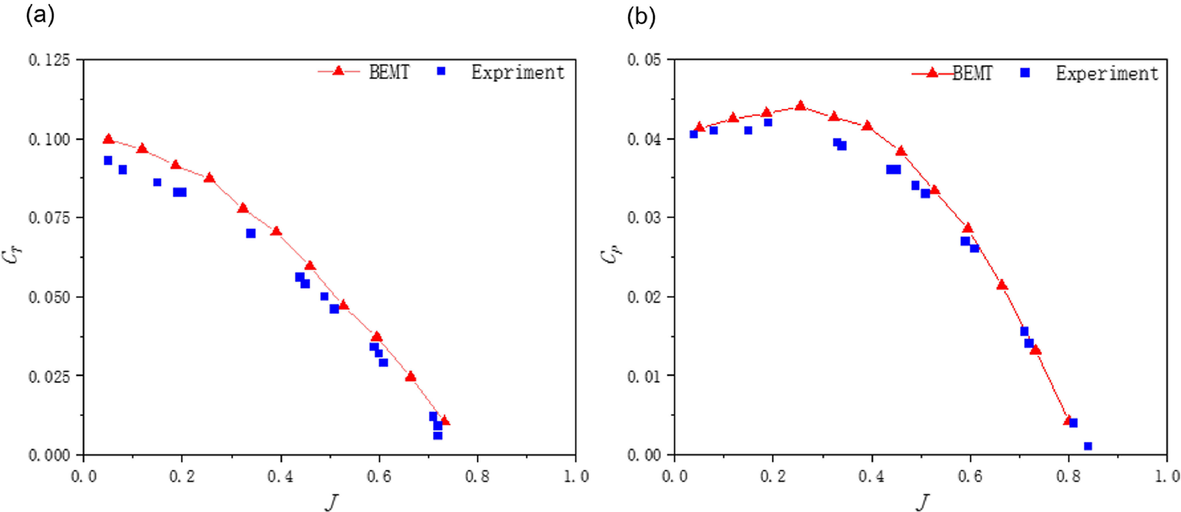
To verify the accuracy of the BEMT method under real wind-tunnel experimental conditions, a two-bladed propeller with a diameter of 6 inches was selected as the validation case [Reference Ghoddoussi and Miller25]. The propeller adopts the E387 aerofoil, with the last 10% of the trailing edge removed to satisfy manufacturing requirements, and its blade twist angle at the 75% radial station is 15°. The experiment was conducted at approximately 6,000 rpm, corresponding to an operating Reynolds number of Re9.0 × 104–1.2 × 10⁵ at the 75% radial section, which is representative of typical low-Reynolds-number propeller operating conditions. The variations of the thrust coefficient C T and power coefficient C P with the advance ratio (J), obtained using the BEMT-based rapid calculation method, are compared with the wind-tunnel measurements. As illustrated in Fig. 5, the results show that the BEMT predictions can reasonably capture the overall trends of the experimental curves. Specifically, as the advance ratio J increases, the thrust coefficient decreases continuously, while the power coefficient remains relatively stable at low advance ratios and then decreases markedly with further increase in J. Although certain discrepancies exist between the BEMT results and the experimental data, good agreement is observed within the main operating range, indicating that the BEMT-based method can reliably reflect the fundamental aerodynamic performance characteristics of low-Reynolds-number propellers.
Comparison between BEMT predictions and experimental results: (a) comparison of CT between BEMT predictions and experimental results and (b) comparison of CP between BEMT predictions and experimental results.

3.2 Verification of BEMT and CFD aerodynamic performance
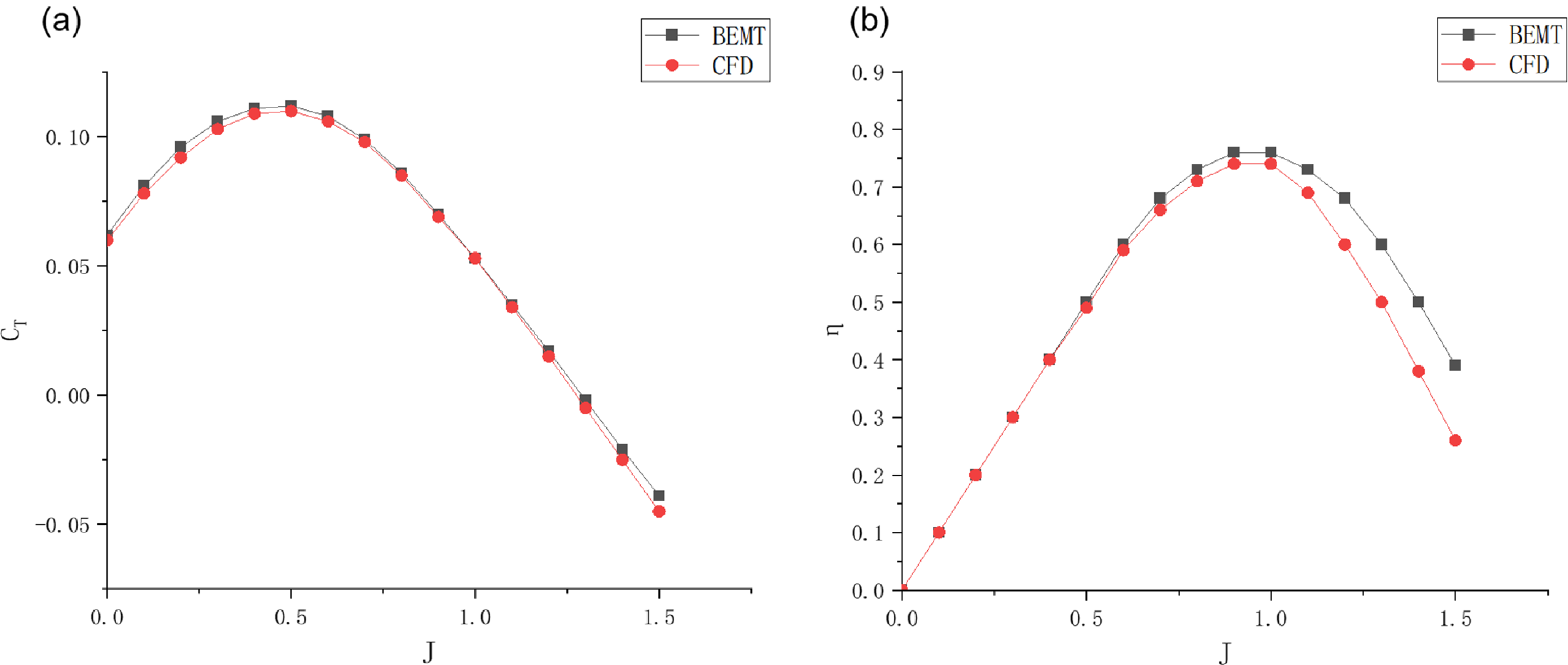
To verify the accuracy of the BEMT calculation model for predicting propeller performance in high-altitude environments (taking a two-bladed propeller operating at an altitude of 25 km, a forward speed of 40 m/s, and a rotational speed of 1,200 rpm as an example), the thrust coefficient C
T
and calculated efficiency
 $\eta$
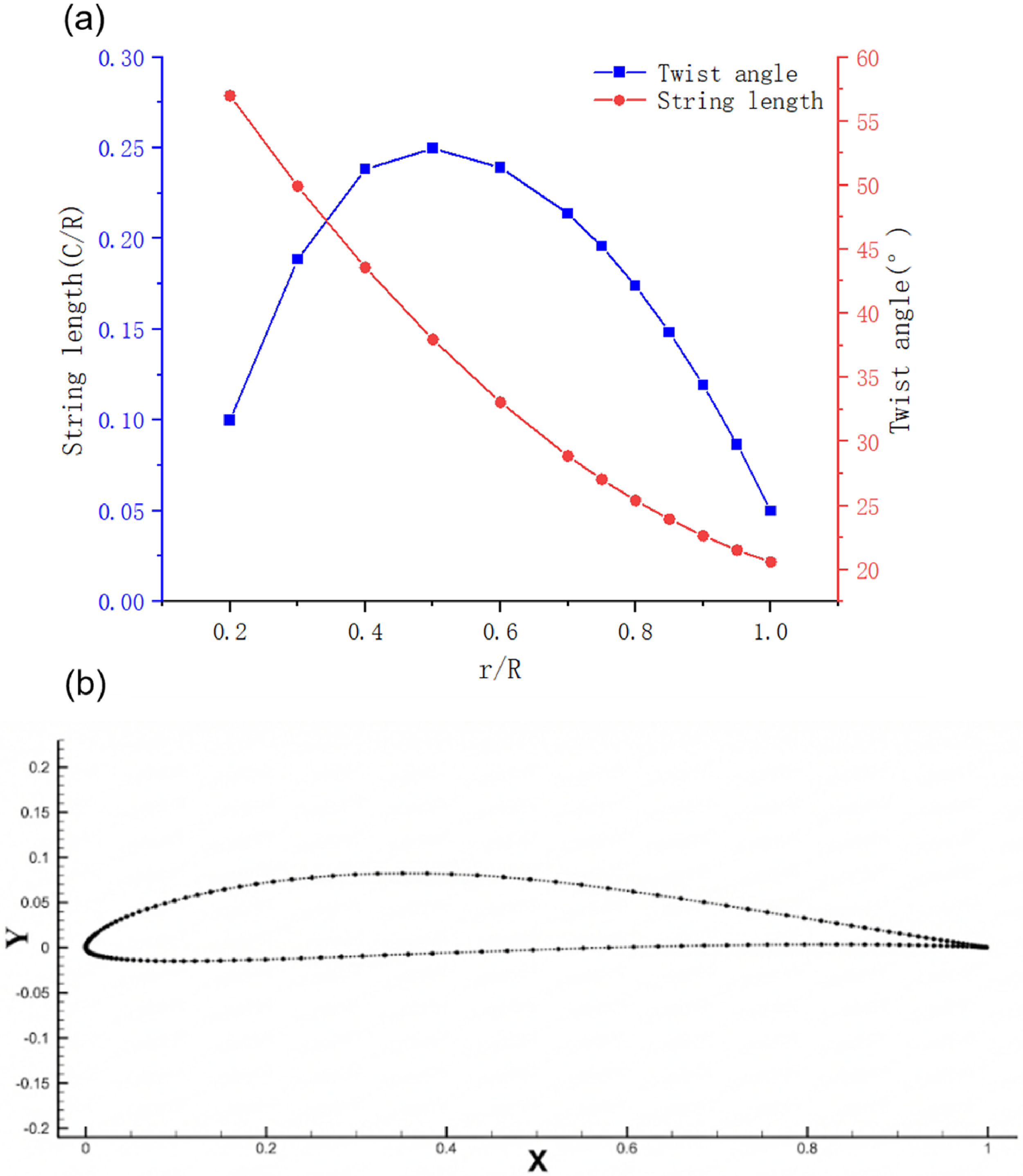
obtained by BEMT and CFD methods at different advance ratios J were analysed and compared to validate the precision of the BEMT model. This study utilises XFoil to calculate the lift and drag coefficients of each blade element, performing BEMT calculations based on the XFoil results. The E387 aerofoil was selected [Reference Ghoddoussi and Miller25], and the geometric design parameters and aerofoil of the propeller are shown in Fig. 6.
Propeller geometric model: (a) propeller geometric parameters and (b) schematic diagram of the propeller blade.

Figure 6. Long description
Panel A: A line graph shows the relationship between propeller geometric parameters. The x-axis is labeled r/R, the y-axis on the left is labeled String length (C/R), and the y-axis on the right is labeled Twist angle (degrees). The graph includes two data series: one for twist angle represented by blue squares and one for string length represented by red circles. The twist angle increases to a peak around r/R of 0.5 and then decreases, while the string length decreases steadily. Panel B: A scatter plot shows the schematic diagram of the propeller blade. The x-axis is labeled X and the y-axis is labeled Y. The data points form a curved shape representing the blade’s geometry.
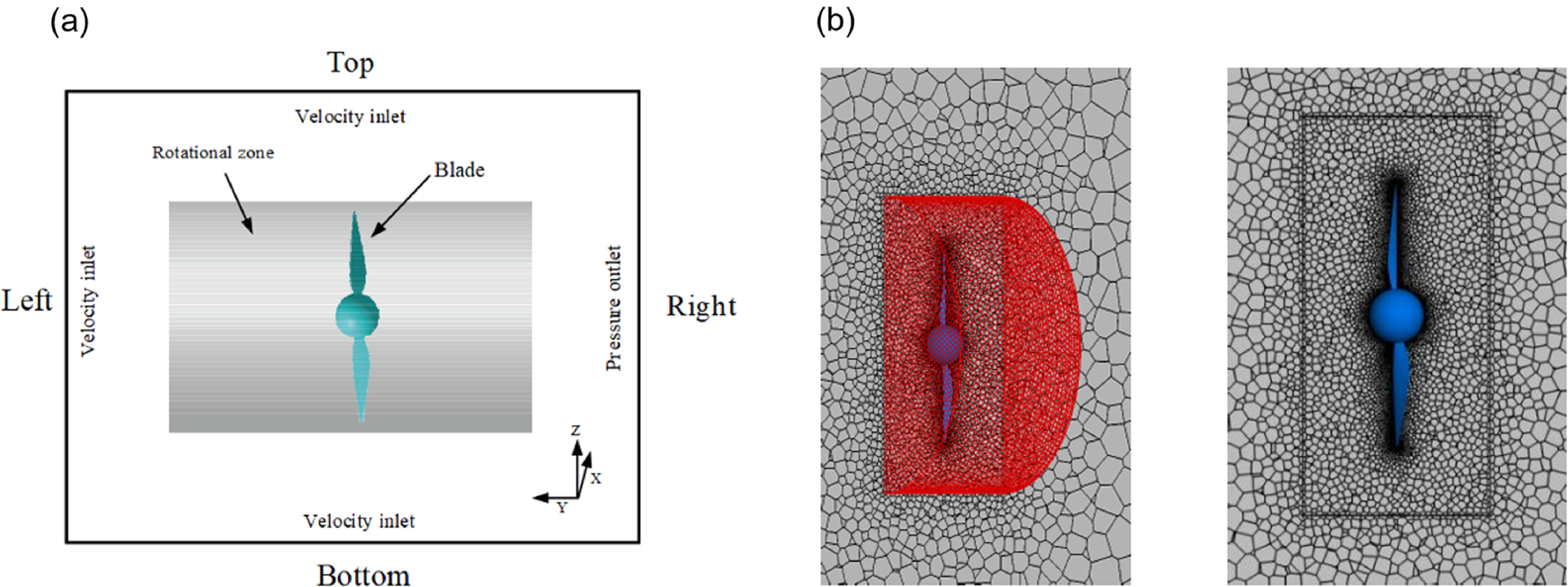
In the CFD simulation, the fluid domain is modeled as a rectangular parallelepiped, with the right surface as a pressure outlet and other surfaces as velocity inlets; a cylinder simulates the internal rotating domain, and the rotating region is connected to the fluid domain via an interface. A polyhedral mesh was selected for the discretisation of the fluid domain. During the flow field simulation, the RSM turbulence model was employed, as shown in the CFD simulation (Fig. 7).
Propeller CFD simulation setup: (a) schematic diagram of propeller flow field simulation and (b) propeller flow field mesh.

In the results shown in Fig. 8, the efficiency and thrust coefficient calculated by the two methods vary similarly with the advance ratio J, indicating that under high-altitude low-density conditions, the propeller performance predicted by the BEMT method is approximately the same as the results obtained through the CFD method. When the advance ratio
 $J \lt 1$
, the difference in thrust coefficient and efficiency between the BEMT and CFD methods is small, indicating that in low-speed flight or hover stages, both methods can reliably predict the propeller’s thrust output; when
 $J \gt 1$
, as the propeller speed increases, the surrounding flow field becomes more complex, involving strong three-dimensional and unsteady effects. CFD simulations are expected to be more accurate as they consider these complex factors, whereas BEMT adopts more simplified assumptions, leading to the observed deviations from the CFD results. Considering that the actual operating conditions for solar UAV propellers involve small advance ratios, BEMT’s aerodynamic performance evaluation satisfies engineering requirements for such conditions.
Comparison of BEMT and CFD methods: (a) CT comparison and (b)
 $\eta$
comparison.

4.0 Aerodynamic performance prediction model based on Bayesian optimisation and RNN
Since BEMT requires a large number of calls to the XFoil solver for repeated iterative calculations based on different Reynolds numbers, Mach numbers and angles of attack, this process is highly time-consuming. Constructing a neural network model through deep learning can serve as an effective substitute for the XFoil solver, thereby significantly accelerating the iterative solution process. Based on the traditional MLP, improvements were made using ResNet concepts to address the strong non-linear characteristics of aerodynamic data. Simultaneously, Bayesian hyperparameter optimisation was employed to select appropriate hyperparameters, leading to the construction of the BO-ARN.
4.1 Deep residual network architecture
To ensure sufficient coverage and uniform distribution of training data within the aerodynamic design space, the dataset was constructed using the key aerodynamic state variables, namely Reynolds number, Mach number, and angle-of-attack. A total of 2,000 samples were generated using the Latin hypercube sampling (LHS) method to improve the space-filling property of the dataset and reduce sampling bias [Reference McKay, Beckman and Conover26]. The input vector of the aerodynamic shape prediction model is defined as:
 \begin{equation}{\mathbf{x}} = {\left[ {{{\log }_{10}}(Re),\;M,\;\alpha } \right]^T}\end{equation}
where Re is the Reynolds number, M is the Mach number and
 $\alpha $
is the angle-of-attack. The sampling ranges of Re and M were determined with reference to the low-Reynolds-number propeller performance validation database reported in Ref. [Reference Ghoddoussi and Miller25], so that the constructed aerodynamic database could cover the representative operating regime of low-Reynolds-number propellers. Considering the strong nonlinear aerodynamic behaviour under low-Reynolds-number conditions, logarithmic scaling was applied to Re, while M and
 $\alpha $
were sampled in linear space. To balance database-generation efficiency, XFoil convergence, and model-training accuracy, the ranges of Mach number and angle-of-attack were further restricted to avoid excessive sampling in highly separated or poorly converged conditions. Specifically, Re was varied from 104 to 2 × 10⁵, M from 0 to 0.5, and
 $\alpha $
from −5° to 15°. For each sampled aerodynamic state, the E387 aerofoil was analysed using the XFoil solver to obtain the corresponding lift and drag coefficients [Reference Drela27]. Therefore, the aerodynamic database can be expressed as:
 \begin{equation}{\mathcal D} = \left\{ {\left( {{{\mathbf{x}}_i},{{\mathbf{y}}_i}} \right)} \right\}_{i = 1}^N,\qquad {{\mathbf{y}}_i} = {\left[ {{C_{L,i}},\;{C_{D,i}}} \right]^T}{\mathrm{ }}\end{equation}
where N is the total number of samples and C L and C D are the lift and drag coefficients, respectively. The objective of the neural network is to learn the nonlinear mapping between aerodynamic states and aerodynamic coefficients:
 \begin{equation} {\mathbf{y}} = {f_{\boldsymbol{\theta }}}\left( {\mathbf{x}} \right)\end{equation}
where
 ${f_{\boldsymbol{\theta }}}( \cdot )$
denotes the neural network model with trainable parameters
 $\theta $
, and
 $ {\mathbf{y}} = {[{\hat C_L},{\hat C_D}]^T}$
represents the predicted aerodynamic coefficients. The proposed aerodynamic surrogate model is constructed based on the ResNet architecture proposed by He [Reference He22]. ResNet introduces skip connections to alleviate the degradation problem in deep neural networks. The degradation problem refers to the phenomenon in which increasing network depth leads to higher training error due to optimisation difficulty rather than overfitting. A conventional fully connected neural network layer can be written as:
 \begin{equation}{{\mathbf{h}}^{(l + 1)}} = \phi \left( {{{\mathbf{W}}^{(l)}}{{\mathbf{h}}^{(l)}} + {{\mathbf{b}}^{(l)}}} \right)\end{equation}
where the identity term
 ${{\mathbf{h}}^{(l)}}$
is directly transferred to the output through the skip connection. This structure improves gradient propagation and enhances the training stability of deep networks.
In this study, each residual block contains two fully connected layers, batch normalisation (BN), and Tanh activation functions. BN is introduced to stabilise the distribution of intermediate features and accelerate network training [Reference Ioffe and Szegedy28]. The residual function in each block can be expressed as:
 \begin{equation}{\mathcal F}\left( {{{\mathbf{h}}^{(l)}},{{\mathbf{W}}^{(l)}}} \right) = \phi \left\{ {BN\left[ {{\mathbf{W}}_2^{(l)} \cdot \phi \left( {BN\left[ {{\mathbf{W}}_1^{(l)}{{\mathbf{h}}^{(l)}} + {\mathbf{b}}_1^{(l)}} \right]} \right) + {\mathbf{b}}_2^{(l)}} \right]} \right\}\end{equation}
where
 $BN( \cdot )$
denotes BN,
 $\phi ( \cdot )$
represents the Tanh activation function and
 ${\mathbf{W}}_1^{(l)}$
,
 ${\mathbf{W}}_2^{(l)}$
,
 ${\mathbf{b}}_1^{(l)}$
, and
 ${\mathbf{b}}_2^{(l)}$
are the trainable weights and biases in the l-th residual block. Compared with the rectified linear unit (ReLU), the Tanh activation function provides smooth and continuously differentiable nonlinear mappings, which are more suitable for aerodynamic coefficient regression involving continuously varying physical quantities.
The model parameters are optimised by minimising the mean squared error (MSE) between the predicted and reference aerodynamic coefficients:
 \begin{equation}{{\mathcal L}_{MSE}} = \frac{1}{N}\sum\limits_{i = 1}^N {\left\| {{{ {\mathbf{y}}}_i} - {{\mathbf{y}}_i}} \right\|_2^2} {\mathrm{ }}\end{equation}
where
 ${ {\mathbf{y}}_i}$
and
 ${{\mathbf{y}}_i}$
denote the predicted and reference aerodynamic coefficient vectors of the i-th sample, respectively. Through the stacked residual blocks, the proposed BO-ARN model can effectively capture the nonlinear relationship among Re, M,
 $\alpha $
, C
L
and C
D
, while maintaining stable convergence during training. Figure 9 illustrates the overall architecture of the proposed RNN.
Schematic diagram of the residual neural network.

4.2 Bayesian hyperparameter optimisation
The prediction accuracy of the RNN is strongly affected by hyperparameters such as network depth, hidden-layer width, learning rate, weight decay and batch size. Exhaustive grid search is computationally inefficient when the hyperparameter space is large. Therefore, Bayesian hyperparameter optimisation was adopted to improve the search efficiency. In this study, the Optuna framework was used to implement automated hyperparameter optimisation [Reference Akiba29].
The hyperparameter optimisation problem can be formulated as:
 \begin{equation}{{\boldsymbol{\lambda }}^*} = \arg {\min \nolimits_{{\boldsymbol{\lambda }} \in \Lambda }}{{\mathcal L}_{val}}\left( {\boldsymbol{\lambda }} \right)\end{equation}
where
 ${\boldsymbol{\lambda }}$
represents the hyperparameter vector,
 $\Lambda $
is the predefined hyperparameter search space and 2
 ${{\mathcal L}_{val}}$
is the validation loss obtained under a given hyperparameter configuration. Bayesian optimisation constructs a probabilistic surrogate model of the objective function based on previous trial results and uses this model to select the next promising hyperparameter candidate.
In this work, the tree-structured Parzen estimator (TPE) algorithm was employed as the sampling strategy [Reference Bergstra30]. TPE models the probability density of hyperparameters according to the observed validation loss. The sampled configurations are divided into two groups based on a threshold loss value
 ${{\mathcal L}^*}$
:
 \begin{equation} p(\boldsymbol{\lambda }| \,{{\mathcal L}}) = \begin{cases} l(\boldsymbol{\lambda }), & {{\mathcal L}} \lt {{\mathcal L}^*}\\ g(\boldsymbol{\lambda }), & {{\mathcal L}} \geq {{\mathcal L}^*}\end{cases}\end{equation}
where
 $l({\boldsymbol{\lambda }})$
represents the probability density of hyperparameters associated with better-performing trials, and
 $g({\boldsymbol{\lambda }})$
represents the probability density of hyperparameters associated with poorer-performing trials. The next hyperparameter candidate is selected by maximising the ratio between these two density functions:
 \begin{equation}{{\boldsymbol{\lambda }}_{next}} = \arg {\max \nolimits_{\boldsymbol{\lambda }}}\frac{{l\left( {\boldsymbol{\lambda }} \right)}}{{g\left( {\boldsymbol{\lambda }} \right)}}\end{equation}
This strategy increases the probability of sampling promising regions in the hyperparameter space and improves the efficiency of the optimisation process.
To further reduce computational cost, a pruning strategy was adopted during the hyperparameter search. During training, if the intermediate validation loss of a trial was higher than the median validation loss of previous trials at the same training step, the trial was terminated early. The pruning criterion can be expressed as:
 \begin{equation}{\mathcal L}_{val}^{(t)} \gt {\textrm{Median}}\left( {{\mathcal L}_{val,1}^{(t)},{\mathcal L}_{val,2}^{(t)}, \ldots ,{\mathcal L}_{val,k}^{(t)}} \right)\end{equation}
where
 ${\mathcal L}_{val}^{(t)}$
is the validation loss of the current trial at training step t, and the right-hand side denotes the median validation loss of the previous k trials at the same training step.
The hyperparameter optimisation process was divided into two stages. In the first stage, 30 trials were conducted, and each trial was trained for 20 epochs to rapidly explore the hyperparameter space and identify promising configurations. In the second stage, the best hyperparameter combination obtained from the first stage was used for full training on the complete dataset. This two-stage strategy balances search efficiency and final model accuracy, enabling the construction of a reliable BO-ARN surrogate model for subsequent BEMT-based aerodynamic shape prediction and propeller optimisation.
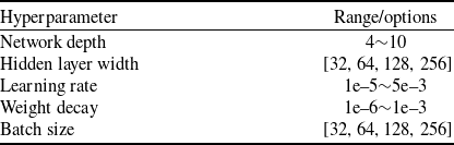
Hyperparameter selection range

Table 1. Long description
The table lists hyperparameter ranges for a machine learning model. It includes the following columns: Hyperparameter and Range/options. The hyperparameters listed are Network depth, Hidden layer width, Learning rate, Weight decay, and Batch size. The ranges or options for each hyperparameter are specified as follows: Network depth ranges from 4 to 10, Hidden layer width options are 32, 64, 128, and 256, Learning rate ranges from 1e-5 to 5e-3, Weight decay ranges from 1e-6 to 1e-3, and Batch size options are 32, 64, 128, and 256.
The hyperparameter ranges in Table 1 were selected based on the low-dimensional nature of the aerodynamic regression problem and the size of the XFoil dataset. To balance model capacity and overfitting risk, the network depth was set to 4–10 residual blocks and the hidden width to [32, 64, 128, 256]. The learning rate (1 × 10⁻⁵−5 × 10⁻³) and weight decay (1 × 10⁻⁶−1 × 10⁻³) were chosen to ensure stable convergence and regularisation, while batch sizes of 32–256 were used to balance training stability and efficiency. Bayesian optimisation was then applied to identify the optimal configuration within these ranges.
4.3 Verification of BO-ARN training effect
BO-ARN training was conducted based on the hyperparameter settings obtained after Bayesian optimisation. To compare the improvement effects of MLP and BO-ARN, Bayesian optimisation was also performed for the hyperparameter selection of the MLP to conduct an ablation experiment.
Root mean square error (RMSE) is introduced as the metric to evaluate the prediction accuracy of the BO-ARN surrogate model. RMSE is defined as the square root of the ratio of the squared deviation between the predicted and true values to the number of predictions n. It is utilised to quantify the average distance between the predicted values and the ground truth (Ground Truth), which can be expressed as:
 \begin{equation}RMSE = \sqrt {\frac{1}{n}\sum\limits_{i = 1}^n {{{({y_{pred,i}} - {y_{true,i}})}^2}} } \end{equation}
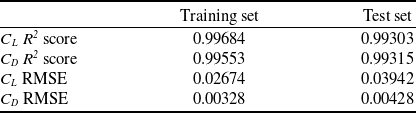
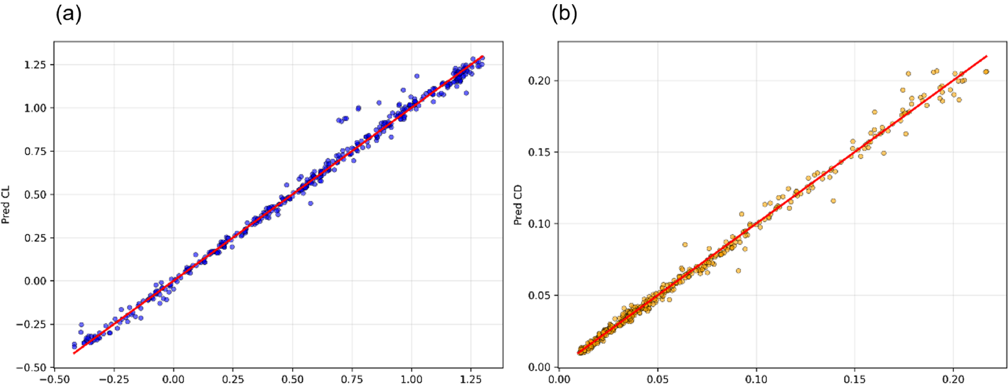
The training results for the MLP and BO-ARN models are obtained as Figs 10 and 11.
MLP training results

Table 2. Long description
A table comparing MLP training results for different metrics. The table has two columns labeled Training set and Test set, and four rows labeled CL R2 score, CD R2 score, CL RMSE, and CD RMSE. Row 1: CL R2 score, 0.99684, 0.99303. Row 2: CD R2 score, 0.99553, 0.99315. Row 3: CL RMSE, 0.02674, 0.03942. Row 4: CD RMSE, 0.00328, 0.00428.
MLP test set R2: (a) test set C L R2 score and (b) test Set C D R2 score.

BO-ARN test set R2: (a) test set C L R2 score and (b) TEST Set C D R2 score.

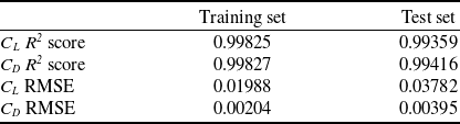
As shown in Tables 2 and 3, the prediction performance of the MLP and BO-ARN models was quantitatively evaluated using the coefficient of determination (R2) and the RMSE. In these tables, C L R2 and C D R2 represent the goodness of fit between the predicted and XFoil-calculated lift and drag coefficients, respectively, while C L RMSE and C D RMSE denote the average prediction errors of lift and drag coefficients, respectively. The training set results reflect the fitting capability of the model, whereas the test set results are used to evaluate its generalisation performance on unseen aerodynamic samples.
BO-ARN training results

Table 3. Long description
A table with two columns labeled Training set and Test set, and four rows labeled CL R2 score, CD R2 score, CL RMSE, and CD RMSE. Row 1: CL R2 score, 0.99825, 0.99359. Row 2: CD R2 score, 0.99827, 0.99416. Row 3: CL RMSE, 0.01988, 0.03782. Row 4: CD RMSE, 0.00204, 0.00395.
Improvement rates of CL and CD RMSE

Table 4. Long description
A table with two columns labeled Training set and Test set, and two rows labeled CL RMSE and CD RMSE. Row 1: CL RMSE, 25.65 percent; 4.06 percent. Row 2: CD RMSE, 37.80 percent; 7.71 percent.
After Bayesian hyperparameter optimisation, both the MLP and BO-ARN models achieved high prediction accuracy. However, compared with the conventional MLP model, the proposed BO-ARN model exhibited better fitting capability and lower prediction errors for both C L and C D . To explicitly quantify this improvement, the RMSE reduction rate of BO-ARN relative to MLP was calculated as:
 \begin{equation}\Delta {\mathrm{RMSE}} = \frac{{{\mathrm{RMS}}{{\mathrm{E}}_{{\mathrm{MLP}}}} - {\mathrm{RMS}}{{\mathrm{E}}_{{\mathrm{BO-ARN}}}}}}{{{\mathrm{RMS}}{{\mathrm{E}}_{{\mathrm{MLP}}}}}} \times 100\% \end{equation}
where
 ${\mathrm{RMS}}{{\mathrm{E}}_{{\mathrm{MLP}}}}$
is the RMSE obtained by the MLP model and
 ${\mathrm{RMS}}{{\mathrm{E}}_{{\mathrm{BO-ARN}}}}$
is the RMSE obtained by the BO-ARN model under the same dataset and evaluation conditions.
The detailed reference values and calculated reduction rates are summarised in Table 4. These results demonstrate that the residual structure significantly improves the nonlinear fitting capability of the network on the training set. Although the improvement on the test set is smaller than that on the training set, BO-ARN still maintains consistently lower errors than MLP, indicating that the enhanced fitting capability does not come at the cost of severe overfitting. This improvement is mainly attributed to the skip-connection mechanism in the residual blocks, which enables the network to learn residual corrections between shallow and deep feature representations and improves gradient propagation during training.
Direct BEMT calculations and BO-ARN-based predictions were performed on the propeller model shown in Fig. 12 (taking a two-bladed propeller operating at an altitude of 25 km, a forward speed of 40 m/s and a rotational speed of 1,200 rpm as an example). The prediction results of BO-ARN for the thrust dT of each blade element segment are close to those of BEMT, demonstrating good predictive performance.
Comparison between BEMT calculation and BO-ARN prediction.

To further evaluate the predictive performance of BO-ARN under different error magnitudes, representative samples were selected based on the percentiles (0%, 25%, 50%, 75% and 100%) of the single-sample RMSEi within the test set. The individual error is defined as follows:
 \begin{equation} RMS{E_i} = \sqrt {\frac{{{{({C_{L,{\mathrm{pred}},i}} - {C_{L,{\mathrm{true}},i}})}^2} + {{({C_{D,{\mathrm{pred}},i}} - {C_{D,{\mathrm{true}},i}})}^2}}}{2}} \end{equation}
where
 ${C_{L,{\mathrm{true}},i}}$
and
 ${C_{D,{\mathrm{true}},i}}$
denote the true lift and drag coefficients of the i-th test sample, respectively, while
 ${C_{L,{\mathrm{pred}},i}}$
and
 ${C_{D,{\mathrm{pred}},i}}$
represent the corresponding model predictions. Re, Mach and
 $\alpha $
correspond to the Reynolds number, Mach number and angle-of-attack for the given sample. As shown in Table 5, the results indicate that BO-ARN maintains high predictive accuracy across most test samples: the RMSE values at the 0%, 25%, 50% and 75% percentiles are 0.0004, 0.0060, 0.0125 and 0.0221, respectively, demonstrating the model’s capability to effectively replicate C
L
and C
D
under typical operating conditions. The maximum error occurs at the 100% percentile sample with an RMSE of 0.1484, which primarily stems from an overestimation of C
L
, whereas the discrepancy in C
D
remains relatively small. Overall, the prediction errors are predominantly concentrated in a few outlying samples, exhibiting robust overall predictive stability.
Comparison of predicted and reference aerodynamic coefficients at representative RMSE percentile positions

Table 5. Long description
A table with seven columns and five rows comparing predicted and reference aerodynamic coefficients at different RMSE percentile positions. The columns are labeled RMSE percentile position, Re, Mach, alpha, RMSE, C L true, C L pred, C D true, and C D pred. The rows present data for RMSE percentile positions at 0 percent, 25 percent, 50 percent, 75 percent, and 100 percent. Each row lists values for Re, Mach, alpha, RMSE, C L true, C L pred, C D true, and C D pred. The table shows variations in these coefficients across different RMSE percentile positions.
Computational cost comparison between BO-ARN BEMT and XFoil BEMT

Table 6. Long description
The table compares the computational cost of two methods, BO-ARN BEMT and XFoil-BEMT. It has two rows and four columns. The columns are labeled Method, Radial sections, Azimuthal points, and Calculation time (s). Row 1: Method, BO-ARN BEMT; Radial sections, 25; Azimuthal points, 180; Calculation time (s), 0.411. Row 2: Method, XFoil-BEMT; Radial sections, 25; Azimuthal points, 180; Calculation time (s), 43.322.
As shown in Table 6, for a single propeller operating condition with 25 radial sections and 180 azimuthal points, the XFoil-supported BEMT method required 43.32 s, whereas the BO-ARN-supported BEMT method required only 0.411 s. This indicates that the proposed neural-network surrogate improves the computational efficiency by approximately 105.4 times.
5.0 Optimisation of propulsion efficiency for high-altitude UAV systems
Since operating conditions severely affect the aerodynamic performance of propellers, the power and system propulsion efficiency of solar-powered UAVs are restricted under the constraints of the motor’s rated parameters. To improve aerodynamic performance, such as thrust and propulsion efficiency under cruise conditions, the rated power and torque of a motor with known performance parameters are used as constraints. This study explores the correlation between the motor and the propeller’s aerodynamic shape matching to enhance propulsion efficiency during cruise and ensure efficient operation of the propeller.
5.1 Optimisation objectives and strategies
Under constraints such as the motor’s rated rotational speed and power, the thrust and propulsion efficiency generated by the initial propeller geometry exhibit clear limitations. To fully utilise the output power of the driving motor and meet the power demands of the propeller under cruise conditions, an optimal design of the propeller’s aerodynamic shape is conducted. The optimisation objective is to maximise the system propulsion efficiency at the design point, with constraints requiring the propeller power to be lower than the motor’s rated power and the propeller torque to be lower than the rated torque. The optimisation problem can be described as:
 \begin{equation}\begin{array}{l}\max \;f(x) = {\eta _{sys}} = {\eta _{prop}} \times {\eta _{motor}}\\s.t.{\mathrm{ }}{P_{shaft}} \le 1000\;W\\{\mathrm{ }}Q \le 8.0\;N \cdot m\end{array}\end{equation}
The system propulsion efficiency is expressed as:
 \begin{equation}{\eta _{sys}} = {\eta _{prop}} \cdot {\eta _{motor}}\end{equation}
The propeller efficiency can be expressed as:
 \begin{equation}{\eta _{prop}} = \frac{{T \cdot V}}{{{P_{shaft}}}}\end{equation}
T is the total thrust produced by the propeller (N), obtained by integrating the BEMT solution; V is the far-field inflow velocity (m/s), which is the flight speed of the UAV. The formula for calculating the propeller power
 ${P_{shaft}}$
(W) (is
 ${P_{shaft}} = Q \cdot \omega $
). Where Q represents the aerodynamic torque of the propeller (N·m);
 $\omega $
represents the propeller’s rotational angular velocity (rad/s). The motor efficiency can be expressed as [Reference McDonald31]:
 \begin{align}{\eta _{motor}} &= \dfrac{{\omega Q}}{{\omega Q + {P_L}}}\nonumber\\[6pt] {P_L} &= {C_0} + {C_1}\omega + {C_2}{\omega ^3} + {C_3}{Q^2}\nonumber\\[6pt] {C_0} &= \dfrac{{\bar \omega \bar Q(1 - \bar \eta )}}{{12\bar \eta }},{C_1} = \dfrac{{ - 3{C_0}}}{{2\bar \omega }} + \dfrac{{\bar Q(1 - \bar \eta )}}{{4\bar \eta }}\\[6pt] {C_2} &= \dfrac{{{C_0}}}{{2{{\bar \omega }^3}}} + \dfrac{{\bar Q(1 - \bar \eta )}}{{4\bar \eta {{\bar \omega }^2}}},{C_3} = \dfrac{{\bar \omega (1 - \bar \eta )}}{{2\bar Q\bar \eta }}\nonumber\end{align}
where
 ${P_L}$
is the power loss (W).
The specific rated parameters of the propeller motor model used in this study are shown in Table 7.
Rated parameters of the propeller motor model

Table 7. Long description
A table showing rated parameters of a propeller motor model. The table has four columns and one row. Column headers are Rated rotational speed/(rad s-1), Rated torque/(N m), Rated efficiency/percent, and Motor rated power/W. Row 1: Rated rotational speed/(rad s-1), 125.664; Rated torque/(N m), 8; Rated efficiency/percent, 90; Motor rated power/W, 1,000.
5.2 Optimisation variables
According to BEMT, the variations in the twist angle and chord length of a propeller are highly correlated with its thrust performance. Consequently, the design variables for optimisation under design point conditions are the radial distributions of chord length C and twist angle
 $\beta$
:
 \begin{equation}Design\;Variable:C,\beta \end{equation}
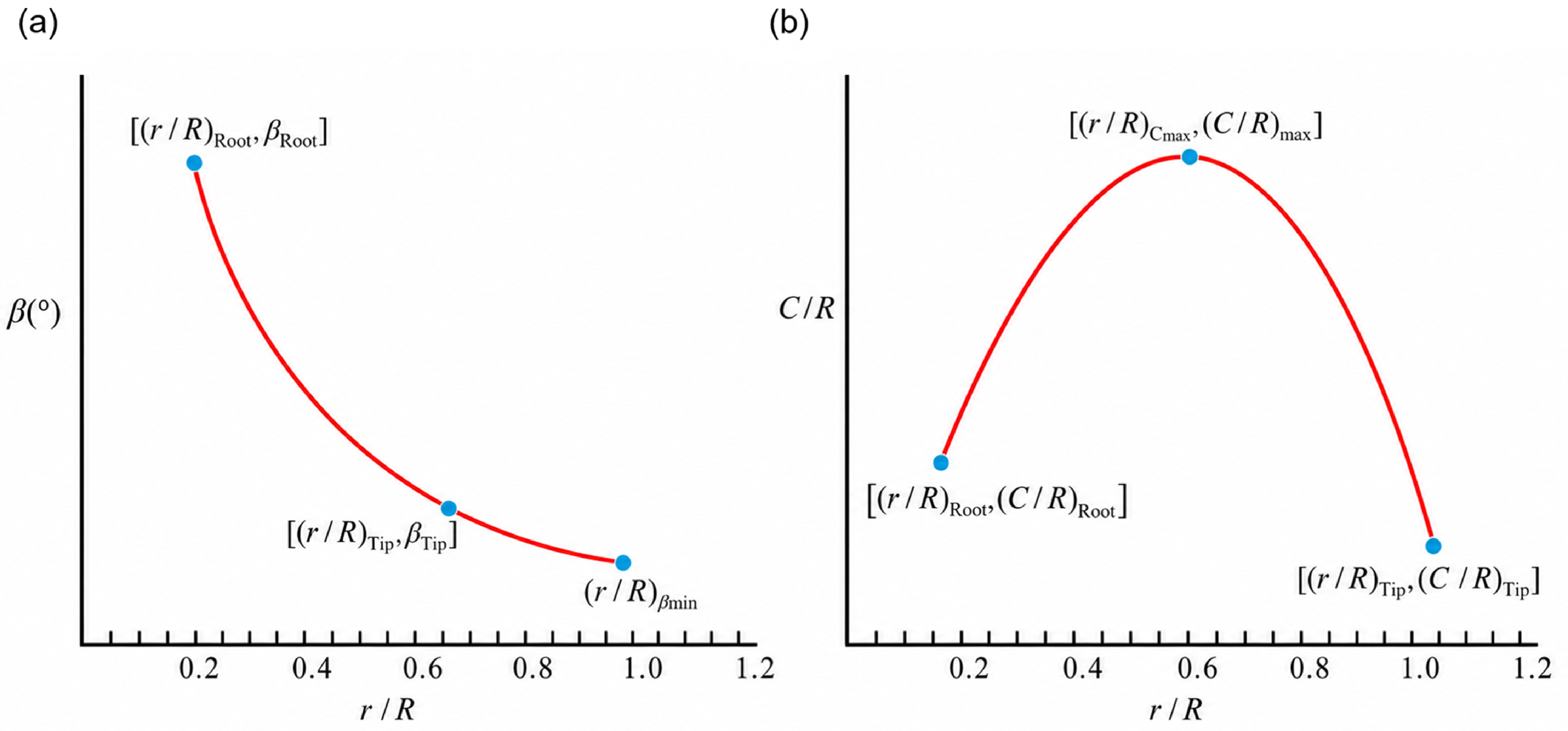
Based on the characteristics of propeller chord distribution, quadratic distribution curves are used to fit the twist angle and chord length of each section along the radial direction to ensure smoothness and continuity. The distribution plots for the twist angle and chord length are shown in Fig. 13.
Distribution diagram of twist angle and chord length: (a) twist-angle distribution and (b) chord-length distribution.

The distribution function is defined as a two-segment quadratic function at the point of maximum chord length. That is, once the extremum of the quadratic function and the coordinates of another point (such as the chord length at the blade root or tip) are known, the quadratic function can be fully determined. Let R denote the propeller radius, C denote the section chord length and
 $\beta$
denote the section twist angle. The coordinates of the maximum chord length point are [
 ${(r/R)_{Cmax}}$
,
 ${(C/R)_{\max }}$
], the coordinates of the chord length at the blade root are [
 ${(r/R)_{Root}}$
,
 ${(C/R)_{Root}}$
], and the coordinates of the chord length at the blade tip are [
 ${(r/R)_{Tip}}$
,
 ${(C/R)_{Tip}}$
]. Then, the chord length distribution can be expressed as:
 \begin{equation}C/R = \left\{ {\begin{array}{*{20}{l}}{{a_1}{{\left[ {r/R - {{(r/R)}_{{C_{\max }}}}} \right]}^2} + {{(C/R)}_{\max }}} {}{r/R \le {{(r/R)}_{{C_{\max }}}}}\\{{a_2}{{\left[ {r/R - {{(r/R)}_{{C_{\max }}}}} \right]}^2} + {{(C/R)}_{\max }}} {}{r/R \gt {{(r/R)}_{{C_{\max }}}}}\end{array}} \right.\end{equation}
 \begin{equation}\begin{array}{l}{a_1} = \dfrac{{{{(C/R)}_{Root}} - {{(C/R)}_{\max }}}}{{{{\left[ {{{(r/R)}_{Root}} - {{(r/R)}_{{C_{\max }}}}} \right]}^2}}}\\[10pt] {a_2} = \dfrac{{{{(C/R)}_{Tip}} - {{(C/R)}_{\max }}}}{{{{\left[ {{{(r/R)}_{Tip}} - {{(r/R)}_{{C_{\max }}}}} \right]}^2}}}\end{array}\end{equation}
The twist angle distribution is also represented by a single quadratic function curve, involving three primary parameters: the twist angle at the blade root section
 ${\beta _{root}}$
, the twist angle at the blade tip section
 ${\beta _{Tip}}$
and the abscissa (x-coordinate) of the function’s extremum
 ${(r/R)_{\beta min}}$
. These parameters uniquely determine a quadratic function:
 \begin{equation}\beta = a{\left[ {r/R - {{(r/R)}_{{\beta _{\min }}}}} \right]^2} + b\end{equation}
 \begin{equation}\begin{array}{l}a = \dfrac{{{\beta _{Root}} - {\beta _{Tip}}}}{{{{\left( {{{(r/R)}_{Root}} - {{(r/R)}_{{\beta _{\min }}}}} \right)}^2} - {{\left( {{{(r/R)}_{Tip}} - {{(r/R)}_{{\beta _{\min }}}}} \right)}^2}}}\\[10pt] b = {\beta _{Root}} - a{\left( {{{(r/R)}_{Root}} - {{(r/R)}_{{\beta _{\min }}}}} \right)^2}\end{array}\end{equation}
The design variables are:
 \begin{align}&Design\ Variable: \nonumber\\ &\mathbf{X}_{\min} \leq \mathbf{X} \leq \mathbf{X}_{\max}\nonumber\\ &\mathbf{X} = \left[ (r/R)_{Cmax}, (C/R)_{max}, (C/R)_{Root}, (C/R)_{Tip}, \beta_{root}, \beta_{tip}, (r/R)_{\beta min}\right]^{T}\end{align}
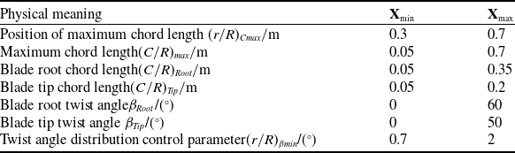
To improve optimisation efficiency and ensure the rationality of the design variables, the constraint ranges of the optimisation variables were further considered within the given geometric parameter limits. The physical meanings and prescribed ranges of the seven optimisation variables are summarised in Table 8. An initial population was randomly generated, with each individual representing a set of propeller geometric design parameters.
5.3 Propeller design point optimisation model
Using BO-ARN as a surrogate model to replace the time-consuming XFoil/CFD iterative calculation process allows for millisecond-level prediction of lift and drag coefficients, which significantly improves optimisation efficiency. The air density (
 $\rho $
), speed of sound (a) and viscosity coefficient (
 $\mu $
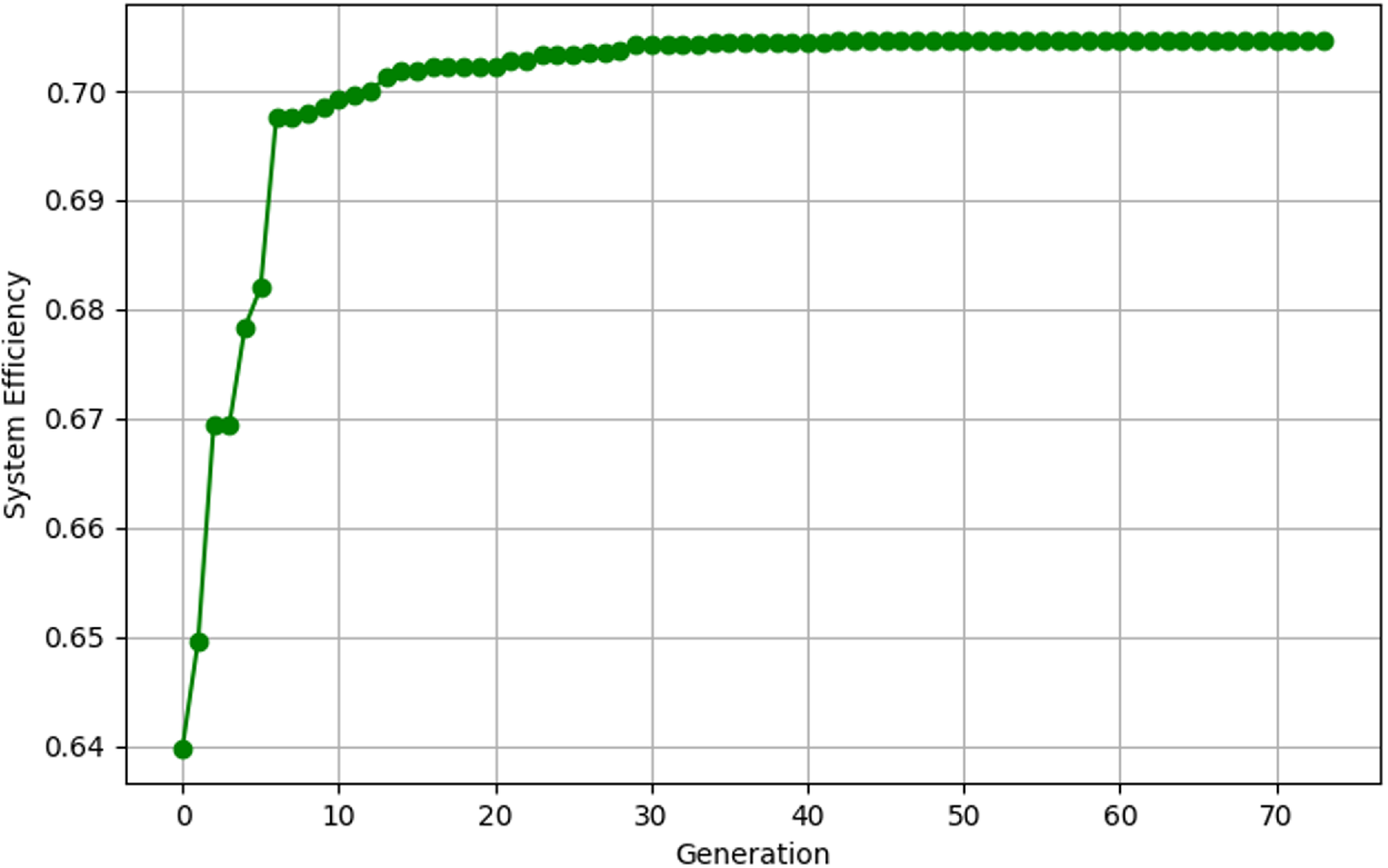
) at the set flight altitude (25 km) are calculated to ensure the physical authenticity of the high-altitude environment simulation. In the process of optimising the propulsion system efficiency, the GA is adopted as the optimisation algorithm to reduce computational resource consumption and improve the efficiency of the iterative process. The parameters for the GA are set with a population size of 200, a maximum of 200 iterations, a crossover probability of 0.8 and a mutation probability of 0.15. An early stopping mechanism is implemented to judge the convergence of the genetic iteration when there is no significant change over 20 generations; the optimisation iteration curve at the design point is shown in Fig. 14.
Ranges of optimisation design variables

Table 8. Long description
A table with two columns and seven rows. The columns are labeled Physical meaning and X with subcolumns Xmin and Xmax. The rows list different design variables and their respective minimum and maximum values. Row 1: Physical meaning, Position of maximum chord length; Xmin, 0.3; Xmax, 0.7. Row 2: Physical meaning, Maximum chord length; Xmin, 0.05; Xmax, 0.7. Row 3: Physical meaning, Blade root chord length; Xmin, 0.05; Xmax, 0.35. Row 4: Physical meaning, Blade tip chord length; Xmin, 0.05; Xmax, 0.2. Row 5: Physical meaning, Blade root twist angle; Xmin, 0; Xmax, 60. Row 6: Physical meaning, Blade tip twist angle; Xmin, 0; Xmax, 50. Row 7: Physical meaning, Twist angle distribution control parameter; Xmin, 0.7; Xmax, 2.
Optimisation iteration curve at the design point.

The optimised design significantly improves the propeller’s thrust and energy conversion efficiency while strictly adhering to the power system constraints. Substituting the results obtained from the surrogate model optimisation back into the BEMT solver revealed that the prediction errors for T and Q were 0.41% and 0.63%, respectively, indicating that BO-ARN possesses considerable precision and achieved excellent results as a surrogate model. As shown in Table 9, the calculated thrust T increased from 17.89 N to 19.49 N,
 ${\eta _{motor}}$
improved from 76.41% to 78.43%, and
 ${\eta _{sys}}$
rose from 68.75% to 70.59%, successfully pushing the design point to the performance boundary and fully utilising the motor and energy system.
5.4 Aerodynamic performance analysis of the optimised propeller
As shown in Fig. 15, the chord and twist-angle distributions are significantly modified after optimisation. For the chord distribution, the optimised blade exhibits a pronounced increase over almost the entire span. The maximum chord appears around the mid-span region (r/R = 0.5), and the optimised chord is substantially larger than that of the initial blade, especially in the range of (r/R = 0.3–0.8). This indicates that the optimisation increases the blade solidity and aerodynamic loading capacity in the main thrust-producing region.
Comparison of various performance parameters before and after optimisation

Table 9. Long description
A table comparing various performance parameters before and after optimization. The table has four rows and six columns. The columns are labeled T/N, Q/(N·m), P_shaft/W, η_motor/%, η_prop/%, and η_sys/%. The rows are labeled Before optimisation, After optimisation, and BEMT. Row 1: Before optimisation, T/N 17.89, Q/(N·m) 7.45, P_shaft/W 936.74, η_motor/% 76.41, η_prop/% 89.98, η_sys/% 68.75. Row 2: After optimisation, T/N 19.57, Q/(N·m) 7.96, P_shaft/W 999.96, η_motor/% 78.30, η_prop/% 90.00, η_sys/% 70.47. Row 3: BEMT, T/N 19.49, Q/(N·m) 7.91, P_shaft/W 994.18, η_motor/% 78.43, η_prop/% 90.00, η_sys/% 70.59.
Comparison of blade geometric parameter distributions before and after optimisation: (a) chord distribution and (b) twist-angle distribution.

In contrast, the twist angle after optimisation is generally lower than that before optimisation, except near the blade root where the two distributions are close. The optimised twist angle decreases more rapidly from the root to the tip and remains lower over most of the span. This reduction in twist angle suggests that the optimised blade weakens excessive local incidence under the cruise condition, improving the matching between blade geometry and inflow velocity.
Overall, the optimised propeller is characterised by a larger chord and a lower twist angle. The increased chord enhances the thrust-generating capability of the middle and outer blade sections, while the reduced twist angle helps control the local angle-of-attack and avoid excessive aerodynamic loading. The coordinated adjustment of chord and twist, therefore, contributes to a more suitable spanwise aerodynamic loading distribution and improves the propeller performance under the design cruise condition.
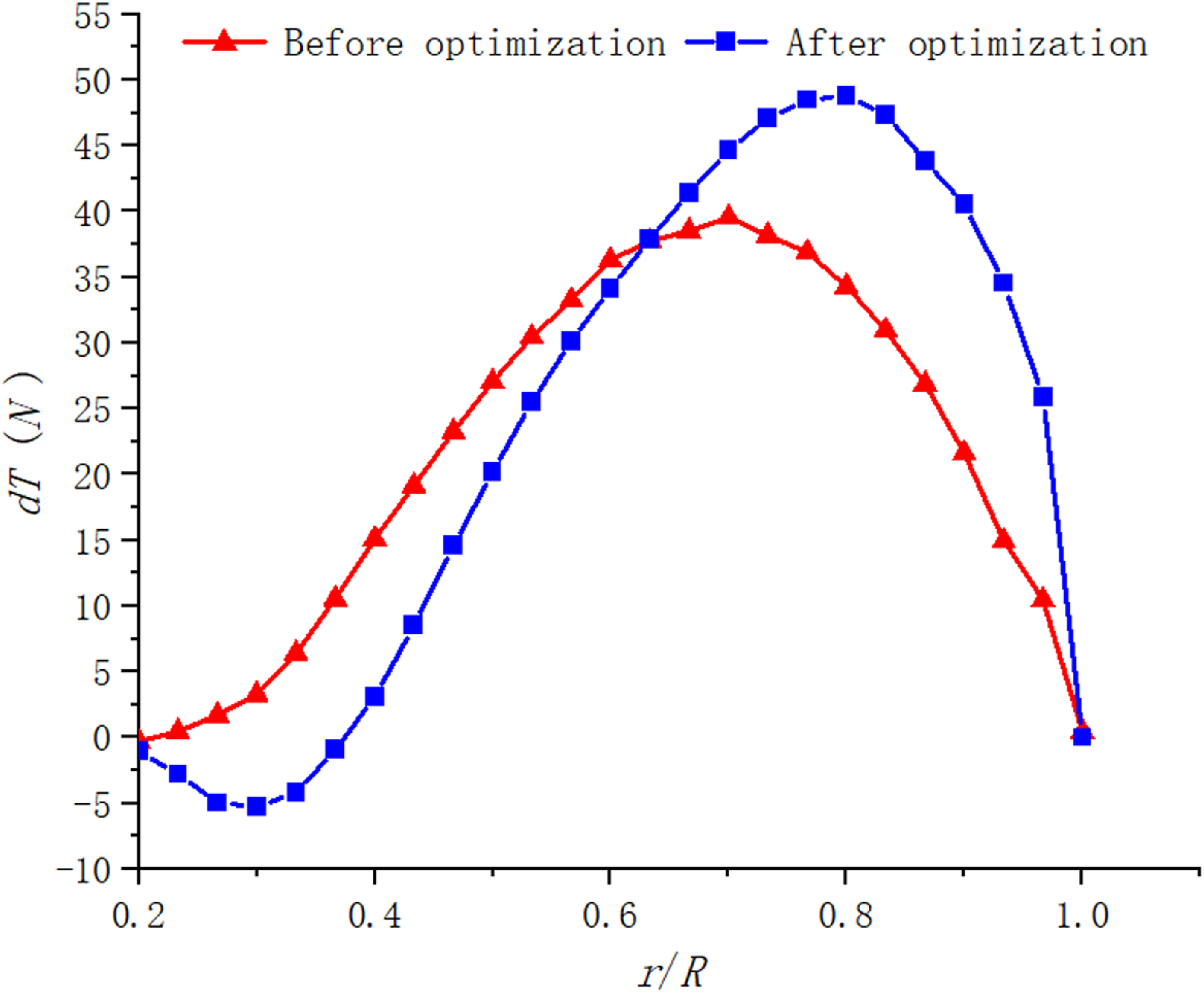
As shown in Fig. 16, the spanwise blade-element thrust distribution is markedly redistributed after optimisation. Before optimisation, the thrust gradually increases from the root to the mid-span region and then decreases toward the blade tip. After optimisation, although a localised negative-thrust region appears near the blade root, the thrust contribution in the middle and outer blade sections is significantly enhanced, and the peak thrust shifts outward. This indicates that the optimised chord and twist distributions strengthen the aerodynamic loading in the main thrust-producing region.
Spanwise distribution of blade element thrust before and after optimisation.

The root negative thrust after optimisation is mainly caused by the local mismatch between inflow angle and blade twist under high-speed cruise conditions. However, because the root region has a small radius and low tangential velocity, its contribution to the total aerodynamic force is limited. In contrast, the middle and outer sections dominate thrust generation due to their higher relative velocity. Therefore, the increased thrust in these effective spanwise regions compensates for the local root loss and leads to an overall improvement in propeller performance.
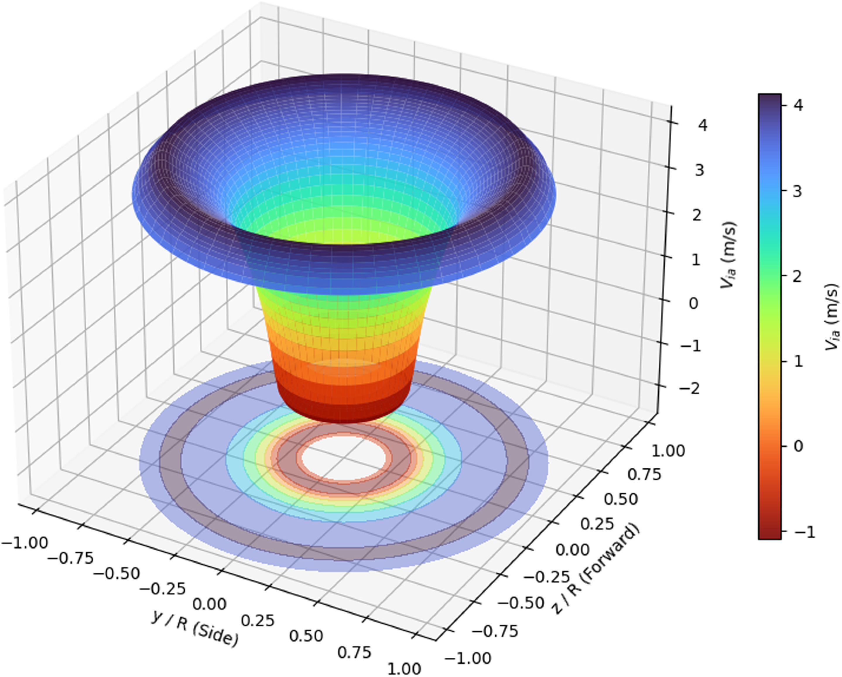
As shown in Fig. 16, the induced velocity distribution further explains this phenomenon. The negative induced velocity near the blade root corresponds to the negative thrust observed in Fig. 17, indicating a local adverse inflow condition in the inner blade region. Nevertheless, after optimisation, the induced velocity and aerodynamic loading in the middle and outer span become more favourable for thrust generation. This redistribution of aerodynamic loading improves the effective utilisation of the blade sections with higher aerodynamic contribution. As a result, the optimised propeller achieves higher total thrust and improved system propulsion efficiency, even though a localised negative-thrust region exists near the blade root.
Induced velocity under high-speed cruise conditions.

6.0 Discussion
The aerodynamic database in this study was constructed from 2,000 LHS samples generated by XFoil for the E387 aerofoil within the prescribed high-altitude, low-Reynolds-number operating range. This sampling strategy was adopted to balance parameter-space coverage, model accuracy, applicable range and database-generation efficiency. Therefore, the present BO-ARN surrogate should be regarded as an interpolation-based model within the sampled Reynolds number, Mach number and angle-of-attack ranges. Its applicability to other aerofoils, different thickness or camber distributions, multi-aerofoil blades or operating conditions outside the training bounds remains to be verified. For broader applicability, additional aerodynamic samples covering extended parameter ranges and aerofoil geometries should be incorporated, followed by model retraining and revalidation.
The fidelity of the database is also limited by XFoil. Although XFoil is efficient for low-speed aerofoil analysis, its accuracy may decrease at very low Reynolds numbers, near stall and at large angles of attack. In particular, when the local Reynolds number approaches or falls below (Re = 10^4), transition, laminar separation bubbles, flow reattachment, strong separation and hysteresis may become highly unsteady and cannot be fully captured by steady two-dimensional polar data. Thus, the optimised design should be interpreted as an engineering optimum under the assumed validity of XFoil-based sectional aerodynamics, rather than a fully generalised optimum for all low-Reynolds-number propeller configurations.
The close agreement between BO-ARN and BEMT indicates that the surrogate model accurately reproduces the XFoil-supported BEMT response and can accelerate repeated aerodynamic evaluations. However, BO-ARN does not capture aerodynamic physics independent of the parent BEMT/XFoil model, and its reliability remains governed by the fidelity of the data-generation process.
GA was adopted because the propeller optimisation problem is nonlinear, constrained and potentially non-convex. Without requiring explicit gradients, GA provides robust global exploration under motor power and torque constraints. The population size and maximum generation number were set to 200, with early stopping applied when no significant improvement occurred over 20 generations. The convergence curve shows that the objective stabilises after approximately 30 generations, indicating that unnecessary iterations were effectively avoided. Nevertheless, PSO, differential evolution and gradient-based surrogate optimisation remain valuable alternatives for future comparison.
The chord and twist distributions were parameterised using quadratic functions to reduce design dimensionality and ensure smooth blade geometries. This improves optimisation robustness but limits the searchable design space; therefore, the obtained optimum represents the best solution within the prescribed quadratic parameterisation rather than a global optimum over all possible blade shapes. More flexible descriptions, such as higher-order polynomials or spline-based parameterisations, should be examined in future work.
The motor–propeller matching model also involves simplification. The system propulsion efficiency was evaluated using a rated or nearly constant motor efficiency, whereas real motors exhibit speed-, torque- and load-dependent efficiency maps. This assumption may affect the ranking of candidate designs near rated power and torque limits. Therefore, the reported efficiency improvement should be further verified using experimentally identified motor efficiency maps.
Overall, this work demonstrates the internal consistency and computational efficiency of a low- to medium-fidelity design workflow, rather than complete physical validation of the final optimised propeller. Although BEMT was compared with available experimental and CFD results, the optimised configuration itself has not yet been independently tested. Future work will extend the aerodynamic database, incorporate higher-fidelity simulations and realistic motor maps, and validate the optimised propeller through wind-tunnel, test-bench or flight experiments.
7.0 Conclusions
Addressing the issues of complex aerodynamic characteristics of HALE solar UAV propellers in the stratospheric low-Reynolds-number environment and the high computational cost of traditional high-fidelity design methods, this paper proposes and validates an efficient aerodynamic shape prediction and optimisation design framework that integrates BEMT, BO-ARN and GA.
-
(1) A high-precision, low-cost surrogate model for aerodynamic characteristic prediction was constructed. Aiming at the strong nonlinear features of aerofoil aerodynamic data at low Reynolds numbers (104–2 × 10⁵), an aerodynamic surrogate model based on ResNet was developed. By introducing Bayesian optimisation (TPE algorithm) for global search of network hyperparameters, the BO-ARN model was successfully established. The research demonstrates that, compared to traditional MLP, the BO-ARN model reduced the RMSE for lift and drag coefficient predictions by 25.65% and 37.80% on the training set, respectively, and by 4.06% and 7.71% on the test set. The model effectively overcomes the degradation problem of deep networks and, while maintaining computational speed, significantly enhances the fitting capability for nonlinear aerodynamic forces in laminar separation and transition zones.
-
(2) System-level optimisation under ‘aero-motor’ coupling constraints was achieved. Based on BEMT theory and the BO-ARN surrogate model, a propeller aerodynamic calculation model was established. Combined with a motor efficiency model, a global optimisation was conducted targeting the system propulsion efficiency under a 25 km cruise condition. Optimisation results show that, under the premise of strictly meeting the engineering constraints of the motor’s rated power (1,000 W) and torque (8 N·m), the performance of the optimised propeller improved significantly: cruise thrust increased from the initial 17.89 N to 19.49 N (an improvement of approximately 8.94%), and the system propulsion efficiency rose from 68.75% to 70.59%.
-
(3) The engineering practicality of the efficient design framework was validated. The accuracy of the theoretical model was verified through a comparison between CFD flow field simulations and BEMT calculation results. The study found that the framework proposed in this paper successfully solves the problems of convergence difficulties and excessive time consumption of traditional methods under low-Reynolds-number and large-twist-angle conditions. The combination of the BO-ARN surrogate model and GA not only achieved refined design of blade chord and twist distribution but also effectively matched the high-efficiency operating range of the motor, providing a rapid and reliable engineering design method for the overall design of high-altitude solar UAV propulsion systems.
In summary, the data-driven propeller optimisation design method proposed in this paper significantly improves the cruise performance of high-altitude propellers while balancing computational efficiency and accuracy. It possesses important theoretical significance and engineering application value for enhancing the long-endurance capabilities of near-space vehicles.
Data availability statement
Some or all data, models or code that support the findings of this study are available from the corresponding author upon reasonable request.
Acknowledgements
The authors would like to thank the School of Aerospace Engineering, Huazhong University of Science and Technology, for providing academic support for this study.
Competing interests
The authors declare that they have no known competing financial interests or personal relationships that could have appeared to influence the work reported in this paper. The authors also declare that they have no non-financial competing interests related to this study.
Financial support
This work is supported in part by funds from the National Natural Science Foundation of China under Grant No. 12172141.
Hardware and software environment
All numerical calculations and neural-network training were performed on a Windows 10 workstation equipped with an AMD64 processor platform and an NVIDIA GeForce RTX 5060 Ti GPU. The software environment was based on Python 3.10.19 and PyTorch 2.10.0 with CUDA 12.8 support.
 η