1. Introduction
Convection through porous media heated from below has captured researchers’ interest because of its intriguing applications in chemical engineering, studying pollutant diffusion in the soil, geophysics, oceanography, CO
 $_2$
sequestration processes, and analogous areas. Such convectional phenomena in porous media are called Rayleigh–Bénard convection. The study of Rayleigh–Bénard convective instability in Newtonian fluids was conducted by Horton & Rogers (Reference Horton and Rogers1945) on horizontal porous surfaces. They determined that
 $4 \pi ^{2}$
was the minimum thermal gradient necessary for the onset of convection. Then Lapwood (Reference Lapwood1948) presented an extended version of the breakdown of stability in a porous layer. This problem is widely recognised as the Horton–Rogers–Lapwood (HRL) problem. Nield & Bejan (Reference Nield and Bejan2006), under certain general assumptions (such as the porous medium being isotropic and homogeneous), made a detailed analysis of the convective stability of Newtonian fluids in a porous layer. Roy & Murthy (Reference Roy and Murthy2017) examined the dissipation effect in a non-Darcy porous medium caused by an inclined temperature gradient. This research article was expanded upon by Dubey & Murthy (Reference Dubey and Murthy2018), who incorporated inclined solutal gradients to study convective instability. The study revealed that the solutal gradient exerts a stabilising influence in the absence of a thermal gradient; in contrast, it demonstrates a destabilising effect in the presence of a thermal gradient. Barletta (Reference Barletta2015) presented proof regarding the possibility of instability of a vertical permeable slab subjected to buoyancy-driven convection. Taking Gill’s instability problem, Shankar & Shivakumara (Reference Shankar and Shivakumara2022) investigated the influence of horizontal permeability of heterogeneity, considering both weak and strong variations. They considered three heterogeneity profiles – linear, quadratic and exponential – to examine linear stability.
Convective instabilities in non-Newtonian fluids exhibit distinctive characteristics that profoundly modify the onset and evolution of flow instability under varying hydrodynamic conditions. Such phenomena are of considerable practical relevance, with applications ranging from enhanced drug bioavailability and optimisation of injection-moulding processes to the prediction and control of blood flow in arterial networks. A wide range of models exists for non-Newtonian fluids, such as Casson, Maxwell, Jeffery, Ellis and power-law fluid models. Each model results in unique and special features that add to its beauty. Barletta & Nield (Reference Barletta and Nield2011) provided a thorough study of the convective stability of non-Newtonian power-law fluids concerning longitudinal and transverse rolls with isothermal boundaries. Alves & Barletta (Reference Alves and Barletta2013) discussed this under Robin’s thermal convective boundary conditions. Various possible models to study linear stability theory have been discussed. Barletta & Storesletten (Reference Barletta and Storesletten2016) discussed the thermal instability of vertical throughflow of the porous media saturated with power-law fluid, where they found that for small throughflow parameters, dilatant fluids are more unstable than pseudo-plastic fluids. Celli et al. (Reference Celli, Barletta, Longo, Chiapponi, Ciriello, Di Federico and Valiani2017) put forward the idea of an open boundary for a power-law fluid in a horizontal porous layer.
Owing to its extensive relevance in geothermal reservoirs, contaminant transport in saturated soils, and food-processing systems, double-diffusive convection arising from the unequal diffusion rates of heat and solute constitutes a fundamental mechanism governing flow instability. Nield (Reference Nield1968) investigated the influence of thermosolutal buoyancy in a horizontal porous layer, employing a Fourier series technique to determine the critical Rayleigh number. His study reveals that thermal and solutal gradients can induce oscillatory instability in the flow system. Charrier-Mojtabi, Elhajjar & Mojtabi (Reference Charrier-Mojtabi, Elhajjar and Mojtabi2007) conducted a study on the Soret mechanism in a binary mixture employing both analytical techniques and numerical simulations. Double-diffusive convective stability under inclined thermal and solutal gradients with thermo-diffusion (the Soret effect) was examined by Narayana, Murthy & Gorla (Reference Narayana, Murthy and Gorla2008), while Wang & Tan (Reference Wang and Tan2011) provided a rigorous analysis of the combined influence of Soret and relaxation-time effects on Maxwell fluid. More recently, Sen et al. (Reference Sen, Roy, Narayana and Kairi2024) advanced this line of inquiry by investigating the double-diffusive instability of a Jeffrey fluid in a porous medium, incorporating vertical throughflow, internal heat generation, and the Soret effect. It is seen from the literature that higher retardation and smaller relaxation time rates were the most destabilising characteristics. Moreover, this reflects the transition of streamlines from unicell to bicell formations in longitudinal rolls.
In the initial stages of research, the researcher overlooked the influence of dissipation in the temperature distribution. Although it was neglected, viscous dissipation has immense significance in natural as well as mixed convection. Gebhart (Reference Gebhart1962) was the first to report the existence of dissipation in natural convection, introducing the Gebhart number to quantify its effect. The Bénard problem under dissipation effect was reported by Turcotte et al. (Reference Turcotte, Hsui, Torrance and Schubert1974). Similarly, other researchers, such as Barletta, Rossi di Schio & Celli (Reference Barletta, Rossi di Schio and Celli2011), have drawn attention to the role of dissipation in horizontal flow between plates within Brinkman’s porous medium. They applied the combined Runge–Kutta and shooting methods to solve the eigenvalue problem. According to Roy, Ponalagusamy & Murthy (Reference Roy, Ponalagusamy and Murthy2020), the behaviour of viscous dissipation in the flow of a viscoelastic fluid through a permeable layer is characterised by the dissipative parameter, which acts in a way that destabilises the flow field. Many authors (Barletta & Celli Reference Barletta and Celli2011; Barletta & Nield Reference Barletta and Nield2012; Roy & Murthy Reference Roy and Murthy2015) have also discussed the implications of viscous dissipation in various situations in detail.
Occasionally, we encounter scenarios where heat is not provided from the base of the porous medium. In that situation, in an HRL problem, a strong internal heat source is introduced to initiate convection. A heat source changes the temperature distribution, which will directly influence the buoyancy forces in thermally driven flows. This change will affect the stability of the system, as increased buoyancy forces could lead to increased instability due to convective motion. Internal heating fundamentally reshapes the basic thermal field, thereby exerting a decisive control on the critical Rayleigh number that dictates the precise threshold for the onset of convection or instability. If the heat source is strong enough, then it can lower the criterion threshold and lead to an earlier onset of convection. Also, in stability analyses, heat sources can raise or lower the amplitudes of disturbances such that they even bring about subcritical bifurcations in which the instability sets in before the usual threshold is attained. Pathiban & Patil (Reference Parthiban and Patil1995) considered pure thermal convection aided by an internal heat source under an inclined temperature gradient. They concluded that transient oscillatory modes would only be possible for small values of the internal heat source, and not for stationary modes. Thereafter, they extended this work to include an anisotropic medium in (Pathiban & Patil Reference Parthiban and Patil1997). Studies on an inclined porous medium with an internal heat source and its stability at isothermal boundary conditions have been performed by Barletta, Celli & Nield (Reference Barletta, Celli and Nield2014). Hill (Reference Hill2005) studied the influence that a concentration-based interior heat source had on the behaviour of double-diffusive convection, while Kumari & Murthy (Reference Kumari and Murthy2019) generalised the concentration heat source regarding the solute diffusion by temperature gradient. The research of Bhadauria (Reference Bhadauria2012) has studied double-diffusive convection in an anisotropic porous layer with an internal heat source. Nouri-Borujerdi et al. (Reference Nouri-Borujerdi, Noghrehabadi and Rees2007) examined a broad collection of theories regarding different temperatures of fluid and solid phases in a uniform heat generation medium. Matta, Narayana & Hill (Reference Matta, Narayana and Hill2016) presented an elaborate description of the thermal instability due to an internal heat source and mass flow through a horizontal porous layer, noticing that the increasing value of the heat source tends to destabilise the flow.
It is noted that instability on thermosolutal convection under contrasting heat sources in a power-law fluid flow through a porous layer has not been examined to date. This study presents a pioneering linear stability analysis of thermosolutal convection in a non-Newtonian power-law fluid saturated within a porous layer, a previously unexplored area. It investigates the interplay of contrasting heat sources and viscous dissipation under permeable isothermal and isosolutal boundary conditions. Novel stability curves are derived to demonstrate how key parameters govern the onset of convective instability. The critical Rayleigh numbers are determined numerically using the Runge–Kutta method coupled with a shooting technique, while flow structures are visualised through streamlines, isotherms and isosolutes for both assisting and opposing buoyancy scenarios.
Physical configuration of the problem.

The findings offer significant insights into controlling instability through flow parameters, understanding non-Newtonian behaviour in porous media, and assessing the impact of viscous dissipation and boundary conditions on flow dynamics. Furthermore, the research highlights substantial practical applications across multiple fields. These include optimising biomedical therapies such as hyperthermia cancer treatment – where the model helps to analyse drug dispersion in tumours – improving industrial processes like chocolate manufacturing, and enhancing the safety assessment of large-scale CO
 $_2$
storage in geological formations.
2. Mathematical model
Consider a horizontal infinite porous layer of height
 $H$
. A non-Newtonian power-law fluid saturates the porous layer with permeable boundary walls at
 $\bar {z} = 0$
and
 $\bar {z} = H$
, as described in figure 1. The medium is assumed to be homogeneous and isotropic, besides being in local thermal equilibrium. At the permeable walls, boundary conditions of temperature and solute concentration are imposed. The contrasting heat source is therefore exchanged between the outside and inside fluid environments at these walls. Take
 $\bar {x}$
and
 $\bar {z}$
in the horizontal and vertical directions of the medium. Usually, temperature and solute concentration are considered as
 $\bar {T}$
and
 $\bar {C}$
, and their differences at the lower and upper boundary walls are
 $\Delta {\bar {T}}\ (\gt 0)$
and
 $\Delta {\bar {C}}\ (\gt 0)$
, respectively. The gravity (
 $\boldsymbol{g}=-g_{0}\hat{\boldsymbol{k}}$
) acts downwards in the negative direction of the
 $\bar {z}$
-axis. The Cartesian components of the seepage velocity
 $\bar {\boldsymbol{u}}$
are denoted by (
 $\bar {u},\bar {v},\bar {w}$
) in the
 $\bar {x}$
,
 $\bar {y}$
and
 $\bar {z}$
directions, respectively.
For the power-law fluid model, the shear stress (
 $\tau$
) is related to the rate of shear strain (
 $\dot {\beta }$
) by
 \begin{equation} \tau = \mu ^{*}(\dot {\beta })^{n} = \mu ^{*}\,|\dot {\beta }|^{n-1}\,\dot {\beta }, \end{equation}
where the terms
 $n$
,
 $\mu ^{*}$
and
 $\mu ^{*}\,|\dot {\beta }|^{n-1}$
are known as the power-law index, the consistency factor, and the apparent viscosity of the fluid, respectively. The power-law index
 $n$
characterises the rheological nature of the fluid. For
 $n=1$
, the fluid behaves as Newtonian, exhibiting a constant viscosity independent of shear rate. When
 $n\lt 1$
, the fluid is pseudo-plastic (shear-thinning), where the apparent viscosity decreases with increasing shear rate, facilitating flow. In contrast, when
 $n\gt 1$
, the fluid is dilatant (shear-thickening), in which the apparent viscosity increases with shear rate, thereby resisting deformation under stronger shear. Since the instability of a flow system is mainly inaugurated by thermosolutal buoyancy differences, the equation of motion for double-diffusive transport phenomena is governed by the generalised Darcy’s law for the power-law fluid model through the porous layer under the linear Oberbeck–Boussinesq approximation given as
 \begin{equation} \frac {{\mu ^*}}{k^*}\,|\bar {\boldsymbol{u}}|^{n-1}\,\bar {\boldsymbol{u}} = -\bar {\boldsymbol{\nabla }}\bar {p} + \rho _{0}g_{0}[\beta _{T}(\bar {T}-T_{0})+\beta _{C}(\bar {C}-C_{0})]\hat {\boldsymbol{k}}. \end{equation}
Here,
 $k^{*} = ({1}/{2c_{t}})( {n\xi ^{\prime }}/({3n +1}))^{n}( {50k}/({3\xi ^{\prime }}))^{( {n+1})/{2}}$
is the generalised permeability of the power-law fluid with intrinsic permeability
 $k$
, porosity
 $\xi ^{\prime }$
,
 $c_{t}$
(
 $={25}/{12}$
) (Christopher & Middleman Reference Christopher and Middleman1965) is the tortuosity factor, and
 $\bar {p}$
is a dynamic pressure. Also,
 $\rho _{0}$
is the fluid density at temperature
 $T_{0}$
and concentration
 $C_{0}$
. The thermal and solutal expansion coefficients are denoted by
 $\beta _{T}$
and
 $\beta _{C}$
, respectively. In the case of Newtonian fluid,
 $ {\mu ^{*}}/{k^{*}} = {\mu }/{k}$
, where
 $\mu$
is called the dynamic viscosity of the Newtonian fluid (
 $n = 1$
).
Under the thermo-solutal convection of the generalised Oberbeck–Boussinesq approximation, incorporating the influence of viscous dissipation and diverse heat source functions, disregarding solute diffusion due to thermal gradients (the Soret effect), the governing equations for the power-law fluid model within the porous medium are formulated as (Hill Reference Hill2005; Barletta et al. Reference Barletta, Rossi di Schio and Celli2011; Barletta & Storesletten Reference Barletta and Storesletten2016; Sen et al. Reference Sen, Roy, Narayana and Kairi2024)
 \begin{align} \bar {\boldsymbol{\nabla }} \boldsymbol{\cdot }{\bar{\boldsymbol{u}}} &= 0, \end{align}
 \begin{align} \frac {{\mu ^*}}{k^*}|{\bar{\boldsymbol{u}}}|^{n-1}{\bar{\boldsymbol{u}}} &= -\bar {\boldsymbol{\nabla }}\bar {p} +\rho _{0}g_{0}[\beta _{T}(\bar {T}-T_{0})+\beta _{C}(\bar {C}-C_{0})]{\hat{\boldsymbol{k}}}, \end{align}
 \begin{align} \sigma \frac {\partial \bar {T}}{\partial \bar {t} }+{\bar{\boldsymbol{u}}}\boldsymbol{\cdot }\bar {\boldsymbol{\nabla }}\bar {T} &= \alpha\, \bar {{\nabla} }^{2}\bar {T}+\frac {\mu ^*}{k^*\rho _{0} c_{p}}|{\bar{\boldsymbol{u}}}|^{n+1} + q_{h}\,F(\bar {z}), \end{align}
 \begin{align} \phi \frac {\partial \bar {C}}{\partial \bar {t}}+{\bar{\boldsymbol{u}}}\boldsymbol{\cdot }\bar {\boldsymbol{\nabla }}\bar {C} &= D\, \bar {{\nabla} }^{2}\bar {C}, \end{align}
where
 $\sigma$
,
 $\alpha$
,
 $\phi$
and
 $D$
stand for the ratio of heat capacities to the volumetric fluid, effective thermal diffusivity, porosity, and mass diffusivity in the porous medium, respectively. Here,
 $g_{0}$
is the reference gravity parameter, and
 $q_{h}$
represents the dimensional heat source parameter with heat source function
 $F(\bar {z})$
.
Profile of various heat source functions.

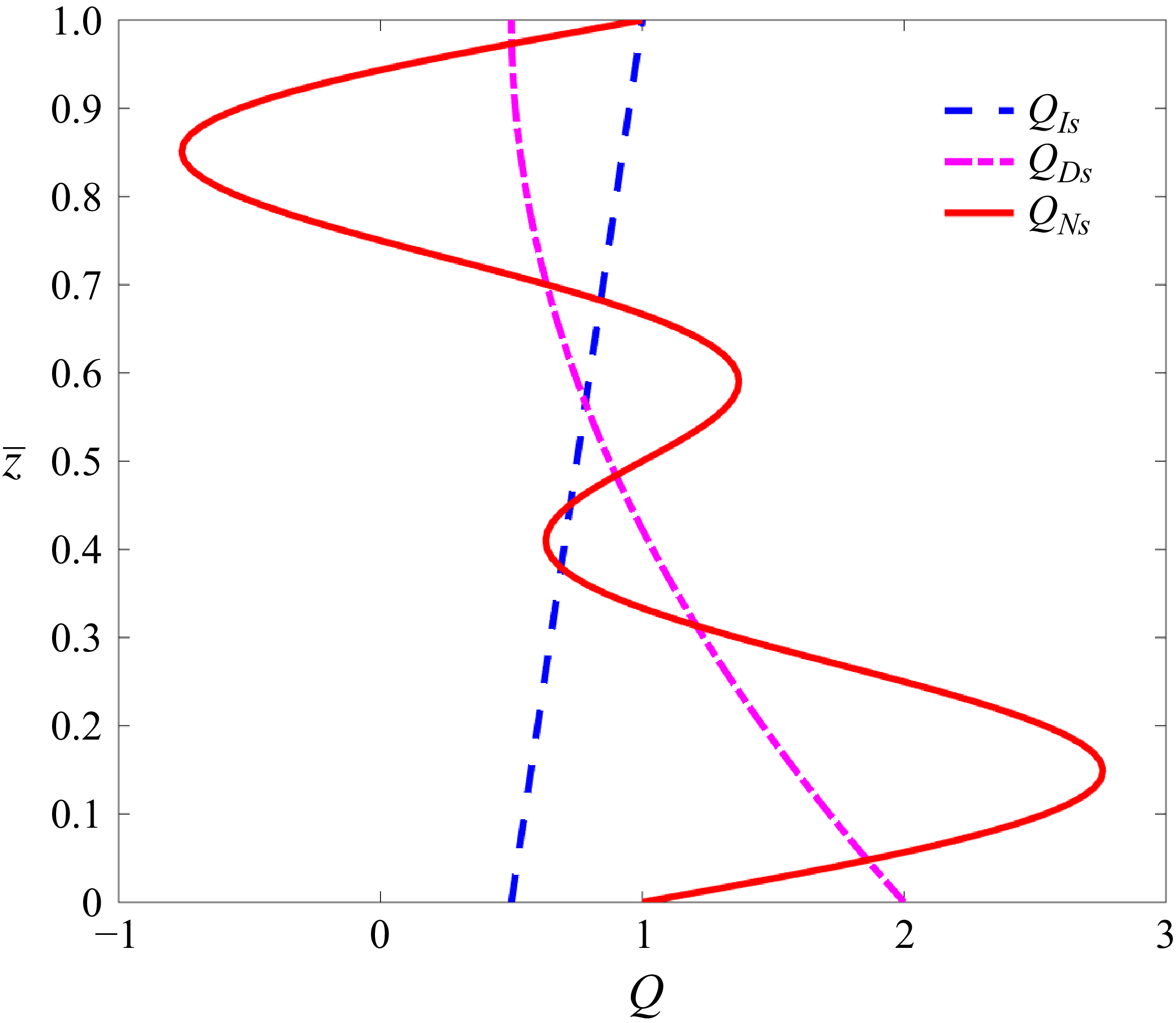
In thermodynamic systems, there are various types of internal heat source functions. Straughan (Reference Straughan1967), the pioneering researcher, was the first to study a uniform heat source. Subsequently, Straughan (Reference Straughan1991, Reference Straughan2003) introduced various internal heat source functions, including exponential, linearly increasing, linearly decreasing and non-uniform, for studying the onset of convection. In our investigation, we considered the following source functions (linearly increasing (
 $Q_{\textit{Is}}$
), linearly decreasing (
 $Q_{\textit{Ds}}$
), and non-uniform (
 $Q_{\textit{Ns}}$
)) (Straughan Reference Straughan2003):
 \begin{align} \text{model}\ Q_{\textit{Is}}\quad F(\bar {z}) &= \left(\frac {1}{2} + \frac {\bar {z}}{H}\right)\!, \end{align}
 \begin{align} \text{model}\ Q_{\textit{Ds}}\quad F(\bar {z}) &= \left(2 + \frac {3}{2}\frac {\bar {z}^{2}}{H^{2}} -\frac {3\bar {z}}{H}\right)\!, \end{align}
 \begin{align} \text{model}\ Q_{\textit{Ns}}\quad F(\bar {z}) &= \left(1 + \sin \frac {2 \pi \bar {z}}{H} + \sin \frac {4 \pi \bar {z}}{H}\right)\!. \end{align}
The beauty of figure 2 encompasses the comprehension of the nature of the various heat source functions. Increasing, decreasing and non-uniform heat source functions are represented by the dashed blue line, the dash-dotted pink line and the solid red line, respectively. As indicated by the dashed blue line labelled
 $Q_{\textit{Is}}$
, the growth of the system continues to increase, hence it is considered an increasing heat source function. A decay of the system denotes a decreasing source function (
 $Q_{\textit{Ds}}$
). Contrary to this, sinusoidal behaviour is seen in the non-uniform heat source function (
 $Q_{\textit{Ns}}$
).
For constant (uniform) vertical throughflow
 $W_{0}$
, the associated boundary conditions are written as (Sen et al. Reference Sen, Roy, Narayana and Kairi2024)
 \begin{eqnarray} && \text{for}\ \bar {z}=0,\quad \bar {w} = W_{0},\ \bar {T} = T_{0} + \Delta {\bar {T}}, \ \bar {C} = C_{0} + \Delta {\bar {C}},\nonumber \\ && \text{for}\ \bar {z}=H,\quad \bar {w}= W_{0},\ \bar {T}= T_{0} , \ \bar {C}= C_{0}. \end{eqnarray}
The dimensional governing equations provided in (2.3a )–(2.3d ) are non-dimensionalised through the variables (Roy & Murthy Reference Roy and Murthy2016; Dubey & Murthy Reference Dubey and Murthy2018):
 \begin{eqnarray} &&\frac {1}{H}(\bar {x},\bar {y},\bar {z})\rightarrow \boldsymbol{x},\quad \frac {H}{\alpha }(\bar {u},\bar {v},\bar {w})\rightarrow \boldsymbol{u}, \quad\frac {\alpha }{\sigma H^{2}}\bar {t}\rightarrow t,\nonumber \\ &&\frac {\bar {T}-T_{0}}{\Delta {\bar {T}}}\rightarrow T,\quad H\bar {\boldsymbol{\nabla }} \rightarrow \boldsymbol{\nabla },\quad H^{2}\bar {\nabla} ^{2} \rightarrow {\nabla} ^{2},\quad\frac {\bar {C}-C_{0}}{\Delta \bar {C}} \rightarrow C. \end{eqnarray}
After non-dimensionalising, applying the curl operator to both sides of (2.3b ), and eliminating the pressure gradient from the equation of motion, the resulting modified governing equations are obtained as
 \begin{align} \boldsymbol{\nabla }\boldsymbol{\cdot }\boldsymbol{u} &= 0 , \end{align}
 \begin{align} \boldsymbol{\nabla }\times |\boldsymbol{{u}}|^{n-1}\boldsymbol{{u}} &= {\textit{Ra}} \,\boldsymbol{\nabla }\times \left [(T + N C){\hat{\boldsymbol{k}}}\right ], \end{align}
 \begin{align} \frac {\partial T}{\partial t} + \boldsymbol{u}\boldsymbol{\cdot }\boldsymbol{\nabla }T &= {\nabla} ^{2}T +\frac {\textit{Ge}}{\textit{Ra}}|\boldsymbol{{u}}|^{n+1}+ Q\,F(z) , \end{align}
 \begin{align} \varLambda \frac {\partial C}{\partial t} + \boldsymbol{u}\boldsymbol{\cdot }\boldsymbol{\nabla }C &= \frac {1}{\textit{Le}}{\nabla} ^{2}C, \end{align}
with the boundary conditions given by
 \begin{eqnarray} && \text{for}\ z = 0,\quad w = \textit{Pe},\ T= 1,\ C= 1,\nonumber \\&& \text{for}\ z = 1,\quad w = \textit{Pe},\ T= 0,\ C = 0, \end{eqnarray}
where the dimensionless parameter
 ${\textit{Ra}} = {\rho _{0} g_{0}\beta _{T}\,\Delta {\bar {T}}\, k^* H^n}/({\mu ^* \alpha ^{n}})$
is considered as the non-Newtonian Rayleigh number, and
 $N = (\beta _{C}\,\Delta {\bar {C}})/({\beta _{T}\,\Delta {\bar {T}}})$
is the ratio of solutal and thermal buoyancy forces in a porous medium. In aiding buoyancy (solutal and thermal buoyancy forces act in the same direction) and in opposing buoyancy (solutal and thermal buoyancy forces act in opposite directions),
 $N$
is considered as
 $\gt 0$
and
 $\lt 0$
, respectively. Here,
 $\textit{Pe} = {W_{0}H}/{\alpha }$
represents the Péclet number,
 $Le = {\alpha }/{D}$
is the Lewis number, and
 $\varLambda = {\phi }/{\sigma }$
. The internal heat parameter
 $Q$
is defined by
 $({H^{2}}/({\alpha\, \Delta {\bar {T}}}))q_{h}$
with heat source function
 $F(z)$
. The Gebhart number
 $\textit{Ge}$
is expressed as
 $ {g_0 \beta _{T}H}/{c_p}$
.
Basic temperature distribution at different states of the heat source under the influence of vertical throughflow, when
 $n=0.5,\ Ra=100$
and
 $\textit{Ge}=1.0$
.

Basic concentration distributions at different states of the diffusivity ratio under the influence of vertical throughflow.

2.1. Basic steady-state flow
Assuming a base flow in the vertical
 $z$
-direction with purely vertical temperature and concentration gradients, a fully developed unidirectional flow leads to a steady-state solution with the following boundary conditions:
 \begin{align}&\qquad\qquad\qquad\qquad\qquad u_{b} = 0,\,\,\,\,\,\,v_{b}= 0,\,\,\,\,\,\,w_{b} = \textit{Pe}, \end{align}
 \begin{align}&\qquad\qquad\qquad\qquad\qquad\qquad C_{b} =\frac {\textrm{e}^{\textit{Le}\,\textit{Pe}}-\textrm{e}^{\textit{Le}\,\textit{Pe}\,z}}{\textrm{e}^{\textit{Le}\,\textit{Pe}}-1}, \end{align}
 \begin{align} T_{b} &= \frac {1}{\textrm{e}^{{\textit{Pe}}}-1} \Biggl [ \int _1^z \textrm{e}^{{\textit{Pe}}\, \xi } \Biggl ( (\textrm{e}^{{\textit{Pe}}}-1) \int _1^{\xi } -\frac {\textrm{e}^{-{\textit{Pe}}\, \delta } \left (Q \, {\textit{Ra}}\, F(\delta )+{\textit{Ge}} \, {\textit{Pe}}^{n+1}\right )}{{\textit{Ra}}} \, {\rm d}\delta \nonumber \\ &\quad {}+ {\textit{Pe}}\, \Biggl ( \int _1^0 \textrm{e}^{{\textit{Pe}}\, \xi } \int _1^{\xi } -\frac {\textrm{e}^{-{\textit{Pe}}\, \delta } \left (Q \, {\textit{Ra}}\, F(\delta )+{\textit{Ge}} \, {\textit{Pe}}^{n+1}\right )}{{\textit{Ra}}} \, {\rm d}\delta \, {\rm d}\xi - 1 \Biggr ) \Biggr ) \, {\rm d}\xi \Biggr ]. \end{align}
Figure 3(a–c) depict the variation of the basic temperature distribution under different heat source conditions in the presence of vertical throughflow. It is observed that with increasing throughflow, the basic thermal profile evolves consistently across all source states. Significantly, a higher heat source parameter (
 $Q$
) strengthens the temperature profile. However, the improvement is mostly observed for non-uniform source functions.The non-uniform heat source delivers more energy to certain regions, resulting in an enhanced temperature profile. Figure 4(a,b) indicate an increase in solute concentration as flows move at large flow shear rates. But not much intensity is given to the throughflow at
 $Le=0.5$
. Physically, the diffusivity ratio (
 ${\textit{Le}}$
) depicts the ratio of thermal diffusivity to solutal diffusivity. Therefore,
 $Le=0.5\lt 1$
means higher solutal diffusivity, i.e. the diffusion rate of concentration is much faster; hence the effect of
 $\textit{Pe}$
is small. On the other hand, when
 $Le=10\gt 1$
, the solutal diffusivity is relatively low, which enhances the influence of throughflow on the system.
2.2. Linear instability analysis
To study the linear instability of the basic flow against small disturbances, we introduce small perturbations to the basic solution such that
 \begin{eqnarray} \boldsymbol{u} =\boldsymbol{u}_{b} +\epsilon {\hat{\boldsymbol{u}}},\quad T = T_{b} +\epsilon \hat {\tau }, \quad C = C_{b} +\epsilon \hat {\varTheta }, \end{eqnarray}
where
 $\epsilon \ll 1$
is a small perturbation parameter, and
 ${\hat{\boldsymbol{u}}}$
,
 $\hat {\tau }$
and
 $\hat {\varTheta }$
are infinitesimal disturbances in velocity, temperature and concentration, respectively. By plugging (2.14) into (2.9)–(2.10), and neglecting
 $O(\epsilon ^2)$
terms, the following perturbation equations and boundary conditions are obtained:
 \begin{align} &\qquad\qquad\qquad\qquad\qquad \left(\frac {\partial \hat {u}}{\partial x} + \frac {\partial \hat {v}}{\partial y} + \frac {\partial \hat {w}}{\partial z}\right) = 0 , \end{align}
 \begin{align} &\qquad\qquad \left(n\frac {\partial \hat {w}}{\partial y} - \frac {\partial \hat {v}}{\partial z}\right)= \frac {\textit{Ra}}{|\textit{Pe}|^{n-1}}\left (\frac {\partial \hat {\tau }}{\partial y} + N\frac {\partial \hat {\varTheta }}{\partial y}\right )\!, \end{align}
 \begin{align} &\qquad\qquad \left(n\frac {\partial \hat {w}}{\partial x} - \frac {\partial \hat {u}}{\partial z}\right) =\frac {\textit{Ra}}{|\textit{Pe}|^{n-1}} \left (\frac {\partial \hat {\tau }}{\partial x} +N\frac {\partial \hat {\varTheta }}{\partial x}\right )\!, \end{align}
 \begin{align} & \left(\frac {\partial \hat {\tau }}{\partial t} + \textit{Pe}\frac {\partial \hat {\tau }}{\partial z} + \hat {w}\frac {{\rm d}T_{b}}{{\rm d}z}\right) = \left (\frac {\partial ^2 \hat {\tau }}{\partial {x^2}} + \frac {\partial ^2 \hat {\tau }}{\partial {y^2}} + \frac {\partial ^2 \hat {\tau }}{\partial {z^2}}\right )+\frac {\textit{Ge}}{\textit{Ra}}(n+1)\,P\textrm{e}^{n}\,\hat {w}, \end{align}
 \begin{align} &\qquad \left(\varLambda \frac {\partial \hat {\varTheta }}{\partial t} + \textit{Pe}\frac {\partial \hat {\varTheta }}{\partial z} + \hat {w}\frac {{\rm d}C_{b}}{{\rm d}z}\right) =\frac {1}{\textit{Le}}\left ( \frac {\partial ^2 \hat {\varTheta }}{\partial {x^2}} + \frac {\partial ^2 \hat {\varTheta }}{\partial {y^2}} + \frac {\partial ^2 \hat {\varTheta }}{\partial {z^2}}\right )\!, \end{align}
 \begin{align} &\qquad\qquad\qquad\qquad \text{for} \ z = 0,\quad\hat {w} = 0,\ \hat {\tau } = 0, \ \hat {\varTheta } = 0, \end{align}
 \begin{align} &\qquad\qquad\qquad\qquad \text{for} \ z = 1,\quad \hat {w} = 0,\ \hat {\tau } = 0, \ \hat {\varTheta } = 0. \end{align}
Upon differentiating (2.15b
) with respect to
 $y$
, and (2.15c
) with respect to
 $x$
, and subsequently adding the two equations, one may, with the aid of (2.15a
) and by invoking wave-like disturbances
 $(\hat {w}, \hat {\tau }, \hat {\varTheta }) = (W(z), \theta (z), \kappa (z))\, \textrm{e}^{ia_{x}x +ia_{y}y+\eta t}$
(Kumari & Murthy Reference Kumari and Murthy2018) corresponding to the neutrally stable mode, obtain the relations
 \begin{align} &\qquad\,\, W^{\prime \prime } - a^{2}n W + a^2 \frac {\textit{Ra}}{|\textit{Pe}|^{n-1}}\left (\theta + N \kappa \right ) = 0, \end{align}
 \begin{align} & \theta ^{\prime \prime } -\textit{Pe}\,\theta ^{\prime } -a^{2}\theta - L(z)\, W+ \frac {\textit{Ge}}{\textit{Ra}}(n+1)\,P\textrm{e}^n\, W = 0, \end{align}
 \begin{align} &\qquad\quad \kappa ^{\prime \prime } -\textit{Le}\,\textit{Pe}\,\kappa ^{\prime }- a^{2}\kappa - Le\,W\,I(z) = 0, \end{align}
 \begin{align} &\qquad\qquad \text{for} \ z = 0,\quad W = 0,\ {\theta } = 0, \ \kappa = 0, \end{align}
 \begin{align} &\qquad\qquad \text{for} \ z = 1,\quad W = 0,\ {\theta } = 0, \ \kappa = 0, \end{align}
 \begin{align} &\qquad\qquad\qquad \textit{where}\quad a= \sqrt {a_{x}^2+a_{y}^2}. \end{align}
2.3. Stream function approach
Define the stream function
 $\psi$
as
 $\hat {u} = {\partial \psi }/{\partial z}$
and
 $\hat {w} = - ( {\partial \psi }/{\partial x})$
. The system of partial differential equations and boundary conditions can then be written as follows:
 \begin{align} &\qquad\qquad \left (n\frac {\partial ^2 \psi }{\partial x^2} + \frac {\partial ^2 \psi }{\partial z^2} \right )+ \frac {\textit{Ra}}{|\textit{Pe}|^{n-1}}\left (\frac {\partial \hat {\tau }}{\partial x} + N\frac {\partial \hat {\varTheta }}{\partial x}\right ) = 0, \end{align}
 \begin{align} & \left (\frac {\partial \hat {\tau }}{\partial t} + \textit{Pe}\frac {\partial \hat {\tau }}{\partial z} - \frac {\partial \psi }{\partial x}\frac {{\rm d}T_{b}}{{\rm d}z}\right ) - \left (\frac {\partial ^2 \hat {\tau }}{\partial {x^2}} + \frac {\partial ^2 \hat {\tau }}{\partial {y^2}} + \frac {\partial ^2 \hat {\tau }}{\partial {z^2}}\right )+\frac {\textit{Ge}}{\textit{Ra}}\left (n+1\right )P\textrm{e}^{n}\frac {\partial \psi }{\partial x} = 0, \end{align}
 \begin{align} &\qquad \left (\varLambda \frac {\partial \hat {\varTheta }}{\partial t} + \textit{Pe}\frac {\partial \hat {\varTheta }}{\partial z} - \frac {\partial \psi }{\partial x}\frac {{\rm d}C_{b}}{{\rm d}z}\right ) -\frac {1}{\textit{Le}}\left ( \frac {\partial ^2 \hat {\varTheta }}{\partial {x^2}} + \frac {\partial ^2 \hat {\varTheta }}{\partial {y^2}} + \frac {\partial ^2 \hat {\varTheta }}{\partial {z^2}}\right ) = 0, \end{align}
 \begin{align} &\qquad\qquad\qquad\qquad \text{for} \ z = 0,\quad \frac {\partial \psi }{\partial x} = 0,\ \hat {\tau } = 0, \ \hat {\varTheta } = 0, \end{align}
 \begin{align} &\qquad\qquad\qquad\qquad \text{for} \ z = 1,\quad \frac {\partial \psi }{\partial x} = 0,\ \hat {\tau } = 0, \ \hat {\varTheta } = 0. \end{align}
The neutral or marginal instability of a system is characterised using the normal mode approach (Roy & Murthy Reference Roy and Murthy2015; Kumari & Murthy Reference Kumari and Murthy2018),
 \begin{eqnarray} \psi =\big (i\,W(z)\, \textrm{e}^{{\rm i}ax+\eta t}\big),\quad\hat {\tau } = \big(\theta (z)\, \textrm{e}^{{\rm i}ax+\eta t}\big), \quad\hat {\varTheta } = Le\,\big(\kappa (z)\, \textrm{e}^{{\rm i}ax+\eta t}\big), \end{eqnarray}
where the parameter
 $a$
is the wavenumber, and
 $\eta$
is complex; its real part is the growth rate of the disturbance, while its imaginary part describes the angular frequency. Now, substituting (2.27) into (2.24)–(2.26), we derive the system of eigenvalue problems for the neutral stability modes (
 $\eta =0$
) (Barletta & Storesletten Reference Barletta and Storesletten2016):
 \begin{align} &\qquad\,\, W^{\prime \prime } - a^{2}n W + a \frac {\textit{Ra}}{|\textit{Pe}|^{n-1}}\left (\theta + N\, Le\, \kappa \right ) = 0, \end{align}
 \begin{align} & \theta ^{\prime \prime } -\textit{Pe}\,\theta ^{\prime } -a^{2}\theta - a\,L(z)\, W+a \frac {\textit{Ge}}{\textit{Ra}}(n+1)\,\textit{Pe}^n\, W = 0, \end{align}
 \begin{align} &\qquad\quad\,\, \kappa ^{\prime \prime } -Le\,\textit{Pe}\,\kappa ^{\prime }- a^{2}\kappa - a\,W\,I(z) = 0, \end{align}
 \begin{align} &\qquad\qquad \text{for} \ z = 0,\quad W = 0,\ {\theta } = 0, \ \kappa = 0, \end{align}
 \begin{align} &\qquad\qquad \text{for} \ z = 1,\quad W = 0,\ {\theta } = 0, \ \kappa = 0. \end{align}
2.4. Numerical procedure
The system of coupled ordinary differential equations along with boundary conditions given in (2.28)–(2.32) constitutes an eigenvalue problem with
 ${\textit{Ra}}$
serving as the eigenvalue. Such systems are efficiently solved numerically by combining the use of sixth-order Runge–Kutta (function NDSolve) with the shooting technique (function FindRoot) in the Mathematica 14.0 software package (@Wolfram, Inc.). In fact, the Runge–Kutta procedure is employed to transform boundary value problems into initial value problems. Now the modified initial conditions for
 $z=0$
can be written as
 \begin{eqnarray} &\text{for} \ z = 0,\quad W = 0,\ W' =1,\ \theta = 0, \ \theta ^{\prime } = \zeta _{1}, \ \kappa = 0, \ \kappa ' = \zeta _{2}. \end{eqnarray}
In other words, this method is used as a solution procedure for an initial value problem. To normalise the disturbance scale of the system, the condition
 $W^{\prime } (0) = 1$
is established, and the missing initial conditions are consequently calculated by means of the guessed values
 $\zeta _{1}$
and
 $\zeta _{2}$
. This job is done by the shooting method. After solving the initial value problem, the eigenvalue is found, denoted by
 ${\textit{Ra}}$
. Additionally, the components
 $\zeta _{1}$
and
 $\zeta _{2}$
are obtained with the help of the boundary condition
 $z=1$
for each given set of parameters (
 $a, n, N, Le, Ge, \textit{Pe}, Q$
). After finding the Rayleigh number
 ${\textit{Ra}}$
as a function of the wavenumber
 $a$
, i.e.
 ${\textit{Ra}}(a)$
for every prescribed value of the parameters, the critical values of the pair
 $(Ra_{c}, a_{c})$
are obtained by minimising the function
 ${\textit{Ra}}(a)$
to identify the onset of instability.
2.5. Validation
The investigation establishes various outcomes on vertical throughflow for linear instability analysis of power-law fluid through the porous medium under suitable parametric influence. These findings are presented through plots of the critical Rayleigh number
 ${\textit{Ra}}_{c}$
as a function of different controlling parameters, which effectively capture the transition between stable and unstable flow regimes. For numerical investigation, the physical ranges of parameters are taken as
 $0\lt n\leqslant 2$
(Alves & Barletta Reference Alves and Barletta2013),
 $0\lt \textit{Pe}\leqslant 2$
(Barletta & Storesletten Reference Barletta and Storesletten2016),
 $0\lt \textit{Ge}\leqslant 1$
(Roy & Murthy Reference Roy and Murthy2015),
 $0\leqslant Q\leqslant 5$
(Sen et al. Reference Sen, Roy, Narayana and Kairi2024),
 $-1\lt N\leqslant 1$
(Kumari & Murthy Reference Kumari and Murthy2018), and
 $0\lt Le\leqslant 10$
(Narayana et al. Reference Narayana, Murthy and Gorla2008). For the case of pure thermal convection (
 $N=0$
), in the absence of vertical throughflow (
 $\textit{Pe}=0$
), heat source parameter (
 $Q=0$
) and viscous dissipation (
 $\textit{Ge}=0$
), the present analysis shows excellent agreement with the benchmark results of Barletta & Nield (Reference Barletta and Nield2011). In the limiting case
 $\textit{Pe}\to 0$
(
 $\textit{Pe}=10^{-4}$
), the critical Rayleigh number at the onset of convection is obtained as
 ${\textit{Ra}}_{c}=5.75\times 10^{-3}$
, with the corresponding wavenumber
 $a_{c}=2.64$
for a dilatant fluid (
 $n=2$
), and
 ${\textit{Ra}}_{c}=2.88\times 10^{3}$
with
 $a_{c}=3.74$
for a pseudo-plastic fluid (
 $n=0.5$
). For the Newtonian case (
 $n=1$
), the present computation yields
 ${\textit{Ra}}_{c}=39.48$
at
 $a_{c}=3.14$
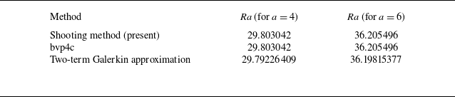
, evaluated using a Runge–Kutta integration coupled with a shooting technique in Mathematica 14.0. This number corresponds really well to an accepted datum by Barletta & Nield (Reference Barletta and Nield2011), in particular, adhering to the analytical solution presented in their equation (43). Such equality can be invoked to justify the computational method of pursuit here and also confirm the strength of using Runge–Kutta integration alongside the shooting technique. The ability of the current formulation to reproduce the already established threshold values of the critical Rayleigh numbers and their corresponding wavenumbers for thermal convection across the dilatant rheological model, pseudo-plastic rheological models and Newtonian rheological models presents ample evidence that the present formulation is indeed dependable for detecting the onset conditions of thermal convection. Thus having good agreement with Barletta & Nield (Reference Barletta and Nield2011) confirms that the numerical scheme has been implemented very accurately and that the stability thresholds derived are consistent with the literature. Also, using a different methodology for pure thermal convection with vertical throughflow, the present results are found to be in good agreement with those reported by Kumari & Murthy (Reference Kumari and Murthy2018), as shown in table 1.
Comparison of results obtained by Kumari & Murthy (Reference Kumari and Murthy2018) using the bvp4c and Galerkin approximation with present results using the shooting method coupled with the Runge–Kutta solver with adaptive step size for
 $N=0$
,
 $\textit{Ge}=Q=0$
,
 $n=0.5$
and
 $\textit{Pe}=1$
.

Effect of
 $\textit{Pe}$
on
 ${\textit{Ra}}_{c}$
for various heat source functions in (a) aiding buoyancy (
 $N=1.0$
), (b) opposing buoyancy (
 $N=-0.1$
), at
 $Q = 1$
,
 $\textit{Ge} = 0.01$
and
 $Le = 1$
.

3. Results and discussion
3.1.
Parametric control of
 ${\textit{Ra}}_{c}$

The impact of vertical throughflow on the onset of instability of non-Newtonian power-law fluid through the porous layer is depicted in figure 5(a,b) for different kinds of heat source functions (such as increasing, decreasing and non-uniform) in aiding and opposing buoyancies. From figure 5(a), the response of Péclet number (
 $\textit{Pe}$
) on critical thermal Rayleigh number (
 ${\textit{Ra}}_{c}$
) for various heat source functions in the aiding buoyancy case is displayed for various values of
 $n$
with fixed
 $Q, \textit{Ge}, Le$
. It is revealed from figure 5(a) that the smaller shear rate flow executes infinite apparent viscosity of pseudo-plastic fluid (i.e.
 $n \lt 1$
) as a result of
 ${\textit{Ra}}_{c}$
decreases for small
 $\textit{Pe}$
, leading to a destabilised flow zone under various heating in the porous layer. But under dilatant fluid conditions where
 $n=2$
, at a very low shear rate, there will be negligible apparent viscosity, and this condition will fetch an extremely stabilised region concerned with the flow system. At large shear rates, the stabilising influence becomes markedly stronger for
 $n\geqslant 1$
, whereas the destabilising tendency is overwhelmingly pronounced for
 $n\lt 1$
. Consequently, a strong throughflow exerts a dominant and decisive impact on the stability characteristics across all values of the power-law index
 $n$
. In the opposing buoyancy scenario (figure 5
b), a similar effect is observed, as in aiding here the critical Rayleigh number
 ${\textit{Ra}}_{c}$
rises substantially compared to the aiding case. Since thermal and solutal buoyancy forces act in the same direction for aiding buoyancy, they reinforce each other and thereby tend to reduce the threshold required for the initiation of the stability. This is why
 ${\textit{Ra}}_{c}$
remains relatively low. In opposing buoyancy, the solutal buoyancy force opposes the thermal buoyancy. Hence two driving mechanisms come into competition. In fact, convection is hindered by the solute-induced density gradient, which is contrary to the destabilising effect due to the thermal field. Generally, instability develops when the destabilising buoyancy is higher (thermal) than the stabilising buoyancies of viscous dissipation, diffusion or solutal action. In the opposite case, the system will be expected to be subjected to much greater thermal buoyancy in opposition to the effect of solutal buoyancy. The requirement for extra energy is reflected mathematically in a larger
 ${\textit{Ra}}_{c}$
. It is noted that the increasing source function (
 $Q_{\textit{Is}}$
) consistently yields the most stable configuration of the system, whereas the non-uniform source function (
 $Q_{\textit{Ns}}$
) emerges as the dominant destabilising factor. With the increasing source function, more heat tends to be sketched away from the central region (usually upwards). This spreads out hot regions and prevents them from being sharply localised. This tends to flatten the vertical temperature gradient in the bulk. A flat temperature gradient inhibits buoyancy drive (low density contrast between adjacent layers). Hence the disturbances decay, and the system remains stable (higher
 ${\textit{Ra}}_{c}$
). On the other hand, a non-uniform source function destabilises convection by creating localised heating zones that intensify buoyancy and feed perturbation growth.
Effect of
 ${\textit{Le}}$
on
 ${\textit{Ra}}_{c}$
for pseudo-plastic fluid (
 $n=0.5$
) in various source functions and Péclet number (
 $\textit{Pe}$
) at (a) aiding buoyancy (
 $N=1.0$
), (b) opposing buoyancy (
 $N=-0.1$
), when
 $Q = 1$
,
 $\textit{Ge} = 0.1$
.

The effect of diffusivity ratio on linear stability analysis presented in figure 6(a,b) is itself a very crucial parameter to control flow instability for various physical phenomena. In figures 6(a) and 6(b), the buoyancy effect is considered for pseudo-plastic fluid with different source functions. In figure 6(a) for
 $N\gt 0$
, it has been noted that for small throughflow, the critical Rayleigh number
 ${\textit{Ra}}_{c}$
decreases with increasing
 ${\textit{Le}}$
, irrespective of the source function. This indicates that stronger solutal diffusion reduces the destabilising concentration gradients, thereby lowering the onset threshold of convection. At the increase of the considered throughflow, the critical Rayleigh number decreases up to some critical values of the Lewis number, and afterwards, it increases. However, the growth rate of stability is very minimal. This means that strong convective transport makes it more unstable, while very strong heat diffusion shows a stabilising effect. Among these source functions,
 $Q_{\textit{Is}}$
is consistent in yielding higher
 ${\textit{Ra}}_{c}$
, thereby having a stabilising role, whereas
 $Q_{\textit{Ds}}$
and
 $Q_{\textit{Ns}}$
lower
 ${\textit{Ra}}_{c}$
and therefore carry a destabilising effect. The inset highlights that the convective transport is much higher for the non-uniform source function concerning the increasing and decreasing source functions under the influence of the diffusivity ratio. In contrast,
 ${\textit{Ra}}_{c}$
increases with the Lewis number under opposing buoyancy, suggesting that enhanced thermal diffusion tends to suppress convection, hence stabilising the system. The difference in these source functions becomes more pronounced:
 $Q_{\textit{Is}}$
stabilises the most (highest
 ${\textit{Ra}}_{c}$
), whereas
 $Q_{\textit{Ds}}$
and
 $Q_{\textit{Ns}}$
set lower values and thus act to destabilise. Also, large
 $\textit{Pe}$
is the most unstable characteristic number for every diffusivity ratio (i.e.
 $Le \gt 1,\ Le = 1,\ Le \lt 1$
) and heat source function. Physically, the pseudo-plastic fluid is less resistant to flow when a stress is applied under which the fluid moves at a very high speed, and hence is considered a large vertical throughflow as an attractive approach for getting instability in the fluid flow system. In a Newtonian fluid, given the views in figure 7(a,b), the situation here always depicts a scenario of a stable flow zone for aiding buoyancy (
 $N=1.0$
) and all source functions when low shear rate flow is transformed into high shear rate flow in the Lewis convection. In opposing buoyancy (
 $N=-0.1$
), the small-scale flow examines a growing critical Rayleigh number corresponding to each source function. Thus it attains stabilisation of the flow system, whereas at higher shear rates, the curves shift downwards (towards lower
 ${\textit{Ra}}_{c}$
), since the intensified shear enhances perturbation growth and thereby promotes the onset of instability. It is also evident that when the flow is very slow (
 $\textit{Pe}=0.1$
) and the source function is of increasing mode (
 $Q_{\textit{Is}}$
), the flow field manifests a zone of higher stability, while the higher intensity throughflow (
 $\textit{Pe}=1.5$
) with a non-uniform source function (
 $Q_{\textit{Ns}}$
) corresponds to the most unstable configuration of the hydrodynamic system. In the limit of weak thermal diffusion, the intensified shear flow exerts a uniformly stabilising influence across all source functions. The behaviour of dilatant fluid over diffusivity ratio is established in figure 8(a) for aiding buoyancy (
 $N = 1$
) and in figure 8(b) for opposing buoyancy (
 $N = -0.1$
) with various source functions. From figure 8(a) for a large diffusion rate of thermal distribution, a remarkable decay of critical Rayleigh number is visible for all source functions. But the instability rate of the non-uniform source function (
 $Q_{\textit{Ns}}$
) is more compared to
 $Q_{\textit{Is}}$
and
 $Q_{\textit{Ds}}$
. By comparing figures 7(a) and 8(a), one notices some amplification in the critical Rayleigh number for strong advection. Because the fluid changes from Newtonian to dilatant, the viscosity of the fluid increases with shear rate, thereby causing stability. In contrast, as
 ${\textit{Le}}$
increases, the dominance of thermal buoyancy suppresses the destabilising influence of weak vertical throughflow, as is evident in figure 8(b). However, at higher throughflow rates, the system exhibits a dual character of the critical Rayleigh number, revealing a more intricate stability behaviour. Moreover, the results clearly indicate that
 $Q_{\textit{Ns}}$
acts as the most destabilising heat source configuration, rendering the system highly prone to instability.
Effect of
 ${\textit{Le}}$
on
 ${\textit{Ra}}_{c}$
for Newtonian fluid (
 $n=1.0$
) in various source functions and Péclet number (
 $\textit{Pe}$
) at (a) aiding buoyancy (
 $N=1.0$
), (b) opposing buoyancy (
 $N=-0.1$
), when
 $Q = 1$
,
 $\textit{Ge} = 0.1$
.

Effect of
 ${\textit{Le}}$
on
 ${\textit{Ra}}_{c}$
for dilatant fluid (
 $n=2.0$
) in various source functions and Péclet number (
 $\textit{Pe}$
) at (a) aiding buoyancy (
 $N=1.0$
), (b) opposing buoyancy (
 $N=-0.1$
), when
 $Q = 1$
,
 $\textit{Ge} = 0.1$
.

Effect of
 $n$
on
 ${\textit{Ra}}_{c}$
in various source functions at (a)
 $\textit{Ge}=0.01$
,
 $N=1$
, (b)
 $\textit{Ge}=0.01$
,
 $N=-0.1$
, (c)
 $\textit{Ge}=1.0$
,
 $N=1$
, (d)
 $\textit{Ge}=1.0$
,
 $N=-0.1$
, for
 $\textit{Pe}=0.1$
and
 $Le=1$
with different values of
 $Q$
.

Figure 9(a–d) describe the effect of source parameter (
 $Q$
) and viscous dissipation (
 $\textit{Ge}$
) on the convective instability for varying power-law index
 $n$
in aiding and opposing buoyancies. In that non-Newtonian flow, we want to investigate how these source parameters and dissipation behave under different heat source functions and buoyancies. Here,
 $Le = 1$
and
 $\textit{Pe} = 0.1$
are considered to examine the influence of a low shear rate on convective stability, while addressing the impact of viscous dissipation and the source parameter on the porous system. At low shear flow, it is observed that the system strongly destabilises the base flow for all increasing, decreasing and non-uniform source functions. The instability occurs because the weak shear cannot suppress buoyancy-driven convection near the upper wall of the porous layer, allowing perturbations to grow. Figure 9(a) clearly reveals that the heat parameter
 $Q$
increases exclusively for the increasing source function (
 $Q_{\textit{Is}}$
). Consequently, the critical Rayleigh number rises with
 $Q$
, signifying a strong stabilising effect under aiding buoyancy conditions (
 $N\gt 0$
), where the synergy of heat input and favourable buoyancy substantially delays the onset of instability. However, if
 $Q$
increases in the case of a decreasing source function (
 $Q_{\textit{Ds}}$
) and a non-uniform source function (
 $Q_{\textit{Ns}}$
), then the flow begins to destabilise throughout the layer. As for figure 9(b), an interesting phenomenon occurs, i.e. the flow becomes stable at
 $Q_{\textit{Is}}$
with lower to intermediate values of heat parameter
 $Q$
. However, for very strong internal heating, it becomes unstable. As the internal heating grows, the flow tries to reach a stable regime, but opposite directional behaviours of solutal and thermal forces cause instability in the system. A comparable destabilisation effect is evident for
 $Q_{\textit{Ds}}$
and
 $Q_{\textit{Ns}}$
, consistent with the trends displayed in figure 9(a). Moreover, if we take uniform heat parameter and source functions from
 $Q_{\textit{Is}}$
to
 $Q_{\textit{Ds}}$
to
 $Q_{\textit{Ns}}$
, then it can be concluded that
 $Q_{\textit{Is}}$
is more and the most stable source function with respect to
 $Q_{\textit{Ds}}$
and
 $Q_{\textit{Ns}}$
, respectively. Due to the opposite directional buoyancy forces, these stabilising regions increase inside the porous layer. Figures 9(c) and 9(d) give arguments identical to those observed for figure 9(a,b). From figure 9(a–d), it is evident that in both aiding and opposing buoyancy cases, increasing dissipation leads to a pronounced reduction in the critical Rayleigh number. This remarkable decay of
 ${\textit{Ra}}_{c}$
unequivocally signifies that the flow becomes increasingly unstable throughout the system. This is because the conversion of generation of heat within a flowing fluid due to internal friction enlarges and establishes instability. However, the enhancement in
 ${\textit{Ra}}_{c}$
becomes more visible in the case corresponding to opposing buoyancy (
 $N=-0.1$
). Furthermore, these pictorial views support the assertion that in terms of viscous dissipation and source parameters, a pseudo-plastic fluid is more stable than a dilatant fluid.
3.2. Structure of convective rolls
To make use of the convective rolling phenomena occurring in the streamlines, isotherms and isosolutes, these system data are generated using in-built functions (NDSolve, FindRoot) in Mathematica 14.0 software. These in-built routines are implemented in the numerical Runge–Kutta technique combined with the shooting method for the graphical presentation of the convective rolls. According to the literature, the convective rolls demand the most preferred favourable instability mode for Newtonian fluids. However, these rolls also create significant importance in non-Newtonian fluids. The streamlines, isotherms and isosolutes are drawn in figures 10–13 for various values of Lewis number
 ${\textit{Le}}$
and power-law index
 $n$
, at different buoyancy cases, with fixed values of
 $Q, \textit{Ge}, \textit{Pe}$
. In most cases, the non-uniform heat source function (
 $Q_{\textit{Ns}}$
) remains more unstable, so only this case is considered to investigate the chaotic behaviour of convective rolls. Streamlines are delineated by a solid blue line, while isotherms are represented by a dashed green line and isosolutes by a dash-dotted orange line. The graphical range of the
 $x$
-axis is examined through the domain
 $[0, {\pi }/{a}]$
, where
 $a$
is the wavenumber taken at the onset of instability (
 $a_{c}$
).
Convective rolls in aiding buoyancy (
 $N=1$
): streamlines (solid blue lines), isotherms (dashed green lines) and isosolutes (dash-dotted orange lines) of pseudo-plastic fluid (
 $n = 0.5$
) for non-uniform heat source function (
 $Q_{\textit{Ns}}$
) at (a)
 $Le=0.1$
, (b)
 $Le=1.0$
, (c)
 $Le=1.5$
, when
 $ Q = 0.5,\ \textit{Ge} = 0.01,\ \textit{Pe} = 1$
.

Convective rolls in opposing buoyancy (
 $N=-0.1$
): streamlines (solid blue lines), isotherms (dashed green lines) and isosolutes (dash-dotted orange lines) of pseudo-plastic fluid (
 $n = 0.5$
) for non-uniform heat source function (
 $Q_{\textit{Ns}}$
) at (a)
 $Le=0.1$
, (b)
 $Le=1.0$
, (c)
 $Le=1.5$
, when
 $ Q = 0.5,\ \textit{Ge} = 0.01,\ \textit{Pe} = 1$
.

Convective rolls in aiding buoyancy (
 $N=1$
): streamlines (solid blue lines), isotherms (dashed green lines) and isosolutes (dash-dotted orange lines) of dilatant fluid (
 $n = 2$
) for non-uniform heat source function (
 $Q_{\textit{Ns}}$
) at (a)
 $Le=0.1$
, (b)
 $Le=1.0$
, (c)
 $Le=1.5$
, when
 $ Q = 0.5,\ \textit{Ge} = 0.01,\ \textit{Pe} = 1$
.

Convective rolls in opposing buoyancy (
 $N=-0.1$
): streamlines (solid blue lines), isotherms (dashed green lines) and isosolutes (dash-dotted orange lines) of dilatant fluid (
 $n = 2$
) for non-uniform heat source function (
 $Q_{\textit{Ns}}$
) at (a)
 $Le=0.1$
, (b)
 $Le=1.0$
, (c)
 $Le=1.5$
, when
 $ Q = 0.5,\ \textit{Ge} = 0.01,\ \textit{Pe} = 1$
.

Figures 10 and 11 established the streamlines, isotherms and isosolutes for pseudo-plastic fluid with
 $n = 0.5$
in aiding buoyancy (
 $N = 1$
) and opposing buoyancy (
 $N = -0.1$
), respectively. Figure 10(a–c) illustrate that in aiding buoyancy, the streamline patterns are slightly moved to the upper channel wall for the dominance of solutal diffusivity over thermal diffusivity, while these lines are seen to concentrate towards the central position when the diffusion rates of heat and solute are equivalent. A higher diffusion rate of thermal distribution separates the unicellular streamlines into bicellular structures. The isotherms display a symmetrical nature for
 $Le \leqslant 1$
, which is expected because a weak thermal diffusion rate is generated in the fluid cells. But the isosolutes are more closely aligned with the isotherms at higher
 ${\textit{Le}}$
. For
 $Le \gt 1$
, both the isotherms and isosolutes tend to become bicellular lines.
In opposing buoyancy, for low thermal diffusivity (see figure 11
a), these streamlines exhibit a bicellular structure. This bicellularity arises because the opposite buoyancy forces set up a counter-rotating circulation, and low thermal diffusivity prevents thermal smoothing, so the two cannot merge into a single cell. Thus we have two vortices. However, as the diffusivity ratio increases, the distribution of streamlines achieves a symmetrical nature, as shown in figure 11(b,c). Figure 11(a–c) also reveal that isotherms and isosolutes change into a bicell structure, but eventually, for
 $Le = 1$
, these lines tend to become much more concentrated in the central position of the porous layer. Moreover, for
 $Le \gt 1$
and different behaviour of buoyancy forces, there is no qualitative change in isotherms. It can also be noticed that the isosolutes are shifted towards the upper channel wall.
For dilatant fluids (
 $n = 2$
), different rolls are displayed in figures 12(a–c) and 13(a–c) for aiding buoyancy (
 $N = 1$
) and opposing buoyancy (
 $N =-0.1$
), respectively. From figure 12(a), it is observed that when the solutal and thermal buoyancy forces act in a similar direction, the streamlines are slightly gathered near the upper channel wall for
 $Le = 0.1$
. Mainly, the apparent viscosity is responsible for such a change in the instability pattern. Besides, the isotherms show smooth symmetric distributions about the centreline. On converging towards the vortex, they bend horizontally from their so-far vertical conductive profile. The curvature of the isotherms suggests that the fluid motion redistributes heat more uniformly, leading to a convective-dominated regime, while an isosolute field presents a pattern similar to that for an isothermal field in the overall distribution. The occurrence of such an isoconcentration field finds its origin in the effect of convection becoming more dominant for solutal diffusion in a dilatant medium, thereby strengthening concentration stratification. For
 $Le = 1$
, the streamlines shown in figure 12(b) portray a growing multicellular convective structure, with three counter-rotating vortices aligned in the vertical direction. This kind of layered circulation is borne out of constructive interaction of thermal and solutal buoyancy forces, which promotes the formation of multiple rolls rather than a single dominant cell. Also, the isotherms and isosolutes behave similarly to the streamlines. Further, figure 12(c) informs us that the elevating values of
 ${\textit{Le}}$
reduce the growth of the streamlines in the porous layer. The instability patterns generated by the isotherms are more convective, compared to those produced by the isosolute ones. This is because the thermal diffusivity in the cell structure dominates solutal diffusivity. In figure 13(a–c), due to the opposite buoyancy effect, the streamlines accumulate a symmetrical nature, whereas the isotherm and isosolute curves are denser near the upper wall as viscosity increases with the rise in shear rate for dilatant fluid.
4. Conclusions
Utilising a generalised Darcy’s law for momentum and an energy equation, a linear stability analysis has been conducted to investigate the onset of double-diffusive convection in a horizontal porous layer saturated by a non-Newtonian power-law fluid. The system, bounded by permeable, isothermal and isosolutal walls, is subjected to vertical throughflow, viscous dissipation, and three distinct types of internal heat source functions: increasing (
 $Q_{\textit{Is}}$
), decreasing (
 $Q_{\textit{Ds}}$
) and non-uniform (
 $Q_{\textit{Ns}}$
). The governing system is solved numerically via the Runge–Kutta method combined with a shooting technique. The main conclusions of the analysis are as follows.
The interplay between the power-law index (
 $n$
) and the Péclet number (
 $\textit{Pe}$
) fundamentally controls the stability characteristics. The underlying mechanism stems from the shear-rate-dependent apparent viscosity. At small
 $\textit{Pe}$
(low shear rates), pseudo-plastic fluids (
 $n \lt 1$
) exhibit a high apparent viscosity, which amplifies perturbations and thus reduces stability by resisting the base throughflow; conversely, dilatant fluids (
 $n \gt 1$
) display negligible viscous resistance under weak shear, leading to an enhanced stability. An increasing internal heat source function (
 $Q_{\textit{Is}}$
) consistently delays convection onset across all
 $\textit{Pe}$
values, while a non-uniform source (
 $Q_{\textit{Ns}}$
) destabilises the system.
The nature of the buoyancy forces is critical. The competition between thermal and solutal buoyancy forces dictates the net driving force for convection. Opposing buoyancy (
 $N \lt 0$
) signifies that the solutal gradient is statically stabilising, and counteracts the thermally induced buoyancy. This competition significantly elevates the critical Rayleigh number (
 ${\textit{Ra}}_c$
) compared to the aiding case (
 $N \gt 0$
), indicating that a stronger thermal driving force is required to overcome the solutal stabilisation and initiate convection.
The form of the internal heat source plays a pivotal role by directly altering the basic state temperature profile and its vertical gradient, which is the primary driver of the buoyancy force. The increasing source function (
 $Q_{\textit{Is}}$
) adds more heat in the upper part of the layer, flattening the vertical temperature gradient in the bulk, and thereby suppressing buoyancy, which consistently delays the onset of convection. In contrast, the non-uniform source (
 $Q_{\textit{Ns}}$
) creates localised heating zones, intensifying the local temperature gradient and buoyancy, which promotes the growth of perturbations, making it a potent destabilising agent.
The Lewis number (
 ${\textit{Le}}$
) governs the relative speed of thermal to solutal diffusion, influencing how quickly concentration gradients can relax compared to thermal ones. This leads to a dual role: under opposing buoyancy, increasing
 ${\textit{Le}}$
(slow solutal diffusion) allows the stabilising concentration field to persist, suppressing instability, whereas in aiding flows, intense throughflow mitigates this effect and promotes destabilisation. Viscous dissipation, quantified by the Gebhart number (
 $\textit{Ge}$
), represents a volumetric heat source that is strongest in regions of high velocity. This self-heating of the fluid universally promotes instability by augmenting the local temperature perturbations, with its effect being more pronounced under opposing buoyancy where the base thermal drive is already challenged.
The structure of convective rolls for
 $Q_{\textit{Ns}}$
is a direct manifestation of the instability mechanism and the competing forces. For pseudo-plastic fluids under opposing buoyancy and low
 ${\textit{Le}}$
, the competition between forces leads to bicellular streamlines from counter-rotating circulations. For dilatant fluids under aiding buoyancy and
 $Le = 1$
, the coupling of strong, co-directional buoyancy forces with the fluid’s rheology promotes the formation of multicellular structures with three counter-rotating vortices.
In summary, this study provides a comprehensive framework for understanding the linear instability of thermosolutal convection in power-law fluids through porous media. The results elucidate how the complex interplay between rheology, throughflow, internal heating and dissipative processes dictates the stability threshold and the ensuing flow patterns. These insights are not only of fundamental theoretical interest, but also have significant practical implications for optimising processes in fields ranging from biomedical engineering (e.g. controlled drug delivery in non-Newtonian biofluids) to geological systems (e.g. the security of CO
 $_2$
sequestration in subsurface formations). Future work could extend this analysis to nonlinear stability regimes, and explore the effects of additional complexities such as chemical reactions or heterogeneous porous structures.
Acknowledgements
The authors’ thanks are due to the Associate Editor and the referees for their valuable comments that led to definite improvements in the paper.
Funding
R.S. gratefully acknowledges the financial support received from the University Grants Commission, India (UGC) (ref. no. 211610157342/(CSIR-UGC)).
Declaration of interests
The authors report no conflict of interest.
Data availability statement
The data that support the findings of this study are available within the paper.
Appendix A
 \begin{align} Q_{\textit{Is}}:\quad T_{b} &= \frac {1}{2 (\textrm{e}^{{\textit{Pe}}} - 1) {\textit{Pe}}^2 {\textit{Ra}}} \Big [ {\textit{Ra}} \big ({-}2 \big({\textit{Pe}}^2 + {\textit{Pe}} Q + Q \big) \textrm{e}^{{\textit{Pe}}\,z} \notag\\&\quad + \textrm{e}^{{\textit{Pe}}} \big ( 2 {\textit{Pe}}^2 + {\textit{Pe}}\, Q z (z+1) + 2 Q z \big ) - Q (z-1) \big ( {\textit{Pe}}\,(z+2) + 2 \big ) \big ) \notag\\&\quad - 2 \, {\textit{Ge}} \, {\textit{Pe}}^{n+2} \big ({-}\textrm{e}^{{\textit{Pe}}} z + \textrm{e}^{{\textit{Pe}}\,z} + z - 1 \big ) \Big ] \end{align}
 \begin{align} Q_{\textit{Ds}}:\quad T_b &= \frac {1}{2 \big (\textrm{e}^{{\textit{Pe}}}-1\big ) {\textit{Pe}}^3 {\textit{Ra}}} \Big \{ {\textit{Ra}} \big [{-}Q (z-1) \big ( {\textit{Pe}}^2 \big (z^2-2 z+2\big) + 3 {\textit{Pe}}\,(z-1) + 6 \,\big ) \nonumber\\&\quad + \textrm{e}^{{\textit{Pe}}} \big ( 2 {\textit{Pe}}^3 + {\textit{Pe}}^2 Q z \big (z^2-3 z+4\big ) + 3 {\textit{Pe}} Q (z-2) z + 6 Q z \big ) \nonumber \\&\quad + \big ( 2 {\textit{Pe}}^3 + 2 {\textit{Pe}}^2 Q - 3 {\textit{Pe}}\,Q + 6 Q \big )\big ({-}\textrm{e}^{{\textit{Pe}}\,z}\big ) \big ] \notag\\&\quad - 2 \, {\textit{Ge}} \, {\textit{Pe}}^{\,n+3} \big ({-}\textrm{e}^{{\textit{Pe}}} z + \textrm{e}^{{\textit{Pe}}\,z} + z - 1 \big ) \Big \} \end{align}
 \begin{align} Q_{\textit{Ns}}:\quad T_b &=\frac {1}{C_{1}} \Big [ 256 \pi ^5 {\textit{Ge}}\,{\textit{Pe}}^{n+1} \textrm{e}^{{\textit{Pe}}\,z} - 256 \pi ^5 {\textit{Ge}}\, \textrm{e}^{{\textit{Pe}}}\,z \,{\textit{Pe}}^{n+1} + 256 \pi ^5 {\textit{Ge}}\,z \,{\textit{Pe}}^{n+1} \notag \\&\quad + 80 \pi ^3 {\textit{Ge}}\,{\textit{Pe}}^{n+3} \textrm{e}^{{\textit{Pe}}\,z} - 80 \pi ^3 {\textit{Ge}}\,\textrm{e}^{{\textit{Pe}}}\,z \,{\textit{Pe}}^{n+3} + 80 \pi ^3 {\textit{Ge}}\,z \,{\textit{Pe}}^{n+3} \notag \\&\quad - 4 \pi {\textit{Ge}}\,\textrm{e}^{{\textit{Pe}}}\,z \,{\textit{Pe}}^{n+5} + 4 \pi {\textit{Ge}}\,z \,{\textit{Pe}}^{n+5} + 4 \pi {\textit{Ge}}\,{\textit{Pe}}^{n+5} \textrm{e}^{{\textit{Pe}}\,z} \notag \\&\quad - 256 \pi ^5 {\textit{Ge}}\,{\textit{Pe}}^{n+1} - 80 \pi ^3 {\textit{Ge}}\,{\textit{Pe}}^{n+3} - 4 \pi {\textit{Ge}}\,{\textit{Pe}}^{n+5} \notag \\&\quad + 4 \pi {\textit{Pe}}^5 {\textit{Ra}} \textrm{e}^{{\textit{Pe}}\,z} - 4 \pi \textrm{e}^{{\textit{Pe}}} {\textit{Pe}}^5 {\textit{Ra}} \notag \\&\quad + 4 \pi {\textit{Pe}}^4 Q {\textit{Ra}} \textrm{e}^{{\textit{Pe}}\,z} - 4 \pi \textrm{e}^{{\textit{Pe}}} {\textit{Pe}}^4 Q {\textit{Ra}} z + 4 \pi {\textit{Pe}}^4 Q {\textit{Ra}} z \notag \\&\quad - 3 \textrm{e}^{{\textit{Pe}}} {\textit{Pe}}^4 Q {\textit{Ra}} - 4 \pi {\textit{Pe}}^4 Q {\textit{Ra}} + 3 {\textit{Pe}}^4 Q {\textit{Ra}} \notag \\&\quad - 4 \pi \textrm{e}^{{\textit{Pe}}} {\textit{Pe}}^3 Q {\textit{Ra}} \sin (2 \pi z) + 4 \pi {\textit{Pe}}^3 Q {\textit{Ra}} \sin (2 \pi z) \notag \\&\quad - 4 \pi \textrm{e}^{{\textit{Pe}}} {\textit{Pe}}^3 Q {\textit{Ra}} \sin (4 \pi z) + 4 \pi {\textit{Pe}}^3 Q {\textit{Ra}} \sin (4 \pi z) \notag \\&\quad + 80 \pi ^3 {\textit{Pe}}^3 {\textit{Ra}} \textrm{e}^{{\textit{Pe}}\,z} - 80 \pi ^3 \textrm{e}^{{\textit{Pe}}} {\textit{Pe}}^3 {\textit{Ra}} \notag \\&\quad + 80 \pi ^3 {\textit{Pe}}^2 Q {\textit{Ra}} \textrm{e}^{{\textit{Pe}}\,z} - 80 \pi ^3 \textrm{e}^{{\textit{Pe}}} {\textit{Pe}}^2 Q {\textit{Ra}} z + 80 \pi ^3 {\textit{Pe}}^2 Q {\textit{Ra}} z \notag \\&\quad + 2 \big(\textrm{e}^{{\textit{Pe}}}-1\big)\big({\textit{Pe}}^2+16\pi ^2\big){\textit{Pe}}^2 Q {\textit{Ra}}\cos (2\pi z) \notag \\&\quad + \big(\textrm{e}^{{\textit{Pe}}}-1\big)\big({\textit{Pe}}^2+4\pi ^2\big){\textit{Pe}}^2 Q {\textit{Ra}}\cos (4\pi z) \notag \\&\quad - 80 \pi ^3 {\textit{Pe}}^2 Q {\textit{Ra}} - 36 \pi ^2 \textrm{e}^{{\textit{Pe}}} {\textit{Pe}}^2 Q {\textit{Ra}} + 36 \pi ^2 {\textit{Pe}}^2 Q {\textit{Ra}} \notag \\&\quad + 256 \pi ^5 Q {\textit{Ra}} \textrm{e}^{{\textit{Pe}}\,z} - 256 \pi ^5 \textrm{e}^{{\textit{Pe}}} Q {\textit{Ra}} z \notag \\&\quad - 64 \pi ^3 \textrm{e}^{{\textit{Pe}}} {\textit{Pe}} Q {\textit{Ra}} \sin (2 \pi z) + 64 \pi ^3 {\textit{Pe}} Q {\textit{Ra}} \sin (2 \pi z) \notag \\&\quad - 16 \pi ^3 \textrm{e}^{{\textit{Pe}}} {\textit{Pe}} Q {\textit{Ra}} \sin (4 \pi z) + 16 \pi ^3 {\textit{Pe}} Q {\textit{Ra}} \sin (4 \pi z) \notag \\&\quad + 256 \pi ^5 {\textit{Pe}} {\textit{Ra}} \textrm{e}^{{\textit{Pe}}\,z} - 256 \pi ^5 \textrm{e}^{{\textit{Pe}}} {\textit{Pe}} {\textit{Ra}} + 256 \pi ^5 Q {\textit{Ra}} z - 256 \pi ^5 Q {\textit{Ra}} \;\Big ] \end{align}
 \begin{align} C_{1}&=-\frac {1}{4 \pi \big(\textrm{e}^{{\textit{Pe}}}-1 \big)\,{\textit{Pe}}\big({\textit{Pe}}^2+4\pi ^2 \big)\big({\textit{Pe}}^2+16\pi ^2 \big)\,{\textit{Ra}}} \end{align}
 \begin{align} I(z)&=-\frac {{\textit{Le}} {\textit{Pe}} \textrm{e}^{{\textit{Le}} {\textit{Pe}} z}}{\textrm{e}^{{\textit{Le}} {\textit{Pe}}}-1} \end{align}
 \begin{align} Q_{\textit{Is}}:\quad L(z) &= \frac {1}{2 \big (\textrm{e}^{{\textit{Pe}}} - 1\big) {\textit{Pe}}^2 {\textit{Ra}}} \Big [{\textit{Ra}} \big({-}2 {\textit{Pe}} \big({\textit{Pe}}^2 + {\textit{Pe}}Q + Q\big ) \textrm{e}^{{\textit{Pe}}\,z} \nonumber \\&\quad - {\textit{Pe}}Q (z-1) + \textrm{e}^{{\textit{Pe}}} ({\textit{Pe}}Qz + {\textit{Pe}}Q(z+1) + 2Q) \nonumber \\&\quad - Q ({\textit{Pe}}(z+2) + 2) \big )\nonumber \\&\quad - 2 {\textit{Ge}}\,{\textit{Pe}}^{n+2} \big ( {\textit{Pe}} \textrm{e}^{{\textit{Pe}}\,z} - \textrm{e}^{{\textit{Pe}}} + 1 \big ) \Big ] \end{align}
 \begin{align} Q_{\textit{Ds}}:\quad L(z) &= \frac {1}{2 \big (\textrm{e}^{{\textit{Pe}}} - 1\big ) {\textit{Pe}}^3 {\textit{Ra}}} \Big [{\textit{Ra}} \big({-}Q \big ({\textit{Pe}}^2 \big(z^2 - 2z + 2\big) + 3 {\textit{Pe}}(z-1) + 6 \big ) \nonumber \\&\quad + \textrm{e}^{{\textit{Pe}}} \big ( {\textit{Pe}}^2 Q \big(z^2 - 3z + 4 \big) + {\textit{Pe}}^2 Q z (2z - 3) \nonumber \\&\quad + 3 {\textit{Pe}}Q(z-2) + 3 {\textit{Pe}}Qz + 6Q \big ) - Q (z-1)\big ({\textit{Pe}}^2 (2z - 2) + 3{\textit{Pe}}\big ) \nonumber \\&\quad + {\textit{Pe}} \big (2{\textit{Pe}}^3 + 2{\textit{Pe}}^2 Q - 3{\textit{Pe}}Q + 6Q\big )\big({-}\textrm{e}^{{\textit{Pe}}z}\big) \big ) \nonumber \\&\quad - 2 {\textit{Ge}}\,{\textit{Pe}}^{n+3} \big( {\textit{Pe}} \textrm{e}^{{\textit{Pe}}\,z} - \textrm{e}^{{\textit{Pe}}} + 1 \big) \Big ] \end{align}
 \begin{align} Q_{\textit{Ns}}:\quad L(z) &= \frac {1}{ 4 \pi (\textrm{e}^{{\textit{Pe}}}-1)\,{\textit{Pe}}\,({\textit{Pe}}^2+4 \pi ^2)({\textit{Pe}}^2+16 \pi ^2)\,{\textit{Ra}} } \notag \\[6pt] &\quad \times \big ({-}256 \pi ^5 {\textit{Ge}}\,{\textit{Pe}}^{n+2} \textrm{e}^{{\textit{Pe}}\,z} -80 \pi ^3 {\textit{Ge}}\,{\textit{Pe}}^{n+4} \textrm{e}^{{\textit{Pe}}\,z} -4 \pi {\textit{Ge}}\,{\textit{Pe}}^{n+6} \textrm{e}^{{\textit{Pe}}\,z} \notag \\ &\quad +256 \pi ^5 {\textit{Ge}}\,\textrm{e}^{{\textit{Pe}}} {\textit{Pe}}^{n+1} -256 \pi ^5 {\textit{Ge}}\,{\textit{Pe}}^{n+1} +80 \pi ^3 {\textit{Ge}}\,\textrm{e}^{{\textit{Pe}}} {\textit{Pe}}^{n+3} \notag \\ &\quad -80 \pi ^3 {\textit{Ge}}\,{\textit{Pe}}^{n+3} +4 \pi {\textit{Ge}}\,\textrm{e}^{{\textit{Pe}}} {\textit{Pe}}^{n+5} -4 \pi {\textit{Ge}}\,{\textit{Pe}}^{n+5} \notag \\ &\quad -4 \pi {\textit{Pe}}^6 {\textit{Ra}} \textrm{e}^{{\textit{Pe}}\,z} -4 \pi {\textit{Pe}}^5 Q {\textit{Ra}} \textrm{e}^{{\textit{Pe}}\,z} +4 \pi \textrm{e}^{{\textit{Pe}}} {\textit{Pe}}^4 Q {\textit{Ra}} -4 \pi {\textit{Pe}}^4 Q {\textit{Ra}} \notag \\ &\quad -80 \pi ^3 {\textit{Pe}}^4 {\textit{Ra}} \textrm{e}^{{\textit{Pe}}\,z} -80 \pi ^3 {\textit{Pe}}^3 Q {\textit{Ra}} \textrm{e}^{{\textit{Pe}}\,z} +8 \pi ^2 \textrm{e}^{{\textit{Pe}}} {\textit{Pe}}^3 Q {\textit{Ra}} \cos (2 \pi z) \notag \\ &\quad -8 \pi ^2 {\textit{Pe}}^3 Q {\textit{Ra}} \cos (2 \pi z) +16 \pi ^2 \textrm{e}^{{\textit{Pe}}} {\textit{Pe}}^3 Q {\textit{Ra}} \cos (4 \pi z) \notag \\ &\quad -16 \pi ^2 {\textit{Pe}}^3 Q {\textit{Ra}} \cos (4 \pi z) +4 \pi \big(\textrm{e}^{{\textit{Pe}}}-1 \big)\big({\textit{Pe}}^2+16 \pi ^2 \big) {\textit{Pe}}^2 Q {\textit{Ra}} \sin (2 \pi z) \notag \\ &\quad +4 \pi \big(\textrm{e}^{{\textit{Pe}}}-1 \big)\big({\textit{Pe}}^2+4 \pi ^2 \big) {\textit{Pe}}^2 Q {\textit{Ra}} \sin (4 \pi z) \notag \\ &\quad +80 \pi ^3 \textrm{e}^{{\textit{Pe}}} {\textit{Pe}}^2 Q {\textit{Ra}} -80 \pi ^3 {\textit{Pe}}^2 Q {\textit{Ra}} -256 \pi ^5 {\textit{Pe}}^2 {\textit{Ra}} \textrm{e}^{{\textit{Pe}}\,z} \notag \\ &\quad -256 \pi ^5 {\textit{Pe}} Q {\textit{Ra}} \textrm{e}^{{\textit{Pe}}\,z} +128 \pi ^4 \textrm{e}^{{\textit{Pe}}} {\textit{Pe}} Q {\textit{Ra}} \cos (2 \pi z) \notag \\ &\quad -128 \pi ^4 {\textit{Pe}} Q {\textit{Ra}} \cos (2 \pi z) +64 \pi ^4 \textrm{e}^{{\textit{Pe}}} {\textit{Pe}} Q {\textit{Ra}} \cos (4 \pi z) \notag \\ &\quad -64 \pi ^4 {\textit{Pe}} Q {\textit{Ra}} \cos (4 \pi z) +256 \pi ^5 \textrm{e}^{{\textit{Pe}}} Q {\textit{Ra}} -256 \pi ^5 Q {\textit{Ra}} \big ) \end{align}