


1 Introduction
Double-diffusive instabilities occur when there are gradients of two components in the fluid that affect the density, such as heat and salt. In certain circumstances these gradients can cause an instability leading to convection. Probably the best known of these instabilities are salt fingers, where a fluid with a stable vertical temperature gradient also has a relatively weak destabilizing salinity gradient. When a small parcel of fluid is displaced downwards it finds itself surrounded by relatively cool and slightly fresher fluid. Because of the large difference between the diffusivities of heat and salt the heat is lost quickly, while the salt concentration remains relatively unchanged. The blob of saltier fluid is then surrounded by fresher fluid of a similar temperature which is less dense, and so the blob tends to continue sinking. In a similar manner, a parcel of fluid displaced upwards gains heat and will continue to rise.
The case of linear gradients of temperature and salinity has been much studied theoretically since Stern (Reference Stern1960), motivated by a thought experiment of Stommel, Arons & Blanchard (Reference Stommel, Arons and Blanchard1956) and potential application to the oceans, looked at the instabilities of an infinite body of fluid with a linear destabilizing salinity gradient and a stable temperature gradient. Stern also noted the possibility of oscillatory instabilities when there existed a destabilizing temperature gradient in a body of fluid with a stable salinity gradient, even though the overall density gradient were still stable. This regime, with a stable salinity gradient and a destabilizing temperature gradient, is sometimes referred to as the diffusive regime, and is shown schematically in figure 1(a) for a layer of fluid between two boundaries. This is opposed to the fingering regime when the roles are reversed, with the temperature gradient stabilizing and the salinity gradient destabilizing.
Schematic diagram of the temperature and salinity gradients in (a) a layer and (b) heating from a bottom boundary.

The above phenomena rely on the difference between the diffusivities of heat and salt, hence they are collectively referred to as double-diffusive convection. There is a rich range of fluid motions that rely on this diffusivity difference which have been reviewed by, for example, Turner (Reference Turner1974), Schmitt (Reference Schmitt1994) and Radko (Reference Radko2013).
Most of the stability analyses of double-diffusive systems focus on systems where the background temperature and salinity gradients are steady, such as infinite linear gradients (Stern Reference Stern1960; Holyer Reference Holyer1983), convection between two horizontal boundaries – the extension of the thermal Rayleigh–Bénard problem (Baines & Gill Reference Baines and Gill1969), or convection between boundaries of other orientations (Chen & Sandford Reference Chen and Sandford1977; Thangam, Zebib & Chen Reference Thangam, Zebib and Chen1981; Young & Rosner Reference Young and Rosner1998; Kerr & Tang Reference Kerr and Tang1999).
When the background gradients are time dependent, as is the case when a stable salinity gradient undergoes a sudden onset of heating, then there are cases when the evolution of the instabilities is faster than that of the background gradients and a quasi-static, or frozen-time, approximation can be made (Kerr Reference Kerr1989, Reference Kerr2000). However, this is not always a good approximation to the experimental observations. In experiments instabilities can appear soon after the onset of heating, and the background state changes significantly through the evolution of these instabilities (Huppert & Linden Reference Huppert and Linden1979; Tanny & Tsinober Reference Tanny and Tsinober1988; Schladow, Thomas & Koseff Reference Schladow, Thomas and Koseff1992). Here we will focus on the problem of the heating of a salinity gradient in a large body of fluid from a lower boundary. The fluid is initially stably stratified, but as the heat near the bottom boundary penetrates into the fluid a destabilizing temperature gradient builds up. This may lead to an instability. In this regime the temperature profile is time dependent, and we wish to take this time dependency into account. The approach that we will use is to extend the method of Kerr & Gumm (Reference Kerr and Gumm2017), hereinafter referred to as KG, in their investigations of the linear stability of an isothermal semi-infinite body of fluid when subjected to heating at an isolated boundary, which was either horizontal or vertical.
In the investigation of KG they addressed two important aspects of time-dependent problems: what measure of the growth should you use, and how do you find the most unstable mode of instability in evolving systems? The approach they used to identify an appropriate measure of the amplitudes of the instabilities was to use one that took into account both the temperature and velocity perturbations, but which minimized the maximum growth of the evolving instabilities. In this way they avoided a dampening of the initial growth by, say, only focusing on the kinetic energy and only allowing perturbations to the velocity in the initial state. This puts an artificial restriction on the allowable initial conditions, which can lead to an initial phase in the evolution of instabilities where, say, the lack of any initial temperature perturbation means there may be no driving buoyancy force for the instability. Hence, the initial phase consists of the velocity perturbation creating the temperature perturbations, which later drive the instability. This initial phase leads to a dip in the kinetic energy. Similarly, an artificial boost to growth can be generated by an inappropriate choice of the measure of the amplitude which takes into account both the velocity and the temperature, and where you allow arbitrary initial perturbations to both temperature and the velocity fields. If, for example, the measure of the amplitude of the disturbances puts a heavy emphasis on the kinetic energy, then an initial condition with a large thermal perturbation and low velocity disturbance could undergo an initial phase where the thermal disturbance drives a rapid increase in the kinetic energy. This thermal disturbance may dissipate, but as the measure of the amplitude is biased towards the kinetic energy, this will have a lesser impact on the amplitude than the boost to the kinetic energy. Thus, you could have a significant initial boost to the amplitude of the disturbances, even in cases where there were no driving forces for an instability. See KG for further details.
Another aspect of the approach of KG is that, although it looked at disturbances that were periodic along the walls, the temporal and spatial structure of the disturbances perpendicular to the wall was unrestricted. The initial conditions could take any form, as could the the evolving instabilities. These optimal forms would also change as the measure of the amplitude of these instabilities was varied. Thus it was not possible to predetermine the initial conditions or find a set of modes whose evolution was to be followed.
The main problems investigated by KG, heating at an isolated horizontal boundary and heating at an isolated vertical boundary, shared a common feature. The instabilities at a horizontal boundary had a horizontal translational symmetry and a left–right reflectional symmetry, while the instability at a vertical boundary had a translational symmetry along the wall. In both cases all the possible instabilities essentially looked the same after a translation. However, when a layer of fluid with a stabilizing salinity gradient is heated from below the initial instability can be expressed either as a growing oscillatory disturbance fixed in space, or as a growing travelling wave moving in either direction (plus other intermediate possibilities). Unlike the heated vertical wall where the instabilities move up the wall, the direction of travel of these double-diffusive waves is not predetermined. The left- and right-travelling waves do not look the same, but are mirror images of each other. We will investigate the impact of this extra degree of freedom on the solutions and how it impacts on the optimization methods employed and the optimal solutions found. The first part of this paper focuses on adapting the approach of KG to the double-diffusive case, and the impact of the extra degree of complexity of the possible instabilities in the diffusive case.
In the second part of the paper the main focus will be to look at the instability problems of two cases of heating a salinity gradient from a bottom boundary. The first is the impulsive increase in the bottom boundary temperature by some fixed amount at some initial time – the double-diffusive version of one of the problems looked at in KG. The second case is when a constant flux of heat is applied at the lower boundary. This is the case that was looked at originally by Turner & Stommel (Reference Turner and Stommel1964), who conducted some basic experiments, and then by Huppert & Linden (Reference Huppert and Linden1979) who conducted a more extensive series of experiments. They observed an initial convecting layer developing close to the bottom boundary. As is common in diffusive convection, the upper extent of the initial convecting layer formed a relatively sharp boundary. After a while the heat flux that penetrated to the non-convecting fluid above this sharp interface caused a second layer of instabilities to develop and evolve. This process repeated, and series of layers were created. Their main focus was on the subsequent development of this series of convecting layers, and not so much the initial instability which is of particular interest here. There were subsequent experiments by Fernando (Reference Fernando1987) and Kerpel, Tanny & Tsinober (Reference Kerpel, Tanny and Tsinober1991), who again focused on the development of the sequence of well-defined mixed layers and models of their formation and scales.
The problem has also been studied numerically by Kazmierczak & Poulikakos (Reference Kazmierczak and Poulikakos1990) and Molemaker & Dijkstra (Reference Molemaker and Dijkstra1997), the latter looking at the mathematically equivalent problem of cooling a salinity gradient from above. The former used a fairly coarse grid, and so their results probably should be regarded as qualitative, but they observed some of the aspects of the earlier experiments. The calculations of Molemaker & Dijkstra were on a much finer grid, and used a more realistic no-flux condition for the salt at the upper surface. Again their focus was on the nonlinear development of the convection layers, and did not address the onset of convection beyond commenting ‘convection rapidly develops’.
We set out the governing equations and the approach we use in § 2. One of the earlier investigations into double-diffusive convection was that of Baines & Gill (Reference Baines and Gill1969), who looked at the linear stability of a horizontal layer, and looked at the fastest growing modes for a range of parameters for stress-free boundary conditions. We will return to this problem of double-diffusive convection in a layer in § 3 in order to identify the appropriate measure of the amplitude of the instabilities and to confirm the applicability of the extension of the method of KG to the double-diffusive case. In § 4 we will consider the main fluid dynamical problem of interest, the heating of a salinity gradient from a bottom boundary. We look at the cases of the sudden increase in the boundary temperature and the application of a constant heat flux.
2 Governing equations and method
The linearized equations for the perturbations to the velocity,
 $\boldsymbol{u}$
, the temperature,
 $T$
, and the salinity,
 $S$
, for a body of fluid with vertical temperature and salinity gradients are
 $$\begin{eqnarray}\displaystyle & \displaystyle \frac{\unicode[STIX]{x2202}\boldsymbol{u}}{\unicode[STIX]{x2202}t}=-\frac{1}{\unicode[STIX]{x1D70C}_{0}}\unicode[STIX]{x1D735}p+g(\unicode[STIX]{x1D6FC}T-\unicode[STIX]{x1D6FD}S)\hat{\boldsymbol{z}}+\unicode[STIX]{x1D708}\unicode[STIX]{x1D6FB}^{2}\boldsymbol{u}, & \displaystyle\end{eqnarray}$$
 $$\begin{eqnarray}\displaystyle & \displaystyle \unicode[STIX]{x1D735}\boldsymbol{\cdot }\boldsymbol{u}=0, & \displaystyle\end{eqnarray}$$
 $$\begin{eqnarray}\displaystyle & \displaystyle \frac{\unicode[STIX]{x2202}T}{\unicode[STIX]{x2202}t}+\boldsymbol{u}\boldsymbol{\cdot }\unicode[STIX]{x1D735}\overline{T}(z,t)=\unicode[STIX]{x1D705}_{T}\unicode[STIX]{x1D6FB}^{2}T, & \displaystyle\end{eqnarray}$$
 $$\begin{eqnarray}\displaystyle & \displaystyle \frac{\unicode[STIX]{x2202}S}{\unicode[STIX]{x2202}t}+\boldsymbol{u}\boldsymbol{\cdot }\unicode[STIX]{x1D735}\overline{S}(z,t)=\unicode[STIX]{x1D705}_{S}\unicode[STIX]{x1D6FB}^{2}S. & \displaystyle\end{eqnarray}$$
 $\overline{T}(z,t)$
and
 $\overline{S}(z,t)$
, which here only depend on the vertical coordinate,
 $z$
, and time,
 $t$
. The other parameters are
 $g$
the acceleration due to gravity,
 $\unicode[STIX]{x1D6FC}$
the coefficient of thermal expansion and
 $\unicode[STIX]{x1D6FD}$
the equivalent for salt,
 $\unicode[STIX]{x1D708}$
the kinematic viscosity,
 $\unicode[STIX]{x1D705}_{T}$
the thermal diffusivity,
 $\unicode[STIX]{x1D705}_{S}$
the salt diffusivity,
 $\unicode[STIX]{x1D70C}_{0}$
the density at a representative temperature,
 $T_{0}$
, and salinity,
 $S_{0}$
, and
 $\hat{\boldsymbol{z}}$
a unit vector pointing upwards. Here we have made the Boussinesq approximation and assumed a linear equation of state:
 $$\begin{eqnarray}\displaystyle \unicode[STIX]{x1D70C}=\unicode[STIX]{x1D70C}_{0}(1-\unicode[STIX]{x1D6FC}(T-T_{0})+\unicode[STIX]{x1D6FD}(S-S_{0})). & & \displaystyle\end{eqnarray}$$
We will consider three cases: double-diffusive convection in a layer with steady linear gradients for comparison with previous analysis, and two cases where a semi-infinite body of fluid with a stable uniform salinity gradient is heated from a horizontal lower boundary. For the horizontal layer we look at instabilities to the steady-state case where the lower boundary at
 $z=0$
is held at a temperature
 $T_{0}+\unicode[STIX]{x0394}T$
and salinity
 $S_{0}+\unicode[STIX]{x0394}S$
, while the upper boundary at
 $z=H$
is kept at
 $T_{0}$
and
 $S_{0}$
respectively, the case looked at by Baines & Gill (Reference Baines and Gill1969). For the two cases of a single boundary we consider there is an initial uniform temperature
 $T_{0}$
, and, at some initial time
 $t=0$
, the boundary temperature is either increased to
 $T_{0}+\unicode[STIX]{x0394}T$
and held at this level, or has a constant heat flux applied at the boundary. In both these latter cases the lower boundary will be kept at salinity
 $S_{0}$
, maintaining a constant vertical salinity gradient of
 $\overline{S}_{z}$
. In all cases the fluid is initially stationary.
In this study we will restrict ourselves to looking at two-dimensional motions, and so can use the vorticity–streamfunction formulation. We take the curl of the momentum equation (2.1a
) and consider the
 $y$
-component of the vorticity,
 $\unicode[STIX]{x1D714}$
. We will non-dimensionalize the equations using the rescalings
 $$\begin{eqnarray}\displaystyle \boldsymbol{x}^{\prime }=\boldsymbol{x}/L,\quad t^{\prime }=\unicode[STIX]{x1D705}t/L^{2},\quad \unicode[STIX]{x1D714}^{\prime }=L^{2}\unicode[STIX]{x1D714}/\unicode[STIX]{x1D705},\quad T^{\prime }=T/\unicode[STIX]{x0394}T,\quad S^{\prime }=S/\unicode[STIX]{x0394}S, & & \displaystyle\end{eqnarray}$$
where
 $L$
is an appropriate length scale, and
 $\unicode[STIX]{x0394}T$
and
 $\unicode[STIX]{x0394}S$
are appropriate scales for the temperature and salinity. These will depend on the details of each case and the appropriate choices for these will be specified in the relevant sections. Here the primes indicate non-dimensional variables. We derive the non-dimensional equations for the vorticity,
 $\unicode[STIX]{x1D714}^{\prime }$
, the streamfunction,
 $\unicode[STIX]{x1D713}^{\prime }$
and the temperature and salinity perturbations,
 $T^{\prime }$
and
 $S^{\prime }$
:
 $$\begin{eqnarray}\displaystyle & \displaystyle \frac{1}{\unicode[STIX]{x1D70E}}\frac{\unicode[STIX]{x2202}\unicode[STIX]{x1D714}^{\prime }}{\unicode[STIX]{x2202}t^{\prime }}=-Ra_{T}\frac{\unicode[STIX]{x2202}T^{\prime }}{\unicode[STIX]{x2202}x^{\prime }}+Ra_{S}\frac{\unicode[STIX]{x2202}S^{\prime }}{\unicode[STIX]{x2202}x^{\prime }}+\unicode[STIX]{x1D6FB}^{\prime 2}\unicode[STIX]{x1D714}^{\prime }, & \displaystyle\end{eqnarray}$$
 $$\begin{eqnarray}\displaystyle & \displaystyle \unicode[STIX]{x1D6FB}^{\prime 2}\unicode[STIX]{x1D713}^{\prime }=-\unicode[STIX]{x1D714}^{\prime }, & \displaystyle\end{eqnarray}$$
 $$\begin{eqnarray}\displaystyle & \displaystyle \frac{\unicode[STIX]{x2202}T^{\prime }}{\unicode[STIX]{x2202}t^{\prime }}+\frac{\unicode[STIX]{x2202}\unicode[STIX]{x1D713}^{\prime }}{\unicode[STIX]{x2202}x^{\prime }}\frac{\unicode[STIX]{x2202}\overline{T}^{\prime }}{\unicode[STIX]{x2202}z^{\prime }}(z^{\prime },t^{\prime })=\unicode[STIX]{x1D6FB}^{\prime 2}T^{\prime }, & \displaystyle\end{eqnarray}$$
 $$\begin{eqnarray}\displaystyle & \displaystyle \frac{\unicode[STIX]{x2202}S^{\prime }}{\unicode[STIX]{x2202}t^{\prime }}+\frac{\unicode[STIX]{x2202}\unicode[STIX]{x1D713}^{\prime }}{\unicode[STIX]{x2202}x^{\prime }}\frac{\unicode[STIX]{x2202}\overline{S}^{\prime }}{\unicode[STIX]{x2202}z^{\prime }}(z^{\prime },t^{\prime })=\unicode[STIX]{x1D70F}\unicode[STIX]{x1D6FB}^{\prime 2}S^{\prime }. & \displaystyle\end{eqnarray}$$
 $$\begin{eqnarray}\displaystyle Ra_{T}=\frac{g\unicode[STIX]{x1D6FC}\unicode[STIX]{x0394}TL^{3}}{\unicode[STIX]{x1D708}\unicode[STIX]{x1D705}_{T}},\quad Ra_{S}=\frac{g\unicode[STIX]{x1D6FC}\unicode[STIX]{x0394}SL^{3}}{\unicode[STIX]{x1D708}\unicode[STIX]{x1D705}_{T}}, & & \displaystyle\end{eqnarray}$$
and the Prandtl number and the salt/heat diffusivity ratio are given by
 $$\begin{eqnarray}\displaystyle \unicode[STIX]{x1D70E}=\unicode[STIX]{x1D708}/\unicode[STIX]{x1D705}_{T},\quad \unicode[STIX]{x1D70F}=\unicode[STIX]{x1D705}_{S}/\unicode[STIX]{x1D705}_{T}. & & \displaystyle\end{eqnarray}$$
Henceforth we will drop the primes. These equations could apply to any case where there are two components with different diffusivities but which affect the density, such as salt and sugar. In the conventional terminology of the subject area of double diffusion the faster diffusing component is referred to as the temperature and the slower one salt. Hence,
 $\unicode[STIX]{x1D70F}<1$
.
In the investigations of instabilities at heated horizontal and vertical boundaries in KG, the optimal growth of instabilities at some time,
 $t_{1}$
, was found. One important aspect of this approach was to find a measure of the amplitude of the instabilities that was appropriate for the thermal problem. This measure had to be applicable to the general problem of heating a fluid. The measure that was found also recovered the exponential growth of instabilities in a horizontal layer from the classical Rayleigh–Bénard problem, but without making any assumptions about the nature of these instabilities. The measure that was identified for a semi-infinite body of fluid heated from below at a horizontal boundary was
 $$\begin{eqnarray}\displaystyle E_{KG}(t)=\frac{1}{2P}\int _{0}^{\infty }\int _{0}^{P}|\boldsymbol{u}|^{2}+\unicode[STIX]{x1D706}T^{2},\,\text{d}x\,\text{d}z=E_{K}(t)+\unicode[STIX]{x1D706}E_{T}(t), & & \displaystyle\end{eqnarray}$$
where
 $P$
is the period of the disturbance in the
 $x$
-direction, and the value of
 $\unicode[STIX]{x1D706}$
had to be determined. At a vertical wall the coordinates
 $x$
and
 $z$
were interchanged. For any given value of
 $\unicode[STIX]{x1D706}$
the method identified an optimal perturbation at some initial time,
 $t_{0}$
, which maximized the growth of
 $E_{KG}(t)$
at some later time,
 $t_{1}$
. A choice of the value of
 $\unicode[STIX]{x1D706}$
that was shown to be appropriate in KG was one that minimized this growth. The initial time,
 $t_{0}$
, when the perturbation was applied could also be adjusted to enhance this growth at
 $t_{1}$
, although for the case of heating a semi-infinite body of fluid from a horizontal boundary with a sudden jump in the temperature at the boundary, this choice of
 $t_{0}$
was often set to the time of the onset of heating, or close to it.
For the double-diffusive case the obvious extension to (2.7) would be to have a measure of the amplitude with two parameters,
 $\unicode[STIX]{x1D706}$
and
 $\unicode[STIX]{x1D707}$
given by
 $$\begin{eqnarray}\displaystyle E_{1}(t)=\frac{1}{2P}\int _{0}^{\infty }\int _{0}^{P}|\boldsymbol{u}|^{2}+\unicode[STIX]{x1D706}T^{2}+\unicode[STIX]{x1D707}S^{2}\,\text{d}x\,\text{d}z=E_{K}(t)+\unicode[STIX]{x1D706}E_{T}(t)+\unicode[STIX]{x1D707}E_{S}(t), & & \displaystyle\end{eqnarray}$$
where
 $P$
is the horizontal period of the instabilities. The choice of the parameters,
 $\unicode[STIX]{x1D706}$
and
 $\unicode[STIX]{x1D707}$
, would be the values that minimize the optimal growth in
 $E_{1}(t_{1})$
. If this growth is minimized then if this minimum is a smooth function of
 $\unicode[STIX]{x1D706}$
and
 $\unicode[STIX]{x1D707}$
then there is an equivalent result to that of the thermal case (see KG): the ratios of the contributions from
 $E_{K}(t)$
,
 $E_{T}(t)$
and
 $E_{S}(t)$
at the start and end are the same:
 $$\begin{eqnarray}\displaystyle \frac{E_{K}(t_{1})}{E_{K}(t_{0})}=\frac{E_{T}(t_{1})}{E_{T}(t_{0})}=\frac{E_{S}(t_{1})}{E_{S}(t_{0})}=\frac{E_{1}(t_{1})}{E_{1}(t_{0})}. & & \displaystyle\end{eqnarray}$$
Equivalently
 $$\begin{eqnarray}\displaystyle \frac{E_{K}(t_{0})}{E_{1}(t_{0})}=\frac{E_{K}(t_{1})}{E_{1}(t_{1})},\quad \frac{E_{T}(t_{0})}{E_{1}(t_{0})}=\frac{E_{T}(t_{1})}{E_{1}(t_{1})},\quad \frac{E_{S}(t_{0})}{E_{1}(t_{0})}=\frac{E_{S}(t_{1})}{E_{1}(t_{1})}, & & \displaystyle\end{eqnarray}$$
the proportional contribution to the total
 $E_{1}(t)$
of each of the components in turn is the same at the start and end of the time interval for the measured growth. That is to say the ratios
 $$\begin{eqnarray}\displaystyle E_{K}(t):E_{T}(t):E_{S}(t) & & \displaystyle\end{eqnarray}$$
are the same at times
 $t_{0}$
and
 $t_{1}$
.
We can allow a more general form of this measure of the amplitude of the disturbances by introducing an extra parameter,
 $\unicode[STIX]{x1D6FE}$
, and using a measure such as
 $$\begin{eqnarray}\displaystyle E(t)=\frac{1}{2P}\int _{0}^{\infty }\int _{0}^{P}|\boldsymbol{u}|^{2}+\unicode[STIX]{x1D706}T^{2}+\unicode[STIX]{x1D707}(S-\unicode[STIX]{x1D6FE}T)^{2}\,\text{d}x\,\text{d}z=E_{K}(t)+\unicode[STIX]{x1D706}E_{T}(t)+\unicode[STIX]{x1D707}E_{M}(t;\unicode[STIX]{x1D6FE}). & & \displaystyle \nonumber\\ \displaystyle & & \displaystyle\end{eqnarray}$$
We will show later that this is a more appropriate measure for use in the double-diffusive case. An analogous measure was required by Kerr (Reference Kerr1990) for the energy stability analysis of the double-diffusive convection observed when a linear salinity gradient undergoes heating at a single vertical boundary. The use of linear combinations of
 $T$
and
 $S$
has also been used to simplify some analysis in Chan, Chen & Chen (Reference Chan, Chen and Chen2002) and implicitly in Terrones (Reference Terrones1993), indicating that in some cases it may be a natural thing to do. Replacing a measure of the size of the salinity,
 $E_{S}(t)$
, by this measure of a mixture of salinity and heat,
 $E_{M}(t;\unicode[STIX]{x1D6FE})$
is not the only way to allow for a more general quadratic combination of
 $T$
and
 $S$
, however other ways of doing so are equivalent. Again we have the results for smooth minima analogous to (2.9), (2.10) and (2.11), but with
 $E_{M}(t;\unicode[STIX]{x1D6FE})$
replacing
 $E_{S}(t)$
.
We have focused on the growth of the disturbance over a time interval, and not on the largest growth rate as is usual with more conventional linear analysis of steady-state problems. Here we can define an instantaneous growth rate in terms of our measure of the amplitude of the disturbances by, say,
 $E^{\prime }(t)/E(t)$
. We shall see later that such an instantaneous growth rate may vary significantly through the evolution of optimal modes of instability, and even change sign repeatedly. As such there is no obvious single growth rate that we can choose to represent the growth of the instability. We could try looking to maximize an average of this growth rate over some interval by calculating
 $$\begin{eqnarray}\displaystyle \frac{1}{\unicode[STIX]{x0394}t}\int _{t_{0}}^{t_{1}}\frac{E^{\prime }(t)}{E(t)}\,\text{d}t=\frac{1}{\unicode[STIX]{x0394}t}\int _{t_{0}}^{t_{1}}\frac{\text{d}}{\text{d}t}(\ln E(t))\,\text{d}t=\frac{1}{\unicode[STIX]{x0394}t}\ln \left(\frac{E(t_{1})}{E(t_{0})}\right), & & \displaystyle\end{eqnarray}$$
where
 $\unicode[STIX]{x0394}t=t_{1}-t_{0}$
. From this we see that maximizing an average growth rate over an interval is equivalent to maximizing the total growth over the same interval.
In order to implement this approach for finding the fastest growth we express the temperature as
 $$\begin{eqnarray}\displaystyle T(x,z,t)=\text{Re}[T(z,t)\text{e}^{\text{i}\unicode[STIX]{x1D6FC}x}]=T_{r}(z,t)\cos \unicode[STIX]{x1D6FC}x-T_{i}(z,t)\sin \unicode[STIX]{x1D6FC}x, & & \displaystyle\end{eqnarray}$$
where
 $\text{Re}$
indicates the real part,
 $\unicode[STIX]{x1D6FC}$
is the horizontal wavenumber and
 $T_{r}$
and
 $T_{i}$
are the real and imaginary parts of
 $T$
, with similar expression for the other components of the disturbance. Following KG, a numerical solution using a finite difference scheme on a uniform grid for the components are found in a layer (using a uniform grid and a finite difference scheme are not essential to this method, other schemes can be used and the principles of the method can still be applied) and the values at the interior points are expressed as vectors:
 $$\begin{eqnarray}\displaystyle & \displaystyle \boldsymbol{T}(t)=({T_{r}}_{1},{T_{r}}_{2},\ldots ,{T_{r}}_{N},{T_{i}}_{1},{T_{i}}_{2},\ldots ,{T_{i}}_{N})^{\text{T}}, & \displaystyle\end{eqnarray}$$
 $$\begin{eqnarray}\displaystyle & \displaystyle \boldsymbol{S}(t)=({S_{r}}_{1},{S_{r}}_{2},\ldots ,{S_{r}}_{N},{S_{i}}_{1},{S_{i}}_{2},\ldots ,{S_{i}}_{N})^{\text{T}}, & \displaystyle\end{eqnarray}$$
 $$\begin{eqnarray}\displaystyle & \displaystyle \unicode[STIX]{x1D74E}(t)=({\unicode[STIX]{x1D714}_{r}}_{1},{\unicode[STIX]{x1D714}_{r}}_{2},\ldots ,{\unicode[STIX]{x1D714}_{r}}_{N},{\unicode[STIX]{x1D714}_{i}}_{1},{\unicode[STIX]{x1D714}_{i}}_{2},\ldots ,{\unicode[STIX]{x1D714}_{i}}_{N})^{\text{T}}, & \displaystyle\end{eqnarray}$$
 $$\begin{eqnarray}\displaystyle & \displaystyle \unicode[STIX]{x1D74D}(t)=({\unicode[STIX]{x1D713}_{r}}_{1},{\unicode[STIX]{x1D713}_{r}}_{2},\ldots ,{\unicode[STIX]{x1D713}_{r}}_{N},{\unicode[STIX]{x1D713}_{i}}_{1},{\unicode[STIX]{x1D713}_{i}}_{2},\ldots ,{\unicode[STIX]{x1D713}_{i}}_{N})^{\text{T}}, & \displaystyle\end{eqnarray}$$
where
 $\text{T}$
indicates the transposes of the vectors, and
 $N$
is the number of interior points. We combine (2.15a–c
) as a total vector
 $$\begin{eqnarray}\displaystyle \unicode[STIX]{x1D733}(t)=\left(\begin{array}{@{}c@{}}\boldsymbol{T}(t)\\ \boldsymbol{S}(t)\\ \unicode[STIX]{x1D74E}(t)\end{array}\right). & & \displaystyle\end{eqnarray}$$
We can then express the numerical approximation to, say,
 $E_{1}(t)$
as
 $$\begin{eqnarray}\displaystyle E_{1}(t)=\unicode[STIX]{x1D733}(t)^{\text{T}}\unicode[STIX]{x1D63C}(\unicode[STIX]{x1D706},\unicode[STIX]{x1D707})\unicode[STIX]{x1D733}(t), & & \displaystyle\end{eqnarray}$$
where
 $\unicode[STIX]{x1D63C}(\unicode[STIX]{x1D706},\unicode[STIX]{x1D707})$
here is an invertible symmetric matrix. A similar expression is found for
 $E(t)$
. As with KG, the symmetry of this matrix is due to the numerical scheme used here. This symmetry is not essential, but makes the analysis a bit clearer. For given
 $t_{0}$
and
 $t_{1}$
we want to find the nature of the disturbance at
 $t_{0}$
which will maximize
 $E(t_{1})/E(t_{0})$
, or equivalently maximize
 $E(t_{1})$
with
 $E(t_{0})=1$
. The vector representation of the final solution at
 $t=t_{1}$
is linearly dependent on the vector representation at
 $t=t_{0}$
, and so we have
 $$\begin{eqnarray}\displaystyle \unicode[STIX]{x1D733}(t_{1})=\unicode[STIX]{x1D648}\unicode[STIX]{x1D733}(t_{0}) & & \displaystyle\end{eqnarray}$$
for some transfer matrix
 $\unicode[STIX]{x1D648}$
. This matrix is found by performing repeated calculations of the numerical scheme with the initial conditions,
 $\unicode[STIX]{x1D733}(t_{0})$
, chosen so that one component is set to
 $1$
, and with all other components set to
 $0$
. See KG for more details.
We now express our optimization problem as finding the vector
 $\unicode[STIX]{x1D733}$
which maximizes
 $$\begin{eqnarray}\displaystyle (\unicode[STIX]{x1D648}\unicode[STIX]{x1D733})^{\text{T}}\unicode[STIX]{x1D63C}(\unicode[STIX]{x1D648}\unicode[STIX]{x1D733})\quad \text{with }\unicode[STIX]{x1D733}^{\text{T}}\unicode[STIX]{x1D63C}\unicode[STIX]{x1D733}=1. & & \displaystyle\end{eqnarray}$$
Using a Lagrange multiplier,
 $\unicode[STIX]{x1D6EC}$
, this maximization problem requires finding the solution to
 $$\begin{eqnarray}\displaystyle \unicode[STIX]{x1D648}^{\text{T}}\unicode[STIX]{x1D63C}\unicode[STIX]{x1D648}\unicode[STIX]{x1D733}=\unicode[STIX]{x1D648}^{\text{T}}\unicode[STIX]{x1D63C}\unicode[STIX]{x1D648}\unicode[STIX]{x1D63C}^{-1}(\unicode[STIX]{x1D63C}\unicode[STIX]{x1D733})=\unicode[STIX]{x1D6EC}\unicode[STIX]{x1D63C}\unicode[STIX]{x1D733}, & & \displaystyle\end{eqnarray}$$
an eigenvalue problem with eigenvector
 $\unicode[STIX]{x1D63C}\unicode[STIX]{x1D733}$
, and eigenvalue
 $\unicode[STIX]{x1D6EC}$
. The largest such eigenvalue is the maximum possible growth in
 $E_{1}(t)$
or
 $E(t)$
as appropriate. This maximum growth is a function of
 $\unicode[STIX]{x1D706}$
and
 $\unicode[STIX]{x1D707}$
or
 $\unicode[STIX]{x1D706}$
,
 $\unicode[STIX]{x1D707}$
and
 $\unicode[STIX]{x1D6FE}$
respectively. As with KG, all the eigenvalues to this problem are real and positive, and so in principle we could find the maximal solution using an iterative method. However, it turns out that, unlike in KG, we often find the largest eigenvalue is a repeated eigenvalue or very close to the second largest eigenvalue. This can lead to convergence problems for this iterative approach to finding the maximum eigenvalue, which was predominantly used by KG. This iterative method was generally not adopted, instead an eigenvalue finding routine from LAPACK was usually used. This was slower, but more reliable. The observation in KG that the iterative approach for finding the fastest growing mode is equivalent to the adjoint methods as described in, for example, Luchini & Bottaro (Reference Luchini and Bottaro2014) holds here. As with KG, we do not need to explicitly derive or solve the underlying adjoint differential equations.
Numerical schemes may lead to an asymmetric
 $\unicode[STIX]{x1D63C}$
, which has a small effect on the above analysis where
 $\unicode[STIX]{x1D63C}$
is replaced by its symmetric part. As with KG, the derivation of
 $\unicode[STIX]{x1D648}$
is independent of the choice of
 $\unicode[STIX]{x1D706}$
,
 $\unicode[STIX]{x1D707}$
and
 $\unicode[STIX]{x1D6FE}$
which only appear in
 $\unicode[STIX]{x1D63C}$
and its inverse. The inverse
 $\unicode[STIX]{x1D63C}^{-1}$
depends on these parameters in a straightforward way which means that finding the variation in this inverse as the parameters vary is also relatively quick. Hence changing
 $\unicode[STIX]{x1D648}^{\text{T}}\unicode[STIX]{x1D63C}\unicode[STIX]{x1D648}\unicode[STIX]{x1D63C}^{-1}$
as
 $\unicode[STIX]{x1D706}$
and
 $\unicode[STIX]{x1D707}$
, or
 $\unicode[STIX]{x1D706}$
,
 $\unicode[STIX]{x1D707}$
and
 $\unicode[STIX]{x1D6FE}$
vary does not involve significant computational effort.
The choice of the parameters
 $\unicode[STIX]{x1D706}$
,
 $\unicode[STIX]{x1D707}$
and
 $\unicode[STIX]{x1D6FE}$
have not yet been specified. We will discuss this selection of the parameters in the following section, where the method is applied to the classical problem of double-diffusive convection in a horizontal layer.
In the following sections we will assume, without loss of generality, that in all cases either
 $E_{1}(t_{0})=1$
or
 $E(t_{0})=1$
as appropriate, and so
 $E_{1}(t_{1})$
will be the growth in
 $E_{1}(t)$
in the time interval
 $[t_{0},t_{1}]$
. Similarly for
 $E(t_{1})$
.
When we look at the semi-infinite fluids heated at the bottom boundary we follow KG in still performing the calculations in a layer which is sufficiently deep so that the upper boundary does not significantly affect the instabilities. More care has to be taken here as the possibility of oscillatory instabilities and a stratified fluid can lead to internal waves propagating upwards and being reflected back. This could interfere with the instabilities, and so care has to be taken that this is not the case.
3 Verification with double-diffusive convection in a layer
In this section we will look at double-diffusive convection in a horizontal layer. The main purpose of this section is to verify the extension of the method of KG to the double-diffusive case. In KG they found that for the purely thermal problem their approach identified the same fastest modes of linear growth as identified by conventional stability analysis, but only when the appropriate choice of
 $\unicode[STIX]{x1D706}$
was made in
 $E_{KG}(t)$
. We seek to show that the current approach produces sensible answers for the fastest growing double-diffusive instability when compared to the more tradition stability analysis for time-independent background states such as in the analysis of Baines & Gill (Reference Baines and Gill1969). There exponentially growing modes were sought where the growth rates could be complex. In particular, we identify an appropriate measure of the growth of the instabilities that yields the same, or similar, answers to those obtained by previous methods, avoiding boosts or cuts in the growth that were found in KG when inappropriate measures were used.
The scales that we use for the non-dimensionalization for the case of convection in a horizontal layer are
 $H$
, the distance between the boundaries, as the length scale, along with
 $\unicode[STIX]{x0394}T$
and
 $\unicode[STIX]{x0394}S$
, the respective differences between the temperature and salinity at the bottom and top boundaries, as the temperature and salinity scales. The resulting non-dimensional equations for linear disturbances in a layer of fluid are
 $$\begin{eqnarray}\displaystyle & \displaystyle \frac{1}{\unicode[STIX]{x1D70E}}\frac{\unicode[STIX]{x2202}\unicode[STIX]{x1D714}}{\unicode[STIX]{x2202}t}=-Ra_{T}\frac{\unicode[STIX]{x2202}T}{\unicode[STIX]{x2202}x}+Ra_{S}\frac{\unicode[STIX]{x2202}S}{\unicode[STIX]{x2202}x}+\unicode[STIX]{x1D6FB}^{2}\unicode[STIX]{x1D714}, & \displaystyle\end{eqnarray}$$
 $$\begin{eqnarray}\displaystyle & \displaystyle \unicode[STIX]{x1D6FB}^{2}\unicode[STIX]{x1D713}=-\unicode[STIX]{x1D714}, & \displaystyle\end{eqnarray}$$
 $$\begin{eqnarray}\displaystyle & \displaystyle \frac{\unicode[STIX]{x2202}T}{\unicode[STIX]{x2202}t}-\frac{\unicode[STIX]{x2202}\unicode[STIX]{x1D713}}{\unicode[STIX]{x2202}x}=\unicode[STIX]{x1D6FB}^{2}T, & \displaystyle\end{eqnarray}$$
 $$\begin{eqnarray}\displaystyle & \displaystyle \frac{\unicode[STIX]{x2202}S}{\unicode[STIX]{x2202}t}-\frac{\unicode[STIX]{x2202}\unicode[STIX]{x1D713}}{\unicode[STIX]{x2202}x}=\unicode[STIX]{x1D70F}\unicode[STIX]{x1D6FB}^{2}S. & \displaystyle\end{eqnarray}$$
 $-1$
. A positive
 $Ra_{T}$
indicates a destabilizing temperature gradient, while a positive
 $Ra_{S}$
indicates a stabilizing salinity gradient. In the salt-fingering regime both Rayleigh numbers are negative, and for the diffusive regime both are positive.
Two commonly adopted boundary conditions for the velocity are the physically more realistic no-slip condition at the walls,
 $$\begin{eqnarray}\displaystyle \boldsymbol{u}=\mathbf{0}\quad \text{at }z=0,1, & & \displaystyle\end{eqnarray}$$
and the stress-free condition,
 $$\begin{eqnarray}\displaystyle w=0,\quad \frac{\unicode[STIX]{x2202}u}{\unicode[STIX]{x2202}z}=\frac{\unicode[STIX]{x2202}v}{\unicode[STIX]{x2202}z}=0\quad \text{at }z=0,1. & & \displaystyle\end{eqnarray}$$
The boundary conditions used here for the temperature and salinity perturbations are
 $$\begin{eqnarray}\displaystyle T=S=0\quad \text{at }z=0,1. & & \displaystyle\end{eqnarray}$$
Although stress-free conditions and the fixed temperature and, in particular, the fixed salinity conditions are hard to obtain in reality, they are frequently used, and help to simplify the mathematical analysis. These were used in the analysis of Baines & Gill (Reference Baines and Gill1969) where they investigated the linear stability of the fluid to two-dimensional disturbances of the form
 $$\begin{eqnarray}\displaystyle (T,S,\unicode[STIX]{x1D714},\unicode[STIX]{x1D713})=(T_{0},S_{0},\unicode[STIX]{x1D714}_{0},\unicode[STIX]{x1D713}_{0})\sin (\unicode[STIX]{x03C0}z)\text{e}^{pt+\text{i}\unicode[STIX]{x1D6FC}x}=\unicode[STIX]{x1D733}_{0}\sin (\unicode[STIX]{x03C0}z)\text{e}^{pt+\text{i}\unicode[STIX]{x1D6FC}x}, & & \displaystyle\end{eqnarray}$$
where
 $\unicode[STIX]{x1D6FC}$
is the horizontal wavenumber and
 $p$
the growth rate, which may be complex. When substituted into the governing equations these yield the cubic equation for
 $p$
of
 $$\begin{eqnarray}\displaystyle (p+\unicode[STIX]{x1D70E}k^{2})(p+k^{2})(p+\unicode[STIX]{x1D70F}k^{2})-(Ra_{T}-Ra_{S})\unicode[STIX]{x1D70E}p\unicode[STIX]{x1D6FC}^{2}/k^{2}+(Ra_{S}-\unicode[STIX]{x1D70F}Ra_{T})\unicode[STIX]{x1D70E}\unicode[STIX]{x1D6FC}^{2}=0, & & \displaystyle\end{eqnarray}$$
where
 $$\begin{eqnarray}\displaystyle k^{2}=\unicode[STIX]{x03C0}^{2}+\unicode[STIX]{x1D6FC}^{2}. & & \displaystyle\end{eqnarray}$$
An example of the stability boundary derived from this is shown in figure 2. This is for the case
 $\unicode[STIX]{x1D70E}=7$
and
 $\unicode[STIX]{x1D70F}=0.3$
. The former is appropriate for water, while the latter is not physically realistic for any salt dissolved in water, but makes the diagram clearer. The left-hand section of the stability boundary is given by the straight line
 $$\begin{eqnarray}\displaystyle Ra_{T}=\frac{27\unicode[STIX]{x03C0}^{4}}{4}+\frac{Ra_{S}}{\unicode[STIX]{x1D70F}}, & & \displaystyle\end{eqnarray}$$
and corresponds to salt-finger instabilities. For realistic values of
 $\unicode[STIX]{x1D70F}$
this part of the boundary is much steeper. Below the line
 $Ra_{T}=Ra_{S}$
the fluid has a stable density gradient, and so these instabilities can occur when the contribution to the density gradient from the salt is much smaller than that of the temperature, and when the fluid has a stable density gradient. The right-hand section of the stability boundary is given by another straight line
 $$\begin{eqnarray}\displaystyle Ra_{T}=\frac{27\unicode[STIX]{x03C0}^{4}(\unicode[STIX]{x1D70E}+\unicode[STIX]{x1D70F})(1+\unicode[STIX]{x1D70F})}{4\unicode[STIX]{x1D70E}(\unicode[STIX]{x1D70E}+1)}+\frac{\unicode[STIX]{x1D70E}+\unicode[STIX]{x1D70F}}{\unicode[STIX]{x1D70E}+1}Ra_{S}. & & \displaystyle\end{eqnarray}$$
Here instabilities that occur are oscillatory in their nature. As the slope of this line
 $(\unicode[STIX]{x1D70E}+\unicode[STIX]{x1D70F})/(\unicode[STIX]{x1D70E}+1)<1$
, for larger values of
 $Ra_{T}$
these instabilities can also occur when the density gradient is stable. The growing instabilities above this part of the boundary and below the dotted line have a complex growth rate,
 $p$
, and so have an oscillatory component to their evolution. Elsewhere in the unstable region the fastest growing modes have purely real values of
 $p$
. For further details see Baines & Gill (Reference Baines and Gill1969).
Stability boundaries for a layer of fluid with stress-free boundary conditions.
 $\unicode[STIX]{x1D70E}=7$
,
 $\unicode[STIX]{x1D70F}=0.3$
(Baines & Gill Reference Baines and Gill1969).

In the investigation of thermal instabilities in KG it was found that choosing
 $\unicode[STIX]{x1D706}$
in (2.7) so as to minimize the maximal growth yielded the same growth rate as a more traditional linear stability analysis. For the double-diffusive case we will look at the obvious extension to (2.7) given by (2.8) and to vary
 $\unicode[STIX]{x1D706}$
and
 $\unicode[STIX]{x1D707}$
to minimize the optimal growth. We shall then compare this to varying
 $\unicode[STIX]{x1D706}$
,
 $\unicode[STIX]{x1D707}$
and
 $\unicode[STIX]{x1D6FE}$
in the measure of the amplitude given by (2.12). In the following subsections we shall do this by looking at an example of an instability in the salt-fingering regime where the underlying exponential growth rate is real, and another case in the diffusive regime where it is complex.
As the background state is steady there is no onset of heating, and so we take
 $t_{0}=0$
.
3.1 Salt-finger regime
Growth of (a)
 $E_{1}(t_{1})$
and (b)
 $E(t_{1})$
for instabilities with
 $Ra_{T}=-4000$
,
 $Ra_{S}=-1000$
, as a function of
 $\unicode[STIX]{x1D6FC}$
when optimized with (a)
 $\unicode[STIX]{x1D706}$
and
 $\unicode[STIX]{x1D707}$
and (b) with respect to
 $\unicode[STIX]{x1D706}$
,
 $\unicode[STIX]{x1D707}$
and
 $\unicode[STIX]{x1D6FE}$
. These have
 $\unicode[STIX]{x1D70E}=7$
,
 $\unicode[STIX]{x1D70F}=1/80$
,
 $t_{0}=0$
and
 $t_{1}=0.5$
. Also shown (dashed line) are the corresponding values of
 $\exp (2pt_{1})$
, the expected growth from the largest root of (3.6).

First we will look at an example from the salt-finger regime. We will look at a representative case:
 $Ra_{T}=-4000$
,
 $Ra_{S}=-1000$
. We use
 $\unicode[STIX]{x1D70E}=7$
and
 $\unicode[STIX]{x1D70F}=1/80$
, values appropriate for common salt in water. The maximized growth of
 $E_{1}(t_{1})$
from the eigenvalue problem, when minimized by varying the parameters
 $\unicode[STIX]{x1D706}$
and
 $\unicode[STIX]{x1D707}$
, will also depend on the wavenumber,
 $\unicode[STIX]{x1D6FC}$
. This variation is shown in figure 3(a). The upper-most solid line shows the growth obtained by choosing
 $\unicode[STIX]{x1D706}$
and
 $\unicode[STIX]{x1D707}$
to minimize the maximum growth of
 $E_{1}(t_{1})$
with
 $t_{1}=0.5$
. Also shown in this figure by the dashed line are the corresponding values of the growth,
 $\exp (2pt_{1})$
, derived from the largest root of (3.6). From this we see that by using
 $E_{1}(t)$
we obtain a greater growth rate than that derived from the analysis of Baines & Gill (Reference Baines and Gill1969).
When we use the more general measure of the amplitude (2.12), which includes the extra parameter
 $\unicode[STIX]{x1D6FE}$
, we obtain the growth of instabilities indicated by the solid line in figure 3(b). This shows that including the extra parameter leads to a lowering of the predicted growths. The dashed line representing the growth corresponding to the largest root of (3.6), previously shown in figure 3(a), is also plotted here, but cannot be seen as the curves coincide. We see that by using
 $E(t)$
, with its three parameters, we recover the growth rate for salt-fingering from the more traditional analysis.
The time evolution of
 $E_{1}(t)$
and
 $E(t)$
(solid lines) and their components (dashed lines) are shown in figure 4 for the case
 $Ra_{T}=-4000$
,
 $Ra_{S}=-1000$
and
 $\unicode[STIX]{x1D6FC}=6.4779$
. This value of
 $\unicode[STIX]{x1D6FC}$
corresponds to the maximum value of
 $p$
predicted by (3.6).
Growth of (a)
 $E_{1}(t)$
and (b)
 $E(t)$
for instabilities with
 $Ra_{T}=-4000$
,
 $Ra_{S}=-1000$
and
 $\unicode[STIX]{x1D6FC}=6.4779$
when optimized with respect to (a)
 $\unicode[STIX]{x1D706}$
and
 $\unicode[STIX]{x1D707}$
and (b)
 $\unicode[STIX]{x1D706}$
,
 $\unicode[STIX]{x1D707}$
and
 $\unicode[STIX]{x1D6FE}$
. These have
 $\unicode[STIX]{x1D70E}=7$
,
 $\unicode[STIX]{x1D70F}=1/80$
,
 $t_{0}=0$
and
 $t_{1}=0.5$
. Also shown by the dashed lines are the contributions from (i)
 $E_{K}(t)$
, (ii)
 $\unicode[STIX]{x1D706}E_{T}(t)$
, (iii)
 $\unicode[STIX]{x1D707}E_{S}(t)$
and (iv)
 $\unicode[STIX]{x1D707}E_{M}(t)$
. The dotted line shows the predicted growth from Baines & Gill (Reference Baines and Gill1969) (not visible in (b)).

In both cases it can be seen that the main part of their growth is parallel to the exponential growth, shown by the dotted line which is visible in figure 4(a). When we only optimize with respect to
 $\unicode[STIX]{x1D706}$
and
 $\unicode[STIX]{x1D707}$
there is a brief transient shortly after the onset of heating where
 $E_{T}(t)$
drops to zero, and there is a small boost to the growth above the anticipated exponential behaviour. This is reminiscent of the behaviour found in KG when the selection of
 $\unicode[STIX]{x1D706}$
in
 $E_{KG}(t)$
was non-optimal. Although it is not very clear in this figure, we have in figure 4(a) that conditions (2.10) are satisfied, and in figure 4(b) that the equivalent conditions are satisfied, but with
 $E_{M}(t)$
replacing
 $E_{S}(t)$
. In both these cases the minima of the growth rates as the parameters (a)
 $\unicode[STIX]{x1D706}$
and
 $\unicode[STIX]{x1D707}$
and (b)
 $\unicode[STIX]{x1D706}$
,
 $\unicode[STIX]{x1D707}$
and
 $\unicode[STIX]{x1D6FE}$
are smooth. However the component of the temperature changes sign in (a).
From the above we can see that by minimizing the maximal growth of
 $E(t)$
with its three parameters,
 $\unicode[STIX]{x1D706}$
,
 $\unicode[STIX]{x1D707}$
and
 $\unicode[STIX]{x1D6FE}$
, we recovered the exponential growth of the conventional linear stability analysis for this example in the salt-finger regime, while using
 $E_{1}(t)$
with only two parameters overestimates the growth. These results would be the same if, instead of seeking to minimize the maximum growth, we had sought to ensure the conditions in (2.10), or their equivalent with
 $E_{M}(t;\unicode[STIX]{x1D6FE})$
replacing
 $E_{S}(t)$
, were satisfied. However, we shall see in the following subsection that the applicability of this approach is not so clear for the diffusive regime.
3.2 Diffusive regime
Here we look at the diffusive regime, with a stabilizing salinity gradient and a destabilizing temperature gradient. In the diffusive regime the stability analysis of Baines & Gill (Reference Baines and Gill1969) gives a complex growth rate
 $p=p_{r}+ip_{i}$
for a given value of
 $\unicode[STIX]{x1D6FC}$
as a solution to (3.6). Clearly the conjugate,
 $\overline{p}=p_{r}-ip_{i}$
, is also a solution to the same equation. This gives rise to a pair of left- and right-travelling instabilities. For example, we could have left- and right-travelling modes for the vorticity:
 $$\begin{eqnarray}\displaystyle & \displaystyle \unicode[STIX]{x1D714}_{L}(x,z,t)=\text{Re}(\unicode[STIX]{x1D714}_{0}\sin (\unicode[STIX]{x03C0}z)\text{e}^{p_{r}t+\text{i}(\unicode[STIX]{x1D6FC}x+p_{i}t)}), & \displaystyle\end{eqnarray}$$
 $$\begin{eqnarray}\displaystyle & \displaystyle \unicode[STIX]{x1D714}_{R}(x,z,t)=\text{Re}(\overline{\unicode[STIX]{x1D714}_{0}}\sin (\unicode[STIX]{x03C0}z)\text{e}^{p_{r}t+\text{i}(\unicode[STIX]{x1D6FC}x-p_{i}t)}). & \displaystyle\end{eqnarray}$$
 $\unicode[STIX]{x1D6FC}$
and
 $p_{i}$
are both positive. As we are looking at a linear problem, we can also have a superposition of multiples of these as a solution to the full problem. This can give rise to standing oscillatory solutions to the fastest growing problem such as
 $$\begin{eqnarray}\displaystyle \unicode[STIX]{x1D714}(x,z,t)=\unicode[STIX]{x1D714}_{L}(x,z,t)+\unicode[STIX]{x1D714}_{R}(x,z,t)=2\text{e}^{p_{r}t}(\unicode[STIX]{x1D714}_{r}\cos p_{i}t-\unicode[STIX]{x1D714}_{i}\sin p_{i}t)\sin \unicode[STIX]{x03C0}z\cos \unicode[STIX]{x1D6FC}x,\qquad & & \displaystyle\end{eqnarray}$$
where
 $\unicode[STIX]{x1D714}_{0}=\unicode[STIX]{x1D714}_{r}+i\unicode[STIX]{x1D714}_{i}$
. Other linear combinations of
 $\unicode[STIX]{x1D714}_{L}(x,z,t)$
and
 $\unicode[STIX]{x1D714}_{R}(x,z,t)$
can shift the location of these oscillatory disturbances in the
 $x$
-direction or the temporal phase of the oscillatory component. More general combinations will produce wave-like solutions with a modulation of amplitude superimposed on the exponential growth.
It should be noted that these oscillatory instabilities exist in regimes where the overall density gradient is destabilizing, and they are not just amplified internal waves. The blob model for the diffusive instabilities (see, for example, Radko Reference Radko2013) that describes the physics behind this oscillatory instability makes no reference to the background density gradient. In this thought experiment a blob of fluid rising from a hot salty region loses its heat more quickly than its salinity, and in the standard blob model becomes a cool blob of salty fluid surrounded by fresher cool water, and so the motion reverses. If the blob overshoots its initial position it can gain heat and rise again, and so growing oscillations can occur. However, provided the temperature gradient is large enough, a positive temperature difference between the blob and the surrounding fluid can be maintained in is upward journey overcoming the enhanced salinity, and the buoyant blob will continue to rise. These features can be seen in figure 2 where the region of oscillatory instabilities to the right extends above the line of zero vertical density gradient (
 $Ra_{T}=Ra_{S}$
) but for larger
 $Ra_{T}$
the instability is non-oscillatory.
When we apply our method for finding optimal solutions we, in general, find that for any choice of parameters in
 $E_{1}(t)$
or
 $E(t)$
a standing oscillatory solution is always selected as the disturbance with the maximal growth. These have the temperature and salinity perturbations centred in one position in the
 $x$
-direction, and the relative position of the vorticity/streamfunction perturbations shifted by a quarter of the period. If the fastest growing disturbance were a pure wave-like disturbance then both
 $E_{1}(t)$
and
 $E(t)$
would grow like
 $\text{e}^{2p_{r}t}$
. However, for standing disturbances there is, in general, a degree of varying enhancement and cancellation throughout the temporal cycle of the growth as each of the three components of both
 $E_{1}(t)$
and
 $E(t)$
grows and decays in turn. By selecting a disturbance that has an overall degree of cancellation at
 $t_{0}$
and enhancement at
 $t_{1}$
there will be a boost to the growth above the pure exponential growth. The one situation where this will not apply is where
 $p_{i}(t_{1}-t_{0})=n\unicode[STIX]{x03C0}$
where
 $n$
is an integer. In this case there is no cancellation or enhancement. However, the standing mode of instability will still be optimal and so if we restrict ourselves to looking for standing disturbances only we can reduce the problem size by a factor of two by, for example, looking for modes where the temperature and salinity only have a
 $\sin \unicode[STIX]{x1D6FC}x$
component and the vorticity only has a
 $\cos \unicode[STIX]{x1D6FC}x$
component. Clearly this also applies to the salt-finger case where the position of the disturbances in the
 $x$
-direction remains fixed. It should be noted that the weakly nonlinear analysis for this case by Bretherton (Reference Bretherton and Mellor1981) predicts that wave-like disturbances should begin to dominate when nonlinearity becomes important. But, by then this analysis will no longer be valid.
Again we will compare the results obtained by choosing
 $\unicode[STIX]{x1D706}$
and
 $\unicode[STIX]{x1D707}$
to minimize the optimal growth of
 $E_{1}(t)$
over a given time interval to that of choosing
 $\unicode[STIX]{x1D706}$
,
 $\unicode[STIX]{x1D707}$
and
 $\unicode[STIX]{x1D6FE}$
to minimize the corresponding optimal growth of
 $E(t)$
.
We will use the example
 $Ra_{T}=3000$
and
 $Ra_{S}=2000$
. When we choose
 $\unicode[STIX]{x1D706}$
and
 $\unicode[STIX]{x1D707}$
to minimize the optimal growth of
 $E_{1}(0.5)$
for
 $\unicode[STIX]{x1D6FC}=2.5560$
, the wavenumber for optimal growth from (3.6) for these Rayleigh numbers, we find that
 $E_{1}(t)$
does not grow monotonically. This growth is shown in figure 5.
Growth of the optimal mode of
 $E_{1}(t)$
for instabilities with
 $Ra_{T}=3000$
,
 $Ra_{S}=2000$
and
 $\unicode[STIX]{x1D6FC}=2.5560$
when optimized with respect to
 $\unicode[STIX]{x1D706}$
and
 $\unicode[STIX]{x1D707}$
. This has
 $\unicode[STIX]{x1D70E}=7$
,
 $\unicode[STIX]{x1D70F}=1/80$
,
 $t_{0}=0$
and
 $t_{1}=0.5$
. The dashed lines show the contributions from (i)
 $E_{K}(t)$
, (ii)
 $\unicode[STIX]{x1D706}E_{T}(t)$
and (iii)
 $\unicode[STIX]{x1D707}E_{S}(t)$
. The dotted line shows the predicted exponential growth from Baines & Gill (Reference Baines and Gill1969).

The minimum growth when
 $\unicode[STIX]{x1D706}$
and
 $\unicode[STIX]{x1D707}$
are varied is smooth, so
 $E_{K}(t_{1})/E_{K}(t_{0})=E_{T}(t_{1})/E_{T}(t_{0})=E_{S}(t_{1})/E_{S}(t_{0})$
, although this is not totally clear from this plot as there is a zero in the magnitude of
 $E_{T}(t)$
shortly after the onset of heating.
When we optimize
 $E(t)$
by varying
 $\unicode[STIX]{x1D706}$
,
 $\unicode[STIX]{x1D707}$
and
 $\unicode[STIX]{x1D6FE}$
we find that the optimal growth corresponds to a double eigenvalue for the problem, with corresponding non-unique solutions. The growth of two of these modes are shown in figure 6. Linear combinations of these two modes will also be optimal solutions. This time the growth in
 $E(t)$
is monotonic. It is very close to the exponential growth,
 $\exp (2p_{r}t_{1})$
, obtained from (3.6), and shown by the dotted line in the graph which is just visible.
Growth of two optimal modes of
 $E(t)$
for instabilities with
 $Ra_{T}=3000$
,
 $Ra_{S}=2000$
and
 $\unicode[STIX]{x1D6FC}=2.5560$
when optimized with respect to
 $\unicode[STIX]{x1D706}$
,
 $\unicode[STIX]{x1D707}$
and
 $\unicode[STIX]{x1D6FE}$
. These have
 $\unicode[STIX]{x1D70E}=7$
,
 $\unicode[STIX]{x1D70F}=1/80$
and
 $t_{1}=0.5$
. The dashed lines show the contributions from (i)
 $E_{K}(t)$
, (ii)
 $\unicode[STIX]{x1D706}E_{T}(t)$
and (iii)
 $\unicode[STIX]{x1D707}E_{M}(t)$
. The dotted line shows the predicted exponential growth from Baines & Gill (Reference Baines and Gill1969).

The growth of
 $E_{1}(0.5)$
as a function of
 $\unicode[STIX]{x1D6FC}$
for
 $Ra_{T}=3000$
and
 $Ra_{S}=2000$
when minimized by varying
 $\unicode[STIX]{x1D706}$
and
 $\unicode[STIX]{x1D707}$
is shown in figure 7. Here the top two eigenvalues from the optimization problem are shown. We can see that these top two modes exchange their ranking as
 $\unicode[STIX]{x1D6FC}$
varies. Also shown is the predicted growth,
 $\exp (2p_{r}t_{1})$
, (dotted line) and vertical lines indicating where
 $p_{i}t_{1}=3\unicode[STIX]{x03C0}$
(at the left) and
 $p_{i}t_{1}=4\unicode[STIX]{x03C0}$
(near the centre). It can be seen that these interchanges in ranking are associated with the points where
 $p_{i}t_{1}=n\unicode[STIX]{x03C0}$
with
 $n$
an integer. The second mode gives the growth
 $\exp (2p_{r}t_{1})$
at these points. The agreement between the optimal
 $E_{1}(t_{1})$
and the prediction from the analysis Baines & Gill is not particularly close. In this figure the top two modes have different eigenvalues at all but two points.
A comparison of the predicted growths of
 $E_{1}(t_{1})$
for
 $Ra_{T}=3000$
and
 $Ra_{S}=2000$
as a function of
 $\unicode[STIX]{x1D6FC}$
with
 $\unicode[STIX]{x1D70E}=7$
,
 $\unicode[STIX]{x1D70F}=1/80$
and
 $t_{1}=0.5$
for conventional linear analysis (dotted line) and for the current approach optimized with respect to
 $\unicode[STIX]{x1D706}$
and
 $\unicode[STIX]{x1D707}$
(solid line). The growth of the second mode is indicated by the dashed line. The vertical lines indicate where
 $\unicode[STIX]{x1D714}t_{1}=3\unicode[STIX]{x03C0}$
and
 $\unicode[STIX]{x1D714}t_{1}=4\unicode[STIX]{x03C0}$
respectively.

In figure 8(a) the curves representing the growth predicted by the current approach, where
 $E(0.5)$
is minimized by varying
 $\unicode[STIX]{x1D706}$
,
 $\unicode[STIX]{x1D707}$
and
 $\unicode[STIX]{x1D6FE}$
, and the analysis of Baines & Gill are much closer. For nearly all values of
 $\unicode[STIX]{x1D6FC}$
the top two eigenvalues of the optimization problem are the same, with two small regions to the right of the points where
 $p_{i}t_{1}=3\unicode[STIX]{x03C0}$
and
 $p_{i}t_{1}=4\unicode[STIX]{x03C0}$
. Here the two eigenvalues are slightly different. Although the optimized
 $E(0.5)$
are not the same as
 $\exp (2p_{r}t_{1})$
, they are significantly closer than previously. Where the eigenvalues are repeated the minimum of
 $E(0.5)$
as
 $\unicode[STIX]{x1D706}$
,
 $\unicode[STIX]{x1D707}$
and
 $\unicode[STIX]{x1D6FE}$
varied is not smooth.
In (a) is shown a comparison of the predicted growths of
 $E(t_{1})$
for
 $Ra_{T}=3000$
and
 $Ra_{S}=2000$
as a function of
 $\unicode[STIX]{x1D6FC}$
with
 $t_{1}=0.5$
for conventional linear analysis (dotted line) and for the current approach optimized with respect to
 $\unicode[STIX]{x1D706}$
,
 $\unicode[STIX]{x1D707}$
and
 $\unicode[STIX]{x1D6FE}$
(solid line). The vertical lines indicate where
 $\unicode[STIX]{x1D714}t_{1}=3\unicode[STIX]{x03C0}$
and
 $\unicode[STIX]{x1D714}t_{1}=4\unicode[STIX]{x03C0}$
respectively. The region near
 $\unicode[STIX]{x1D714}t_{1}=4\unicode[STIX]{x03C0}$
is enlarged in (b).

For the most unstable mode of oscillatory standing instability, according to tradition analysis, there is a choice of
 $\unicode[STIX]{x1D706}$
,
 $\unicode[STIX]{x1D707}$
and
 $\unicode[STIX]{x1D6FE}$
that makes the growth of
 $E(t)$
purely exponential, with no oscillatory component. For more general values of the optimization parameters, there will be an oscillatory component. There will exist modes with different phases. The most unstable mode in such a case would be expected to have a phase such that the start would be below the long-term exponential trend, and the end above it. Hence the growth over a finite interval will be greater than the exponential long-term trend. This growth is reduced to a minimum by eliminating this oscillatory component, and so one would expect that the minimized growth would match the exponential growth from the solution to the standard stability analysis. This is confirmed by the comparison of the results. It should be noted that the ratios of
 $E_{K}(t)$
,
 $E_{T}(t)$
and
 $E_{M}(t)$
are not the same at the start and finish of this essentially arbitrary choice of time interval, and so the minimum of the optimization problem is not smooth.
Across a non-smooth minimum there is a jump in the ratios of
 $E_{K}(t)$
,
 $E_{T}(t)$
and
 $E_{M}(t)$
. For the salt-fingering case the minimum was smooth and so one could have chosen the
 $\unicode[STIX]{x1D706}$
,
 $\unicode[STIX]{x1D707}$
and
 $\unicode[STIX]{x1D6FE}$
to equate these ratios at the beginning and end. This may also be possible in the diffusive case when the measure of the amplitude
 $E_{1}(t)$
is used. However, it is not clear what the selection process for these parameters should be, or how to implement it, when one uses
 $E(t)$
and the minimum is non-smooth. Minimizing the maximum growth provides a robust and clear objective for the choice of
 $\unicode[STIX]{x1D706}$
,
 $\unicode[STIX]{x1D707}$
and
 $\unicode[STIX]{x1D6FE}$
.
A simplified model similar to that of KG in their appendix can be made here using the three modes that come from the stability analysis of Baines & Gill (Reference Baines and Gill1969) – two oscillatory growing modes differing by a phase shift, and a rapidly decaying mode. If the calculations presented here are duplicated using this model then the results obtained are almost exactly the same, even the scattering of the second eigenvalue seen in figure 8(b), although the fine details differ.
It can be seen from the above results that using
 $E(t)$
as a measure of the amplitude for the disturbances works significantly better than
 $E_{1}(t)$
, giving the expected answer for the salt-finger regime and close answers for the diffusive regime. For this reason we will use
 $E(t)$
in the following section when we look at instabilities in a semi-infinite body of fluid with a stable salinity gradient heated from below. We also find the largest two eigenvalues of (2.20) are sometimes close, and so the iterative method for finding the eigenmode with the largest eigenvalue that was successfully used in KG did, at times, prove problematic here. For this reason the preferred method for finding the eigenvalues was to use a direct method for finding eigenvalues implemented in a routine from the LAPACK library.
It would be possible to extract the correct exponential growth of these instabilities, and frequency in the diffusive case, from an examination of their temporal evolution. However, this would assume that one knows the underlying form of the instabilities and how they grow. For more general problems this knowledge is absent, and so a more general approach such as that described here is needed. That it recovers the growth rates in the salt-finger regime, and gets very close in the diffusive regime, is reassuring. The drawbacks of alternative choices of measure of the amplitude of the instabilities are clear when applied to a layer with linear gradients. We must anticipate that they will affect more general time-dependent problems too, although they may be more difficult to identify in a rapidly changing system. Thus we will use the approach identified here. We will apply the method of maximizing
 $E(t)$
and choosing
 $\unicode[STIX]{x1D706}$
,
 $\unicode[STIX]{x1D707}$
and
 $\unicode[STIX]{x1D6FE}$
to minimize the optimal growth to the time-dependent problems in the next section.
4 Heating a salinity gradient from below
In this section we will focus on the heating of a linear salinity gradient in a semi-infinite body of fluid from below, as shown schematically in figure 1(b) for an instantaneous increase in the bottom temperature by a fixed amount. We will look at both this case and that of applying a constant heat flux at the boundary. This second case is the situation looked at experimentally by Huppert & Linden (Reference Huppert and Linden1979), Fernando (Reference Fernando1987) and Kerpel et al. (Reference Kerpel, Tanny and Tsinober1991), although they focused on the nonlinear dynamics and the development of a sequence of convecting layers. In both cases we will assume that the background state,
 $\overline{S}(z)$
, has a linear salinity gradient given by
 $$\begin{eqnarray}\displaystyle \overline{S}=S_{0}+z\overline{S}_{z}, & & \displaystyle\end{eqnarray}$$
where
 $\overline{S}_{z}$
is constant. This may not be a totally realistic representation of experiments where the heating may be applied at, for example, a metal plate. In this situation a no-flux condition on the salt at the boundary would be more appropriate. This introduces an extra time dependency in the salinity profile. However, with the much lower diffusivity of salt compared to that of heat, the salt boundary layer should be significantly thinner than the thermal layer, and so may not play a significant role in the evolution of stabilities when they develop in the region where the linear salinity gradient is present. Hence, we will follow others who have assumed a fixed background salinity gradient given by (4.1) with the salinity fixed at the wall, and that the salinity perturbation vanishes at the wall as was assumed for a layer in the previous section.
The two temperature profiles we will consider are those generated by the sudden increase in the temperature of the boundary by an amount
 $\unicode[STIX]{x0394}T$
and the sudden imposition of a constant heat flux, both at
 $t=0$
, and where the body of fluid is initially at a constant temperature,
 $T_{0}$
. The resulting dimensional background temperature profiles are given respectively by
 $$\begin{eqnarray}\displaystyle & \displaystyle \overline{T}(z,t)=T_{0}+\unicode[STIX]{x0394}T\text{erfc}\left(\frac{z}{2\sqrt{\unicode[STIX]{x1D705}_{T}t}}\right), & \displaystyle\end{eqnarray}$$
 $$\begin{eqnarray}\displaystyle & \displaystyle \overline{T}(z,t)=T_{0}+2C\sqrt{\frac{\unicode[STIX]{x1D705}_{T}t}{\unicode[STIX]{x03C0}}}\exp \left(-\frac{z^{2}}{4\unicode[STIX]{x1D705}_{T}t}\right)-Cz\text{erfc}\left(\frac{z}{2\sqrt{\unicode[STIX]{x1D705}_{T}t}}\right), & \displaystyle\end{eqnarray}$$
 $\text{erfc}(x)$
is the complementary error function, and in (4.2b
) we have
 $$\begin{eqnarray}\displaystyle \frac{\unicode[STIX]{x2202}\overline{T}}{\unicode[STIX]{x2202}z}(0,t)=-C, & & \displaystyle\end{eqnarray}$$
where
 $C$
is a constant related to the heat flux,
 $Q$
, by
 $$\begin{eqnarray}\displaystyle C=\frac{Q}{k}=\frac{Q}{\unicode[STIX]{x1D705}_{T}\unicode[STIX]{x1D70C}_{0}c}, & & \displaystyle\end{eqnarray}$$
where
 $k$
is the thermal conductivity and
 $c$
the specific heat capacity.
The instantaneous temperature Rayleigh number,
 $Ra_{T}(t)$
, based on the instantaneous wall temperature increase and the length scale
 $(\unicode[STIX]{x1D705}_{T}t)^{1/2}$
, is proportional to
 $t^{3/2}$
for the fixed temperature increase and
 $t^{2}$
for the constant heat flux. In both cases the instantaneous salt Rayleigh number,
 $Ra_{S}(t)$
, is proportional to
 $t^{2}$
. The trajectories of the instantaneous values of the Rayleigh numbers in the
 $Ra_{T}$
–
 $Ra_{S}$
plane are given by curves
 $Ra_{T}(t)\propto Ra_{S}(t)^{3/4}$
and
 $Ra_{T}(t)\propto Ra_{S}(t)$
respectively. These are illustrated schematically in figure 9, overlying the stability diagram for the appropriate quadrant of figure 2. This shows the stability boundaries for a layer with stress-free boundary conditions. This approach of using instantaneous Rayleigh numbers was used by Tanny & Tsinober (Reference Tanny and Tsinober1988) in their comparison of experiments of heating a salinity gradient from a side wall to the theoretical stability boundary for a laterally heated vertical slot with a vertical salinity gradient. The comparison here between instabilities in a layer and in a semi-infinite fluid presented should not be taken too literally, but as an indication of possible trends. As was shown in KG, the onset of thermal instabilities occurs with the instantaneous thermal Rayleigh number orders of magnitude lower than the critical value for a layer. However, we could expect from these comparisons that there may be some differences in the behaviours of the two cases considered here. For the instantaneous boundary heating the initial stages have the thermal Rayleigh number much larger than the salt Rayleigh number, and so the fluid always starts off with a region near the boundary with an unstable temperature gradient dominating the salinity gradient. Hence the salinity gradient may be less significant at the early stages. At later times for the sudden wall heating, the trajectories of the Rayleigh numbers eventually head towards the stable regime in the diagrams, and so in reality instabilities may only be persistent if the instabilities grow sufficiently so that nonlinear effects become important (Proctor Reference Proctor1981). On the other hand, for the case of constant heat flux the ratio of the temperature and salinity Rayleigh numbers are fixed, and so we may expect that the relative importance of the temperature and salinity will not change significantly as the system evolves.
Trajectories of instantaneous Rayleigh numbers for (a) fixed temperature and (b) constant heat flux compared to the stability boundaries for a layer.

The slope of the stability boundary figure 9(b) corresponds to the ratio of temperature and salinity gradients that is the stability threshold for oscillatory instabilities in an unbounded fluid (Stern Reference Stern1960). If the slope of the Rayleigh number trajectory is greater than this slope then an ever increasing layer of fluid near the boundary that is unstable by this criterion develops, and so we would expect the fluid to become unstable at some point. The fluid would subsequently remain unstable. While for weaker heating the layer near the wall will be below this threshold, and we would expect the fluid to remain stable for all time.
We will look at the two cases of sudden heating and constant heat flux in the following subsections. Because of the large parameter space for these problems we will only be able to look at representative examples. These will show the applicability of the approach taken here for examining stabilities with evolving background states, as well as the general features of the instabilities. We will also only consider the case where we choose
 $\unicode[STIX]{x1D706}$
,
 $\unicode[STIX]{x1D707}$
and
 $\unicode[STIX]{x1D6FE}$
to minimize the maximum growth of
 $E(t_{1})$
.
4.1 Sudden increase in bottom temperature
For the case of suddenly increasing the boundary temperature by
 $\unicode[STIX]{x0394}T$
we use this as the temperature scale for the non-dimensionalization. Following Foster (Reference Foster1965, Reference Foster1968) and KG we use the length scale,
 $L$
, such that
 $$\begin{eqnarray}\displaystyle \frac{g\unicode[STIX]{x1D6FC}\unicode[STIX]{x0394}TL^{3}}{\unicode[STIX]{x1D708}\unicode[STIX]{x1D705}_{T}}=1, & & \displaystyle\end{eqnarray}$$
i.e. that which makes the thermal Rayleigh number one. We will use as the scaling for the salinity the vertical change in the background salinity over this length scale:
 $$\begin{eqnarray}\displaystyle \unicode[STIX]{x0394}S=-\overline{S}_{z}L. & & \displaystyle\end{eqnarray}$$
This gives the non-dimensional governing equations for the perturbations
 $$\begin{eqnarray}\displaystyle & \displaystyle \frac{1}{\unicode[STIX]{x1D70E}}\frac{\unicode[STIX]{x2202}\unicode[STIX]{x1D714}}{\unicode[STIX]{x2202}t}=-\frac{\unicode[STIX]{x2202}T}{\unicode[STIX]{x2202}x}+Ra_{S}\frac{\unicode[STIX]{x2202}S}{\unicode[STIX]{x2202}x}+\unicode[STIX]{x1D6FB}^{2}\unicode[STIX]{x1D714}, & \displaystyle\end{eqnarray}$$
 $$\begin{eqnarray}\displaystyle & \displaystyle \unicode[STIX]{x1D6FB}^{2}\unicode[STIX]{x1D713}=-\unicode[STIX]{x1D714}, & \displaystyle\end{eqnarray}$$
 $$\begin{eqnarray}\displaystyle & \displaystyle \frac{\unicode[STIX]{x2202}T}{\unicode[STIX]{x2202}t}-\frac{1}{(\unicode[STIX]{x03C0}t)^{1/2}}\text{e}^{-z^{2}/4t}\frac{\unicode[STIX]{x2202}\unicode[STIX]{x1D713}}{\unicode[STIX]{x2202}x}=\unicode[STIX]{x1D6FB}^{2}T, & \displaystyle\end{eqnarray}$$
 $$\begin{eqnarray}\displaystyle & \displaystyle \frac{\unicode[STIX]{x2202}S}{\unicode[STIX]{x2202}t}-\frac{\unicode[STIX]{x2202}\unicode[STIX]{x1D713}}{\unicode[STIX]{x2202}x}=\unicode[STIX]{x1D70F}\unicode[STIX]{x1D6FB}^{2}S, & \displaystyle\end{eqnarray}$$
 $$\begin{eqnarray}\displaystyle Ra_{S}=\frac{\unicode[STIX]{x1D6FD}\unicode[STIX]{x0394}S}{\unicode[STIX]{x1D6FC}\unicode[STIX]{x0394}T}=-\frac{\unicode[STIX]{x1D6FD}\overline{S}_{z}L}{\unicode[STIX]{x1D6FC}\unicode[STIX]{x0394}T}=\left(\frac{\unicode[STIX]{x1D708}\unicode[STIX]{x1D705}_{T}(-\unicode[STIX]{x1D6FD}\overline{S}_{z})^{3}}{g(\unicode[STIX]{x1D6FC}\unicode[STIX]{x0394}T)^{4}}\right)^{1/3}. & & \displaystyle\end{eqnarray}$$
We will focus on the case
 $Ra_{S}=1/40$
. With this value the instantaneous values of the Rayleigh numbers based on the thermal-layer thickness are
 $$\begin{eqnarray}\displaystyle Ra_{T}(t)=t^{3/2},\quad Ra_{S}(t)=t^{2}/40. & & \displaystyle\end{eqnarray}$$
This is the lowest of the trajectories shown in figure 9. For significantly larger values of
 $Ra_{S}$
the instabilities were limited in their growth, and may not grow sufficiently to develop nonlinear instabilities. For much smaller values of
 $Ra_{S}$
the instabilities grew to large amplitude with little effect from the salinity gradient. Hence the choice of value was motivated by a desire to see significant growth and to also see significant double-diffusive effects.
Graphs of the optimized
 $E(t_{1})$
as a function of
 $\unicode[STIX]{x1D6FC}$
for
 $t=40,100,160,220$
(solid lines, from bottom to top) for stress-free boundary conditions with
 $\unicode[STIX]{x1D70E}=7$
,
 $\unicode[STIX]{x1D70F}=1/80$
and
 $Ra_{S}=1/40$
. Also shown are the corresponding second eigenvalues of the optimization problem (dashed lines).

When we investigated the case of
 $Ra_{S}=1/40$
with
 $t_{0}=0$
and stress-free boundary conditions, we found the optimal values of
 $E(t_{1})$
as a function of the wavenumber,
 $\unicode[STIX]{x1D6FC}$
. These are shown in figure 10 for a selection of values of
 $t_{1}$
. These values are indicated by the solid lines. Also shown by the dashed lines are the second eigenvalues of the optimal growth problem. This shows that there are regions in these curves where the values coincide, indicating that minima of
 $E(t_{1})$
obtained by varying
 $\unicode[STIX]{x1D706}$
,
 $\unicode[STIX]{x1D707}$
and
 $\unicode[STIX]{x1D6FE}$
are double eigenvalues, and the minima of the optimization problem are not smooth. In these cases we do not have the requirement for equality in the ratios
 $E_{K}(t_{1})/E_{K}(0)$
,
 $E_{T}(t_{1})/E_{T}(0)$
and
 $E_{M}(t_{1})/E_{M}(0)$
. In between these regions the solid and dashed lines diverge, forming a bubble, as observed previously for diffusive convection in a layer. Here the minima are smooth, and so we do find
 $E_{K}(t_{1})/E_{K}(0)=E_{T}(t_{1})/E_{T}(0)=E_{M}(t_{1})/E_{M}(0)$
for the optimal solutions.
An illustration of the above behaviour is shown in figure 11, which shows contours of the growth near the minima of three cases from the top curve of figure 10, with
 $t_{1}=220$
. Each shows the growth as a function of
 $\unicode[STIX]{x1D706}$
and
 $\unicode[STIX]{x1D707}$
, with
 $\unicode[STIX]{x1D6FE}$
fixed at the optimum value for the respective minima. The three cases are (a) the global maximum of this curve, (b) the approximate midpoint between this bubble and the one to the right and (c) the point between these where the solid and dashed lines join. It can be seen that the minimum at the global maximum in (a) is smooth. In (b) the contours show the minimum is v-shaped, with the contours to the top right having clear kinks, which extend down to the minimum, and so this minimum is not smooth. The third case, (c) is a combination of these two cases, with a minimum that seems smooth when approached from the top left, and with a non-smooth minimum when approached from the bottom right.
Contour plots of
 $E(t_{1})$
as functions of
 $\unicode[STIX]{x1D706}$
and
 $\unicode[STIX]{x1D707}$
for
 $t_{1}=220$
near (a) the point corresponding to the global maximum in the curve in figure 10 and (b)
 $\unicode[STIX]{x1D6FC}=14.1$
, the approximate midpoint between in top-most bubble and the one to the right. The minimum in (c) corresponds to the optimum solution between these two where the solid and dashed lines converge in figure 10. In each case
 $\unicode[STIX]{x1D6FE}$
is fixed at the respective optimum value, and the cross shows the location of the minimum.
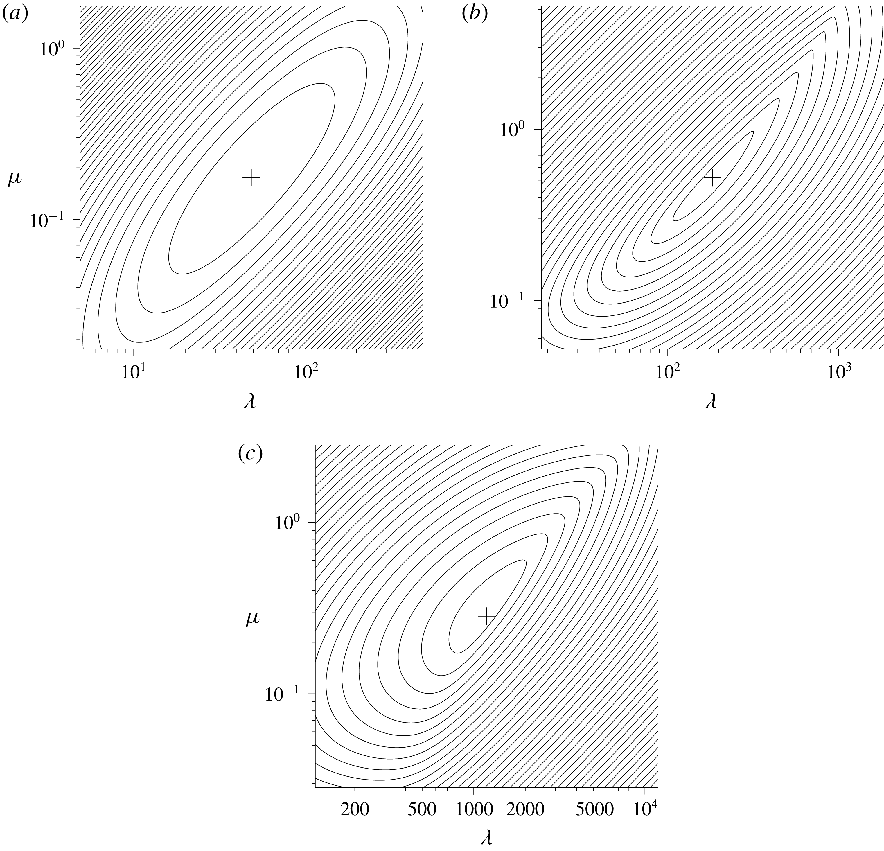
The evolution of
 $E(t)$
for the instability corresponding to the global maximum on the top curve of figure 10 is shown in figure 12(a) for stress-free boundary conditions. As the minimum is smooth, the condition for the ratios of
 $E_{K}(t)$
,
 $E_{T}(t)$
and
 $E_{M}(t)$
to be the same at
 $t=t_{0}=0$
and at
 $t=t_{1}=220$
are met. If one looks at the growth of
 $E(t)$
and its components in figure 12(a) this is confirmed. However the minimum of the growth of
 $E(t_{1})$
in figure 11(b), the instability with
 $\unicode[STIX]{x1D6FC}=0.141$
, is no longer smooth. The repeated eigenvalue gives rise to two independent modes being found by the numerics. Linear combinations of these two modes will also be optimal solutions. An example of the growth for one of these modes is shown in figure 12(b). The ratios of
 $E_{K}(t)$
,
 $E_{T}(t)$
and
 $E_{M}(t)$
evaluated at
 $t_{0}=0$
and at
 $t_{1}=220$
are different, confirming the minimum is not smooth.
Graph of the growth of
 $E(t)$
(solid lines) as functions of
 $t$
for
 $t_{0}=0$
and
 $t_{1}=220$
for (a) the optimum value of
 $\unicode[STIX]{x1D6FC}=0.126$
and (b) a representative example of
 $\unicode[STIX]{x1D6FC}=0.141$
, between two ‘bubbles’. The dashed lines show the corresponding contributions from (i)
 $E_{K}(t)$
, (ii)
 $\unicode[STIX]{x1D706}E_{T}(t)$
and (iii)
 $\unicode[STIX]{x1D707}E_{M}(t)$
.

The growth of both the instabilities in figure 12 show an initial adjustment for
 $t\lesssim 15$
, followed by an interval where there is relatively smooth growth up to around
 $t=80$
and
 $t=70$
respectively. At these points there are transitions where there is a dip in
 $E_{K}(t)$
, indicating the speed of the convection has almost come to a halt. Note that
 $E_{K}(t)$
does not drop to zero as it does for convection in a layer as the fluid does not come to a total rest everywhere at the same time in this reversal. After this reversal the instabilities follow the pattern of the growing diffusive instabilities in a layer. This shows that there are transitions between the initial states where the growths of the convection are relatively steady, as one would expect from temperature dominated convection, and the later state where the instabilities clearly have an oscillatory component to their growth as one would expect in double-diffusive convection in this diffusive regime. This transition is not unexpected from the trajectories of the instantaneous Rayleigh numbers shown in figure 9(a) where initially the thermal Rayleigh number is much greater than the salt Rayleigh number, and so one could expect that the salinity would be relatively unimportant and the convection essentially thermal (and non-oscillatory). Later on the salinity gradient comes into play, and the oscillatory diffusive convection predominates.
In figure 10, if the growth curves for intermediate values of
 $t_{1}$
were to be plotted, we would find that the left-hand bulges in the top two curves correspond to the second bulges in the corresponding curves immediately below. That is to say, as
 $t_{1}$
increases these bubbles in
 $E(t_{1})$
migrate to the left. As
 $t_{1}$
changes, so the wavenumber for the global maximum changes and, as one bulge takes over from another as the location of the global maximum, we will occasionally see a jump in value of the optimal wavenumber. The plot of the optimized growth,
 $E(t_{1})$
, as
 $t_{1}$
varies is shown in figure 13(a). The dashed and solid lines represent the local and global maxima of these curves respectively. Here we see the effect of these migrating bubbles. Each has a local maximum that is initially less than the global maximum, shown by the initial dashed portion of each curve. As
 $t_{1}$
increases the height of this maximum grows relative to the other maxima, until it has a period where it is the global maximum (shown by the solid portions of the lines). It then subsequently declines in relation to the others, shown by the final dashed portion of each of the lines, and ceases to be a local maximum when this line terminates. The corresponding wavenumbers,
 $\unicode[STIX]{x1D6FC}$
, for these maxima are shown in figure 13(b), where again the portions corresponding to the global maxima are shown as solid lines, and the other local maxima by dashed lines. The number of transitions of the fastest growing mode corresponds to the number of flow reversals observed in the instabilities. For example, there are three transitions before one reaches
 $t=220$
in figure 13(a), and there are three dips in
 $E_{K}(t)$
in figure 12(a) corresponding to points where there are reversals in the flow. There are more reversals for larger values of the wavenumber,
 $\unicode[STIX]{x1D6FC}$
, indicating a higher frequency of oscillations.
Plots of (a)
 $E(t_{1})$
and (b) the corresponding values of
 $\unicode[STIX]{x1D6FC}$
as a function of
 $t_{1}$
for the local maximum (dashed lines) and global maximum (solid lines) values of the optimized grows of
 $E(t_{1})$
for a stress-free bottom boundary.

The initial fragment of the curve clearly seen in figure 13(b) that does not fit in with the general trends corresponds to an initial instability that is essentially a thermal instability. This is consistent with the small-time results of KG. The instantaneous salt Rayleigh number is much smaller than the instantaneous thermal Rayleigh number, and so the initial development of the instability is essentially thermal. However, with the much smaller salt diffusivity even in this case the salt perturbation can grow significantly with time, and come into play. For much of the time range shown here the instabilities are clearly double diffusive in their nature, with the salinity playing a crucial role.
In figure 14 is shown a sequence of plots of the streamfunction and the temperature and salinity perturbations for the case with
 $t_{1}=220$
and
 $\unicode[STIX]{x1D6FC}=0.126$
. These have
 $t$
ranging from
 $t=135$
to
 $t=165$
, covering the middle reversal shown in figure 12(a). The contour spacing is based on the maximum perturbations up to that point in time. Hence, when the number of contours reduces it indicates that the corresponding perturbation is decreasing in magnitude. The top set of plots in the sequence shows a down-flow in the middle, with corresponding negative perturbations to the temperature and salinity. Because of the lower diffusivity of salt, this negative perturbation builds up, causing the flow to slow down and then reverse. At this point the negative temperature perturbation diffuses away and a positive perturbation is created by the up-flow. The up-flow reduces, and then reverses the salinity perturbation. This will then build up, and lead to the next reversal. Before the first reversal there is a longer period where the contours of the perturbations show little change, except for a small upwards growth at the top as the thermal layer grows in thickness.
Plots of the (a) streamlines, (b) contours of the temperature perturbation and (c) contours of the salinity perturbation for
 $t$
between 135 (top) and 165 (bottom) in steps of 5, for the case
 $t_{1}=220$
,
 $\unicode[STIX]{x1D6FC}=0.126$
and
 $Ra_{S}=1/40$
. The dashed lines show the contours with negative values.

The above results are for stress-free conditions at the bottom boundary. For the more realistic case with a no-slip boundary condition the optimized values of
 $E(t_{1})$
as a function of
 $\unicode[STIX]{x1D6FC}$
and for a selection of values of
 $t_{1}$
are shown in figure 15. This graph has the same vertical scale as shown in figure 10, emphasizing that the growth of these are notably lower than for the case of the stress-free boundary conditions seen before. The sequence for the no-slip case omits the curve for the first time shown in the previous plot,
 $t_{1}=40$
, and the last curve for
 $t_{1}=340$
is shown as a dotted line to differentiate it from the
 $t_{1}=280$
case. It can be seen that there is little growth between these last two times.
Graphs of the optimized
 $E(t_{1})$
as a function of
 $\unicode[STIX]{x1D6FC}$
for
 $t_{1}=100,160,220,280$
(solid lines, from bottom to top) and
 $t=340$
(dotted line) for no-slip boundary conditions with
 $t_{0}=0$
,
 $\unicode[STIX]{x1D70E}=7$
,
 $\unicode[STIX]{x1D70F}=1/80$
and
 $Ra_{S}=1/40$
. Also shown are the corresponding second eigenvalues (dashed lines).

If we look at the evolution of the maxima and their corresponding wavenumbers, shown in figure 16, we see that the behaviour is similar to the stress-free case. However, the overall growth is lower, and the overall growth towards the end of the time interval shown is coming to an end, and for larger values of
 $t_{1}$
the instabilities show a decline in the maximum growth.
Plots of (a)
 $E(t_{1})$
and (b) the corresponding values of
 $\unicode[STIX]{x1D6FC}$
as a function of
 $t_{1}$
for the local maximum (dashed lines) and global maximum (solid lines) values of the optimized growth of
 $E(t_{1})$
for a no-slip bottom boundary.

In the stress-free and no-slip cases shown in this section, the initial onset of instability is essentially convective for the sudden increase in the bottom boundary temperature. The optimized instabilities essentially grow from the start, and so the effect of varying
 $t_{0}$
was at best minimal. This was the case of heating a body of fluid from below with a sudden increase in temperature without a salinity gradient as investigated in KG. Hence, the variation of
 $t_{0}$
has not been considered explicitly in this section.
4.2 Constant heat flux
In this subsection we will look at the case of a constant heat flux at the bottom boundary. This is the case looked at previously, both experimentally and numerically, by Turner & Stommel (Reference Turner and Stommel1964), Huppert & Linden (Reference Huppert and Linden1979), Fernando (Reference Fernando1987), Kerpel et al. (Reference Kerpel, Tanny and Tsinober1991), Kazmierczak & Poulikakos (Reference Kazmierczak and Poulikakos1990) and Molemaker & Dijkstra (Reference Molemaker and Dijkstra1997). However, they did not investigate in any detail the actual onset of the convection. For the case of a constant heat flux at the boundary there is a vertical temperature gradient
 $\overline{T}_{z}(0,t)=-C$
at the wall (with
 $C>0$
). We use the length-scale
 $L$
in the non-dimensionalization such that
 $$\begin{eqnarray}\displaystyle \frac{g\unicode[STIX]{x1D6FC}CL^{4}}{\unicode[STIX]{x1D708}\unicode[STIX]{x1D705}_{T}}=1. & & \displaystyle\end{eqnarray}$$
We will use the scalings for the temperature and the salinity
 $$\begin{eqnarray}\displaystyle \unicode[STIX]{x0394}T=-\overline{T}_{z}(0,t)L=CL,\quad \unicode[STIX]{x0394}S=-\overline{S}_{z}L. & & \displaystyle\end{eqnarray}$$
This gives the governing equations for the perturbations:
 $$\begin{eqnarray}\displaystyle & \displaystyle \frac{1}{\unicode[STIX]{x1D70E}}\frac{\unicode[STIX]{x2202}\unicode[STIX]{x1D714}}{\unicode[STIX]{x2202}t}=-\frac{\unicode[STIX]{x2202}T}{\unicode[STIX]{x2202}x}+R_{\unicode[STIX]{x1D70C}}^{-1}\frac{\unicode[STIX]{x2202}S}{\unicode[STIX]{x2202}x}+\unicode[STIX]{x1D6FB}^{2}\unicode[STIX]{x1D714}, & \displaystyle\end{eqnarray}$$
 $$\begin{eqnarray}\displaystyle & \displaystyle \unicode[STIX]{x1D6FB}^{\prime 2}\unicode[STIX]{x1D713}=-\unicode[STIX]{x1D714}, & \displaystyle\end{eqnarray}$$
 $$\begin{eqnarray}\displaystyle & \displaystyle \frac{\unicode[STIX]{x2202}T}{\unicode[STIX]{x2202}t}-\text{erfc}\left(\frac{z}{2t^{1/2}}\right)\frac{\unicode[STIX]{x2202}\unicode[STIX]{x1D713}}{\unicode[STIX]{x2202}x}=\unicode[STIX]{x1D6FB}^{2}T, & \displaystyle\end{eqnarray}$$
 $$\begin{eqnarray}\displaystyle & \displaystyle \frac{\unicode[STIX]{x2202}S}{\unicode[STIX]{x2202}t}-\frac{\unicode[STIX]{x2202}\unicode[STIX]{x1D713}}{\unicode[STIX]{x2202}x}=\unicode[STIX]{x1D70F}\unicode[STIX]{x1D6FB}^{2}S, & \displaystyle\end{eqnarray}$$
 $R_{\unicode[STIX]{x1D70C}}$
, is given by
 $$\begin{eqnarray}\displaystyle R_{\unicode[STIX]{x1D70C}}=\frac{\unicode[STIX]{x1D6FC}(-C)}{\unicode[STIX]{x1D6FD}(\overline{S}_{z})}. & & \displaystyle\end{eqnarray}$$
When this parameter is used in the context of oceans, the requirement for a stable density gradient gives rise to the restriction that
 $R_{\unicode[STIX]{x1D70C}}<1$
for the diffusive regime (see, for example, Radko Reference Radko2013). However, this restriction does not apply here as the density gradient adjacent to the wall may have an unstable density gradient. In this subsection we will focus on the case with a no-slip boundary condition.
For the case of a fixed rise in the temperature at the wall it was found that, just as for the case of heating a body of fluid from below in KG, the effect of varying
 $t_{0}$
was not significant in enhancing the growth for a given
 $t_{1}$
. However for the case of a constant heat flux there is a more pronounced effect. This is shown in figure 17. In (a) the optimized growth is shown as a function of
 $\unicode[STIX]{x1D6FC}$
when
 $t_{1}=160$
for the case
 $t_{0}=0$
and
 $R_{\unicode[STIX]{x1D70C}}=1.8$
. The maximum size of the instability barely exceeds that of the initial state. If one looks at the evolution of this instability for
 $\unicode[STIX]{x1D6FC}=0.27$
, as shown in (b), it is clear that the instability actually undergoes a significant decay before recovering its amplitude. In (c) and (d) are shown the corresponding figures but with
 $t_{0}=60$
. Now there is substantial growth over the range of values of
 $\unicode[STIX]{x1D6FC}$
, and there is clear growth, with some degree of modulation, from around
 $t=80$
onward. This modulation corresponds to half oscillations in the growing instability. There is a growth in
 $E(t)$
of around 10 between each modulation at the later stages of this growth. The dependency of
 $E(t_{1})$
on
 $t_{0}$
for this value of
 $\unicode[STIX]{x1D6FC}$
is shown in figure 18(a). It should be noted that although this curve shows a maximum in
 $E(t)$
, this does not mean that the growth for larger values of
 $t_{0}$
has slowed down in any way. The decrease is mainly a reflection of the reduced time,
 $t_{1}-t_{0}$
, for the growth to take place. The effective rate of growth of
 $E(t)$
increases as
 $t$
increases as shown in figure 18(b) where the effective growth rate of the instability between
 $t_{0}$
and
 $t_{1}$
is given by
 $$\begin{eqnarray}\displaystyle p_{eff}=\frac{\log (E(t_{1})/E(t_{0}))}{2(t_{1}-t_{0})}. & & \displaystyle\end{eqnarray}$$
Here it can be seen that the effective growth rate is essentially increasing, showing that the evolving heated layer is becoming more unstable as time increases, unlike the previous case with the sudden increase in the wall temperature where the heated layer becomes less unstable, and eventually stable, as the temperature profile evolves.
Graphs with
 $t_{0}=0$
and
 $t_{1}=160$
for
 $R_{\unicode[STIX]{x1D70C}}=1.8$
and
 $\unicode[STIX]{x1D6FC}=0.27$
of (a)
 $E(t_{1})$
as a function of
 $\unicode[STIX]{x1D6FC}$
and (b) the corresponding growth of the mode. The corresponding graphs with
 $t_{0}=60$
are shown in (c) and (d).

Graph of (a)
 $E(t_{1})$
and (b)
 $p_{eff}$
, the effective growth rate, as
 $t_{0}$
is varied for a constant heat flux. Here
 $R_{\unicode[STIX]{x1D70C}}=1.8$
,
 $t_{1}=160$
and
 $\unicode[STIX]{x1D6FC}=0.27$
.

Contour plots of
 $E(160)$
as a function of
 $t_{0}$
and
 $\unicode[STIX]{x1D6FC}$
. The contour levels for the heavy lines are
 $E(160)=1,10,10^{2},10^{3},\ldots ,$
with the lighter lines evenly spaced in between.

A contour plot of the growth in
 $E(t_{1})$
for the case of
 $t_{1}=160$
for a range of
 $\unicode[STIX]{x1D6FC}$
and
 $t_{0}$
is shown in figure 19. This shows a relatively smooth maximum, but with superimposed ridges from the bubbles associated with each oscillation. This leads to there being several local maxima, with the global maximum located near
 $\unicode[STIX]{x1D6FC}=0.3010$
and
 $t_{0}=69.58$
. As with the sudden increase in temperature case, the larger number of ridges to the right indicate a higher frequency of oscillations for larger wavenumbers.
Lastly we will look at the fully optimized solutions, including varying
 $t_{0}$
, for a range of
 $R_{\unicode[STIX]{x1D70C}}$
. We will look at the case
 $t_{1}=240$
which shows the salient features. The maximal growth of the instabilities is shown in figure 20(a) as a function of
 $R_{\unicode[STIX]{x1D70C}}$
, with the corresponding values of
 $t_{0}$
,
 $\unicode[STIX]{x1D6FC}$
and
 $p_{eff}$
shown in figure 20(b–d). As can be anticipated from the contours of the growth in figure 19, for each
 $R_{\unicode[STIX]{x1D70C}}$
there are multiple local maxima to the optimized
 $E(t_{1})$
as a function of
 $\unicode[STIX]{x1D6FC}$
and
 $t_{0}$
, some of which are very close in height. For the larger values of
 $R_{\unicode[STIX]{x1D70C}}$
shown here the peak that corresponds to the global maximum changes relatively slowly as
 $R_{\unicode[STIX]{x1D70C}}$
varies, and so we can plot curves corresponding to the respective values at the global maximum. For the lower values of
 $R_{\unicode[STIX]{x1D70C}}$
there is a relatively rapid change, and we plot the values found as points as they often correspond to different ridges. The plot of
 $E(t_{1})$
is, however, plotted as a continuous curve as the range of values for the top local maxima found is relatively small, and on this logarithmic plot would be indistinguishable. The small discontinuities in its gradient where the location of the global maximum shifts between the local maxima, in a similar way to the curve of the optimum
 $E(t_{1})$
seen previously in figure 13, would not be visible here.
Graphs of (a)
 $E(t_{1})$
, (b)
 $t_{0}$
, (c)
 $\unicode[STIX]{x1D6FC}$
, (d)
 $p_{eff}$
and (e) instantaneous
 $Ra_{T}$
(upper line) and
 $Ra_{S}$
(lower line) at
 $t=t_{0}$
for the fully optimized solution with
 $t_{1}=240$
, with
 $\unicode[STIX]{x1D70E}=7$
and
 $\unicode[STIX]{x1D70F}=1/80$
.

In figure 20(a) it can be seen that there is a dramatic variation in the growth of the instabilities,
 $E(t_{1})$
, as
 $R_{\unicode[STIX]{x1D70C}}$
varies. There is a low value of around
 $16$
when
 $R_{\unicode[STIX]{x1D70C}}=1.4$
to an un-physical high value of over
 $10^{31}$
when
 $R_{\unicode[STIX]{x1D70C}}=2.0$
. In real situations, the growth that is required for instabilities to be observed and for nonlinear effects to come into play is not clear. However, it is probable that
 $16$
is too low, and
 $10^{31}$
is far more than is required. There are two main effects that combine to create this large variation in
 $E(t_{1})$
. Firstly the time available for instabilities to grow increases as
 $R_{\unicode[STIX]{x1D70C}}$
increases, as shown by the variation of
 $t_{0}$
in figure 20(b). Secondly the effective growth rate of the disturbances, shown in figure 20(d), also increases by a factor of around
 $5$
in this range of
 $R_{\unicode[STIX]{x1D70C}}$
.
The instantaneous Rayleigh numbers
 $Ra_{T}$
and
 $Ra_{S}$
evaluated at the time,
 $t_{0}$
, of the onset of the instabilities are shown in figure 20(e). In terms of the non-dimensional unit used here, the instantaneous values of
 $Ra_{T}$
and
 $Ra_{S}$
, based on the instantaneous length scale,
 $(\unicode[STIX]{x1D705}_{T}t)^{1/2}$
, and the instantaneous wall temperature and the vertical salinity gradients are
 $$\begin{eqnarray}\displaystyle Ra_{T}=\frac{2t^{2}}{\unicode[STIX]{x03C0}^{1/2}},\quad Ra_{S}=R_{\unicode[STIX]{x1D70C}}^{-1}t^{2}. & & \displaystyle\end{eqnarray}$$
The value of these at the time of onset of instability reflect the significant delay in the onset of the growth of the instabilities,
 $t_{0}$
. Particularly for the lower values of
 $R_{\unicode[STIX]{x1D70C}}$
shown here, these are comparable to the values that may be expected from the naive comparison with the critical Rayleigh numbers shown in figure 9(b) for a layer. This is unlike the case of the sudden increase in the boundary temperature seen in the previous subsection (and in KG). At the initial stages for the step increase in temperature the instantaneous values of
 $Ra_{T}$
grow faster than
 $Ra_{S}$
and the initial instabilities are close to the thermal case. In that case comparing the instantaneous Rayleigh number to the classical problem of convection in a layer would be misleading. With a constant heat flux the instantaneous Rayleigh numbers grow in tandem, and the disturbances seem to be intrinsically double diffusive for their entire evolution, as can be seen by the wriggly growth curve shown in figure 17(d), and so there seems to be an intrinsic difference between the cases of sudden heating and constant heat flux.
5 Conclusion
In this paper we have two main thrusts. The first was to extend the method of Kerr & Gumm (Reference Kerr and Gumm2017) that was used for time-dependent thermal convection to time-dependent double-diffusive convection in order to give a framework for the analysis of these problems. The second thrust was to apply this method to the basic problem of the sudden heating from a horizontal boundary of a fluid with a stable salinity gradient.
An important aspect of the method of KG was to identify an appropriate measure of the amplitude of the disturbances. The measure of the amplitude that was identified here as being effective for the double-diffusive case was
 $$\begin{eqnarray}\displaystyle E(t)=\frac{1}{2P}\int _{0}^{\infty }\int _{0}^{P}|\boldsymbol{u}|^{2}+\unicode[STIX]{x1D706}T^{2}+\unicode[STIX]{x1D707}(S-\unicode[STIX]{x1D6FE}T)^{2}\,\text{d}x\,\text{d}z. & & \displaystyle\end{eqnarray}$$
The inclusion of the
 $\unicode[STIX]{x1D6FE}T$
term allows a more general quadratic measure for effect of heat and salt, and ensure that this is positive for positive
 $\unicode[STIX]{x1D706}$
and
 $\unicode[STIX]{x1D707}$
. The use of such a general quadratic term has been used previously in the energy stability analysis of Kerr (Reference Kerr1990). This measure works well with the adaption of the optimization method of KG for finding the maximum growth for given values of
 $\unicode[STIX]{x1D706}$
,
 $\unicode[STIX]{x1D707}$
and
 $\unicode[STIX]{x1D6FE}$
. These parameters were then adjusted to minimize this maximal growth. When considering double-diffusive instabilities in a layer, and the growth in
 $E(t)$
over a time interval was minimized by varying these parameters, the exponentially growing modes in the salt-finger regime were recovered. The solutions found in the diffusive regime were only a small perturbation away from the oscillatory modes found by Baines & Gill (Reference Baines and Gill1969). By choosing the parameters
 $\unicode[STIX]{x1D706}$
,
 $\unicode[STIX]{x1D707}$
and
 $\unicode[STIX]{x1D6FE}$
in this way, we have tried to adopt a general principal that avoids making an arbitrary choice of the measure of the amplitude, or the form of the initial conditions. This choice of measure of the amplitude minimizes artefacts in the evolution of instabilities in the layer that other options may present. If other methods were to be applied to more general problems such as the heating of a salinity gradient, these artefacts cannot be expected to go away. Hence using
 $E(t)$
, and choosing
 $\unicode[STIX]{x1D706}$
,
 $\unicode[STIX]{x1D707}$
and
 $\unicode[STIX]{x1D6FE}$
to minimize its growth, was the best approach that we found. Whether there are other approaches that are, in some sense, ‘better’ is hard to say – but we have not found them.
When investigating the behaviour of salt-stratified body of fluid heated from a horizontal bottom boundary we considered two cases: a sudden increase in bottom temperature and the sudden starting of a constant heat flux. These two cases are clearly related, but with some significant differences.
For the purely thermal case of heating a body of fluid from below, looked at by KG, it was found that instabilities formed almost instantaneously. Hence taking
 $t_{0}=0$
gave growth that was optimal, or nearly optimal. This is also the case here for the case of a constant temperature increase at the boundary. This may be anticipated as during the initial stages the effective instantaneous salt Rayleigh number is much smaller than the corresponding instantaneous temperature Rayleigh number, and thermal effects dominate with the instabilities having an initial non-oscillatory phase. Given the double-diffusive instability is essentially thermal at the onset of heating, with the salinity gradient not important, taking
 $t_{0}=0$
gives optimal, or near optimal, growth too. However, for the constant heat-flux case the ratios of the effective instantaneous temperature and salt Rayleigh numbers are constant, and so the salinity gradient is important throughout and there is no initial thermal phase. In this constant heat-flux case disturbances initially decay, and to maximize the growth at some time,
 $t_{1}$
, a non-zero
 $t_{0}$
must be used.
The investigation of the constant heat-flux case focused on
 $R_{\unicode[STIX]{x1D70C}}$
in the range
 $1.4$
to
 $2$
as these spanned behaviours from slow growth to quite rapid growth when compared to the time scales of the oscillations. Although the density gradient at the wall is destabilizing for all these values of
 $R_{\unicode[STIX]{x1D70C}}$
, the instabilities observed are not just density driven. Their oscillatory evolution clearly indicates that it was diffusive instabilities that were observed from the onset of convection.
In the various experiments and numerical calculations conducted on this problem the values of
 $R_{\unicode[STIX]{x1D70C}}$
were significantly higher than the range considered here, for example Kazmierczak & Poulikakos (Reference Kazmierczak and Poulikakos1990) used
 $R_{\unicode[STIX]{x1D70C}}=3$
or
 $10$
. The focus on these investigations was on the development of a sequence of convecting layers, one above the other. The investigation of the nature of the onset of instability and its initial evolution were not particularly relevant to these investigations. With these larger values of
 $R_{\unicode[STIX]{x1D70C}}$
we would anticipate a rapid growth of the instabilities, which was observed. No direct comparison between the results here and the previous experimental and numerical investigations are possible.
It is hoped that this approach will also provide insight into double-diffusive instabilities observed when a salt-stratified body of fluid is heated at a side wall and other related problems such as instabilities at a sloping boundary to a fluid with vertical temperature and salinity gradients looked at by Linden & Weber (Reference Linden and Weber1977). Some such problems can be investigated using a quasi-static or frozen-time analysis, usually when there is relatively slow heating of the fluid (Kerr Reference Kerr2000), but there are many cases where such an analysis cannot be applied. Although there have been speculations to mechanism involved in these instabilities based on experimental observations, (see, for example, Schladow et al. Reference Schladow, Thomas and Koseff1992), a theoretical investigation that takes into account the time dependency of the background state has not been possible. It is hoped that applying the methods used here will address that deficiency, and may be compared to experimental observations where the onset of convection was often of interest. This is under investigation.



