


1. Introduction
Ice streams of the Antarctic and Greenland ice sheets account for a large fraction of total ice-sheet drainage (Morgan and others, 1982; Paterson, 1994, p. 301). Geologic and palacoceanographic evidence suggests that ice streams and fast-flow behaviour (e.g. surge lobes, Heinrich events) played an equally vigorous role in the history and dynamics of past ice sheets (e.g. Clark, 1991; Bond and Lotti, 1995). Despite this motivation, ice streams are not explicitly portrayed in large-scale ice-sheet models. The foremost limitation is the basic problem that fast-flow physics and ice-stream activation are not well understood. Scale imposes another fundamental restriction. Current ice-sheet models have grid-cell dimensions of order 20–100 km; contemporary ice streams are essentially sub-grid at this resolution.
We have developed a continuum mixture framework which overcomes the scale limitation. Ice-sheet area is divided into a binary mixture of sheet ice and stream ice. Conservation laws are applied to each component to track interdependent dynamic and thermal evolutions. This accounts for ice-stream fluxes without concomitant enhancements in resolution. The number of equations and field variables is doubled from conventional models, increasing computational cost by a factor of 2.
The mixture framework permits rational exploration of ice-stream physics. This paper focuses on parameterization of rules for sheet/stream coupling and controls of ice-stream activation and growth. We envisage two means by which ice is exchanged between flow regimes, creep transfer and bed transfer. Creep transfer describes ice-stream nourishment by viscous creep flow of ice from the ice sheet. Bed transfer can be thought of as a real activation or deactivation of ice streams and is controlled by basal conditions. We present ice-stream mobilization experiments on the EISMINT calibration block, a simplified ice geometry resting on a flat bed.
2. Theoretical Model
We outline the continuum foundation of the mixture model in this section, introducing a general formulation that can be applied to multiple ice-flow constituents. This paper considers a two-component mixture of sheet ice and stream ice, which honour distinct governing dynamics. Sheet ice flows by viscous creep deformation under gravitational loading, whereas stream-ice fluxes are driven by subglacial sediment deformation and/or decoupled sliding at the ice–bed contact. Because of this important distinction, we separately describe the velocity of each mixture constituent rather than blend the contributions to obtain a single barycentric velocity.
Consider an ice mass occupying total mixture volume V in a Cartesian reference frame (x 1, x 2, x 3). Directions x 1 and x 2 are horizontal and x 3 is vertical and positive upwards. Define mixture surface area S interior to V, with Euclidean area element dS = dx 1dx 2 and volume element dV = dx 3dS. An intensive quantity Ϋ(x 1, x 2, x 3, t) in volume V with vertical extent H has the integral value

where (Ϋ) is the vertical integral of Ϋ. Define the vertically averaged quantity

We employ summation convention for vector operations and tensor fields. As a general convention, subscripts i, k, and l denote three-dimensional operations and vectors, and we reserve subscript j for two-dimensional (horizontal operations and vectors. Define the three-dimensional velocity field v k(x 1, x 2, x 3, t) with components (u, v, w) and the horizontal sub-set v j(x 1, x 2, x 3, t) with components (u, v).
2.1. General balance equations
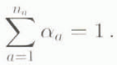
The nature of sheet/stream divisions in an ice mass leads us to describe a two-dimensional areal mixture rather than a volume mixture. We divide area S into na ice-flux constituents, where na = 2 in the binary sheet/stream mixture. Subscript a signifies constituent properties, with a ϵ (s, c) denoting sheet ice and stream (“channelized”) ice, respectively. The areal density or infinitesimal area fraction of each constituent is α a (x 1, x 2, t), with the saturation constraint
Constituents co-exist in S, each component occupying bed area α
a
S. Define constituent surface heights  and bed heights
 above an arbitrary datum (e.g. sea Level). Corresponding ice thicknesses are then

Note that constituents occupy distinct vertical space and there is no vertical variation in component fraction α a . For a general constituent thermodynamic quantity ϋ a in the areal mixture, this allows the simplification

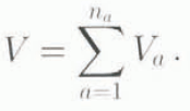
Total ice volume V is therefore composed of constituent volumes

with
Consider the time evolution of a specific constituent material quantity ϋ a , with the extensive integral value

We assume that ice is incompressible with a true mass density ρ that is constant and identical for all mixture ice components. The Lagrangian time derivative of Equation (8) gives the transport relation

where the spatial derivative  is over j ϵ (1,2) and d
a
/d
t
denotes the constituent material derivative. With Equation (1) the resulting expression (9) becomes

Now consider the kinematic conditions at the constituent surfaces (e.g. Hutter, 1983; Morland, 1984). Applying the constituent material derivative at the upper surface  .

where  is a source/sink term representing ice-equivalent supply rate (accumulation ablation) at the constituent surface. We define it to be positive for positive mass balance (net accumulation). Surface-ice velocities in the material derivative are defined in the horizontal plane which is approximated to be parallel to the surface. This is the common assumption made in ice-sheet models and requires small surface slopes with negligible deviations from the horizontal mean surface (Hutter, 1983). Similarly, at the constituent bed
 ,

where  incorporates basal melt and refreezing, and is again defined as positive for net gain of ice (refreezing exceeding melt). Leibnitz’ differentiation rule over the vertical integral gives

where r is a generalized time-space coordinate, r ϵ (x 1, x 2, t). Equations (11) – (13), along with Equation (5) simplify Equation (10) to give the vertically integrated Reynolds transport theorem

where we have combined terms  and
 into a single source/sink rate
 .
This is a general result for vertically integrated constituent balances. Define a specific transfer term X a which describes exchanges between mixture constituents in area S. This transfer term obeys
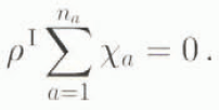
The balance law of a flux-free quantity  thus yields

Note that X a is the rate of supply of quantity ϋ a ; X a is vertically constant, emphasizing once again the areal basis of our mixture.
2.2. Mass balance
Consider now the particular case of mass balance, with ϋ a = 1 (dimensionless). Using Equation (6), constituent ice masses are given by

and the total ice mass is

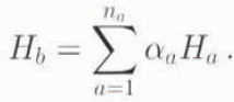
If one considers the ice volume as a whole with an average or bulk ice thickness Hb , the total ice mass can be written

With respect to Equation (18), this defines the bulk thickness
It is possible to model the full mixture evolution using this single variable and a corresponding barycentric velocity. This is appealing because it reduces the number of unknowns from 2na −1 to na but it sacrifices physical understanding. Component thicknesses and velocities have physical significance and different dynamics govern each flow component. We therefore choose to describe separate constituent evolutions, applying the transport theorem to each mixture component based on constituent velocities vak .
For a specific mass-exchange rate X ad with dimension LT −1 Equation (16) with ϋ a = 1 gives

From Equations (14) and (17), this gives the global balance

This has the local form

This is the governing equation for constituent ice-thickness evolution where the areal partitioning α
a
(x
1, x
2, t) is known. A separate evolution equation for α
a
(x
1, x
2, t) is required. We are working towards an evolution equation which determines α
a
from bed character and bed thermal and hydrological conditions (paper in preparation by S. J. Marshall and G. K. C. Clarke). For simplicity, here α
a
(x
1, x
2, t) is a prescribed function. Constitutive relations and momentum equations for each flow component are applied to express  in terms of constituent ice thickness, closing Equation (23). The specific form of Equation (23) for each constituent in the ice mixture is described below.
3. Application to the Sheet/Stream Mixture
3.1. Mass balance
We now apply the generalized vertically integrated dynamics to a binary ice-sheet/ice-stream mixture (Fig. 1), using subscripts to denote sheet ice and subscript c for stream ice. We consider each constituent to occupy the same bed, such that  for a ϵ (s, c). Local constituent thicknesses are then


and from Equation (17) the masses of sheet ice and stream ice are
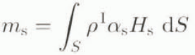

The total ice mass is

and the bulk thickness of ice in area S, from Equation (20), is

Define mass-balance rates ḃs(x 1, x 2, t) and ḃc(x 1, x 2, t) which represent net accumulation minus ablation for each constituent, including upper surface and basal contributions. Define the mixture exchange term X ad in Equation (23) as ρ md , positive for transfer from the sheet ice to the stream ice; explicitly,ρ sd = −ρ md and ρ cd = ρ md . Local constituent mass-balance equations then follow,

and the analogous stream component balance

Equation (28) bear close resemblance to the vertically-integrated conservation equation of Mahaffy (1976), weighted by the areal fraction in our case. Coupling/exchange terms ρ
md
and  are discussed below. Note that the saturation constraint (3) requires
 .
Plan view of the areal mixture of sheet ice, fraction ±s, and stream ice, fraction αc = 1 − αs depicts areal division over the full ice sheet, with area S, and (b) visualizes sample finite-difference cells containing ice streams with αc ≈ 0.3.

3.2. Ice-sheet and Ice-stream fluxes
We assume that sheet ice flows by viscous creep deformation following Glen’s flow law (Glen, 1958; Paterson, 1994. p. 97). Stream-ice fluxes are basally driven, with low basal shear stress and high velocities such that internal creep deformation is negligible. Glen’s flow law relates strain rates ⋵ ik to deviatoric stresses σʹ ik , in the ice

where Σʹ2 is the second invariant of the deviatoric stress tensor,
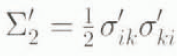
and B(T 1) is a strain hardness or viscosity term which follows the Arrhenius temperature dependence

Q is a creep activation energy, R gas is the ideal gas law constant. B 0 is a constant and n is the flow-law exponent, typically set to 3.
We assume vanishing interaction forces for constituent force balances. The ice-sheet mass balance (Equation (28a)) can then be closed using Mahaffy’s (1976) reduced system of momentum equations winch express viscous creep flux as a function of ice thickness and topography. In the ease where sheet ice is treated as isothermal at mean temperature  . Glen’s flow law and the vertically integrated momentum equations give the horizontal velocity components u
s(x
3) and v
s(x
3):

The notation  indicates the L
2 norm of vector
 . Integrating again over the ice thickness gives the ice fluxes

Equations (28a) and (33) give a non-linear parabolic equation which tracks ice-sheet thickness and velocity-field evolution.
We model ice-stream fluxes in Equation (28b) as basally driven with no internal shear, giving plug flow with

For the sensitivity tests described in this presentation, we specify basal velocities rather than calculate them from a momentum-balance equation. We are working towards a more complete physical treatment to parameterize objectively vcj (h B) as a function of basal-water pressure, areal coverage of water at the bed and basal and marginal pinning points (basal and side drag).
Exchanges of momentum between flow constituents may be quite important as a velocity control on ice streams. A sensible way to introduce ice-stream mechanics and sheet/stream coupling would be to apply the reduced ice-shelf dynamical equations (Morland, 1987). MacAyeal (1989) and Jenson (1994) have previously adapted these equations to descriptions of ice-stream and surge-lobe flow. Parameterizations for basal drag are required and similar parameterizations could be made to describe side drag exerted by the sheet ice.
3.3. Dynamic coupling
The source/sink term X md , in Equations (28 represents transfer of ice between ice-sheet and ice-stream components. We describe two means by which the domains exchange ice mass; creep capture X b , governed by ice dynamics and bed capture X b , governed by bed properties and basal hydrological and thermal conditions.
Creep capture is one-way; it is the creep flow of ice from the ice sheet to the ice stream. This is specified from the Glen flow parameters B and n, ice-sheet thickness H
s
and the gradient in height  across a characteristic horizontal length stale L, hence

We have introduced a dimensionless constant X 0 which controls the strength of creep capture. It may embody cell characteristics such as the ice-stream path length (exchange-zone length) and is of order 1. We choose length scale L to be the horizontal dimension of the finite-difference cell.
Bed capture X
b
, is the interchange of ice mass due to conversion of bed area from one flow regime to the other, following  . To convert this to ice mass (volume) exchange in Equation (28), the area of the bed being transferred must be multiplied by the height of the corresponding ice column. This depends on the direction of the conversion. We introduce a generalized representation

This notation is adapted from a similar Boolean operator used by Patankar (1980).
The full source/sink term in Equation (28) is X
md
= X
x
+ X
b
. The latter acts as the effective control of ice-stream mobilization, while X
x
is the dominant exchange term which feeds fully developed ice streams. There may appear to be double accounting of the areal exchange term, as a  term arose naturally from the mass balance in Equation (28). Depending on the sign, this original term and X
b
combine to either cancel out or give a disbalance
 . This is sensible; if ice-sheet and ice-stream thicknesses are identical, thickness fields are not perturbed by transferring bed area.
3.4. Vertical velocity-field computation
The vertical velocity field in each constituent is found from the distribution of horizontal velocities ua (x 1, x 2, x 3, t) and v a (x 1, x 2, x 3, t) and from the mass-balance Equation (21) for incompressible ice

In this instance, we consider the three-dimensional balance and write the vertically constant exchange term as a volume integral

The local form of the global constituent balance is

This can be expanded to give an integral expression for the constituent vertical velocity field

Constituent-exchange term X ad is given by X x + X b , from Equations (35) and (36), with X sd = −X md and X cd = X md , giving

This gives the full three-dimensional flow field which is of interest in particle tracking and in thermal advection for thermomechanical modelling.
3.5. Initial and boundary conditions
The coupled sheet stream dynamical evolution is governed by Equations (28a and b), which contain the unknowns  and X
md
. Constituent ice-surface topographies
 and
 are our two unknowns which are freely determined from arbitrary initial values. Bed topography h
B is a specified initial field and is fixed (no isostatic adjustment) in tests presented here. Ice-sheet velocity
 , is calculated from ice and bed topographies using Equation (33). Scenarios are prescribed for ice-stream velocity
 , for areal partitioning α
s
(x
1, x
2, t) and for mass-balance rates ḃ
s
(x
1, x
2, t) and ḃ
c
(x
1, x
2, t). Initial area] partitioning is arbitrary; we begin with pure sheet ice (α
s
= 1) everywhere. The exchange term X
md
is calculated from Equations (35) and (36), and is a function of
 , α
s
and
 .
Constituent ice thickness is forced to zero at lateral boundaries by specifying instantaneous ablation of all ice which reaches the margins. In a steady state, net mass loss at the boundaries should equal net gain From ḃ s , and ḃ c .
4. Numerical Model
Ice dynamics are solved in a three-dimensional finite-difference model styled after Huybrechts (1990, 1992). Models in this class are based in principle on the dynamic treatment of Mahaffy (1976). Our model has been developed in a spherical Cartesian coordinate system but it readily emulates a rectangular coordinate system for the tests presented here. Consider (x 1, x 2, x 3) to map to (x, y, z); the finite-difference model has extent (n x , n y , n z ) and the corresponding cell dimensions (△ x , △ y , △ z ).
The sheet/stream mixture doubles the number of field variables at each finite-difference cell and also introduces the new variable α
s
(x
1, x
2, t) which describes areal fractionation. This requires a further step in the numerical procedure. Areal divisions are determined within each finite-difference cell prior to the dynamic update to give the required variables α
s
and  . We then employ an Alternating Direction Implicit (ADI) scheme to update ice-surface evolution (Equation (28)), after Mahaffy (1976). Sheet and stream surfaces are jointly solved in a matrix system now doubled in size. Because the sheet-ice equation is extremely non-linear. Newton’s method is applied at each time step to iterate to an acceptable convergence criteria (r.m.s. residual of less than 10−6 m a−1 in each ADI sweep n
x
or n
y
cells).
The physical determination of α
s
is governed by basal processes which are in turn controlled by a collaboration of ice dynamics, basal thermal and hydrological regimes, and bed geologic and topographic coupling with the ice. A respectable physical treatment of the problem requires description of this full range of system controls. We limit this paper to simple tests of the mixture framework and hence prescribe scenarios for the areal division, as detailed below. A full thermomechanical mixture model has been developed and coded (paper in preparation by S. J. Marshall and G. K. C. Clarke) and we are now in the process of developing a hydrological model that responds to basal thermal and mechanical conditions. Primary controls of dynamic areal partitioning α
s
(x
1, x
2, t) are sub-grid distribution and pressure of water. In addition, we envisage a limiting  in each cell determined by sub-grid topographic and geologic attributes. This is the maximum cell area which could support ice streams, essentially a bed predisposition.
5. Sensitivity Tests
We explore exchange rules and coupled behaviour on the EISMINT intercomparison ice block. This ice block is simple enough to permit controlled and economic sensitivity analyses. The EISMINT test domain was set up by Huybrechts and others (1996) at EISMINT Model Intercomparison Workshops in Brussels (June, 1993) and Bremerhaven (June. 1994). Huybrechts and others (1996) provided a comprehensive discussion of model specifications and workshop results. We summarize base-model characteristics here and describe mixture-model behaviour for ice streams introduced along the EISMINT transect.
5.1. Base model characteristics
Model domain is a 1500 km ×1500 km block with 50 km grid cells, giving a horizontal extent n x = n y = 30. We applied a 15 level vertical resolution in all results presented here. The control-case ice-sheet bed is flat and at sea level (h B = 0), and there is no bedrock adjustment to ice-sheet loading in these tests. Initial ice thickness is zero and a spatially uniform accumulation rate of 0.3 ma−1 is applied for all time. All ice which reaches the margins ablates instantaneously. Table 1 summarizes physical and model parameters used throughout. Under pure creep flow, the ice sheet takes 40–100 ka to reach equilibrium (varying with model intricacy).
Physical and model parameters

Equilibrium fields for pure sheet, flow in the EISMINT model test block, (a) Plan view of ice-thickness contours for thermally decoupled flow, (b) Profiles of ice thickness and average column velocity, ü, along the EISMINT transect shown in (a).

Equilibrium dynamic profiles from an experiment with an ice stream from x = 1100–1500 km along the EISMINT transect. All profiles are at 20 ka, with αc, = 0.5 and X 0 = 1 (a) shows thickness contours, (b) Graphs of transect surface profiles, where the upper curve is the initial thickness, (c) shows depth-averaged ice-sheet and ice-stream velocities and (d) shows time series of divide thickness, transect volume and ice-stream head thickness.

Thinning of (a) sheet and (b) stream ice along the EISMINT transect as a function of creep-coupling strength X x. From top to bottom, curves correspond to X 0 = (0.01, 0.1, 0.5, 1, 5, 10). The ice-stream head is 350 km from the divide.

We use equilibrium isothermal ice sheets as initial/base models for the sensitivity tests. Ice is set to 273 K, giving a flow-law coefficient  which corresponds to the EISMINT level 1 tests Huybrechts and others, 1996). Figure 2 presents base-model equilibrium thickness and velocity fields. Transect profiles are plotted for y = 750 km along x = 750–1500 km.
5.2. Ice-stream profiles
We introduce a single ice stream along the EISMINT transect, beginning 350 km from the ice divide and extending 400 km to the margin. It is limited to one grid cell in width (50 km). An ice-stream outlet velocity uc
= 900 m a−1 is imposed, decreasing linearly to zero at the head of the stream. Velocities are fixed at this level for as long as the stream is active. The ice stream is activated and grown by areal transfer of sheet ice within the transect cells. The initial configuration (time 0) contains pure sheet ice (α
c
= 0) throughout. Ice-stream bed fractions along the transect are then ramped up to 50% (α
c
= 0.5) over 500 years, at a constant rate  . Areal partitioning is held at this level for the duration of the experiment, 10–20 ka. This corresponds to an ice stream nominally 25 km in width, although this is not explicit in the mixture. Creep exchange is active throughout, with an exchange coefficient X
0 = 1 in this initial activation test.
Figure 3 shows thickness and velocity profiles and time series from a typical activation experiment. The ice stream immediately initiates a surface lowering along its axis and in adjacent cells, as ice flux out of the system increases. Following a transient period of about 3 ka, a new equilibrium is reached; ice thicknesses and total volume are constant for the rest of the integration. The upper curve in figure 3b is the initial base-model thickness profile and the lower curves show sheet- and stream-ice profiles along the EISMINT transect after 20 ka. There is a surface draw-down of about 100 m at the divide and over 400 m midway along the stream. Plot figure 3c displays depth-averaged horizontal ice velocities ū s and ū c along the transect. Creep velocities are dramatically reduced due to surface lowering and flattening, consistent with expectations under thin and low-sloping ice. Ice-stream surface draw-down and upwards concavity are observed in Antarctic ice streams, particularly near their head (Shabtaie and others, 1988). Plot figure 3d depicts the time evolution of ice-divide and ice-stream head thicknesses and total transect-ice volume.
Time series of ice-divide thickness, transect-ice volume and ice-sheet thickness at the ice-stream head, (a) corresponds to X 0 = 0.1 and (b) displays oscillations enticed by greater creep coupling, X 0 = 5.

Equilibrium dynamic profiles from an experiment with five-fold increases in ice-stream velocity. All profiles are at 10 ka, with X c = 0.5 and X 0 = 0.1. (a) plots thickness contours, (b) plots transect profiles and (c) displays depth-averaged velocities as in Figure 3. (d) shows time series of divide thickness, transect volume and sheet thickness at the ice-stream head. Note the greatly enhanced thinning relative to Figure 3.

5.3. Creep capture of ice
We varied creep-capture coefficient X 0 in a set of experiments with the single-stream model. Stream activation, velocity and positioning were prescribed in section 5.2. The creep-coupling parameterization (Equation (35)), has its physical basis in reasonably constrained quantities, from ice properties and Glen’s flow law. We therefore anticipate that the coefficient ͼ n ≈ 1. A range of simulations varying ͼ0 from 0.01 to 10 affirms this, with unphysical or high-strung behaviour exhibited beyond this range. In all cases, ice-thickness and velocity profiles are identical in form to those in Figure 3. Ice-stream profiles are concave-upwards except at the outlet, where zero thickness is enforced in these tests: given free reign, stream flow across the boundary gives an ice cliff which more closely resembles a calving front.
Figure 4 plots sheet and stream thinning along the transect, relative to the initial (base-model) thickness. All profiles are at 20 ka and are equilibrated. The head of the ice stream is 350 km from the divide and stream thicknesses plotted above this simple track-sheet thickness (α
x
, = 0 at these points). The impact of X
0 on sheet-ice elevations is almost indiscernible. Stream-ice evolution is more sensitive to creep-exchange strength, with thinner ice streams under low coupling. As X
0 increases, sheet and stream thicknesses track each other more closely and the resulting ice stream thickens. There is essentially a balance between X
0 and  which adjusts
 to meet the feeding requirements of the ice stream.
Behaviour at the ice-stream head becomes interestingly sporadic when X 0 increases, as seen in time series plotted in Figure 5). The pint in figure 5a corresponds to the case X 0 = 0.1 and figure 5b is for X 0 = 5. The former case smoothly approaches and maintains equilibrium thicknesses, velocities and transect volume. Sheet flow at the head of the ice stream has more than doubled from the initial configuration as a result of surface steepening. This is important for ice-stream nourishment from the peripheral sheet ice. Under enhanced creep coupling in the lower plots, the ice-stream head appears unstable. Ice at the divide and elsewhere quickly approaches equilibrium but head thicknesses (and resulting creep velocities) oscillate. Pulses of exchange X x occur when sheet/stream height differences are great but cannot be maintained because of the more ponderous creep-time response of ice from the surrounding sheet. We do not allow this to affect the stream flow but maintain a constant rate of stream flushing from the head. These combined influences make the behaviour erratic but non-divergent.
Equilibrium dynamic profiles with two ice streams 50 km apart straddling the EISMINT transect. Results (a, c and e) correspond to case D1: outlet velocity of 900 m a−1 and X 0 = 0.5. Results (b, d and f) correspond to case D2; outlet velocity of 1800 m a#x2212;1 and X 0 = 1. (a) and (b) show surface contours after 10 ka, (c) and (d) show divide and transect profiles and sheet and stream profiles along a sample ice stream; differences between streams are small. (e) and (f) show time series of divide thickness and inter-stream ridge and sheet thicknesses at the head of each stream axis (x = 1100 km). Stream profiles, confuse the image so have been omitted; stream and sheet profiles for a given stream oscillate in phase.

These results offer some interesting guidance. Low coupling coefficients yield within-cell surface gradients of older  . These are perhaps large and we prefer coupling coefficients X
0 > 0.5 which narrow the difference. Excursions in behavior at the ice-stream head increase with increasing X
0 and above X
0 = 5 we were forced to decrease dynamic time steps from 10 to 2–5 a. We fully expect that the dynamic excursions would be much damped in a real physical situation. Interplay with stream-ice velocities can be expected and might prove quite interesting. Our treatment of inter-cell feeding can also be refined. In these tests, streams are fed only from the local sheet ice, with a longer response time from neighbouring cells. Experiments we have done with a broader source region directly feeding the ice-stream head yield a smoother evolution and permit exchange coefficients X
0 in the range 50–100.
5.4. Ice-stream velocity
We found predictable responses to variations in prescribed ice-stream velocity. Surface draw-down and concave-upwards surface profiles persist as long as flux α c u c H c increases downstream. These characteristics are enhanced by increases in velocity. Figure 6 shows surface profiles and temporal evolution for an outlet velocity of 4.5 km a−1. There is a single ice stream which is activated as before but with all velocities increased five-fold. X 0 = 0.5 in this test and head behaviour is smooth following small oscillations during the initial activation.
5.5. Double stream model
We are quite interested in the mutual interaction of two or more ice streams (as present on the Siple Coast, Antarctica, for example). As a preliminary stability test, we introduce two parallel ice streams separated by 50 km and straddling the EISMINT transect. Each stream is 400 km long and up to 50 km wide, occupying a single row of cells as before. Activation of each stream is identical to that in the single-stream case (section (5.2)), and effective equilibria are achieved by 10 ka.
Results of two test scenarios are plotted in Figure 7. The images on the left correspond to outlet velocities of 900 m a−1 and X 0 = 0.5 (case D1). Stream velocities are doubled and X 0 = 1 on the right (case D2). All profiles are at 10 ka. EISMINT transect profiles are plotted in figure 7c and d; this is now an inter-stream ridge and is drawn-down extensively by drainage to both streams. The two lower curves in figure 7c and d plot sheet-ice and stream-ice thicknesses along a single ice-stream axis. The second ice-stream axis is identical in case D1 but not in D2. Time series of sheet-ice thicknesses in figure 7e and f demonstrate the difference. The “gentle” case on the left evolves smoothly with the two ice streams indistinguishable and no apparent interaction. Under higher coupling and larger fluxes highly correlated, stream interactions are evident with anti-phase thickness oscillations of sheet ice along the two stream axes. Stream-thickness evolutions muddle the image and are not plotted; sheet and stream thicknesses oscillate in phase along each stream.
6. Summary
The mixture framework is conceptually and numerically simple as an enhancement to existing model strategies. Tests of numerical robustness and physical sense are encouraging over a range of physically plausible scenarios; we are optimistic that sub-grid ice streams can be physically accounted within comprehensive models without increasing numerical resolution. Computational costs are nominally doubled, although some conditions forced smaller time steps to ensure dynamic stability (i.e. a reduction from 10 to 2–5 a).
We re-emphasize that ice-stream governing physics is not described in this work. Stream velocities, activation and growth need to be objectively and freely determined. At the minimum, this requires a description of sub-ice hvdrological regime and sub-grid bed coupling. In addition, ice-dynamical coupling between sheet and stream components should be refined to describe better dynamical controls of stream flow. We expect side drag-along sheet/stream boundaries to be important. Details of transient evolution and shut-down should be explored further, as equilibrium ice streams may never be realized in Nature. We believe that the mixture framework provides us with the means to ask sensible questions and make detailed quantitative studies of ice-stream behaviour.
More sophisticated treatments of ice-stream mechanics and sheet/stream momentum coupling are conceptually straight forward within the mixture framework. The general framework also allows direct extension to mixture thermodynamics and a three-constituent mixture which includes ice shelves.
7. Acknowledgements
We thank R. Svendsen and K. Hutter for extremely helpful critical reviews. H. Blatter was a tremendous resource in discussion of numerical sundries. A. Fabre and C. Ritz provided us with the EISMINT model design specifications. This paper is a contribution to the Climate System History and Dynamics Programme (CSHD) that is jointly sponsored by the Natural Sciences and Engineering Research Council of Canada (NSERC) and the Atmospheric Environment Service of Canada. NCAR Graphics facilitated display of ice-sheet contours and numerical computations were run on a Sun SPARC station 20.



