


1. Introduction
Taylor's hypothesis (Taylor Reference Taylor1938), also known as the frozen turbulence approximation, is frequently used for estimating a wavenumber spectrum on the basis of measured frequency spectra (Lumley Reference Lumley1965; Wyngaard & Clifford Reference Wyngaard and Clifford1977; Lueck, Wolk & Yamazaki Reference Lueck, Wolk and Yamazaki2002; Moin Reference Moin2009; Geng et al. Reference Geng, He, Wang, Xu, Lozano-Durán and Wallace2015). The hypothesis can just as well be used for the correlation function, or as in the present study, the structure function (Schulz-DuBois & Rehberg Reference Schulz-DuBois and Rehberg1981). Given a randomly varying velocity field  $\boldsymbol {u}$ with components
 $u_j(\boldsymbol {r},t)$,
 $j = 1,2,3$ and
 $\boldsymbol {r}=\{r_1,r_2,r_3\}$, we can formulate Taylor's hypothesis by referring to a frame of reference moving with a known velocity
 $\boldsymbol {V}$ to give a time series
 $u_j(\boldsymbol {r}_0 + \boldsymbol {V} t,t)$. An experiment can for instance be realized by a flying hot wire system (Kelso, Lim & Perry Reference Kelso, Lim and Perry1994). The Taylor hypothesis, or the frozen turbulence approximation, assumes
 $u_j(\boldsymbol {r}_0 + \boldsymbol {V} t,t) \approx u_j (\boldsymbol {r}_0 + \boldsymbol {V} t,0)$. Associated with the signal we have the correlation function
 $R_{u_j}(r,t) = \langle {u_j}({\boldsymbol \xi },\tau ) {u_j}({\boldsymbol \xi } + \boldsymbol {r},\tau + t) \rangle$ for any velocity component
 $u_j$ with respect to the
 $\boldsymbol {r}$ direction. Usually the longitudinal velocity component is selected where
 $u_j = u_\parallel = \boldsymbol {u}\boldsymbol {\cdot }\boldsymbol {r}/r$. Assumptions of homogeneous and stationary conditions are essential, and we assume also isotropic conditions. In terms of differential operators, Taylor's hypothesis states
 $\partial /\partial t \approx - \boldsymbol {V}\boldsymbol {\cdot }\boldsymbol {\nabla }$. In terms of the correlation function, Taylor's hypothesis states
 $R_{u_j}(r,t) \approx R_{u_j}(Vt,0)$. This means that an observer moving with a known velocity
 $V$ with respect to the turbulence reference frame where
 $\langle \boldsymbol {u}\rangle = 0$ can obtain a long time series and then from this construct a time-varying velocity correlation function
 $R_t(t)$. Given the hypothesis, this correlation function can subsequently be used to give
 $R_{u_j}(r,0) = R_t (Vt)$. An alternative form in terms of wavenumber spectra
 $\mathcal {E}$ is often used, where
 $\mathcal {E}(k,\omega )$ is found by Fourier transforming the correlation function with respect to the spatial and temporal variables. In a spectral representation, Taylor's hypothesis has the form
 $\mathcal {E} (k,0) = \mathcal {E}_t (\omega )\, \textrm {d}\omega /\textrm {d}k$ with
 $\omega = V k$, i.e. when
 $\textrm {d}\omega /\textrm {d}k$ can be taken to be constant, and we have
 $\mathcal {E}_t (\omega )$ being the frequency power spectrum obtained from the time series.
The Taylor hypothesis can be understood graphically by representing the correlation function, or alternatively the related space–time-varying second-order structure function  $\mathcal {S}(r,t) = 2(\langle u^2 \rangle - R (r,t))$ as a surface over an
 $(r,t)$ plane and then sampling this surface along a ‘cut’ or line
 $r = V t$. The resulting function
 $\mathcal {S}(Vt,t)$ can be shown as a function of
 $t$ or, as turns out to be more convenient, as a function of
 $r = V t$. This presentation is illustrated in the following. The second-order structure functions contain power-law subranges that are readily visualized in log–log presentations.
1.1. Estimation of the specific energy dissipation rate
A key parameter for characterizing turbulence conditions is the specific energy dissipation rate  $\epsilon$. This is used in many applications, for instance for quantifying the turbulent mixing in marine environments (Kiørboe Reference Kiørboe2008; Pécseli et al. Reference Pécseli, Trulsen, Stiansen and Sundby2020). When an estimate for the wavenumber velocity power spectrum is obtained,
 $\epsilon$ can be estimated (Stiansen & Sundby Reference Stiansen and Sundby2001) by comparing experimental results with the Kolmogorov–Obukhov spectrum
 $C_0 \epsilon ^{2/3} k^{-5/3}$, where
 $C_0\in \{0.4 - 0.9\}$ is the Kolmogorov–Obukhov constant (Sreenivasan Reference Sreenivasan1995). The accuracy of the obtained value for
 $\epsilon$ depends on the sampling velocity
 $V$. It thus has a practical value to find the error in estimating the specific energy dissipation rate on the basis of turbulence measurements for varying sampling velocities
 $V$. This particular application of the Taylor hypothesis is central for the present study. The Kolmogorov–Obukhov constant is known only with some uncertainty (Sreenivasan Reference Sreenivasan1995). It can be argued that a relative error in the estimate for
 $\epsilon$ is acceptable as long as it is comparable with the uncertainty in
 $C_0$, assumed to be approximately
 $\pm 30\,\%$. If the viscous subrange of the turbulence can be resolved (Davidson Reference Davidson2004), the transition scale size separating the two ranges can be identified. This apparent value of the Kolmogorov scale can then be compared with the actual value.
A limiting case with  $V = 0$ has been emphasized by Tennekes (Reference Tennekes1975). The random advection by large-scale energy-containing eddies could be sufficiently fast to make Taylor's hypothesis effective also in this case now with
 $\omega = V^\prime k$ interpreted in terms of some average velocity
 $V^\prime$ related to
 $\sqrt {\langle u^2\rangle }$. This case was subsequently discussed and the model amended (Wyngaard & Clifford Reference Wyngaard and Clifford1977) to account for scale-size-dependent advection velocities (Del Álamo & Jiménez Reference Del Álamo and Jiménez2009; Renard & Deck Reference Renard and Deck2015). The problem in interpreting Taylor's hypothesis for small
 $V$ is found in the uncertainty in the actual sweeping velocity of the small scales. The relative motion of these smallest scales with respect to the observer is due in part to the the bulk motion with velocity
 $V$, and in part to the advection of small scales induced by the larger scales. Taylor's hypothesis in its original form ignores the contribution from the latter. An eddy velocity is scale-size-dependent: this approach is pursued in more detail in Appendix A. Since the largest eddies contain most of the energy, their characteristic ‘eddy turnover velocity’ is
 $\sim \sqrt {\langle u^2\rangle }$. It is reasonable to take this value as a reference velocity here. The choice is, however, not unique: a ratio of the correlation length and the correlation time could be chosen as well. The given databases do not allow us to distinguish various reference velocity choices to any significant accuracy.
There are in principle no upper limits on the velocity  $V$ with regards to the Mach number, but practical experimental conditions can limit the range of realistic velocities. In many experiments, in the laboratory or in nature, the velocity
 $V$ can be chosen freely, at least to some extent. In a number of cases, however, the velocity is imposed by external conditions, such as a tidal current (Pécseli et al. Reference Pécseli, Trulsen, Stiansen and Sundby2020). A practical advantage of using Taylor's hypothesis is that a one-point measurement suffices. To obtain, for instance, the full frequency–wavenumber power spectrum, a minimum of two point measurements are needed (de Kat & Ganapathisubramani Reference de Kat and Ganapathisubramani2015).
The accuracy of Taylor's hypothesis for varying sampling velocities is not well understood, in particular not for small translation velocities  $V$. Experimental observations have been reported (Cheng et al. Reference Cheng, Sayde, Li, Basara, Selker, Tanner and Gentine2017) where the hypothesis seems to give incorrect results, and other limitations have also been mentioned (Dennis & Nickels Reference Dennis and Nickels2008; de Kat & Ganapathisubramani Reference de Kat and Ganapathisubramani2015). The present work aims at investigating the hypothesis for varying sampling velocities
 $V$ with emphasis on small values including
 $V = 0$, since the hypothesis is already found to be justified (Taylor Reference Taylor1938) for large
 $V$, as normalized by the root-mean-square velocity component
 $u_{rms}$. In his original work, Taylor (Reference Taylor1938) had velocities
 $V/\sqrt {\langle u^2\rangle }\in \{20 ; 80\}$; see for instance his figure 5. In the following data analysis we use a reference velocity
 $u_{rms} = \sqrt {\langle u^2\rangle /3}$ to represent one velocity component throughout.
There are other methods for estimating the value of  $\epsilon$. For wind-generated turbulence in the oceans,
 $\epsilon$ has at times been found by some empirical formula where a readily measurable quantity like the wind velocity enters (MacKenzie & Leggett Reference MacKenzie and Leggett1993). The accuracy of this model is not well understood.
Only three-dimensional, locally homogeneous isotropic conditions are considered in the present study, but the problem remains relevant and interesting also for non-isotropic conditions such as those met in laboratories and boundary layers (Shet, Cholemari & Veeravalli Reference Shet, Cholemari and Veeravalli2017; Squire et al. Reference Squire, Hutchins, Morrill-Winter, Schultz, Klewicki and Marusic2017; Han, Wang & Zheng Reference Han, Wang and Zheng2019), as well as for flow conditions on large scales in the Earth's atmosphere and lower ionosphere (Nastrom & Gage Reference Nastrom and Gage1985; Larsén, Vincent & Larsen Reference Larsén, Vincent and Larsen2013; Vierinen et al. Reference Vierinen, Chau, Charuvil, Urco, Clahsen, Avsarkisov, Marino and Volz2019) where a spatially two-dimensional model may be applicable.
1.2. Choice of presentation in terms of structure functions
The present analysis uses the space–time-varying second-order structure function for tests of the Taylor hypothesis. When the term ‘structure function’ is used in the following, it implies everywhere that it is of second order. Given a full space–time-varying structure function  $\mathcal {S}(r,t)$ we can construct the time-varying structure function that would be derived from a time series obtained by an observer moving with constant velocity
 $V$: this correspond to mapping a cut in the space–time-varying structure function along the line
 $r = V t$. The result will be
 $\mathcal {S}(V t,t)$. Taking this as representative for
 $\mathcal {S}(r,0)$ we can estimate
 $\epsilon$ by comparing with the Kolmogorov–Obukhov expression
 $C_K (\epsilon r)^{2/3}$, introducing the Kolmogorov constant
 $C_K$. The result will be in error, unless
 $V$ is very large. Taylor's hypothesis can be tested numerically for different values of
 $V$, in particular to find the accuracy of an estimated energy dissipation rate
 $\epsilon$. A corresponding systematic experimental study in a laboratory or in nature will be difficult to carry out.
The form of presentation given before has one drawback: for small values of  $V$ we need long time sequences to cover the variability of the structure function. A figure with results for several velocities
 $V$ will thus contain very long and very short time series. The presentation is made neater and more compact by introducing a spatial-separation-like variable by taking
 $t = r/V$ to give
 $\mathcal {S}(r,r/V)$. This form shows how Taylor's hypothesis is reached when
 $V\rightarrow \infty$ for a finite
 $r$. We can introduce normalized units
 $r/\eta _K$ to write
 $\mathcal {S}(r/\eta _K,(r/\eta _K) u_K/V)$ corresponding to a normalized time
 $t/\tau _K$, where
 $\eta _K$,
 $\tau _K$ and
 $u_K$ are the Kolmogorov length, time and velocity, respectively. We find that
 $V$ is best normalized by
 $u_{rms}$ so we can write
 $\mathcal {S}(r/\eta _K,(r/\eta _K) (u_K/u_{rms})u_{rms}/V)$, where
 $u_K/u_{rms} \ll 1$ is constant for a given experiment or numerical simulation. The results obtained in the present work are assumed to be universal and applicable for similar estimates using the inertial subrange of the velocity power spectrum. In some cases this latter approach can be preferable (Wyngaard & Clifford Reference Wyngaard and Clifford1977).
The bulk of the present work refers to Eulerian sampling with constant translational velocities  $V$. An alternative sampling is also relevant where the fluctuating flow velocities are obtained along self-consistently moving particle, i.e. Lagrangian, orbits. We find that for this Lagrangian sampling the scale-size-dependent advection velocities (Del Álamo & Jiménez Reference Del Álamo and Jiménez2009; Renard & Deck Reference Renard and Deck2015) are particularly important. We discuss also this problem.
2. Numerical results
The present study is based on numerical simulations of the incompressible Navier–Stokes equations. Two simulation results are available with different specific energy dissipation rates. The Navier–Stokes equations were integrated by using fully de-aliased pseudo-spectral methods for a total time spanning almost three decades: from the order of a tenth of the Kolmogorov time scale,  $\tau _K$, to approximately three times the integral time scale,
 $T_L$. The flow was forced by keeping the total energy constant in the first two wavenumber shells. The energy input rate equals the energy dissipation rate when steady-state conditions are reached, i.e. when correlations depend on time separations and not absolute times. The average value of
 $\epsilon$ is thus known after a transient time interval where a steady state is established. The calculations and relevant tests are described in the original papers (Biferale et al. Reference Biferale, Boffetta, Celani, Devenish, Lanotte and Toschi2004, Reference Biferale, Boffetta, Celani, Devenish, Lanotte and Toschi2005a,Reference Biferale, Boffetta, Celani, Lanotte and Toschib), so here only some basic information is summarized.
2.1. Description of the database
The computations giving the two datasets (I and II) are carried out for three-dimensional flows, performed in  $512 \times 512 \times 512$ and
 $1024 \times 1024 \times 1024$ systems of grid points for extended time periods of 1167 and 1841 time steps, respectively. The box sizes are
 $2{\rm \pi} \times 2{\rm \pi} \times 2{\rm \pi}$ in computational units for both cases. The system is periodic in all directions. From the numerically obtained flow field, a large number (
 $1.92 \times 10^5$ and
 $3.64 \times 10^5$, respectively) of point-particle trajectories are constructed and these form the basis for the following analysis. (It is not practically feasible to store the entire space–time information of the velocity field
 $\boldsymbol {u}(\boldsymbol {r},t)$.) The database can be seen as a numerical equivalent of, for instance, the laboratory experiment of Ott & Mann (Reference Ott and Mann2000) and Mann et al. (Reference Mann, Ott, Pécseli and Trulsen2005) where the trajectories of a large number of small polystyrene spheres were followed by image velocimetry techniques. The basic parameters of the two numerical simulations are summarized in table 1, where
 $Re_{\lambda }$ denotes the microscale Reynolds number and the Kolmogorov microscale is
 $\eta _K \equiv (\nu ^3/\epsilon )^{1/4}$, while
 $\tau _K \equiv (\nu /\epsilon )^{1/2}$ is the Kolmogorov time scale. Parameters are given in standard notation (Biferale et al. Reference Biferale, Boffetta, Celani, Lanotte and Toschi2005b) using computational units. We have
 $\epsilon$ to be approximately the same for both simulations, but the specific viscosities
 $\nu$ differ. Consequently the two Reynolds numbers as well as the two Kolmogorov scales are substantially different. The universal subranges are different for the two cases. The uncertainties in the results are confined to regions for small particle separations, and the estimated error is illustrated by grey shading in figure 1.
The numerically obtained normalized longitudinal structure function  $\mathcal {S}(r)/u_K^2\equiv \langle (u_\parallel ({\boldsymbol \xi },t) - u_\parallel ({\boldsymbol \xi }+\boldsymbol {r},t))^2\rangle /u_K^2$, shown on a double logarithmic scale for varying normalized separation
 $r/\eta _K$, with
 $\eta _K = (\nu ^3/\epsilon )^{1/4}$ being the Kolmogorov length scale (see also Pécseli et al. Reference Pécseli, Trulsen, Stiansen and Sundby2020). The Kolmogorov velocity
 $u_K = (\nu \epsilon )^{1/4}$ is used for normalization. Results from the two simulations (I and II) are shown with blue dashed and black solid lines, respectively. Analytical results are shown for the inertial and viscous subranges by the slopes of the red lines with
 $r^{2/3}$ and
 $r^2$, respectively. For clarity of presentation, the two slopes as well as an empirical analytical approximation (thin red line) have been offset vertically by a factor of 2. The vertical arrow indicates the ‘cross-over’ length between the two subranges at
 $r = \eta _0$. The uncertainty at small separations is indicated by grey shading. This shading is representative also for the following figures 2, 3, 8 and 9.

Simulation I lasts 1167 time steps with  $\textrm {d}t = 0.005$; simulation II lasts 1841 time steps with
 $\textrm {d}t = 0.0023$. All values in computational units. The time duration of the simulations is
 $T$. The value of
 $u_{rms}$ given is an average of the root-mean-square values of the three velocity components.

Since only simulation particle trajectories are available, the numerical results cannot be used for directly obtaining any frequency spectrum from single-point measurements. By using two-point measurements of velocity components of many pairs of particles,  $u_j({\boldsymbol \xi },t)$ and
 $u_j({\boldsymbol \xi }+\boldsymbol {r},t)$ taken at the same time
 $t$ and different
 $\boldsymbol {r}$, a structure function can, however, be determined just as in the laboratory experiment of Ott & Mann (Reference Ott and Mann2000). The analysis can be extended to points also at different times, i.e.
 $u_j({\boldsymbol \xi },\vartheta )$ together with
 $u_j({\boldsymbol \xi }+\boldsymbol {r},\vartheta + t)$, to obtain estimates for the full space–time-varying structure function. The two particles are selected with the only constraints being on their space–time separation, irrespective of their ‘history’. The space–time-varying structure function can be used for tests of the Taylor hypothesis, as discussed in the following. The analysis has a Lagrangian counterpart which is discussed separately.
2.2. Basic results
To demonstrate the quality of the data used for the present study, we first show the structure function  $\mathcal {S} (r,t) \equiv \langle (u_\parallel ({\boldsymbol \xi },\vartheta ) - u_\parallel ({\boldsymbol \xi }+\boldsymbol {r},\vartheta + t))^2\rangle$, with
 $u_\parallel$ being the velocity component along the separation vector
 $\boldsymbol {r}$. In the following we use the abbreviation
 $\mathcal {S}(r)$ for
 $\mathcal {S}(r,t=0)$. Using the basic parameters
 $\epsilon$ and
 $\nu$, a well-known argument (Chandrasekhar Reference Chandrasekhar1957) gives the only dimensionally correct combination (Buckingham Reference Buckingham1914) to be
 \begin{equation} \mathcal{S} (r)= \langle(u_\parallel ({\boldsymbol \xi},t) - u_\parallel ({\boldsymbol \xi}+\boldsymbol{r},t))^2\rangle = C_K (\epsilon \nu)^{1/2} F(r\epsilon^{1/4}/\nu^{3/4}) \end{equation}
for homogeneous and isotropic conditions, where  $F(z)$ is a dimensionless function of a dimensionless variable
 $z$ and
 $C_K$ is the Kolmogorov constant. In an inertial subrange, independent of
 $\nu$, we require
 $F(z) = z^{2/3}$ in order make the viscosity
 $\nu$ vanish from the expression (Chandrasekhar Reference Chandrasekhar1957; Beran Reference Beran1968), thereby giving the well-known result for the structure function in the inertial subrange,
 $C_K (\epsilon r)^{2/3}$. The Kolmogorov constant is determined empirically to be in the range
 $C_K\in \{2.1, 2.5\}$. The same dimensional arguments (Chandrasekhar Reference Chandrasekhar1957) will give the expression for the temporal structure function of any velocity component to be
 \begin{equation} \langle(u ({\boldsymbol \xi},\vartheta) - u ({\boldsymbol \xi},\vartheta + t))^2\rangle = C_T \epsilon t \end{equation}
in a subrange independent of  $\nu$, with
 $C_T$ being a universal dimensionless constant (Du et al. Reference Du, Sawford, Wilson and Wilson1995; Falkovich et al. Reference Falkovich, Xu, Pumir, Bodenschatz, Biferale, Boffetta, Lanotte and Toschi2012). The result (2.2) is ambiguous in one respect: the result can be obtained experimentally either by sampling the flow in a fixed position as a function of time or by following an ensemble of particles along their Lagrangian orbits to obtain the time-varying velocity (Sawford & Yeung Reference Sawford and Yeung2015). In the first case, the time variation will in part be due to smaller-scale universal eddies being swept past the observer by large-scale non-universal eddies, and the result thus be ‘contaminated’ by non-universal effects (Tennekes & Lumley Reference Tennekes and Lumley1972; Tennekes Reference Tennekes1975). Using a second-order Lagrangian model of grid turbulence the Kolmogorov constant
 $C_T$ was estimated by Du et al. (Reference Du, Sawford, Wilson and Wilson1995) for the Lagrangian structure function, giving
 $C_T\in \{3.0\pm 0.5\}$.
Analytical results for the structure function in the viscous subrange (Davidson Reference Davidson2004) give  $\langle (u_\parallel ({\boldsymbol \xi },t) - u_\parallel ({\boldsymbol \xi }+\boldsymbol {r},t))^2\rangle = C_\nu r^2 \epsilon /\nu$. The numerical coefficient is here obtained analytically as
 $C_\nu = 1/15$. The separation between the inertial and viscous subranges is found for
 $C_K (\epsilon r_0)^{2/3} = C_\nu r_0^2 \epsilon /\nu$, i.e. at
 $r_0 = (15 C_K)^{3/4}\eta _K \approx 13 \eta _K\equiv \eta _0$. The difference between
 $\eta _K$ and
 $\eta _0$ is not trivial (Pécseli & Trulsen Reference Pécseli and Trulsen2007). For ideally frozen turbulence this length scale translates to a time
 $\eta _0/V$. In most laboratory experiments, the Kolmogorov scale is in or below the millimetre range and the viscous subrange cannot be resolved. For conditions met in nature, however, also this subrange has importance (Kiørboe Reference Kiørboe2008), so for completeness we show representative data relevant there in table 2.
The specific energy dissipation  $\epsilon$ (dissipated energy per unit mass of fluid) and other characteristic turbulence parameters as found in the oceans (Granata & Dickey Reference Granata and Dickey1991; Kiørboe & Saiz Reference Kiørboe and Saiz1995; Pécseli et al. Reference Pécseli, Trulsen, Stiansen and Sundby2020).

Approximations for the structure functions are found for the combined intermediate separations  $r$, i.e. the inertial subrange, and for small
 $r$, i.e. the viscous subrange (see Appendix B). In Appendix A we discuss in detail a model for the space–time variation of the structure function in the inertial subrange. For large
 $r$ outside the inertial range, the structure function will approach the value
 $2 u_{rms}^2$, with
 $u_{rms}$ again being the root-mean-square value of the velocity component chosen for the structure function.
Normalized numerical results for the structure functions are shown in figure 1 for the two datasets. The results have been plotted for separations up to  $r \approx {\rm \pi}$ in computational units. The figure uses double logarithmic axes and the normalizations are made by the length
 $\eta _K$ and velocity
 $u_K$ scales. In this form we find an excellent agreement between the two simulations. Earlier results (Pécseli et al. Reference Pécseli, Trulsen, Stiansen and Sundby2020) used a reduced sampling rate during the evaluation of the structure function. This has effect for the statistical uncertainty of the results for small
 $r$. The analytical approximation discussed in Appendix B is very good and agrees with the numerical results within the line thickness in the plot. We find this observation to be worth emphasizing. Figure 1 is our reference, i.e. the one that should be reproduced by use of Taylor's hypothesis, should it be ideally applicable.
Also the transverse structure functions  $\mathcal {G} (r)\equiv \langle (u_\perp ({\boldsymbol \xi },t) - u_\perp ({\boldsymbol \xi }+\boldsymbol {r}, t))^2\rangle$ were determined with
 $u_\perp$ being either one of the velocity components
 $\perp \boldsymbol {r}$. Apart from a difference in the numerical factor, also
 $\mathcal {G} (r)$ follows the universal
 $(\epsilon r)^{2/3}$ scaling, indicating that the smallest scales have reached an isotropic statistical equilibrium. A large-scale eddy turnover time can be defined as
 $T_t\equiv L/u_{rms}$. With
 $L\approx {\rm \pi}$ in computational units we find
 $T_t\approx 2$ for both simulations. This time is of the same order of magnitude as the simulation time
 $T$, see table 1, so the largest eddies may not have reached an equilibrium. It is found that the root-mean-square values of the three velocity components are somewhat different for the two datasets. We find the normalized root-mean-square values of the three components
 $u_{rms,j}/u_K$ with
 $j = 1, 2, 3$ to be
 $\{7.7, 6.3, 6.7\}$ and
 $\{10.6, 7.2, 8.1\}$ for datasets I and II, respectively.
Both the viscous and inertial subranges of the turbulence are well resolved for both simulations. There are no indications of a ‘bottleneck’ effect (Dobler et al. Reference Dobler, Haugen, Yousef and Brandenburg2003) in the power spectrum obtained by Fourier transform of the autocorrelation function entering  $\mathcal {S} (r)$. Physically, the bottleneck effect arises because of the finite resolution of the sub-Kolmogorov scales in numerical simulations, giving a lack of small-scale vortices. This makes the energy cascade less effective around the Kolmogorov length scale, as compared with the ideal physical conditions. Some numerical results seem to indicate that the bottleneck effect is a consequence of viscous effects stabilizing small vortex tubes against the kink instability (Woodward et al. Reference Woodward, Porter, Edgar, Anderson and Bassett1995). These problems do not arise here. We conclude that the quality of the database is such that we can test the validity of also the Taylor hypothesis for both inertial and viscous subranges with confidence by using these data.
2.3. Space–time-varying structure function
To test the Taylor hypothesis we choose the space–time-varying longitudinal structure function  $\mathcal {S} (r, t)\equiv \langle (u_\parallel ({\boldsymbol \xi },\zeta ) - u_\parallel ({\boldsymbol \xi }+\boldsymbol {r},\zeta + t))^2\rangle$. The particle-trajectory data are searched for particles at some position and then at a later time
 $t$ at a displaced position
 $\boldsymbol {r}$ within a narrow
 $|r|$ interval. The velocity differences are recorded and the data subsequently averaged. The time resolution is given by the computational time step. Similarly, also the space–time-varying transverse structure function
 $\mathcal {G} (r, t)$ can be obtained.
In figures 2 and 3 we show numerically obtained longitudinal structure functions for the two datasets. To cover an  $r$ range extending by more than four orders of magnitude, the samples for the evaluation of the Eulerian structure function are collected in bins with size varying exponentially with
 $r$. At small
 $r$ the bin size is changed to a linear variation in order to balance the requirements of both spatial resolution and statistical uncertainty. For the range
 $r/\eta _K < 3$ the number of samples per bin varies like
 $r^2$ and more rapidly for larger
 $r$ values. This gives rise to an increasing statistical uncertainty by several orders of magnitude towards the smallest
 $r$ values. For this reason a least squares local second-order polynomial approximation noise reduction has been applied for
 $r/\eta _K < 3$ in figures 2 and 3 as well as in figure 1. For the three orders of magnitude, extended discrete
 $t$-range similar measures are incorporated. Reference dashed lines are inserted for normalized velocities
 $V/u_{rms} = \{0.1, 0.3, 1, 3, 10, 100\}$. This normalization turns out to be the most suitable for the following. To obtain the limiting case in figure 1 we have to sample along a line with
 $V/u_{rms}\rightarrow \infty$.
Estimate for the normalized longitudinal structure function  $\mathcal {S} (r,t)/u_K^2$ using dataset I, shown as a function of normalized variables
 $r/\eta _K$ and
 $t/\tau _K$ with logarithmic scales on all axes. Solid black lines are for the levels
 $\{0.1, 0.3, 1, 3, 10, 30\}$, the dashed lines for normalized velocities
 $V/u_{rms} = \{0.1, 0.3, 1, 3, 10, 100\}$. These lines will be parallel when projected on the
 $(r,t)$ plane for logarithmic scales. The time separation axis begins at
 $t = 0.02 \tau$, the spatial separations at
 $r = 0.4 \eta _K$. Thin black parallel lines are given for selected
 $t$ values and serve only as a guide for the eye.

Estimate for the normalized longitudinal structure function using dataset II, shown as a function of normalized variables  $r/\eta _K$ and
 $t/\tau _K$ with logarithmic scales on all axes. Levels and normalizations are as in figure 2.

In the viscous and inertial subranges, the spatially varying structure function  $\mathcal {S}(r)$ is insensitive for the large-scale dynamics and the value of
 $u_{rms}$, except for a transition zone between the inertial and non-universal ranges. Its time-varying Eulerian counterpart
 $\mathcal {S}(t)$ will, on the other hand, contain significant contributions from the large-scale energy-containing non-universal eddies (Tennekes Reference Tennekes1975) characterized by velocities of the order of
 $u_{rms}$. A transition region in
 $\mathcal {S}(r,t)$ for varying
 $(r,t)$ can thus be expected, but the details of this transition have not been discussed in the literature. To gain more information, we suggest taking the ratio of the total and the longitudinal structure functions
 $\mathcal {S}_T(r,t) \equiv \langle (\boldsymbol {u}({\boldsymbol \xi },\vartheta )-\boldsymbol {u}({\boldsymbol \xi }+\boldsymbol {r},\vartheta + t))^2\rangle \equiv 2\mathcal {G}({r},t) + \mathcal {S}({r},t)$ and
 $\mathcal {S}({r},t)$. The result is shown in figure 4. For vanishing time separations both have the same universal scalings with
 $r$ and
 $\epsilon$ in the viscous and inertial subranges, with only the numerical coefficients being different for the longitudinal and transverse cases. For large time separations the large non-universal eddies will deteriorate the proportionality of the two structure functions. For
 $r\rightarrow 0$ the difference between the transverse
 $\mathcal {G}$ and longitudinal
 $\mathcal {S}$ structure functions vanishes, and the ratio
 $(2 \mathcal {G} + \mathcal {S})/\mathcal {S} \rightarrow 3$ for all times
 $t > 0$.
Colourplot of the ratio  $\mathcal {S}_T(r,t)/\mathcal {S}(r,t)$ for dataset II plotted on double logarithmic axes. The construction of the figure uses the longitudinal as well as both transverse velocity components. The solid black line is drawn for the level 11/3. Some noise is found in the data for small spatial separations, for reasons already mentioned.

To get a numerical reference value for comparison with the ratio used for illustration in figure 4 we have for vanishing time separations the general relation (Batchelor Reference Batchelor1953)  $\mathcal {G}(r) = \mathcal {S}(r)+ \frac {1}{2} r \mathcal {S}^\prime (r)$. For any power-law relation
 $\mathcal {S}(r) = A r^\alpha$ we have
 $\mathcal {G}(r)/\mathcal {S}(r) = 1 + \frac {1}{2} \alpha$ applicable for both the viscous and the inertial subranges. For the inertial subrange we find
 $\mathcal {G}(r)/\mathcal {S}(r) = 4/3$ while the viscous subrange gives
 $\mathcal {G}(r)/\mathcal {S}(r) = 2$. The transition from the viscous to the inertial subrange is here found at a separation length scale of approximately
 $10\eta _K$ for the transverse structure function, to be compared with the separation for the parallel structure function at approximately
 $13 \eta _K$. In figure 4 the results should be compared to values 11/3 and 5 for the two subranges also for
 $t > 0$. Some details are seen better in figure 5. For
 $t = 0$ we note a clear separation between the viscous and inertial subranges along the
 $r/\eta _K$ axis, and also a well-defined transition region in the
 $(r,t)$ plane as the time separation is increased. This transition is not along a straight line in the
 $(r,t)$ plane, although it can be approximated by
 $r = t u_{rms}$ for
 $r > \eta _0$. The grey area in figure 4 corresponds to a level close to the value 3. The results in figures 4 and 5 invite the interpretation that the velocity vector directions (parallel and perpendicular) to a separation vector, for
 $r > \eta _0$, become decoupled for times larger than
 $r/u_{rms}$, i.e.
 $\mathcal {G}(r > \eta _0,t > r/u_{rms}) \approx \mathcal {S}(r > \eta _0,t > r/u_{rms})$. Similar observations can be made for
 $r$ in the viscous subrange, but here the separation line does not have a correspondingly simple form, although
 $r = t u_{rms}$ can be an approximation also here. If the two points with separation
 $r$ are selected at the same time with separations in the universal subrange, they will move without relative displacement when advected by eddies with scale sizes larger than the separation (Csanady Reference Csanady1973; Mikkelsen, Larsen & Pécseli Reference Mikkelsen, Larsen and Pécseli1987; Del Álamo & Jiménez Reference Del Álamo and Jiménez2009). The separation between the two points is on the other hand controlled by eddies smaller than the separation distance. In this limit the root-mean-square value of the velocity is immaterial. If, however, the two points are sampled at different times, the separation of the points is influenced also by the large-scale eddy motion. The larger the time separation, the stronger is the effect of large scales. With a spatial separation
 $r$ we associate eddies with a similar scale. A corresponding eddy turnover time, or coherence time, is
 $\tau _r \approx \epsilon ^{-1/3} r^{2/3}$ (Tennekes Reference Tennekes1975), while a characteristic velocity is
 $u_r \approx (\epsilon r)^{1/3}$. Due to the motion of the large-scale non-universal eddies, the smaller inertial eddies are displaced a distance
 $\ell _e\approx u_{rms}/t$ in the time interval
 $t$ entering the structure functions. When
 $\ell _e > r$ and
 $t > \tau _r$ the correlation is reduced between the directions of the two samples of the local fluid velocities entering the structure function. Scales larger than
 $r$ retain, on the other hand, their coherence at the same time separation. Appendix A contains more details of the arguments, showing also an illustrative model. Scale-dependent advection velocities are also discussed here.
The ratio  $\mathcal {S}_T(r,t)/\mathcal {S}(r,t)$ derived from the longitudinal and transverse structure functions for dataset II is shown here on a linear vertical scale for selected times
 $t/\tau _K = 0.0$, 0.04, 0.35, 0.70, 2.51, 6.84 and 17.45. For
 $r > \eta _0$ we find a plateau developing near 11/3 shown by a dashed line, while for
 $r\rightarrow 0$ with
 $t = 0$ we find a saturation at the level 5. The curves are uncertain for
 $r < \eta _K$ because only few samples for the estimation of the structure functions are found at these small separations. The noise for small
 $r$ seen in figure 4 is found also here.

2.4. The Lagrangian structure function
For comparison with the analytical result (2.2) we show in figure 6 the normalized Lagrangian structure function  $\mathcal {S}_{Lx}(t)/u_K^2 \equiv \langle (u_x ({\boldsymbol \xi }(\vartheta ),\vartheta ) - u_x ({\boldsymbol \xi }(\vartheta + t),\vartheta + t))^2\rangle /u_K^2$ as a function of normalized time (Biferale et al. Reference Biferale, Bodenschatz, Cencini, Lanotte, Ouellette, Toschi and Xu2008; Sawford & Yeung Reference Sawford and Yeung2015). The initial variation follows a clear
 $t^2$ variation, which becomes closer to a
 $t$-proportional variation at later times,
 $t/\tau _K > 2$. The agreement is not perfect, indicating that a significant fraction of the Lagrangian trajectories entering the averaging are short and within the viscous subrange, while others are long and close to the outer scales in the non-universal part of the turbulence. In figure 7 we show (on double logarithmic axes) samples from the distribution of the lengths of trajectories entering the construction of the Lagrangian structure function, illustrating the systematic increase in average trajectory lengths with increasing time. The separation between the inner and outer scales in the present simulations is not sufficient to give the analytical result (2.2) unambiguously. The initial
 $t^2$ variation is explained by a short time series expansion of
 $u_x({\boldsymbol r}(t),t) \approx u_x(0,0) + \textrm {d}u_x/\textrm {d}t|_{t=0}\, t$ in the Lagrangian structure function. For large time separations
 $t/\tau _K$ the velocities
 $u_x ({\boldsymbol \xi }(\vartheta ),\vartheta )$ and
 $u_x ({\boldsymbol \xi }(\vartheta + t),\vartheta + t)$ become independent and
 $\mathcal {S} \rightarrow 2\langle u_x^2\rangle$ for the Lagrangian structure function. This limit is not accessible within the spatial and temporal ranges available in the simulations, but in figure 6 we note that the curve begins to ‘flatten out’ for large
 $t/\tau _K$. Indications are that the Lagrangian time scale is shorter than its Eulerian counterpart, in agreement with some analytical results (Weinstock Reference Weinstock1976). The difference between the time exponents for the Lagrangian structure function and its Eulerian counterpart taken for vanishing spatial separations demonstrates the limitations of the result in (2.2) as discussed before. The time variation of the Eulerian structure function in the inertial subrange is very different from the corresponding variation of its Lagrangian counterpart (Tennekes & Lumley Reference Tennekes and Lumley1972).
Estimate for the normalized Lagrangian structure function  $\mathcal {S}_{Lx}(t)/u_K^2$ using dataset II, shown as a function of normalized time variable
 $t/\tau _K$ with logarithmic scales on both axes. Solid red reference lines give the slopes for
 $t^2$ and
 $t$. The thin red curve gives the empirical transition between the viscous and the inertial ranges corresponding to the transition parameter
 $p = 5/2$ (see Appendix B). The underlying green curve illustrates the corresponding analytical model for the transition from the universal range to the asymptotic limit for a transition parameter
 $p = 2$.

Snapshots of the normalized distribution function  $f_r$ of normalized lengths
 $r/\eta _K$ measured from start-point to end-point of trajectories that enter the construction of the Lagrangian structure function in figure 6. Selected snapshot times are
 $t/\tau _K \approx 1, 3, 10, 20$ and 35. The figure uses double logarithmic axes.

2.5. Implementation of Taylor's hypothesis
The velocity fluctuations in a turbulent environment in nature can be sampled by a detector moving with velocity  $\boldsymbol {V}$ along a straight-line trajectory at two times
 $\vartheta$ and
 $\vartheta + t$, corresponding to two positions
 ${\boldsymbol \xi }$ and
 ${\boldsymbol \xi } + \boldsymbol {r}\equiv {\boldsymbol \xi } + \boldsymbol {V} t$. Repeating the measurement many times, an ensemble of realizations can be obtained and the average of the mean square velocity difference can subsequently be estimated. The result will correspond to a point on the structure function
 $\mathcal {S} (r = V t, t)$. With a spatial correlation length
 $r_c$, the range of relevant time variation is
 $t \in \{0,r_c/V\}$, i.e. for times outside this range, the correlation function is negligible. When
 $V$ is large, the range of time variation is small and we have
 $\mathcal {S}(r = V t, t)\approx \mathcal {S} (r = V t, 0) \equiv \mathcal {S} (r=V t)$ which represents the Taylor hypothesis applied for the structure function. The question is how large
 $V$ has to be for the approximation to be valid.
In figures 8 and 9 we show results for structure functions  $\mathcal {S}(r,r/V)$. The data are obtained by sampling the structure function
 $\mathcal {S}(r,t)$ in figure 2 along lines
 $r = V t$ for
 $V/u_{rms} = 0.1, 0.3, 1, 3, 10$ and
 $100$. The red lines give the analytical approximation (B1) for
 $\mathcal {S} (r)$. The results for
 $V/u_{rms} = 3, 10$ and
 $100$ are hardly distinguishable and agree entirely with
 $\mathcal {S} (r)$ within the inertial subrange.
Sampling of the normalized structure function  $\mathcal {S}$ along lines
 $r = V t$ for
 $V/u_{rms} = 0.1$, 0.3, 1, 3, 10 and 100 from figure 2 (dataset I). The thin red line gives the analytical approximation (B1) for
 $\mathcal {S} (r)$. The results for
 $V/u_{rms} = 3$, 10 and 100 are hardly distinguishable with the given line thickness. The top curve is for
 $V/u_{rms} = 0.1$ with
 $V$ increasing from top to bottom.


As  $V$ is decreased we observe several features in figures 8 and 9. (i) Deviations from the ideal results
 $\mathcal {S} (r)$ are first found for the viscous subrange for decreasing
 $V$. The power law (i.e. the slope in a double logarithmic presentation) for the viscous subrange remains approximately constant when reducing
 $V$. (ii) The sampled curves move consistently to higher values of
 $\mathcal {S}/u_K^2$ as
 $V$ is reduced. A power law for the structure function remains an acceptable approximation, but the exponent reduces for decreasing
 $V$. (iii) The separation point between viscous and inertial subranges moves towards smaller
 $r/\eta _K$ for decreasing
 $V$ when
 $V < u_{rms}$. (iv) The estimates of
 $\epsilon$ are steadily increasing for decreasing sampling velocities
 $V$. Considering the inertial subrange only, we find
 $\epsilon$ to be determined with an accuracy of 10 % for
 $V/u_{rms} = 3$, and of approximately 25 % for
 $V/u_{rms} = 1$. Even for a value as low as
 $V/u_{rms} = 0.3$ we find the difference between the ideal and the sampled result in the inertial subrange to agree within a factor of 3, noting though that the slope of the sampled curve deviates from the analytical value
 $2/3$. As a ‘rule of thumb’ it can be argued that when
 $V/u_{rms} \geq 0.7$ we have
 $\epsilon$ determined with an accuracy comparable to or better than that found for
 $C_0$. An order-of-magnitude (or better) estimate for
 $\epsilon$ can be obtained for
 $V/u_{rms} \geq 0.3$.
In figures 10 and 11 we show the variation of  $\mathcal {S} (0, t)$. Since the exact value
 $r = 0$ is not obtainable in the analysis, we use the three smallest available
 $r$ separations:
 $r/\eta _K = 0.6, 0.8$ and 1.0 for dataset I and
 $r/\eta _K = 0.4, 0.6$ and 0.8 for dataset II. The analytical form (2.2) finds no support in figure 10, for reasons already mentioned. Alternatively it was hypothesized by Tennekes (Reference Tennekes1975) that a fixed observer does not experience the
 $(\epsilon t)$ scaling of the structure function as found by dimensional reasoning, but rather a time variation caused by the smaller inertial eddies swept past the observer by the large-scale non-universal part of the spectrum, where most of the energy is found (see also Appendix A). By this argument we expect that
 $(\epsilon r)^{2/3} \rightarrow ( \epsilon t u_{rms} )^{2/3}$, where it is implicitly assumed that the large non-universal eddies contain nearly all of the energy. A more accurate estimate is found by taking a plausible velocity probability density to be a Maxwellian giving
 $\langle u_\parallel ^{2/3}\rangle = u_{rms}^{2/3} \times 2^{1/3} \varGamma (5/6) / \sqrt {{\rm \pi} } \approx 0.80 u_{rms}^{2/3}$ to replace
 $u_{rms}$ in the foregoing expression.
Estimate of the time variation of the normalized Eulerian structure function  $\mathcal {S} (0, t)$ for dataset I. The exact value
 $r = 0$ is not available due to the construction of the present database, so we show results for the three smallest available
 $r$ separations for dataset I,
 $r/\eta _K = 0.6, 0.8$ and 1.0; the smallest separation is at the bottom. The lines are slightly irregular due to the limited number of samples for small
 $r$ separations. Two lines for
 $t^{2}$ and
 $t^{1/2}$ are inserted in red for reference. On average, the smallest
 $r$ separation (steepest
 $t$ variation, shown with black line) comes closest to the result
 $\sim t^2$ for
 $t/\tau _K < 1$. The thin red line represents the
 $p = 1$ fit discussed in Appendix B. Note that power-law approximations become inaccurate for
 $t > \tau _K$.

Results corresponding to those shown in figure 10, here using dataset II. The black, green and blue curves correspond to  $r/\eta _K = 0.4, 0.6$ and 0.8.

The normalized separation time scale between the two subranges is estimated to be  $t_0/\tau _K = 1.5\pm 0.5$ for the two datasets taken together. For comparison we have the result obtained by the suggestion of Tennekes (Reference Tennekes1975) giving
 $t_0/\tau _K = \eta _0/( u_{rms} \tau _K) = 1.79$ using the values from table 1. The agreement is reasonable considering the uncertainties involved. Since the scales in the viscous subrange contain the smallest part of the energy, the scale-size dependence of the advection velocities (Del Álamo & Jiménez Reference Del Álamo and Jiménez2009; Renard & Deck Reference Renard and Deck2015) is of minor importance there. Consequently, the argument of Tennekes (Reference Tennekes1975) applies best for this subrange.
We tested the estimate  $( \epsilon t u_{rms} )^{2/3}$ argued before for the time variation of the fixed-point Eulerian structure function (see also Appendix A). It seems that the result has little support in our analysis. This observation has support in the analysis of Wyngaard & Clifford (Reference Wyngaard and Clifford1977). The agreement was worst for dataset II. We find it unlikely that the Eulerian fixed-point results can be used for estimating
 $\epsilon$, but studies for very high Reynolds numbers might give more promising results.
3. Discussion
The present database has the same shortcoming as several other direct numerical solutions of the Navier–Stokes equation: the moderate Reynolds number. Compared with conditions in nature, the oceans in particular, see table 2 (Granata & Dickey Reference Granata and Dickey1991; Kiørboe & Saiz Reference Kiørboe and Saiz1995; Pécseli et al. Reference Pécseli, Trulsen, Stiansen and Sundby2020), the parameters are not unreasonable, however, and the data suffice to test the applicability of Taylor's hypothesis. In spite of the moderate Reynolds numbers usually found in nature, a clear inertial subrange can usually be identified for all three velocity components. Examples for such power spectra are shown, for instance, by Pécseli et al. (Reference Pécseli, Trulsen, Stiansen and Sundby2020). To make a comparison between the numerical results and the conditions found in nature we can use the approximation for the Reynolds number  $Re = (L/\eta _K)^{4/3}$, where
 $L$ is the outer scale (Frisch Reference Frisch1995). With
 $L/\eta _K\approx 600$ and 1200 in the two simulations, respectively, we have the estimates
 $Re \approx 5\times 10^3$ for dataset I and
 $Re \approx 12\times 10^3$ for dataset II.
Some of the main findings of the present analysis are summarized in figure 12, shown on a semi-logarithmic scale. These results are obtained by approximating curves for a given  $V > 0$ in figures 8 and 9 by
 $C_K (\epsilon _{est} r)^{2/3}$. The ratio
 $\epsilon _{est}/\epsilon$ is then determined for the selected
 $V$-value, where
 $\epsilon$ refers to the rest frame value. The curve fitting is associated with some uncertainty, resulting in the error bars. It is found that the estimates
 $\epsilon _{est}/\epsilon$ thus obtained are steadily increasing for decreasing sampling velocities
 $V$. The error bars indicate the uncertainty of
 $\epsilon _{est}$ and they also increase in magnitude with decreasing
 $V$. A ‘rule of thumb’ requirement for the applicability of the Taylor hypothesis seems to be
 $V \geq u_{rms}\gg u_K$, where the velocity
 $V$ is measured with respect to the frame where the average value of the turbulent velocity fluctuations vanishes. Within an acceptable uncertainty we can even accept velocities
 $V \approx 0.3 u_{rms}$, where the error on
 $\epsilon$ is still smaller than a factor of 3. For most conditions in the oceans (Granata & Dickey Reference Granata and Dickey1991; Kiørboe & Saiz Reference Kiørboe and Saiz1995; Pécseli et al. Reference Pécseli, Trulsen, Stiansen and Sundby2020), see table 2, this requirement is easy to satisfy. There is, however, a subsidiary requirement of having long time series available measured in terms of
 $\tau _K$. For
 $V = 10^{-3}$ m s
 $^{-1}$ we will need time series much longer than 10 s, in reality several hours. By cruising along a linear trajectory in a fjord, for instance, the detector is likely to leave the turbulent region and it might be necessary instead to follow some closed path.
Variation on a linear scale of the estimated specific energy dissipation rate  $\epsilon _{est}$ normalized with its actual value in the simulation for varying
 $V/u_{rms}$. Both datasets are included. Both
 $V$ and
 $u_{rms}$ are assumed to be known with certainty.

The foregoing discussion was based on the inertial subrange since it is the one usually obtained. Should data for the viscous subrange be available then estimates for  $\epsilon$ can be obtained also there. This analysis has been carried out with results similar to those in figure 12, albeit with smaller error bars.
The exponent for a power-law approximation for the viscous subrange is nearly constant for varying  $V$ values used in the analysis. The corresponding exponent for the inertial subrange is decreasing systematically for decreasing
 $V$ from its original value of
 $2/3$ at
 $V\rightarrow \infty$. In the limit
 $V\rightarrow 0$ we find an exponent of approximately
 $1/2$.
4. Conclusions
In the present analysis we estimated the error resulting from using the Taylor hypothesis (or the ‘frozen turbulence approximation’) for varying sampling velocities. The analysis made use of the structure function rather than the power spectrum. The latter form of the analysis is the one often found in the literature. The results found using the structure function are, however, assumed to be universally valid and the conclusions can be applied to the power spectra as well. We find it important that the results are supported by two numerical solutions of the Navier–Stokes equation with different Reynolds numbers, although the calculations are made using the same numerical program.
A summary visualization (figure 12) shows the relative error when the Taylor hypothesis is used for estimating  $\epsilon$ as compared with the accurate value which is known in the numerical analysis. Figure 12 can be used for calibration of experimental results when the sampling velocity
 $V$ is known.
The hypothesis put forward by Tennekes (Reference Tennekes1975) suggests that small turbulent eddies are swept past a fixed observer by the large-scale non-universal eddies with a velocity sufficiently large to make Taylor's hypothesis valid also in this case. This conjecture was also tested in our analysis and found some support concerning the predicted time variation, but not for use in determining  $\epsilon$. A better agreement may possibly be found for Reynolds numbers significantly exceeding those found in the present numerical solutions of the Navier–Stokes equation. Appendix A describes a model where the observed temporal variations due to ‘sweeping’ of small scales by the large energy-containing eddies dominate the time variations caused by the energy cascade. It is found that the model has features similar to those found in the numerical results.
The root-mean-square value of the fluid velocity has no importance for the viscous and inertial subrange of the spatially varying structure function for vanishing time delay. The value of  $u_{rms}$ is, on the other hand, important for the time-varying Eulerian structure function for vanishing spatial separation. The present results demonstrate the existence of a well-defined transition region near
 $r/t \approx u_{rms}$ when the entire space–time-varying structure function is analysed.
Turbulent mixing is central for many turbulence applications; in particular it has been found (Rothschild & Osborn Reference Rothschild and Osborn1988) that it is essential for the the feeding process of plankton in marine environments. The specific energy dissipation rate is a key parameter here. Studying microorganisms in such conditions, it is often found that the relevant scale sizes are smaller than  $\eta _0\approx 13\eta _K$. Therefore the modelling needs to consider also the viscous subrange (Pécseli & Trulsen Reference Pécseli and Trulsen2007; Kiørboe Reference Kiørboe2008; Pécseli et al. Reference Pécseli, Trulsen, Stiansen and Sundby2020). This subrange may be poorly resolved by use of Taylor's hypothesis. The inertial subrange can still be used to determine
 $\epsilon$, which can then be used for the ensuing analysis. The value for the viscosity
 $\nu$ in the same environment will depend on the salinity of the water (Sharqawy, Lienhard & Zubair Reference Sharqawy, Lienhard and Zubair2010, Reference Sharqawy, Lienhard and Zubair2012), which needs to be determined independently.
Taylor's hypothesis has wider applications than for fluid dynamics, being used also in, for instance, studies of plasma turbulence (Treumann, Baumjohann & Narita Reference Treumann, Baumjohann and Narita2019). Here it will be a great simplification that in many cases measurements of a scalar, the electrostatic potential or the plasma density, suffices. Plasma media, especially magnetized plasmas, are particularly rich in wave phenomena, and a universal turbulent spectrum is found in only a few cases (Pécseli Reference Pécseli2015). For a wide class of plasma wave phenomena the fluctuations are compressible and this gives a complication when estimating the mean square velocity fluctuations: the Eulerian and Lagrangian values will usually be different (Tennekes & Lumley Reference Tennekes and Lumley1972).
Acknowledgements
We thank Guido Boffetta for helping us accessing the database from the numerical solutions. The data were downloaded from http://cfd.cineca.it/. Conditions for usage were given at http://cfd.cineca.it/cfd/repository/folder.2006-01-20.4761556357/document.2006-01-20.5299514280/. The supercomputing centre Cineca (Bologna, Italy) is acknowledged for hosting the data. Support from the Department of Astrophysics, University of Oslo, is also acknowledged. Discussions with T. Mikkelsen and S. Larsen were very helpful.
Declaration of interests
The authors report no conflict of interest.
Author contributions
Both authors contributed equally to analysing data and reaching conclusions, and in writing the paper.
Appendix A. A model for space–time-varying structure functions
This appendix illustrates the properties of a model where the observed time variations are solely due to the sweeping by the non-universal large energy-containing eddies, ignoring variations due to eddy deformation and vortex stretching. These effects are likely to be important for modelling the space–time structure of sheared turbulence (Maré & Mann Reference Maré and Mann2016). Intermittency effects are ignored. The model used in the following was discussed in part by Tennekes (Reference Tennekes1975) and also by Chen & Kraichnan (Reference Chen and Kraichnan1989) and Yakhot, Orszag & She (Reference Yakhot, Orszag and She1989). The following summary uses results from Kofoed-Hansen & Wandel (Reference Kofoed-Hansen and Wandel1967). The model is formulated in terms of the full space–time-varying correlation function rather than the velocity component alternative used in the foregoing parts of this work. The original analysis of Kofoed-Hansen and Wandel (KHW) is extended.
The KHW analysis is based on a series expansion of the correlation function (Hinze Reference Hinze1975) in the form
 \begin{equation} R_E(\tau)= {\langle \boldsymbol{u}(t)\boldsymbol{\cdot}\boldsymbol{u}(t + \tau)\rangle}= \sum_{n=0}^\infty {({-}1)^n}\left\langle\left(\frac{\textrm{d}^n\boldsymbol{u}}{\textrm{d}t^2}\right)_{\!E}^2 \right\rangle \frac{\tau^{2n}}{(2n)!} \end{equation}
and subsequently evaluating terms  $(\textrm {d}^n\boldsymbol {u}/\textrm {d}t^n)_E = ((\boldsymbol {u}-\boldsymbol {v}) \boldsymbol {\cdot } \boldsymbol {\nabla })^n\boldsymbol {u}$, where
 $\boldsymbol {v}$ is a suitably defined probing velocity (Wandel & Kofoed-Hansen Reference Wandel and Kofoed-Hansen1962; Kofoed-Hansen & Wandel Reference Kofoed-Hansen and Wandel1967). Only the leading terms are retained in the series expansions entering the analysis. The applications of this model, and some related to it, are discussed in the following.
A.1. Unfiltered advection velocities
The numerical simulations use periodic boundary conditions, so the corresponding wavenumber spectrum is not representative for those occurring naturally. The ‘outer scale’, in particular, is not well defined in the simulations. We have chosen a generally accepted form for the longitudinal spectrum with  $k\in \{ -\infty,\infty \}$, shown in standard notation as
 \begin{equation} \mathcal{E}_{11}(k)= \frac{9}{55}\alpha \epsilon^{2/3} L^{5/3} \frac{1}{(1+(Lk)^2)^{5/6}}, \end{equation}
with  $\alpha \approx 1.5$ being a numerical constant of the same order of magnitude as the spectral Kolmogorov constant. By
 $\mathcal {E}_K(k) = k^3\, \textrm {d} (k^{-1} \,\textrm {d}\mathcal {E}_{11}(k)/\textrm {d}k)/ \textrm {d}k$, the expression (A2) is related to the standard von Kármán (Reference von Kármán1948) spectrum:
 \begin{equation} \mathcal{E}_K(k) = \alpha \epsilon^{2/3}L^{5/3}\frac{(Lk)^4}{(1+(Lk)^2)^{17/6}}. \end{equation}
Both (A2) and (A3) have an asymptotic  $k^{-5/3}$ inertial Kolmogorov–Obukhov subrange. We consider the von Kármán spectrum as representative for the non-universal large-scale and inertial ranges of locally homogeneous isotropic turbulence found in nature and many laboratories. Large scale anisotropies and inhomogeneities are not accounted for.
The two transverse spectra (Batchelor Reference Batchelor1953) are found by  $\frac {1}{2}(\mathcal {E}_{11}(k)- k \,\textrm {d} \mathcal {E}_{11}(k)/\textrm {d}k)$ giving the forms
 \begin{equation} \mathcal{E}_{22}(k)= \mathcal{E}_{33}(k)= \frac{3}{110}\alpha \epsilon^{2/3} L^{5/3} \frac{3+8 (Lk)^2}{(1+(Lk)^2)^{11/6}}. \end{equation}
By (A2) we have the variances
 \begin{equation} \langle u_1^2\rangle = \langle u_2^2\rangle = \langle u_3^2\rangle = \alpha (\epsilon L)^{2/3} \frac{3\sqrt{\rm \pi}\varGamma(1/3)}{44\varGamma(11/6)} \approx 0.34 \alpha (\epsilon L)^{2/3}\equiv u_{rms}^2. \end{equation}
For later reference we introduce the abbreviation  $\sigma _u^2 \equiv \langle u^2\rangle = 3 u_{rms}^2$. The Reynolds number is estimated by
 $Re = (L/\eta _K)^{4/3}$ (Frisch Reference Frisch1995).
With  $\mathcal {E} = \mathcal {E}_{11}+\mathcal {E}_{22}+ \mathcal {E}_{33}$, a corresponding spatial correlation function is given through the Wiener–Khinchine theorem as
 $\int _0^\infty \mathcal {E}(k) \cos (kr) \,\textrm {d}k$. The normalized structure function derived from this is shown in figure 13. Since the von Kármán spectrum by construction has a long inertial range, the structure function has a corresponding
 $r^{2/3}$ range.
The model structure function for varying normalized spatial separations. A reference dashed line gives the slope of  $r^{2/3}$. The effects of the large-scale non-universal eddies accounted for in the von Kármán spectrum become noticeable when
 $r/L\sim 1$.

The suggestions put forward by Tennekes (Reference Tennekes1975) postulate that the Eulerian fixed-point observed time variations are dominated by the sweeping of the large non-universal energy-containing eddies, where a characteristic velocity is  $\sigma _u$. To implement this model we write the Eulerian correlation function used before as
 $\int _0^\infty \mathcal {E}(k) \cos (k r) \,\textrm {d}k \rightarrow \int _0^\infty \mathcal {E}(k) \cos (k u t) \,\textrm {d}k$, where the sweeping velocity
 $u$ has a probability density
 $P(u) = (u^2/\sigma _u^3)\sqrt {2/{\rm \pi} }\exp (-\frac {1}{2}(u/\sigma _u)^2)$. We find
 $\int _0^\infty \mathcal {E}(k) \exp (-\frac {1}{2}(k \sigma _u t)^2) (1-(\sigma _ukt)^2)\,\textrm {d}k$. The corresponding fixed-point Eulerian time-varying structure function is found as
 \begin{equation} \mathcal{S}_T(t) = 2 \langle u^2\rangle- 2\int_0^\infty \mathcal{E}(k)\,\textrm{e}^{-\frac{1}{2}(\sigma_ukt)^2} (1-(\sigma_ukt)^2)\,\textrm{d}k. \end{equation}
This result is shown in figure 14 with a solid line. We find that  $\mathcal {S}_T(t)\sim (\epsilon t)^{2/3}$ in a large time interval as anticipated by Tennekes (Reference Tennekes1975). The same result was found also by Kofoed-Hansen & Wandel (Reference Kofoed-Hansen and Wandel1967). For small times
 $t$ an approximation is
 $\mathcal {S}_T(t) \approx 3\varGamma (2/3) \alpha (\epsilon \sigma _ut /2)^{2/3}$. The result (A6) assumes a spectrum without a viscous subrange, but takes the limit
 $r\rightarrow 0$ nonetheless. This inconsistency has no consequence for
 $t \gg \tau _K$.
The temporal variation model structure function for varying normalized time separations. For reference the thin dashed line gives the slope of  $t^{2/3}$. The heavy dashed line gives the result for filtered advection velocities.

To find the full space–time-varying structure function we make the following argument: reaching a space–time position  $(r,t)$ amounts to propagating with a constant deterministic velocity
 $V$ so that
 $r = V t$, to arrive at time
 $t$. To illustrate the idea we can take a one-dimensional case
 $\int _0^\infty \mathcal {E}(k) \cos ( k r) \,\textrm {d}k$, with
 $r = (u+V) t$. Averaging this expression over velocities
 $u$ with a Maxwellian distribution in one dimension gives the correlation function
 \begin{equation} \int_0^\infty \mathcal{E}(k) \,\textrm{e}^{- \frac{1}{2}(k \sigma_ut)^2} \cos(kVt)\,\textrm{d}k\rightarrow \int_0^\infty \mathcal{E}(k) \,\textrm{e}^{- \frac{1}{2}(k \sigma_ut)^2} \cos(kr)\,\textrm{d}k. \end{equation}
The full three-dimensional case is more complicated. As an alternative to the series expansion of Kofoed-Hansen & Wandel (Reference Kofoed-Hansen and Wandel1967) we can write  $\cos (kr) = \cos (k|\boldsymbol {u}+\boldsymbol {V}| t)\equiv \cos (kUt)$. With a change of variables
 $u^2=(\boldsymbol {U}-\boldsymbol {V})^2= U^2+V^2-2 UV\cos \varTheta$, where
 $\varTheta$ is the angle between
 $\boldsymbol {U}$ and
 $\boldsymbol {V}$, we rewrite the Gaussian probability density for
 $u$. After an integration for all
 $\varTheta \in \{0,2{\rm \pi} \}$ and
 $0\leq U < \infty$ we have
 \begin{align} \mathcal{S}_T(r,t)&= 2 \langle u^2\rangle- 2\int_{-\infty}^\infty \mathcal{E}(k)\,\textrm{e}^{-\frac{1}{2}(\sigma_ukt)^2}\left( \cos(kr) - \frac{\sin(kr)}{kr}(\sigma_u k t)^2 \right) \textrm{d}k \nonumber\\ &= 2 \int_{-\infty}^\infty \mathcal{E}(k) \left(1- \textrm{e}^{-\frac{1}{2}(\sigma_ukt)^2}\left( \cos(kr) - \frac{\sin(kr)}{kr}(\sigma_u k t)^2 \right)\right) \textrm{d}k, \end{align}
where  $\mathcal {S}_T \equiv \mathcal {S}+2\mathcal {G}$. The result (A8) reproduces (A6) in the limit
 $r\rightarrow 0$ as required. It will mostly be small
 $k$ in the spectrum that contributes for large
 $t$ due to the combination
 $k t$ in the arguments in (A8). So far the model assumes all scales to have a velocity
 $\boldsymbol {u}+\boldsymbol {V}$ with an average over all
 $\boldsymbol {u}$. The model is improved in § A.2.
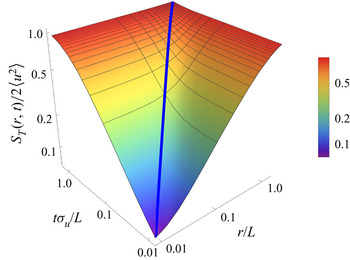
The result (A8) is shown in figure 15. We find the similarities between the results in figures 15 and 2 interesting. It is thus conceivable that many of the details in figure 4 can be explained by the sweeping motion caused by the large non-universal eddies.
Model results for the space–time-varying structure function. Since the model applies only to the inertial subrange, the figure is restricted to  $r\geq \eta _0$ and
 $t\geq \tau _K$. The solid blue line gives
 $r = \sigma _u t$.

The analysis of Kofoed-Hansen & Wandel (Reference Kofoed-Hansen and Wandel1967) allows also an estimate of the Lagrangian structure function. The result turns out to consist of simply replacing  $\sigma _u$ by
 $\sigma _u\sqrt {2}$. We analysed also this case using the model spectrum (A3). The observed time variation was
 $\sim t^{2/3}$ and in noticeable disagreement with that in figure 6.
As far as the inertial subrange is concerned, it makes no substantial difference to distinguish the component spectra and the full summed spectrum and corresponding structure functions. By the choice of the von Kármán spectrum we illustrate here a systematic and physically plausible transition to the large-scale non-universal energy-containing eddies for  $k\rightarrow 0$.
The present model could in principle be generalized to include a viscous subrange. There is, however, no universally accepted spectral model that includes such a viscous subrange.
A.2. Filtered, scale-size-dependent advection velocities
A.2.1. The Eulerian case
In the foregoing section it is implicitly assumed that all scales are advected with the same velocity. In reality an eddy with characteristic size  $D$ is advected by scale sizes
 $\geq D$ (Csanady Reference Csanady1973; Mikkelsen et al. Reference Mikkelsen, Larsen and Pécseli1987), while smaller scales distort the eddy. This argument can be expressed in terms of wavenumbers by letting
 $D \sim 1/k$. At a wavenumber
 $k$ the sum of component power spectra
 $\mathcal {E}(k)$ entering (A6) will contain contributions from all wavelengths
 ${\leq }\,2{\rm \pi} /k$ due to the aliasing. At any given
 $k$ we can account for the advection caused only by the larger scales by introducing a filtered power spectrum
 $u_f^2(k) = \int _0^k \mathcal {E}_K(\xi )\,\textrm {d}\xi$ replacing
 $\sigma _u^2$. For very large wavenumbers (small scales) the filter gives approximately
 $\sigma _u^2$ while small
 $k$ gives
 $({11}/{9}) (k L)^5 ( \varGamma (5/6) / \varGamma (1/3) \sqrt {{\rm \pi} } ) \sigma _u^2 \approx 0.3 (k L)^5 \sigma _u^2$. The result for filtered, or scale-size-dependent, velocities is shown with a heavy dashed line in figure 14. The structure function is now only approximately following a simple power law, and here with an exponent smaller than
 $2/3$, closer to
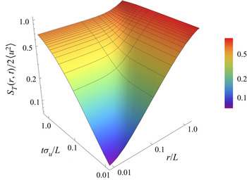
 $1/2$. The model result is now in better agreement with the numerical results found in figures 10 and 11, keeping in mind though that those contain also the viscous subrange. The spatially varying structure functions shown in figure 1 are not affected by this filtered advection. A summary of the results for the full space–time variation of the structure function is found in figure 16. The overall features remain the same as in figure 15. The modifications due to the filtering are modest for
 $r \ge \sigma _u t$, while differences are found in the details for
 $r < \sigma _u t$.
Model results for the space–time-varying structure function corresponding to figure 15, here using a velocity filter accounting for scale-size-dependent velocities.

The present velocity-filtered model opens the possibility of a  $\sim t^{2/3}$ inertial subrange also for the time-varying Eulerian structure function, but only if a time range
 $\tau _K\ll t\ll L/\sigma _u$ can be realized. This is not the case for the present numerical simulations.
As an additional illustration of the properties of the filtered KHW model, we show in figure 17 results obtained by sampling the structure function along a line  $t = r/V$ and then changing the plotting variables as in figures 8 and 9. Comparing figures 8, 9 and 17 we keep in mind that the KHW model in its form used here contains only the inertial subrange. Also for the KHW model we find a saturation as
 $V$ increases, although here the requirement appears to be more restrictive, i.e. the model requires
 $V/\sigma _u \geq 3$ before we can argue that
 $\mathcal {S}(r,r/V) \approx \mathcal {S}(r,0)$. The general features of figures 8, 9 and 17 are the same: the curves for
 $\mathcal {S}(r,r/V)$ increase and move towards smaller
 $r$ values as
 $V$ decreases. Also we find a slow systematic decrease in the average slope of the structure function as
 $V$ is decreased.
Model results (in a double logarithmic presentation) for samples of the Taylor hypothesis applied to the filtered version of the KHW structure function using  $V/\sigma _u = 1/8$, 1/4, 1/2, 1, 5/2, and 10 from top to bottom, to be compared with figures 8 and 9. The dashed line gives the slope of
 $r^{2/3}$ for reference.

A.2.2. The Lagrangian case
The KHW result for the Lagrangian structure function (see figure 18) is not promising by giving a  $t^{2/3}$ form for the time variation in a large time interval, different from the numerical results in figure 6 and in disagreement also with (2.2). We believe the mistake to be that the KHW model includes an advection velocity in the Lagrangian model in the same way as in the Eulerian case. The temporal variations in the Eulerian case are in part caused by small eddies advected past the fixed observer by the large energy-containing eddies (Tennekes & Lumley Reference Tennekes and Lumley1972). A Lagrangian co-moving observer will not observe similar time variations. In this case the observed time variations are due to eddies moving with respect to each other and to eddy deformations. A characteristic eddy velocity for an eddy of size
 $\ell$ can be formed by dimensional reasoning as
 $u_e\sim (\epsilon \ell )^{1/3}$, which can be expressed in terms of wavenumbers by the replacement
 $\ell \sim 1/k$. A more detailed eddy velocity model (Orszag Reference Orszag1977) corresponding to an eddy of scale size
 $1/k$ can be derived from the power spectrum as
 \begin{equation} u_e(k) =\sqrt{ \int_{\frac{1}{2}k}^{2k} \mathcal{E}_K(\kappa) \,\textrm{d}\kappa }, \end{equation}
albeit with an ad hoc choice of the eddy definition (Orszag Reference Orszag1977). A change in definition will only give rise to a change in a numerical coefficient. The effects of the detection point moving along a Lagrangian orbit together with an eddy in a surrounding of other eddies with other velocities can be described by the replacement  $u^2_{rms}\rightarrow u_e^2(k)$ in (A6). We recall that for incompressible homogeneous isotropic flows
 $\langle u^2\rangle$ is the same, irrespective of Lagrangian or Eulerian samplings being used. The Lagrangian structure function is shown with a dashed heavy line in figure 18. We find a clear
 $\sim t$ variation, in agreement with (2.2). Since
 $u_e^2(k) < u_f^2(k)$ for all
 $k > 1/L$, we can conclude that the Lagrangian integral time scale is here larger that its Eulerian counterpart. This is at variance with results obtained by, for instance, Weinstock (Reference Weinstock1976).
Model results for the Lagrangian structure function. The solid line gives the result found by Wandel & Kofoed-Hansen (Reference Wandel and Kofoed-Hansen1962) and the thick dashed line is the one suggested in the present analysis. The two thin dashed lines give the reference slopes of  $t^{2/3}$ and
 $t$, respectively.

The model illustrated in the present appendix is restricted by assuming all observed time variations to be caused by advection of eddies. Nonetheless it is found that the results can be brought into fair agreement with those of the numerical simulations, in particular when the filtered advection velocity is applied. One basic feature of the KHW model is retained in its filtered version: it derives all time variations (both Eulerian and Lagrangian) from the wavenumber spectrum alone. The present results are based on a von Kármán spectrum in order to have a well-defined outer scale. Due to the periodic conditions used in the simulations, that part of the simulation results differs from the von Kármán spectrum. The analysis here can readily be generalized to two-dimensional turbulence, but for that case (A8) has to be modified (Pécseli & Mikkelsen Reference Pécseli and Mikkelsen1985; Pécseli & Trulsen Reference Pécseli and Trulsen1995).
Appendix B. Approximations for structure functions
We have analytical expressions for the structure functions for the two universal subranges, the inertial and the viscous. There seems to be no analysis covering both ranges, but we can give a phenomenological expression and test it against the data. It turns out that it is possible to give a very satisfactory model.
Assume that we have an experimentally or numerically determined monotonically increasing (decreasing) function  $F(y)$ with functional forms
 $F_1(y)$ and
 $F_2(y)$ for small and large values of the variable
 $y$, respectively. The function
 $F$ can be approximated by a class of curves of the form
 \begin{equation} F(y) = \frac{F_1(y)F_2(y)}{(F_1^p(y) + F_2^p(y))^{1/p}}, \end{equation}
where  $p$ is an adjustable transition parameter, not necessarily an integer. We use this model for approximating the Eulerian and also the Lagrangian structure functions. For the Eulerian case with
 $y = r$, we have
 $F_1(r) = C_1 r^2 \epsilon /\nu$ and
 $F_2(r) = C_2 (r \epsilon )^{2/3}$ and find that the choice
 $p = 5/4$ gives an excellent fit as shown in figure 1. The coefficients
 $C_1$ and
 $C_2$ are determined through least squares fitting to take values 0.062 and 1.924. These should be compared with
 $C_\nu = 1/15 \approx 0.0667$ and
 $C_K$. A Fourier transform of the correlation function obtained from the fitted curve in figure 1 reproduces a subrange following the spectral Kolmogorov–Obukhov
 $5/3$ law.
The approximation inherent in (B1) can always be used, but there is no a priori reason for it to be particularly good, so the observed fine agreement deserves attention. In a previous study (Pécseli et al. Reference Pécseli, Trulsen, Stiansen and Sundby2020) we gave an analytical approximation using  $p = 1$, but found that the choice mentioned before is more accurate. The difference between the values of
 $C_1$ and
 $C_\nu$ may be due to an upper wavenumber limit for the viscous subrange in the numerical solutions. It could also be due to the increased statistical uncertainty of the numerical result at small
 $r$ values.
Analytical approximations can be given also for the results shown in figures 10 and 11. With  $F_1 (t) = C_1 t^2$ and
 $F_2 (t) = C_2 t^{1/2}$ and proper choices of the constants
 $C_1$ and
 $C_2$, and using
 $p = 1$, we find the analytical curves shown with thin red lines in figures 10 and 11.
An approximation for the Lagrangian structure function over the entire universal range in figure 6 can be obtained as well. With  $F_1(t) = C_1 t^2$ and
 $F_2(t) = C_2 t$, using
 $p = 5/2$ we obtain the result given by the thin red curve in figure 6. For the normalized Lagrangian counterpart of the structure function (see figure 6), we found
 $C_1 = 12.677$ and
 $C_2 = 9.101$.
The Lagrangian structure function differs from the Eulerian one by showing a trend towards the constant asymptotic limit within the available  $r$ range. The green (partly underlying) curve in figure 6 is the result of using the expression (B1) a second time with
 $F_1$ set equal to the universal range approximation (the thin red curve),
 $F_2 = 2u_{x,rms}^2$ and
 $p = 2$.