2.1. Air Force Research Laboratory M6LT

The partially closed cavity (PCC) experiments were performed in the Air Force Research Laboratory Mach-6 Ludwieg Tube (AFRL M6LT). A detailed description of the facility can be found in Kimmel et al. (Reference Kimmel, Borg, Jewell, Lam, Bowersox, Srinivasan, Fuchs and Mooney2017). This hypersonic wind tunnel, operating at typical noise levels for a conventional hypersonic facility, provides a low-enthalpy environment that allows for efficient and rapid experimental runs across a range of Reynolds numbers. To ensure consistent test conditions, the stagnation temperature is maintained near 505 K via preheating of the compressed air and maintaining that temperature via wrapping the driver tube in thermal blankets. A fast-acting valve positioned upstream of the nozzle enables multiple tests to be conducted in rapid sequence, removing the need to replace diaphragms between runs. Large (304.8 mm) windows on either side of the test section provide optical access suitable for techniques such as schlieren and interferometry. An additional, smaller overhead window allows for diagnostics like infrared thermometry and other laser-based measurement techniques.

The AFRL M6LT is capable of operating with stagnation pressures ranging from 0.35 to 4.00 MPa, resulting in unit Reynolds numbers between 2.2 and 30.1 million per metre. Each test cycle provides two periods of quasi-steady Mach-6 flow, each lasting approximately 100 ms, before the tunnel experiences unstart. While not a quiet tunnel, the AFRL M6LT exhibits relatively low free-stream noise, with root-mean-square pitot pressure fluctuations below 3 % of the mean pitot pressure. The reported experiments were performed at a Mach number of approximately 6.1.

2.2. Partially closed cavity model

The PCC model was designed to facilitate the experimental investigation of instabilities associated with a forward-facing door over a hypersonic cavity. Note that in this case ‘partially closed’ refers to the geometry of the test article, as opposed to the aerodynamic category of the cavity flow. This model, illustrated in figure 1, consists of a flat plate with a rectangular cavity positioned 184.9 mm downstream of the leading edge. The cavity measures 152.4 mm in length (streamwise direction) and 73.7 mm in width (spanwise direction). A key feature is the inclusion of a hinged door, allowing for variations in the cavity opening angle, denoted as $\theta$ in figure 1. The door has a flat, 3.208 mm-wide leading edge with 0.406 mm x 45.00 $^\circ$ chamfers along its upper and lower edges. The cavity depth, $D$ , can be adjusted by vertically translating the floor, enabling aspect ratio ( $L/D$ ) variations. For optical access, the cavity walls are constructed from 9.65 mm thick fused silica windows. The model’s leading edge has a 1.25 mm radius of curvature, and the overall flat plat surface is 407.6 mm long by 269.9 mm wide.

Figure 1.

Illustration with streamwise dimensions in millimetres. Yellow indicates transparent sidewalls to provide optical access to the cavity. Flow is left to right.

The model incorporates several design features to enhance its experimental flexibility. Extensions on either side of the cavity, measuring 81.0 mm in width, are included to mitigate edge effects within the region of interest. An array of sensor ports, sized for PCB and Kulite pressure transducers, is integrated along the model surface downstream of the leading edge, along the upstream cavity wall and across the cavity floor. This arrangement allows for detailed surface measurements and characterisation of the flow field. Furthermore, the model accommodates the installation of various leading-edge configurations and trip strips, allowing for investigations into the influence of leading-edge geometry and surface roughness on the flow dynamics.

This study focuses on the centreline aerodynamics of the PCC with a smooth surface (no trip), with most measurements made for a cavity depth of 25 mm ( $L/D=6.1$ ). The model was installed at a −0.5 $^{\circ }$ angle of attack, positioning the upper surface on the windward side. The model and door angles were determined using a digital protractor after installation in the tunnel. Two experimental campaigns were conducted across a range of free-stream unit Reynolds numbers, spanning from $2.2\times 10^6$ to $13.6\times 10^6$ m⁻¹. The first campaign involved systematically varying the cavity-door angle between 2.5 $^{\circ }$ and 15 $^{\circ }$ , with the aim of simulating and analysing the flow phenomena associated with different stages of door opening in a Mach-6 flow. The second campaign included runs made with the door at a fixed angle of 7.5 $^\circ$ and the cavity depth varied between 15.0 and 35.0 mm ( $L/D$ between 10.16 and 4.35). The depth was further extended to 50.4 mm ( $L/D=3.02$ ) in subsequent simulations to elucidate observed phenomena over an extended range not immediately accessible to the ground test. Photographs of the model as installed in the tunnel are shown in figure 2. Model locations described in this text are given with the origin assumed to be at the leading edge of the cavity.

The model was run without the door for a separate study (Benitez et al. Reference Benitez, Bisek, Borg, Clingenpeel, Molinaro and Meritt2026). The data from that test showed that the incoming boundary layer tended to be laminar with thicknesses just upstream of the cavity given in table 1. The values were estimated from schlieren imagery taken during the no-door experiment.

Table 1.

Estimated boundary-layer thicknesses immediately upstream of the cavity. Data obtained from schlieren imagery for the cavity model without the door installed (Benitez et al. Reference Benitez, Bisek, Borg, Clingenpeel, Molinaro and Meritt2026).

Figure 2.

Photograph of the PCC model installed in the AFRL M6LT with the cavity door set to 10.0 $^{\circ }$ . Upper image: looking downstream; lower image: flow is left to right.

2.3. Embedded sensors

A variety of different sensors were embedded in the model across two tunnel entries to collect data, with a focus on pressure-fluctuation measurements. Figure 3 shows the cavity floor and upstream model surface ports along with labels for the pressure sensors that were installed. The dashed lines show sensors installed during the first entry, which was focused on the effect of the door angle with a constant cavity depth of 25 mm. The solid lines are for sensors installed during the second entry, which was focused on the impact of cavity depth with a constant 7.5 $^\circ$ door angle.

Figure 3.

Illustration of pressure sensor installation locations for the PCC tests. Dashed lines represent sensors from entry 1, while solid lines are for sensors from entry 2. Only the upper model surface (beginning at the trip insert location) and the floor of the cavity are shown.

Surface pressure-fluctuation measurements were primarily acquired with Kulite XCE-062-15A sensors installed at various points along the test article. These sensors can capture both lower-frequency disturbances and static pressures, and have a 1.7 mm diameter. Due to a large resonance peak present near 300 kHz, their useful output is restricted to below 270 kHz. The Kulite sensors were calibrated by manually changing the test section pressure and recording voltages across a low-pressure range. For the calibration, the test section pressure is measured with a Mensor Type CPR2580 with an absolute pressure range of 0.0–33.0 psia. Several other sensor types were installed throughout the cavity floor and upstream surface of the model as well. These sensors include Piezotronics PCB 132B38 sensors and IC2 DynaMic EP-0120 sensors to also measure pressure fluctuations. The PCB sensors feature a nominal resolution of 6.89 Pa and a rise time of less than 3 $\mu$ s, enabling the capture of high-frequency pressure variations. With a high-pass filtering at 11 kHz and a high-frequency response limit of 1 MHz, these sensors are well suited for characterising the high-frequency content commonly found in hypersonic flows. The DynaMic sensors are designed to measure dynamic pressure fluctuations, and are characterised by a small form factor (3.18 mm diameter, 17 mm length). The sensors’ frequency response extends from 20 Hz to 115 kHz, and they have a sensitivity of 100 $\unicode{x03BC}$ V/Pa with a large dynamic range ( $\gt$ 128 dB). Additionally, both commercial and experimental sensors developed by Ahmic Aerospace to measure wall shear stress, temperature and heat flux were installed. All sensors were flush mounted. The large number of sensor types were included to see how they generally performed in the stressing conditions provided by this geometry and flow. However, only the Kulite results will be shared here.

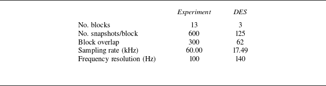
Time series data and power spectral densities (PSDs) are presented for the pressure data throughout the paper. For the experimental data, 70.0 ms of data were processed from the centre of the second quasi-steady period for each run. With the computational data, 14.3 ms of data were used for the analysis. Unless otherwise noted, the PSDs were computed using a frequency resolution of 100 Hz (equal to the sampling frequency divided by the window size). This corresponds to a window size of 175 for the detached eddy simulation (DES) data (which have a sampling frequency of 17.49 kHz for the data processing), while the experimental data have a window size of 20 000 (as they have a sampling frequency of 2.0 MHz); a Hamming window was used for both cases. The DES data were available up to 174.8 kHz, but based on experimental results, analysing every tenth frame was determined to be sufficient. Peak frequencies from the spectra were found by determining the midpoint between two frequencies of the same amplitude about the local maximum (see Benitez Reference Benitez2021) Appendix E.3 for more information and validation of this method).

2.4. Self-aligned focusing schlieren

Flow visualisation during the experimental campaign was achieved using a high-speed schlieren imaging system. A Photron Fastcam SA-Z-2100K-M-32 GB high-speed camera, operating at a frame rate of 60 kHz, captured schlieren images from a self-aligned focusing schlieren (SAFS) set-up. The SAFS diagnostic, originally described by Bathel & Weisberger (Reference Bathel and Weisberger2021) and implemented at the AFRL M6LT by Hill et al. (Reference Hill, Borg, Benitez, Running and Reeder2023), minimises the line-of-sight integration inherent in traditional Z-type schlieren systems. By adjusting the depth of focus, the turbulent shear layers originating from the tunnel nozzle exit were excluded from the imaging region. Illumination for the schlieren system was provided by a Cavitar Cavilux HF 640 nm pulsed laser with a pulse duration of 90 ns.

To facilitate quantitative analysis of the schlieren visualisations, an in-house MATLAB-based feature-tracking algorithm was utilised to track the separation shock present upstream of the recirculation region in the flow. The algorithm first pre-processes the raw images by subtracting a reference pre-run image. The directional gradient of the processed images is computed for a user-defined direction, enabling the identification of high-gradient regions by comparison with a given threshold. Outliers are removed by finding individual points greater than a user-defined distance from any other points. Additionally, the algorithm distinguishes points within and outside the designated region of interest. In the case of shock wave tracking, the algorithm fits lines to pairs of points within the region of interest and identifies the line with the most points along it as the shock. The linear fit results for each frame enable subsequent temporal analysis of shock fluctuations. Figure 4 shows an example of a single frame from the shock-tracking algorithm. The image shows the prerun-subtracted schlieren data for that particular frame overlayed with the algorithm-defined points. The red x symbols are points that exceed the gradient threshold but are outside of the defined range, while the blue + symbols are points that exceed the threshold inside the range. The user-defined range is bounded a polygon with vertices at the yellow squares. Diagonal striping that can be seen behind the model are from the prismatic retroreflective tape used with the SAFS configuration. The linear fit that the algorithm determined to be the shock is shown by an orange line. A manual investigation of the shock-tracking algorithm revealed it accurately captures the shock between 82 % and 98 % of the time depending on the particular conditions, with the inaccuracies generally caused by trendline jumps across features. To improve the accuracy, lines that jumped significantly between consecutive frames are removed from the output. Once the final set of lines is found, each line is extended to the model wall to find the shock-foot position where it intersects with the surface. Note that the true shock is not purely linear; it curves towards the surface of the model as it approaches the shock foot. By manually comparing the linear fit intersection with the true shock-foot location in the schlieren, it appears that the linear approximation results in a shock-foot location approximately 20–25 mm upstream of the true position.

Figure 4.

Example of the shock-tracking algorithm for the 7.5 $^\circ$ door angle and 25 mm depth case at ${\textit{Re}}_\infty =12.9\times 10^6$ m⁻¹, where ${\textit{Re}}_\infty$ is the freestream unit Reynolds number. Dimensions are in pixels.

Spectral proper orthogonal decomposition (SPOD) was also used to better visualise any aerodynamic instabilities present (Towne, Schmidt & Colonius Reference Towne, Schmidt and Colonius2018; Schmidt & Colonius Reference Schmidt and Colonius2020). This methodology allows for a mathematically optimal decomposition of spatio-temporally correlated structures in the images to be visualised. The normalised SPOD modal energies could also be analysed to see frequencies of significance present in the SAFS data. The SPOD is sensitive to several parameters, such as frame rate and the total number of frames. A large number of frames at a frame rate higher than the Nyquist frequency (twice the maximum measurable frequency) is necessary to resolve fluctuations in the SPOD modal energy. Table 2 summarises the SPOD parameters used for this study.

Table 2.

The SPOD parameters.

4.1. Experimental observations

The surface pressure data collected for the 7.5 $^\circ$ door-angle and 25 mm cavity-depth case included large fluctuations that occurred at approximately 500 Hz, regardless of sensor location. Figure 5 plots the time series data and PSD for one Kulite sensor located just upstream of the centre point on the cavity floor. The time series data, of which a subset is displayed in figure 5(b), include multiple cycles of static pressure measurements that rise from a minimum of approximately 1.2 kPa to a sharp peak of upwards of 80 kPa. This oscillation is strongly cyclic, with the primary peak in the PSD at 514 Hz having an amplitude of nearly two orders of magnitude above the floor and includes several clearly visible higher harmonics. Similar 500 Hz oscillations were apparent in all pressure sensors installed in the model, across both the upper surface and inside the cavity, although with different peak amplitudes. The universality of these oscillations in the experimental data indicate a likely global fluctuation of the flow.

Figure 5.

Time series data and PSD for the cavity-floor Kulite located $x=56$ mm downstream of the upstream cavity wall. Here, ${\textit{Re}}_\infty =13.6\times 10^6$ m⁻¹.

The strong 500 Hz fluctuations were apparent in the SAFS data as well. Figure 6 plots the results from a SPOD analysis for this experimental case from the SAFS data. The normalised SPOD modal energies (figure 6 a) are reminiscent of the Kulite PSD from figure 5(c). Sharp peaks are observed starting at 500 Hz in the first SPOD mode. The normalised amplitude is near one for the primary peak as well as the first several harmonics, indicating that nearly all the SPOD energy is contained in that mode for that frequency. Mode shapes for the 500 and 1000 Hz mode-one cases are plotted in figure 6(b) from the real part of the leading SPOD mode. The 500 Hz case corresponds to the dominant instability measured in the flow, while the 1000 Hz case relates to its first harmonic. The appearance of harmonics from the dominant instability was validated by a bicoherence analysis (see figure 7b from Benitez et al. Reference Benitez, Borg and Khattar2025). For both frequencies, much of the non-zero components are congregated above the upstream model surface, as well as around and just below the leading edge of the door. The SPOD results provide evidence that the 500 Hz oscillations are not just a surface pressure phenomenon, but extend outward into the flow around the model.

Figure 6.

The SPOD modal energies and mode shapes from the SAFS data. Here, ${\textit{Re}}_\infty =13.6\times 10^6$ m⁻¹.

The instantaneous SAFS imagery was used to help decipher the source of the strong 500 Hz fluctuations. A sample of frames spanning one complete cycle is shown in figure 7. The instantaneous mean-subtracted schlieren frames were extracted every $0.2$ ms. Figure 7(a–e) shows the cycle half-period where the bubble is expanding, starting with it at its smallest size. It begins with figure 7(a), where the bubble separation shock and shear layer are both located below the door. The shear layer interacts with the door bow shock, causing a similar phenomenon to a type-IV shock-shock interaction (Albertson & Venkat Reference Albertson and Venkat2005). A strong jet is formed from this interaction (circled in grey), which impinges on the door, likely deflecting mass into the cavity. The cavity begins to fill, which leads to an increase in the bubble size. As the bubble grows in figure 7(b), the separation shock shifts upstream, moving to impinge on the leading edge of the door. The jet increases in strength, now clearly reflecting off the door and into the cavity, with the jet in the cavity directly observable in the SAFS imagery (circled in grey). Expanding further into figure 7(c), the separation shock moves above the door, now creating a type-V shock-shock interaction (circled in grey). The door bow shock appears to warp near the intersection, with a bulge in the upstream direction and a jet emanated out from that point. The shear layer above the bubble now begins to transition from laminar to turbulent (transition point at the grey dot) and reattaches at the door leading-edge. There is still a deflection of mass into the region under the door. By figure 7(d), the separation shock is now well above the door, although still interacting weakly with the bow shock (likely a type-VI interaction). The shear layer transition point has shifted upstream (grey dot), and downstream of it the shear layer begins to broaden in height. In figure 7(e), the bubble is nearing its maximum size, with the separation shock crossing the door bow shock near the upper edge of the schlieren field of view. By this frame, the shear layer is fully turbulent, and continues to broaden in height as it moves downstream. At the leading edge of the door, the shear layer is so thick that its mass moves partially above and partially below the door (grey circle). This relief causes the bubble to cease to grow.

Figure 7.

Instantaneous, mean-subtracted schlieren montage for the 7.5 $^{\circ }$ door angle and 25 mm cavity depth at ${\textit{Re}}_{\infty }=13.6\times 10^6$ m⁻¹ showing separation bubble expansion and collapse over time. One frame is displayed every 12 samples across 2 ms (0.2 ms between frames).

Figure 7(f–j) documents the half-cycle where the bubble collapses, starting with it at its largest size. The first frame (figure 7 f) occurred $0.2$ ms after figure 7(e). The bubble collapse appears to be similar to the expansion but in reverse, with the separation shock receding towards the cavity. At its largest (figure 7 f), the bubble appears to separate near (but still downstream of) the leading edge. The shear layer appears almost entirely turbulent. The bubble appears to hold this position through the next frame (figure 7 g), with the shear layer mostly flowing over the top of the door. By figure 7(h), the turbulent shear layer has started to retract downward, and is now centred at the door leading edge. As the bubble contracts, the separation shock shifts downstream in figure 7(i–j). The shear layer becomes laminar for the upstream third of the bubble before transitioning to turbulence at the grey dot in figure 7(i). This pattern continues into figure 7(j), with a laminar shear layer for the first half of the bubble. The separation shock fades out from the SAFS imagery as the bubble nears its minimum size. By figure 7(j), the shear layer returns to being fully below the door. The shear–shock interaction again develops a supersonic jet that impinges on the door and deflects mass into the cavity, repeating the cycle once more.

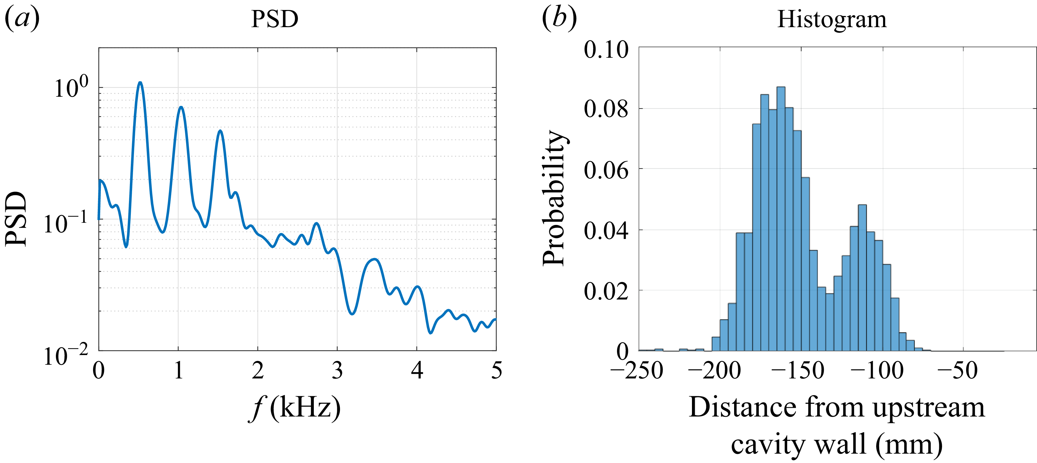
Using an in-house shock-tracking algorithm (see § 2.4), the shock-foot location was extracted from the SAFS data for the separation shock upstream of the cavity. Note again that due to the assumption of a linear shock, the true shock-foot location is likely 20–25 mm upstream of the positions given here. This metric is correlated with the separation point for the recirculation bubble, providing information about the bubble’s behaviour during each cycle. Figure 8 plots the PSD and histogram for the shock-foot position, determined in millimetres from the upstream cavity wall. From the PSD, a strong peak is present at 521 Hz, along with two harmonics clearly visible above the noise floor. This peak, less than 1.4 % off from the Kulite peak frequency, tracks with the fluctuations measured in both the surface pressure sensors and the SAFS SPOD analysis. The histogram reveals an interesting bimodality in the data. Rather than a Gaussian distribution of shock-foot locations centred on the mean, there are two distinct peak positions. This result is indicative of dynamic behaviour centred about two locations, where the separation point has a sinusoidal pattern with the bubble being one of two sizes for most of the cycle.

Figure 8.

The PSD and histogram of separation shock-foot location relative to the upstream cavity wall, from SAFS data. In the histogram, the upstream cavity wall would be at $x=0$ mm. Here, ${\textit{Re}}_\infty =12.9\times 10^6$ m⁻¹.

Given unsteadiness that has been observed with other shock/boundary-layer interactions (SBLIs) (Clemens & Narayanaswamy Reference Clemens and Narayanaswamy2009), the approximately 515 Hz frequency was normalised to see if it aligned with the Strouhal numbers ( $St$ ) observed in other SBLI studies. The computed edge velocity of approximately 875 m s⁻¹ was used as the characteristic velocity, while several characteristic lengths were attempted. However, all of the estimates were outside of the 0.01–0.03 Strouhal numbers generally measured for SBLIs (Clemens & Narayanaswamy Reference Clemens and Narayanaswamy2009), indicating that the PCC fluctuations are likely independent of that SBLI instability. It is also notable that the SBLI fluctuations are generally measured for turbulent SBLIs, while the incoming boundary layer is mostly laminar or transitional for this case.

It was investigated whether the 515 Hz oscillation could be accounted for by established empirical models. For the configuration tested, fluctuations at 464 Hz were predicted by the Rossiter mechanism, seeming to show reasonable agreement. However, when the model was expanded to estimate fluctuations for cavities of different depths (see § 5.2), peak frequencies varying by several hundred Hertz were predicted, a variation that was not observed in the experiments. Given the observed cycles’ resemblance to supersonic inlet buzz, an organ-pipe calculation was also attempted. With estimated frequencies of 200–400 Hz depending on the representative length selected, satisfactory agreement was not achieved. Finally, a closed-box empirical method was tried (Ünalmis et al. Reference Ünalmis, Clemens and Dolling2004), resulting in a frequency of 479 Hz. This method agreed the best with the experiment, but does not include a dependence on cavity depth, which was shown to impact the peak frequencies experimentally (as described in § 5.2).

4.2. Computational study

A DES was run for the full-span, no-wing, 7.5 $^\circ$ -door configuration with ${\textit{Re}}_\infty =12.9\times 10^6$ m⁻¹. The results from this simulation were compared with the experimental results and further analysed to better understand the overall physics of the flow by analysing parameters that cannot be measured experimentally.

4.2.1. Comparison with experimental results

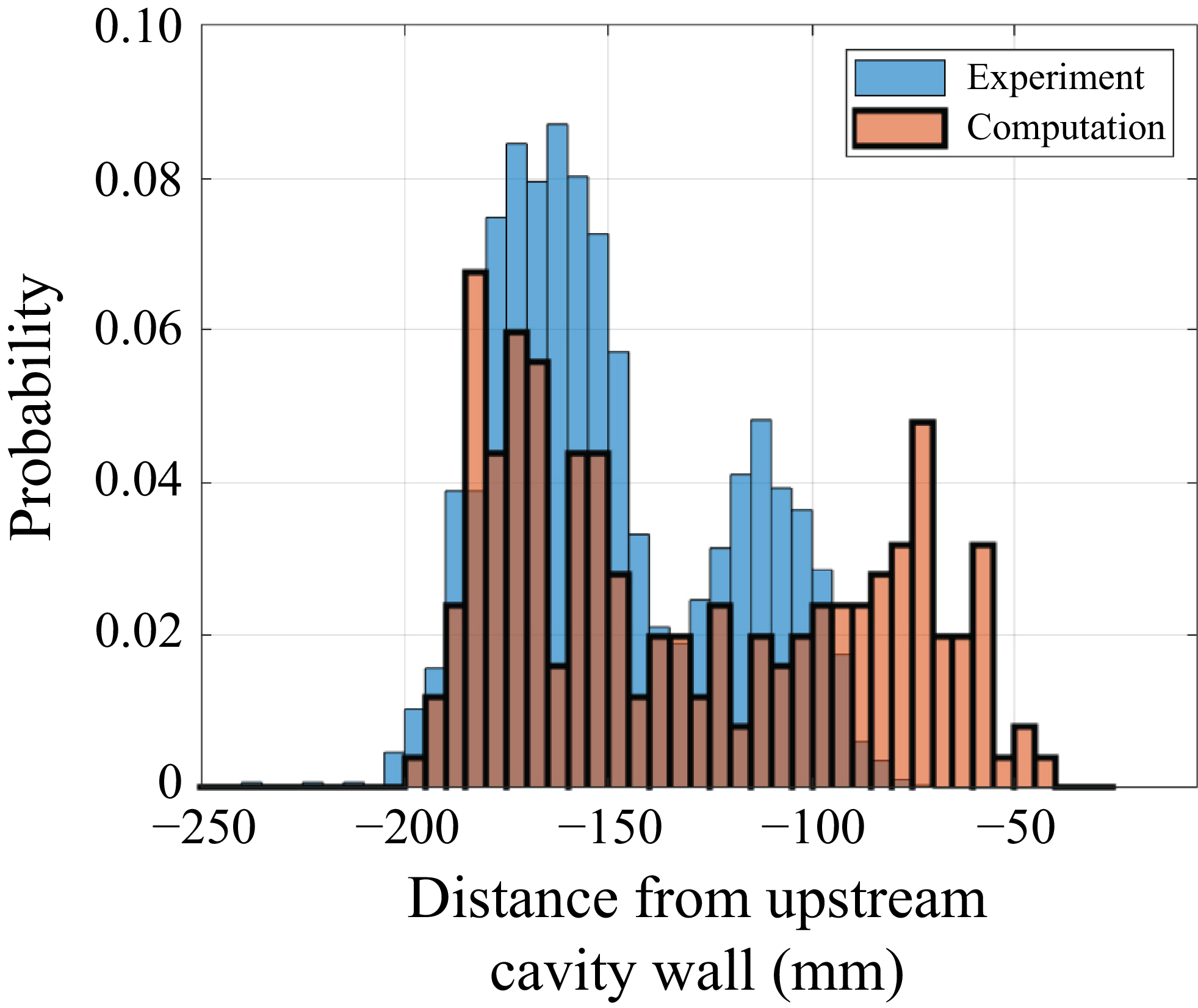
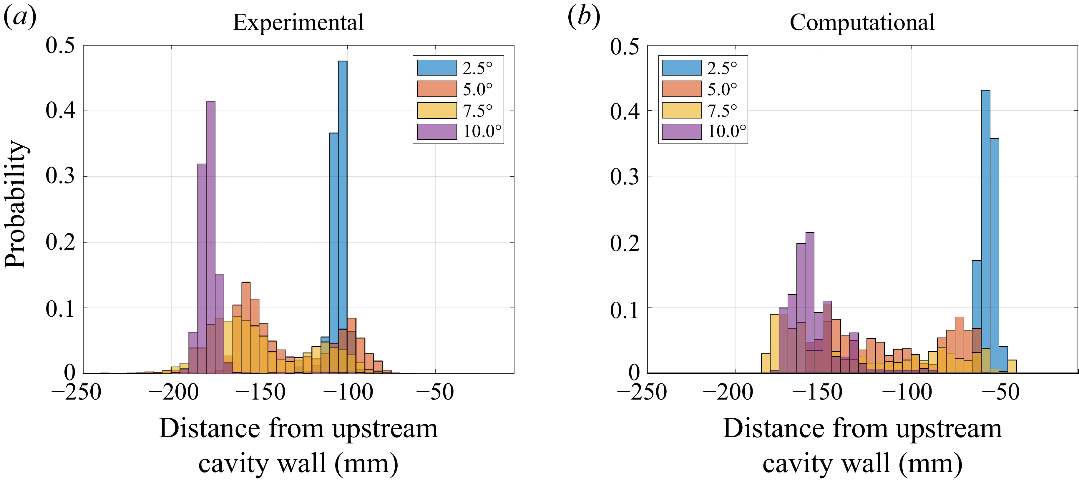
Pseudo-schlieren images were created from the computational results by plotting the density y-gradient of the DES solution along the centreline plane. The pseudo-schlieren images were then run through the same shock-tracking algorithm that was used on the experimental SAFS data. The histograms of shock-foot positions from this computational case are shown with the experimental results in figure 9, with the horizontal axis representing the shock-foot position in millimetres from the upstream cavity wall and the vertical axis representing the probability of the shock foot being at that particular position. Note once more that due to the assumption of a linear shock, the true shock-foot location is likely 20–25 mm upstream of the positions given here. The DES histogram is bimodal, similar to the experimental results, with the upstream mode being centred around the same position (approximately −170 mm). However, the computational results have more spread, with the downstream modal peak centred around −75 mm, while the experimental peak is near −115 mm. This difference between the computational and experimental shock-foot distributions may be due to a discrepancy between the computational and experimental measurements, but more likely appears to be an artefact of the shock-tracking algorithm. The DES data were much cleaner than the experimental data, without any background fluctuations and with constant positive or negative values in the shock or shear layers. This allowed the algorithm to more accurately pick out the separation shock without any confusion with the door bow shock or the separation bubble shear layer. With the experimental data, the algorithm had to be artificially constrained to a more limited region of the flow to avoid switching between the true separation shock and the bow shock about the door or the shear layer above the bubble. This limitation for the experimental data prevented the separation shock from being located as far downstream as the DES results were found to be. Visually observing the SAFS and pseudo-schlieren videos, the extent of the bubble appears to be approximately the same between the two sets of results.

Figure 9.

Shock-foot position comparison including the DES results. The upstream cavity wall would be at $x=0$ mm. Here, ${\textit{Re}}_\infty =12.9\times 10^6$ m⁻¹.

The pseudo-schlieren imagery could also be used to run an SPOD analysis of the computational data. Note that, due to the different sampling rate and total number of frames relative to the experimental results, slightly different SPOD parameters were necessary (see table 2). Despite those differences, the computational SPOD results were remarkably similar to the experimental one. Figure 10 plots the normalised SPOD modal energies and two SPOD mode shapes obtained with the DES pseudo-schlieren. The normalised modal energies, plotted in figure 10(a), show the three SPOD modes obtained from the DES analysis (with solids lines) as well as the first SPOD mode from the experimental data (with a light-red dotted line). The first SPOD mode from both the experiment and the computational agree very well, with the first peak aligning in both frequency and normalised amplitude. The mode shapes for the frequencies at 420 and 980 Hz (frequencies closest to the interpolated peak frequencies from SPOD results) are also qualitatively similar to the experimental mode shapes, with strong fluctuations apparent near the leading edge of the door. Note that slightly different mode-shape frequencies were extracted from the computation compared with the experiment due to the different SPOD parameters required by the shorter time series as compared with the experimental data. Black contours of the nearest experimental mode shapes are overlaid on top of the computational mode shapes in figure 10(b). The experimental contours align well with the major features of the computed flow, such as the shocks, shear layer and jet. The computational shapes differ in that the region of the bubble sweep above the upstream model surface is more distinct, and the jet deflected into the cavity is also clearer in these results, likely due to the less-noisy imagery from DES as compared with the experiment.

Figure 10.

The SPOD modal energies and mode shapes from the DES data; SPOD mode 1 normalised energy and mode shapes from the experiment are also included for comparison. Here, ${\textit{Re}}_\infty =12.9\times 10^6$ m⁻¹ for the DES and $13.6\times 10^6$ m⁻¹ for the experiment.

A more quantitative comparison between the experimental and computational tests is shown in figure 11. The experimental and computed static pressure measurements were extracted at the cavity floor at three streamwise positions along or near the centreline: 6, 56 and 96 mm downstream of the upstream cavity wall (or 187, 237 and 277 mm downstream of the model leading edge). These positions are shown as red circles along the cavity floor in figure 11(a). The experimental data were measured with a Kulite XCE-062 sensor, while the DES data were extracted from a single point located at the centre of the Kulite sensor face. The DES data were shifted in time to align the first cycle with the experimental data displayed in the plots. As can be seen in figures 11(b), 11(d) and 11(f), the experimental and computational data series agree extremely well. For the 6 mm point (near the upstream corner of the cavity), peak pressures reached between 10 and 13 kPa. At the 56 mm position (just upstream of the cavity centre point), the maxima were between 30 and 75 kPa and at 96 mm (just downstream of the cavity centre) they were between 15 and 25 kPa for both sets of data. The minima for all three locations were between 1.0 and 1.5 kPa for both the computational and experimental data. The pressure peaks have comparable widths between the experimental and computational results, with sharp, narrow peaks at 56 mm and wider peaks at 6 and 96 mm, and have similar periods. Power spectral densities for the two data sets are shown in figures 11(b), 11(d) and 11(f). The PSDs have peak frequencies less than 6 % apart, with the computational and experimental data having peaks at 488 and 514 Hz, respectively. The peak amplitudes, however, vary more. It is important to note that the DES results contained a total of 7 pressure cycles, while the experimental results included 36, likely accounting for some these differences in peak amplitudes.

Figure 11.

Time series (b, d, f) and PSDs (c, e, g) for the experimental and computational data from three Kulite sensors located on the cavity floor at the positions marked in (a). The Kulites were positioned along or near the centreline 6 (b–c), 56 (d–e) and 96 mm (f–g) from the upstream cavity wall. The 6 mm Kulite data and all CFD data were at ${\textit{Re}}_\infty =12.9\times 10^6$ m⁻¹, while the 56 and 96 mm Kulite data were at ${\textit{Re}}_\infty =13.6\times 10^6$ m⁻¹.

Figure 12 plots histograms for the experimental and computational data at three streamwise positions along the centreline of the cavity floor (figure 12 a–c), and for the computational data across the full cavity floor (figure 12 d). The axial locations are again at $x=6$ , $56$ and $96$ mm downstream of the upstream cavity wall for the three Kulite sensors (figures 12 a, 12 b and 12 c, respectively; positions marked with grey dashed lines in figure 12 d). The experimental histograms show static pressure on the horizontal axis, and the probability that a given pressure is measured along the vertical axis. Two of the three sensor locations (6 and 96 mm) show seemingly bimodal distributions, with a narrow high-probability low-pressure peak and a wider lower-probability but higher-pressure peak. At 6 mm downstream of the cavity edge, the low-pressure peak is around 1.8 kPa, while the high-pressure maximum is near 5.3 kPa. The computational distribution at that position is plotted on top with an orange line. Computationally, the low-pressure peak was at a lower pressure than from the experiment, and a high-pressure plateau can be observed at a slightly higher pressure. The overall distribution shape, however, generally agreed. At 96 mm, there is more spread, with the low-pressure peak around 1.2 kPa and the high-pressure one near 11 kPa in the experiment. The computational distribution again has a similar shape at that location. The 56 mm point differs from the other two with a single clear peak, although at a lower peak amplitude. This peak occurs near 1.6 kPa, but has a long high-pressure tail that extends out past 80 kPa.

Figure 12.

Histograms for the experimental data at three streamwise positions along the centreline of the cavity floor, and for the computational data across the full cavity floor. Positions are in millimetres downstream of the upstream cavity wall. The axial locations are $x=6$ , $56$ and $96$ mm downstream of the upstream cavity wall for the three Kulite sensors (marked with grey dashed lines on the CFD plot).

The full-cavity computational results are presented as a contour map where the probability is based on the colour intensity and the vertical axis shows position downstream of the upstream cavity wall, in millimetres. The pressures were averaged over the central 25 mm in span and displayed for each axial position along the cavity. Probabilities of zero are blanked to allow for visualisation of the long low-probability but high-pressure tails present for some positions. The DES results show a similar trend to the experimental histograms, with a broader peak and potential bifurcation near the upstream corner, a single peak with a long high-pressure tail near the centre, and a clear bifurcation in the peak pressure across the downstream third of the cavity. The peak pressures at the three Kulite positions agree well with the values from the sensor histograms. The computational plot helps elucidate the overall trends across the cavity floor, showing where the jet impingement creates high peak pressures around the 56 mm point, resulting in pressure traces that have a narrow, high-amplitude peak. The bifurcation along the downstream region demonstrates the repeatable sinusoidal pressure oscillations that were observed in the time traces from that region.

4.2.2. Oscillation mechanism analysis

The excellent agreement between the experimental and computational static pressures provides confidence in the DES results, which are now used to improve understanding of the aerodynamics underlying the observed oscillations. Figure 13 shows pressure data from five locations along the centreline of the cavity floor, with time series plotted in figure 13(b) with an enhanced view in figure 13(c). The locations are located 6, 56, 76, 96 and 147 mm downstream of the upstream cavity wall; the 6, 56 and 96 mm positions correspond to axial locations of Kulite sensors, while the 76 mm point is directly at the centre of the cavity and the 147 mm position is near the downstream corner of the cavity opposite the 6 mm location. The data were taken at each location without the spanwise averaging used in the histogram plots. Note that the 6 mm position was obtained during a different tunnel entry than the other two locations; since an exact match for ${\textit{Re}}_\infty$ was not available, the run with the closest condition was used instead. From these figures, the upstream corner of the cavity appears to contain a much more quiescent region than the other locations. The minimum pressure of all five locations is between 1.0 and 1.5 kPa. While the upstream corner’s peak pressure reaches up to 12 kPa, the downstream corner’s peak fluctuates to 26 kPa, and the centre locations’ peaks shift to anywhere between 28 and 70 kPa. The centre (76 mm) and downstream (147 mm) locations begin to rise at approximately the same time, with the other three positions delayed relative to them. This simultaneous rise is due to the initial jet formation (for the 76 mm location) and air compression at the end of the cavity (for the 147 mm one), the effects of which are delayed for the other locations. However, all five positions appear to begin to decrease in pressure at the same time. The 6 and 96 mm positions maintain their low-pressure value for a finite period of time before increasing, reaching a peak and decreasing again. The downstream (147 mm) location has a square-wave-like shape, with the pressure fluctuating between a lower value and a consistent upper plateau. The centre (76 mm) location is at its minimum pressure for less time than the upstream location, but about the same amount of time as the downstream one. It rises to an initial peak, drops briefly before spiking to its maximum and then dropping again. It then fluctuations across a roughly 1 kPa span until it begins to decrease in pressure at the same time as the other two location. Just upstream of the centre, the 56 mm location has similarly high peaks with erratic fluctuations, but its peak is delayed relative to the 76 mm location. This delay is due to the forward-sweeping motion of the supersonic jet, as will be discussed below.

Figure 13.

Time series for the computational data along the centreline of the cavity floor. The axial locations are $6$ , $56$ , $76$ , $96$ and $147$ downstream of the upstream cavity wall; sensor location circles match their associated time series line colours. Here, ${\textit{Re}}_\infty =12.9\times 10^6$ m⁻¹.

The enhanced view of a single cycle for each of the five positions from figure 13 is plotted in figure 13(c). Six dashed black lines (labelled $a$ through $f$ ) highlight interesting features from the pressure traces that are expanded upon in the following figures. Line $a$ marks the initial peak for the centre (76 mm) and downstream (147 mm) positions, when the remaining points are still at their minimum pressure. Line $b$ is when the centre point reaches its overall maximum, while the upstream (6 mm) point is still at the minimum pressure and the downstream (147 mm) point is along its high-pressure plateau. At this time, the 56 and 96 mm positions are beginning to rise in pressure. Next at line $c$ , the centre pressure has dropped back down and is in the local minimum that occurs after it reaches its maximum peak, while the 56 mm point is reaching its maximum pressure peak. The 96 mm point is roughly linearly increasing in pressure. The upstream (6 mm) position has started to rise slightly, while the downstream (147 mm) position is still maintaining its high-pressure plateau. Line $d$ occurs when the pressure rises again at the centre point and is at a local minimum for the 56 mm location. It is still continuing to rise at the 6 and 96 mm positions and stay along the plateau for the 147 mm position. All five points begin to decrease in pressure at line $e$ . Finally, line $f$ occurs during the minimum pressure for all five positions.

To help elucidate the aerodynamic mechanism behind the pressure fluctuations documented in the previous figures, pseudo-schlieren images (density $y$ -gradient slices) along the centreline are plotted in figure 14. Each figure is labelled with the corresponding line from figure 13(c) indicating each key point in time, and the location of each of the five positions for the cavity-floor pressure measurements is shown as a red circle. In figure 14(a), the large separation bubble upstream of the cavity is in the middle of collapsing. The separation shock, circled in solid grey, is approximately one third of the way downstream between the leading edge and upstream cavity wall. The shear layer, circled in dashed grey, intersects the bow shock from the door, initiating the formation of the jet (circled in dotted grey) that deflects flow into the cavity. This deflection mostly goes near the centre of the cavity, resulting in the initial peak for the centre position in figure 13(c) at line $a$ . By figure 14(b), the bubble has collapsed further, and a jet (dotted grey) has clearly developed at the intersection of the shear layer (dashed grey) and the door bow shock. The separation shock (solid grey) appears more diffuse and intersects with the door near the leading edge. Interestingly, the shear layer (dashed grey), and not the separation shock, is the cause of the jet, indicating it is likely due to a shear–shock interaction rather than a shock–shock interaction as initially thought from earlier experimental results (Benitez et al. Reference Benitez, Borg and Khattar2025). While a type IV shock–shock interaction also generates a supersonic jet (Edney Reference Edney1968; Albertson & Venkat Reference Albertson and Venkat2005; Xiao et al. Reference Xiao, Li, Zhu and Yang2017), an analysis of the computational and experimental data shows the shear layer is the structure causing the dominant interaction. The jet of fluid (dotted grey) is deflected down into the cavity by the blockage presented from the door and hits the cavity floor right at the centre point, creating the strong pressure peak seen at line $b$ . There are non-zero density gradients appearing in the region downstream of the jet, likely where the air is getting compressed as mass fills the cavity, while upstream of the jet no non-zero gradients are observed. In figure 14(c), the bubble is even smaller, with both the shear layer (dashed grey) and the separation shock (solid grey) now impinging under the door. There continues to be a strong jet of fluid (dotted grey) into the cavity, but it now has shifted upstream to intersect the cavity floor near the 56 mm point. Non-zero density gradients are now visible both upstream and downstream of the jet, as the upstream position begins to see an increase in pressure at this time. In figure 14(d), the bubble is beginning to increase in size again as the jet (dotted grey) continues to fill the cavity with mass. By figure 14(e), the bubble has become large enough that the separation shock (solid grey) is above the door and the shear layer (dashed grey) now impinges on the door’s leading edge. At this point, the jet is no longer present as the shear layer is no longer encountering the bow shock underneath the door. Density gradient fluctuations are present inside the cavity relatively equally spread across the streamwise axis. Finally, in figure 14(f), the bubble has reached its maximum size and will begin to collapse. The density fluctuations in the cavity appear to have dissipated at this point, as the pressure traces at all three positions are near their minimum (at line $f$ ).

Figure 14.

Computed pseudo-schlieren (density $y$ -gradient) along the centreline plane at times corresponding to figure 13(c). ${\textit{Re}}_\infty =12.9\times 10^6$ m⁻¹.

The shear–shock interaction identified in this work, while producing a supersonic jet analogous to a type-IV shock–shock interaction (Edney Reference Edney1968; Albertson & Venkat Reference Albertson and Venkat2005), exhibits several fundamental differences. The primary distinction is the nature of the impinging feature: a viscous shear layer of finite thickness, not an infinitesimally thin, inviscid shock wave. The critical role of viscosity is underscored by the parametric study in § 5, which demonstrates a clear dependence of the instability on the free-stream unit Reynolds number. This reliance on a viscous parameter represents a fundamental departure from the canonical, inviscid Edney framework (Edney Reference Edney1968). Geometrically, the shear layer is also observed to impinge on the bow shock at a lower angle than is typical for jet-forming type-IV interactions. While a detailed analysis of this unique dynamic is beyond the scope of the present study, it is clear that it represents a rich area for future investigation.

An interesting observation from this exercise is that the bubble growth/collapse cycle is approximately 180 $^\circ$ out of phase with the cavity-floor pressure cycle. While the pressure cycle starts around 8.6 ms in figure 13(c) by beginning to increase from its minimum level, the bubble is in the middle of collapsing at the same time (figure 14). The bubble continues to collapse until it is at its minimum size around 9.1 ms, when the pressure traces are near the centre of their high-amplitude values. At that point, the bubble starts to grow with the pressure traces beginning to decrease in pressure shortly afterwards. This offset in phase is expected, since as the bubble collapses the total volume for the captured mass in the cavity decreases, leading to an increase in pressure. Once the bubble begins to expand again, the pressure starts to drop as the captured volume increases. This phase offset is intuitive; when the volume of the interaction region (which can be defined by the region downstream of the separation) is minimised, the pressure would be maximised and vice versa, assuming the mass inside the interaction region is relatively constant. In this way, the shear layer acts like a piston for the flow trapped in the cavity.

Another key aerodynamic effect stemming from the presence of the door is the development of the jet caused by the interaction between the shear layer and the door’s bow shock. Mach contours of the same six frames from figure 14 are shown in figure 15. In these plots, $M=1$ is white, while subsonic flow is blue and supersonic flow is various shades of red. From these images, there is a clear, supersonic jet present in the first four frames (corresponding to lines $a$ through $d$ in figure 13 c). In figure 15(a), similar to in figure 14(a), the jet is beginning to form and does not yet fully penetrate to the cavity floor. By figure 15(b), the jet is now fully established and does reach the floor, impinging at the centre of the cavity where the pressure reaches a maximum. The jet deflects off of the cavity floor, resulting in a supersonic air pocket occurring just downstream of that point. The supersonic deflection is centred above the $x=96$ mm location, where the pressure is near a local minimum at line $b$ . At figure 15(c), the jet has narrowed and shifted upstream. Two supersonic regions are now visible on either side of the jet at the cavity floor. At $t=9.2$ ms, the jet is beginning to dissipate as the supersonic regions around it start to diminish. The region under the shear layer upstream of the cavity, which has previously remained subsonic, now begins to have some pockets of supersonic flow. By $t=9.5$ ms, the jet is no longer present as the supersonic regions inside the cavity decelerate towards subsonic. The region under the shear layer upstream, however, is nearly entirely supersonic at this point. Finally, as the bubble reaches its largest extent in figure 15(f), the cavity is entirely subsonic, while the region under the shear layer is fully supersonic.

Figure 15.

Computed Mach number along the centreline plane. ${\textit{Re}}_\infty =12.9\times 10^6$ m⁻¹.

What drove the flow to be supersonic in the jet as well as below the shear layer in the recirculation bubble was a question of interest. Mach number is driven by two components of the flow, its velocity and temperature (which is proportional to the speed of sound). By analysing the velocity data along the centreline of the flow, it was apparent that the velocity of the air in the jet is high, in the hundreds of metres per second, moving downstream. This high-speed air hits the floor of the cavity and deflects both downstream and upstream. The upstream component eventually flows into the separation bubble, resulting in air moving upstream in the hundreds of metres per second. This high upstream velocity is not unreasonable based on the experimental results; the separation shock has been measured with the shock-tracking algorithm to move upstream by over 115 mm in under 0.7 ms, resulting in an upstream motion of over 160 m s⁻¹. The velocity of the air under that separation bubble would need to move at least that speed to allow for that bubble expansion to be possible. When the temperature component was also analysed, it was observed that as the cavity fills, the air inside heats up, reaching near-stagnation temperature in some places due to compressibility phenomenon. Then, as the bubble begins to expand, the temperature drops, leading to a cooler region under the shear layer that also contributes to the supersonic flow measured there; therefore, the supersonic flow is not solely due to high velocities but is the result of a combination of high-speed air and low static temperatures.

While figures 14 and 15 show data along the centreline plane, it is also beneficial to look at spanwise results. Figure 16 plots the static pressure along the cavity floor for the same six points in time marked by the dashed lines in figure 13(c). The positions of the upstream, centre and downstream points at which the pressure time series were extracted are plotted as red circles in each figure, and the free-stream flow is from left to right. In figure 16(a), the cavity is mostly at low pressure with the exception of the region right around the centre point and the downstream edge of the cavity. The centre marks where the nascent jet begins to intersect the floor, while the downstream edge is where the gas starts to compress as the cavity fills. By figure 16(b), the jet is now fully formed and is mostly across the span of the cavity at the centre. A high-pressure region can clearly be seen around the centre point, which corresponds to the strong peak plotted at line $b$ in figure 13(c). The higher-pressure region at the downstream end of the cavity has expanded farther upstream as the downstream point remains in its high-pressure plateau in the time series. At figure 16(c), the high-pressure zone caused by the jet impinging on the cavity floor has shifted upstream and is now relatively uniform across the span of the cavity. The centre point is now in a low-pressure region between the high-pressure regions from the jet upstream of it and the compressed air downstream of it. This corresponds to the local minimum seen in the time trace at line $c$ . While the cavity continues to fill, by figure 16(d) some relief occurs as the bubble upstream of the cavity begins to expand. The jet now is starting to twist into vortices as evidenced by the streamwise streaks forming in the upstream high-pressure region of this figure. At this point, the higher-pressure compressed air from the downstream portion of the cavity has reached the centre position, which corresponds to the increase in pressure observed at line $d$ in figure 13(c). By figure 16(e), the jet has dissipated and is no longer generating a distinct high-pressure region on the cavity floor. The high-pressure region from the compressed air from the downstream portion of the cavity has now fully reached the upstream edge. The upstream position now is at its peak pressure (line $e$ ); it appears that it is not influenced directly by the jet and only experiences the pressure rise from the compressed air. As the air in the cavity continues to be relieved by the expanding bubble, in figure 16(f) the minimum cavity-floor pressure is reached, and is approximately uniform across the floor.

Figure 16.

Computed cavity floor pressure. Here, ${\textit{Re}}_\infty =12.9\times 10^6$ m⁻¹.

Figure 17 plots the streamwise velocity to highlight the directionality of the flow in the cavity at the same six instances in time. The quantities were extracted at the plane directly above the cavity floor. When the jet first starts to form and the pressure downstream in the cavity begins to rise (figure 17 a, corresponding to line $a$ in figure 13 c), the streamwise velocity divides the cavity into approximately four regions. Across most of the middle, there is an upstream region that has flow with negative velocity (with the air moving upstream) and a downstream region that has flow with positive velocity (air moving downstream). In the upstream corner of the cavity, the velocity is much lower, creating a region of approximately stagnated flow. The downstream corner, however, contains a region of pronounced reversed flow with a very sharp interface between the positive and negative velocities. This appears to be driven by the high-pressure region along the downstream corner. As the jet increases in strength (figure 17 b), the spanwise regularity of the streamwise flow begins to decrease, with the four distinct regions starting to smear into each other. When the jet shifts upstream (figure 17 c), the streamwise velocity magnitude is much higher in the region where the jet impinges, and is also much more spanwise homogeneous. The regions near the cavity corners have higher speeds than in previous frames, with the flow in the upstream corner moving downstream and the flow in the downstream corner moving upstream. By figure 17(d), the jet is beginning to distort, with the previous spanwise symmetry in the streamwise velocity breaking down. The corner regions are also beginning to mix with the regions of velocity influenced by the jet. The vortices along the jet-impingement region are beginning to reconsolidate at this point. As the jet fully breaks down (figure 17 e), the cavity now has five regions of alternating streamwise velocity directions, with lower overall velocity magnitudes. When the cavity is at its minimum pressure (figure 17 f), the near-wall velocity is also at a minimum across the floor.

Figure 17.

Computed cavity near-floor streamwise velocity. Here, ${\textit{Re}}_\infty =12.9\times 10^6$ m⁻¹.

5.1. Door-angle effects

Door angles of 2.5 $^{\circ }$ , 5.0 $^{\circ }$ , 7.5 $^{\circ }$ , 10.0 $^{\circ }$ and 15.0 $^{\circ }$ were experimentally tested with a constant cavity depth of 25 mm ( $L/D=6.1$ ). For every configuration, runs were made between free-stream unit Reynolds numbers of $2.2\times 10^6$ and $12.9\times 10^6$ m⁻¹. Computations were run for the 2.5 $^\circ$ , 5.0 $^\circ$ , 7.5 $^\circ$ and 10.0 $^\circ$ cases at select ${\textit{Re}}_\infty$ to confirm the experimental trends and further analyse the flow. Additional simulations were run for a door angle of 6.0 $^\circ$ to incorporate additional data where the fluctuations were near their peak.

Contours of Kulite PSDs normalised by stagnation pressure are shown in figure 18 as a function of ${\textit{Re}}_\infty$ for each door angle. The sensor was located along the centreline of the cavity floor 6 mm downstream of the upstream cavity wall. Each individual plot in this figure is for a single door angle, with ${\textit{Re}}_{\infty }$ varied along the vertical axis and frequency plotted along the horizontal axis. At the smallest angle investigated (2.5 $^{\circ }$ ), only a low-amplitude broadband signal was observed. However, as the door angle increased to 5.0 $^{\circ }$ , a distinct 500 Hz tone emerged at approximately ${\textit{Re}}_\infty =10\times 10^6$ m⁻¹. This tone intensified with increasing ${\textit{Re}}_\infty$ , and higher harmonics became apparent at the highest free-stream unit Reynolds numbers. The 7.5 $^\circ$ case exhibited a significantly stronger 500 Hz oscillation, appearing at a lower ${\textit{Re}}_\infty$ (around $4\times 10^6$ m⁻¹), along with the development of harmonics. By the 10.0 $^{\circ }$ door angle, the pronounced peaks have diminished, becoming obscured by broadband noise, and were completely absent by 15.0 $^{\circ }$ . These results indicate that the coherent 500 Hz oscillations are confined to a specific range of door angles (5.0 $^\circ$ to 10.0 $^\circ$ ) for this particular experimental set-up. Furthermore, a minimum free-stream unit Reynolds number is required for the onset of these oscillations.

Figure 18.

Contours of PSDs of the cavity-floor Kulite sensor located 6 mm downstream of the upstream cavity wall, plotted as a function of free-stream unit Reynolds number for different door angles. Colour scale is constant across plots.

The time series data corroborate the spectral characteristics observed in the sensor measurements. Figure 19 displays this data in absolute pressure for the 7.5 $^\circ$ case across a range of free-stream unit Reynolds numbers (figure 19 a), and normalised by free-stream stagnation pressure for all door angles at ${\textit{Re}}_\infty =12.9\times 10^6$ m⁻¹ (figure 19 b). Note that a calibration error was uncovered in the previously published results from Benitez et al. (Reference Benitez, Borg and Khattar2025); it is corrected in this paper. A key finding is that, at the highest free-stream unit Reynolds numbers, peak pressures near the upstream cavity wall can exceed 10 kPa, effectively increasing the local cavity pressure by nearly an order of magnitude. Considering the sensor’s location in the relatively quiescent upstream corner (as detailed in figure 13), this is a substantial increase. As figure 12(d) demonstrates, pressure fluctuations at the jet impingement point can be significantly higher, reaching increases of 50x–100x. Although the larger door angles show elevated fluctuation levels across wider frequency bands, they do not exhibit the strong, coherent, narrow-band frequency signature seen in the 5.0 $^\circ$ and 7.5 $^\circ$ configurations.

Figure 19.

Time series data from the cavity-floor Kulite.

To more directly compare the oscillatory behaviour between the door angles, the PSDs and integrated amplitudes for each angle were plotted in figure 20. In figure 20(a), the PSDs for each angle were computed for ${\textit{Re}}_\infty =12.9\times 10^6$ m⁻¹ and plotted as a function of frequency for the Kulite located on the cavity floor 6 mm downstream of the upstream cavity wall. For the 2.5 $^\circ$ case, only broadband, low-amplitude fluctuations are observed. The 5.0 $^\circ$ and 7.5 $^\circ$ cases both display the strong, 500 Hz oscillations, along with several of their harmonics. The 10.0 $^\circ$ case has a peak around 500 Hz, but is generally much more broadband, with the spectral amplitude above the harmonic peaks for the lower door-angle results. By 15.0 $^\circ$ , the 500 Hz peak is gone, with just a high-amplitude, flat spectral density remaining. By plotting the results for each door angle on the same axes, it is apparent that the 5.0 $^\circ$ door angle has a slightly higher peak frequency for its oscillations relative to the 7.5 $^\circ$ door angle. Additionally, coherent fluctuations for these two cases dominate in amplitude above even the largest door angle’s fluctuations. The pressure-fluctuation amplitudes, found by integrating across the primary peak (between 300 and 800 Hz) and normalising by the free-stream stagnation pressure, are plotted in figure 20(b). Note that these values are equal to the normalised root-mean-square pressure amplitude for disturbances between 300 and 800 Hz. The majority of the runs are grouped down below a normalised amplitude of $0.5\times 10^-3$ with relatively constant values. The exceptions of that trend are the highest- ${\textit{Re}}_\infty$ 5.0 $^\circ$ case and the 7.5 $^\circ$ case for all ${\textit{Re}}_\infty$ except for at the lowest Reynolds number. These cases correspond to the runs that had the strong 500 Hz fluctuations present.

Figure 20.

The PSD and normalised integrated amplitudes at different door angles for the cavity-floor Kulite located 6 mm downstream of the upstream cavity wall. Here, ${\textit{Re}}_{\infty }=12.9\times 10^6$ m⁻¹.

Instantaneous schlieren images, processed to remove the mean flow field, are presented in figure 21 for door angles of 2.5 $^\circ$ and 10.0 $^\circ$ . Both configurations exhibited a separation bubble located upstream of the door and cavity region. For the 2.5 $^\circ$ case (figure 21 a), the separation bubble was remarkably stable, with only minor deviations from the mean observed in the schlieren images. The bow shock at the model’s leading edge is visible in the upper left corner of the image. The separation shock, a distinct red line in figure 21(a), originates from the surface approximately mid-way between the leading edge and the cavity, and extends downstream over the door. Notably, the shear layer’s steady position resulted in its suppression in the mean-subtracted visualisation. The raw schlieren data indicated a predominantly laminar shear layer that impacted the leading edge of the door. A curved bow shock can also be observed emanating from the door’s lower edge below the separation shock. The cavity itself showed no discernible flow structures. Overall, the 2.5 $^\circ$ configuration demonstrated a relatively stable flow separation, characterised by minimal flow unsteadiness.

Figure 21.

Instantaneous, mean-subtracted schlieren for 2.5 $^{\circ }$ and 10.0 $^{\circ }$ cases at ${\textit{Re}}_{\infty }=12.9\times 10^6$ m⁻¹ (contrast enhanced).

The flow behaviour observed for the 10.0 $^\circ$ and 15.0 $^\circ$ door angles shared significant similarities; therefore, figure 21(b) presents only the 10.0 $^\circ$ case as representative of the larger door-angle flows. Similar to the 2.5 $^\circ$ case, a separation bubble formed upstream of the cavity, accompanied by a separation shock which extended downstream above the door. However, in contrast to the smaller door angle, the separation bubble for this case was substantially larger. Additionally, the associated shear layer is no longer completely laminar, but transitioned to turbulence above the recirculation zone. This turbulent shear layer impinged on the door near the lower corner of its leading edge, resulting in a portion of the flow being deflected downward into the cavity, while the remainder passed over the door. Despite the presence of turbulence-induced fluctuations, the overall separation bubble system remained relatively stable. The location of the separation point, determined by the intersection of the separation shock and the model surface, exhibited only minor variations during experimental runs for these larger door angles.

The 5.0 $^\circ$ case was an intermediate case. It appeared similar to the 7.5 $^\circ$ door runs for higher free-stream unit Reynolds numbers, with 500 Hz oscillations due to bubble expansion and collapse, but was more like the 2.5 $^\circ$ case for lower ${\textit{Re}}_\infty$ , with a steady recirculation zone. Interestingly, the 7.5 $^\circ$ case was also stable at the ${\textit{Re}}_\infty =2.2\times 10^6$ m⁻¹ run, indicating a clear Reynolds number influence on the existence of this large-scale oscillation. A detailed discussion of the 7.5 $^\circ$ oscillation cycle can be found in § 4.

Applying the shock-tracking algorithm described in § 2.4 to three free-stream unit Reynolds numbers for each door angle tested resulted in clear distinctions between configurations that contained the coherent oscillations and those that did not. Figure 22 plots histograms for the shock-foot location relative to the upstream cavity wall for each case. For configurations that were relatively steady, without the presence of large-scale oscillations, a relatively gaussian distribution was obtained, with a single location corresponding to the mean. This result is the case for the 2.5 $^\circ$ , 10.0 $^\circ$ and 15.0 $^\circ$ door angles at all ${\textit{Re}}_\infty$ values, as well as the 5.0 $^\circ$ case at the lower two ${\textit{Re}}_\infty$ values and the 7.5 $^\circ$ case at the lowest ${\textit{Re}}_\infty$ . However, for cases that did have the large-scale fluctuations, a broader, bimodal distribution can be observed, as with the 5.0 $^\circ$ ${\textit{Re}}_\infty =12.9\times 10^6$ m⁻¹ case and the two 7.5 $^\circ$ higher- ${\textit{Re}}_\infty$ cases. These broader, bimodal distributions describe the oscillatory back-and-forth behaviour of the separation shock as the recirculation bubble expands and collapses near 500 Hz. A trend in the mean shock-foot location can also be observed with door angle in general; as the door angle increases, the separation point tends to move upstream. This trend is particularly true for the lower door angles, as by 10.0 $^\circ$ the shock foot is approaching the leading edge and therefore cannot move much farther upstream for the 15.0 $^\circ$ case. Similarly, as the free-stream unit Reynolds number increases, the shock-foot location also trends upstream. Again, this shift is limited for the larger door angles due to the separation point already residing close to the leading edge.

Figure 22.

Shock-foot position comparison for the different door-angle cases from the experimental data. Cavity depth of 25 mm.

As shown with the 7.5 $^\circ$ DES case, pseudo-schlieren imagery generated by plotting the $y$ -density gradient along the centreline of the computational results can be used to with the same shock-tracking algorithm that was employed on the experimental data. Figure 23 plots the shock-foot location histograms from the experimental (figure 23 a) and computational (figure 23 b) cases that were in common. For this figure, the different door angles were included on the same axes for a single free-stream unit Reynolds number to better elucidate the trends with door angle. Quantitatively, there are some discrepancies between the experimental and computational distributions. Most notably, the 2.5 $^\circ$ and 10.0 $^\circ$ mean peaks, as well as the downstream peak from the other two door angles, are shifted upstream in the DES results compared with the experimental ones. While the shift upstream for downstream peak from the oscillating cases appears to be an artefact of the cleaner DES data and not representative of a true aerodynamic shift, the steadier cases actually did have a different separation point location. After manually reviewing the imagery, the steady cases did appear to have smaller separations in the DES relative to the experiment for the steady cases, particularly the 2.5 $^\circ$ door angle. This difference could be due to the RANS model used for the study. Qualitatively, however, both the experimental and computational results agree remarkably well. The 2.5 $^\circ$ and 10.0 $^\circ$ door angles display mono-modal Gaussian distributions from both sets of data, while the 5.0 $^\circ$ and 7.5 $^\circ$ cases are bimodal with wider spreads. Essentially, the 2.5 $^\circ$ and 10.0 $^\circ$ cases are steady and the 5.0 $^\circ$ and 7.5 $^\circ$ cases are oscillatory for this free-stream unit Reynolds number. In general, as the door angle increases, the average position of the shock foot shifts upstream.

Figure 23.

Shock-foot position comparison for the different door-angle cases comparing experimental and computational results for the four overlapping cases. Cavity depth of 25 mm, ${\textit{Re}}_{\infty }=12.9\times 10^6$ m⁻¹.

With the DES data, it is possible to compare pressure spectra across the entire cavity floor for the different door angles. The PSD contours for these data are plotted in figure 24, with the horizontal axis showing axial cavity-floor position relative to the upstream cavity wall and the vertical axis showing frequency in kHz. The intensity of the pressure fluctuations is plotted as the log of the dimensional PSD. All cases were computed at ${\textit{Re}}_\infty =12.9\times 10^6$ m⁻¹. From the DES results, the 2.5 $^\circ$ door angle has very low-amplitude fluctuations, with little appearing in its spectral contours. The remaining cases all had clear peaks in the spectra, with the 5.0 $^\circ$ , 6.0 $^\circ$ and 7.5 $^\circ$ cases having a strong peak around 500 Hz that spans the entire cavity. In the region where the supersonic jet impacts the cavity floor (between 30 and 60 mm downstream depending on the door angle), the 500 Hz fluctuations reach a local maximum and several harmonics are visible. After that point, the pressure fluctuations initially decrease and then begin to increase again moving downstream until they reach a maximum at the end of the cavity. Harmonics again begin to amplify in the downstream quarter of the cavity floor. The 10.0 $^\circ$ case is slightly different from the others. While it has a broad peak between 500 and 1000 Hz across much of the cavity floor, it is not as tight or as amplified as for the cases with strong oscillations. In the region of jet impingement, higher frequencies are visible in the spectra, but are no longer clear harmonics. Moving downstream, the broad peak does begin to slightly amplify, but also broadens further, indicating the fluctuations are not as coherently centred on a peak frequency as they are for the other door angles.

Figure 24.

Power spectral densities of pressure along the centreline region of the cavity floor from the DES data. Cavity depth of 25 mm, ${\textit{Re}}_{\infty }=12.9\times 10^6$ m⁻¹.

Histograms of cavity-floor pressures similar to figure 12(d) can also be made for the different door-angle cases (figure 25). Note that the slight differences in the 7.5 $^\circ$ case relative to figure 12(d) are due to variations between the true-centreline values obtained from the full-span simulation for that figure compared with the half-span slightly off-centreline spanwise-averaged cases used in figure 25. As with the PSD contours, the 2.5 $^\circ$ is relatively uninteresting, with a mostly constant cavity-floor pressure. The 5.0 $^\circ$ –7.5 $^\circ$ cases are similar to figure 12(d), with a long high-pressure tail in the region where the jet impinges the cavity floor and a bimodal distribution for the downstream portion of the cavity. In that range of door angles, as the door opens more, the peak pressures reached at the jet impingement section increase and the split in the distribution where the bimodal behaviour starts shifts slightly upstream. The larger door angles also have a higher peak pressure for the bimodal region, although with a wider spread in pressures for that peak as well (leading to a lower overall probability for any given pressure). Once beyond the oscillatory region for door angles, the 10.0 $^\circ$ case presents a slightly different shape. This door angle also has a long high-pressure tail in its histograms near the jet-impingement region. However, it no longer displays the bimodal distribution seen with the oscillatory door angles. In the downstream region of the cavity, it has a single peak pressure that has an overall higher probability than the two peaks present in the oscillatory results, with a pressure value near halfway between the high- and low-pressure modes from the 7.5 $^\circ$ case.

Figure 25.

Probability contours of pressure along the centreline region of the cavity floor from the DES data. Cavity depth of 25 mm, ${\textit{Re}}_{\infty }=12.9\times 10^6$ m⁻¹.

5.2. Cavity-depth effects

Cavity depths of 15, 20, 25, 30 and 35 mm ( $L/D=10.2$ , $7.6$ , $6.1$ , $5.1$ and $4.4$ ) were experimentally tested with a constant door angle of 7.5 $^\circ$ . The different configurations were run for free-stream unit Reynolds numbers between $2.3\times 10^6$ and $13.6\times 10^6$ m⁻¹. Additionally, simulations for cavity depths of 14, 25, 38 and 50 mm were conducted with the 7.5 $^\circ$ door angle at ${\textit{Re}}_\infty =12.9\times 10^6$ m⁻¹.

Figure 26 plots the PSD contours for the five cavity depths tested, normalised by free-stream stagnation pressure. Since these data were collected during a different entry than the door-angle data, the Kulite used for this analysis is in a different position (56 mm downstream of the upstream cavity wall, rather than 6 mm). As before, the vertical axis shows free-stream unit Reynolds number, the horizontal axis represents frequency, and the colours represent PSD amplitude. Each individual plot is for a different cavity depth. Since the door was set to 7.5 $^\circ$ for all depths tested, all Kulite PSDs show strong oscillatory behaviour around 500 Hz for the higher unit Reynolds numbers. However, cavity depth does seem to impact the lowest Reynolds number where these fluctuations begin to appear, as well as how quickly them amplify with ${\textit{Re}}_\infty$ . As the cavity deepens (or $L/D$ decreases), the free-stream unit Reynolds number at which the oscillations commence decreases as well. Additionally, once the coherent fluctuations are present, shallower cavities (or those with higher $L/D$ ) tend to have higher oscillatory amplitudes relative to deeper cavities (or those with lower $L/D$ ) at a given ${\textit{Re}}_\infty$ . Based on observations from the DES results, the lower pressure-fluctuation amplitudes measured at the cavity floor at the deeper cavity depths is likely a result of dissipation of the supersonic jet as it flows through the additional mass present in the deeper cavities. While the shallowest case has supersonic flow from the jet reach all the way to the cavity floor, the deepest cavity’s jet has decelerated and diffused by that point after traversing through the longer distance.

Figure 26.

Contour plots of PSDs for different cavity depths across the Reynold range tested. Plotted from Kulite pressure data collected 56 mm downstream of the upstream cavity wall and normalised by the free-stream stagnation pressure.

Power spectral density contours from the DES data across the cavity floor at each depth at ${\textit{Re}}_\infty =12.9\times 10^6$ m⁻¹ are plotted in figure 27. The results are similar across depths in that all display a 500 Hz peak across the cavity floor that in general has higher amplitudes moving downstream. For the 14–38 mm cases, a local maximum is observed around 50 mm downstream of the upstream cavity wall, where harmonics of the 500 Hz tone also become apparent. This region is where the supersonic jet impacts the cavity floor, and is lacking in the 50 mm cavity depth due to the jet dissipating as is travels through the deeper cavity. At this particular free-stream unit Reynolds number, the shallowest cavity has the strongest fluctuations, with the peak amplitudes decreasing as cavity depth increases.

Figure 27.

Power spectral densities of pressure along the centreline region of the cavity floor from the DES data. Door angle of 7.5 $^\circ$ , ${\textit{Re}}_{\infty }=12.9\times 10^6$ m⁻¹.

Figure 28 plots the cavity-floor pressure histograms for the four cavity depths computed. Similar to the door-angle results from figure 25, a long tail into the higher pressure amplitudes is visible between 25 and 75 mm downstream of the cavity wall. The peak pressures occur farther downstream with increasing cavity depths. Additionally, this tail decreases in peak amplitude as the cavity depth increases since the jet continues at its given angle longer before interacting with the cavity floor. Moving downstream, a bimodal distribution is present for all four depths, but its onset position also shifts downstream with increasing depth. The peak for the higher-pressure mode for this bimodal region decreases in pressure but increases in likelihood for the deeper cavities, while for the shallower cavities it has a wider range of pressures that are at higher pressure amplitudes but have a lower probability for each individual value. The downstream shift of the bimodal region along with the smaller pressure gap between the dominant modes indicates that the deeper cavity floors are less influenced by the oscillatory motion experienced near door relative to their shallower counterparts.

Figure 28.

Probability contours of pressure along the centreline region of the cavity floor from the DES data. Door angle of 7.5 $^\circ$ , ${\textit{Re}}_{\infty }=12.9\times 10^6$ m⁻¹.

Individual PSDs and the integrated amplitudes of the primary peak from the experimental data are plotted in figure 29. These data were taken by the cavity-floor Kulite located 56 mm downstream of the upstream cavity wall. From figure 29(a), the dominance of the shallowest cavity at this free-stream unit Reynolds number is apparent from its high tonal peak. It is also clear that, while very close in frequency, there is a slight difference between the different depths. Figure 29(b) shows the PSD amplitudes integrated between 300 and 800 Hz for all of the ${\textit{Re}}_\infty$ -depth combinations tested. In that figure, the reversal in trends with ${\textit{Re}}_\infty$ is clear, with the shallower cavities appearing more stable relative to deeper cavities at lower Reynolds numbers and more unstable at higher ones.

Figure 29.

The PSDs and normalised integrated amplitudes at different cavity depths with a door angle of 7.5 $^\circ$ for the cavity-floor Kulite located 56 mm downstream of the upstream cavity wall at ${\textit{Re}}_{\infty }=13.6\times 10^6$ m⁻¹.

The cavity-depth results did appear to show a trend for peak frequencies, albeit a nonlinear one. Figure 30 plots the primary peak frequency as a function of free-stream unit Reynolds number (figure 30 a) and cavity depth (figure 30 b) from the experimental data. As ${\textit{Re}}_\infty$ increases for every depth except 15 and 35 mm, the peak frequency initially increases. After ${\textit{Re}}_\infty =6.5\times 10^6$ m⁻¹, the trend reverses and the peak frequency decreases with increasing Reynolds. A similar observation is made for trends with cavity depth, although in the reverse direction. Initially, as the cavity deepens, the peek frequency decreases, but after a depth of 25 mm ( $L/D=6.1$ ), the peak frequency begins to increase. This pattern was consistent across nearly all free-stream unit Reynolds numbers.

Figure 30.

Peak oscillatory frequencies for different cavity depths and free-stream unit Reynolds numbers with a door angle of 7.5 $^\circ$ .

To determine whether these peak frequencies aligned with current cavity theory, two different empirical methods were utilised: the Rossiter relationship including cavity-depth effects (Larchevêque et al. Reference Larchevêque, Sagaut, Mary, Labbé and Comte2003) and a closed-box acoustic relationship (Ünalmis et al. Reference Ünalmis, Clemens and Dolling2004). The frequencies of Rossiter modes may be estimated using (5.1), where the Strouhal number (St) is defined as a function of frequency ( $f$ ), cavity length ( $L$ ), free-stream velocity ( $U_{\infty }$ ), Rossiter mode number ( $n=1, 2, 3\ldots$ ), time delay associated with acoustic feedback ( $\gamma$ ), Mach number ( $M$ ) and the ratio of vortex convection velocity to free-stream velocity ( $\kappa$ ). A commonly accepted value for $\kappa$ is 0.57, and $\gamma$ is defined as a function of the cavity aspect ratio ( $L/D$ ) by (5.2) (Larchevêque et al. Reference Larchevêque, Sagaut, Mary, Labbé and Comte2003)

(5.1) \begin{align}&\qquad \textit{St}=\frac {fL}{U_{\infty }}=\frac {n-\gamma }{M+1/\kappa } , \end{align}

(5.2) \begin{align}& \gamma =0.58\exp \left [-\left (\frac {L/D-10}{6}\right )^2\right ]\! .\end{align}

Notably, no dependence on Reynolds number is present in (5.1) and (5.2), which contrasts with the experimental results. However, a dependence on cavity depth is present in the equations. The first Rossiter mode ( $n=1$ ) was plotted as a function of cavity depth in figure 30(b). There is general disagreement between the estimated frequencies and those from the experiment; the Rossiter frequencies span nearly 250 Hz, almost doubling between cavity depths of 20 and 35 mm. In contrast, the experimental peaks stayed within a 75 Hz band, and generally decreased monotonically or decreased and then increased slightly. For the closed-box relationship, described by (5.3), $a$ is the speed of sound (in this case taken to be the free-stream speed of sound of 146 m s⁻¹), while $n$ is the mode (1, 2, 3, …)

(5.3) \begin{equation} f=\frac {a}{2L}n .\end{equation}

For this method, no cavity-depth dependence is included; therefore, while the peak frequencies are generally closer to the experimental results, the variation with depth is not captured. Due to the lack of agreement with the empirical methods, a different mechanism other than purely acoustic is likely the cause of the fluctuations.