1. Introduction
Reconstruction of long-term (several millennia) and short-term (hundreds of years) climate changes during the Holocene and the Late Glacial is an important issue. To identify and more accurately date short-term variations of climate parameters, it is necessary to use a refined chronology based on detailed palynological and geochronological (14C) studies from the non-interrupted strata of bog sediments and quantitative reconstruction of climate parameters.
In the course of previous studies (Arslanov et al. Reference Arslanov, Savelyeva, Gey, Klimanov, Chernov, Chernova, Kuzmin, Tertychnaya, Subetto and Denisenkov1999, Reference Arslanov, Savelieva, Klimanov, Chernov, Maksimov, Tertychnaya and Subetto2001; Chernova et al. Reference Chernova, Arslanov, Denisenkov, Sevastianov, Tertychnaya, Okuneva and Chernov1997) in the Novgorod and Leningrad provinces of northwestern Russia, six sections of raised bogs (Nikolsko-Lyutinskoye, Shirinsky Mokh, Lammin-Suo, Sakkala, Mshinskoye, and Suo) and two sections of lake sediments (lakes Vishnevskoye and Lembolovskoye) were examined. The chronology of paleoclimatic events was constructed using almost 300 radiocarbon dates. A similar study of the Sambalskoye raised bog in southern Karelia was carried out by Elina et al. (Reference Elina, Arslanov and Klimanov1996), with 50 14C dates.
We also compared the chronology of short-term climate variations, obtained from terrestrial natural archives, with the chronology of similar climate fluctuations established by measuring the content of 14C and 10Be cosmogenic isotopes in annual tree rings and polar glaciers (e.g., Dee et al. Reference Dee, Scifo, Rohra, Joosten, Kuitems, Vos, Manning and Westphal2025). The formation rate for these isotopes in the atmosphere is proportional to the intensity of solar activity and total solar radiation.
In the study by Arslanov et al. (Reference Arslanov, Novenko, Sapelko, Dergachev, Nosevich, Maksimov, Petrov, Grigoriev, Denisenkov, Levchenko, Bolikhovskaya, Klyuvitkina and Yanina2020), using a detailed chronology of short-term climate changes in the Leningrad Province over the past 2300 calendar years, the synchronicity of cooling stages with minima of solar activity, and warming stages with its maxima is detected, which indicates that variations in solar activity are an important factor of short-period climate changes.
The aim of this work is the refinement of existing paleoenvironmental chronologies in northwestern Russia for the Late Glacial and the Holocene, by applying the age-depth modeling and comparison with other cosmogenic isotope records, in order to understand the connection between short-term climate changes and variations of solar activity.
2. Material and methods
Accurate determination of the age of short-term climate changes is hampered by short variations in the concentration of 14C in the atmosphere (e.g., Stuiver et al. Reference Stuiver, Reimer, Bard, Beck, Burr, Hughen, Kromer, McCormac, van der Plicht and Spurk1998). These fluctuations create on the linear sections of the 14C calibration curve bends and plateaus. As an example, one can see the interval, where the 14C age of 2430–2500 BP in the graph (Reimer et al. Reference Reimer, Bard, Bayliss, Beck, Blackwell, Bronk Ramsey, Buck, Cheng, Edwards, Friedrich, Grootes, Guilderson, Haflidason, Hajdas, Hatté, Heaton, Hoffmann, Hogg, Hughen, Kaiser, Kromer, Manning, Niu, Reimer, Richards, Scott, Southon, Staff, Turney and van der Plicht2013: 1874, Fig. 1) takes the form of a plateau extending for about 300 calendar years (2370–2670 cal BP). In bog sediments formed at a rate of 1 mm/year, due to the presence of this plateau practically the same 14C age (ca. 2500 BP) will be observed throughout a 30 cm layer of peat. Similar intervals of short-term variations in the 14C concentration are noted in a number of parts of the calibration curve, where the corrected age is determined with a greater error (Reimer et al. Reference Reimer, Bard, Bayliss, Beck, Blackwell, Bronk Ramsey, Buck, Cheng, Edwards, Friedrich, Grootes, Guilderson, Haflidason, Hajdas, Hatté, Heaton, Hoffmann, Hogg, Hughen, Kaiser, Kromer, Manning, Niu, Reimer, Richards, Scott, Southon, Staff, Turney and van der Plicht2013; Stuiver et al. Reference Stuiver, Reimer, Bard, Beck, Burr, Hughen, Kromer, McCormac, van der Plicht and Spurk1998). In climate reconstructions of Arslanov et al. (Reference Arslanov, Savelyeva, Gey, Klimanov, Chernov, Chernova, Kuzmin, Tertychnaya, Subetto and Denisenkov1999, Reference Arslanov, Savelieva, Klimanov, Chernov, Maksimov, Tertychnaya and Subetto2001), this age correction was not introduced. Since its magnitude is comparable to the duration of short-term climate changes, it must be taken into account.
Position of the studied sections in northwestern European Russia. 1 – Nikolsko-Lyutinskoye section; 2 – Shirinsky Mokh section; 3 – Sambalskoye section.

In the last two decades, age–depth models have been developed that allow the introduction of a correction for the above-mentioned short-term variations in 14C concentration. These models are based on a comparison of the radiocarbon dating of the studied sections with the chronology of a calibration curve (Bronk Ramsey Reference Bronk Ramsey2008, Reference Bronk Ramsey2017). However, this requires that sediment samples should be collected at intervals of no more than 5–10 cm, which has been done previously (Arslanov et al. Reference Arslanov, Savelyeva, Gey, Klimanov, Chernov, Chernova, Kuzmin, Tertychnaya, Subetto and Denisenkov1999, Reference Arslanov, Savelieva, Klimanov, Chernov, Maksimov, Tertychnaya and Subetto2001).
In the present work, using the method of C. Bronk Ramsey, we determined the corrected age for the entire 14C date series in previously studied bog deposits in northwestern Russia: the Nikolsko-Lyutinskoye section located on the watershed of the Lyuta and Lemeka rivers in the southeastern part of the Ilmen Lowland (58°18′N, 30°42′E); the Shirinsky Mokh section in the Kirishi County of Leningrad Province (59°21′N, 32°08′E); and the Sambalskoye section in southern Karelia (61°46′N, 34°08′E) (Figure 1). Sediment samples for subsequent pollen analysis and radiocarbon dating were taken for every 10 cm along the entire length of the cores.
Reconstruction of the quantitative climate parameters was carried out by V.A. Klimanov (see Arslanov et al. Reference Arslanov, Savelyeva, Gey, Klimanov, Chernov, Chernova, Kuzmin, Tertychnaya, Subetto and Denisenkov1999, Reference Arslanov, Savelieva, Klimanov, Chernov, Maksimov, Tertychnaya and Subetto2001) using an information-statistical method based on the statistical correlation between pollen spectra and modern climatic parameters corresponding to the second half of the twentieth century (Klimanov Reference Klimanov1976). Method of determination the temperature is based on the statistical correlation between data from recent spore-pollen spectra and recent climatic conditions; the average statistical error in determining the mean temperature for July and per year is ± 0.6 °C, the mean for January is ± 1 °C, and the average annual precipitation is ± 25 mm (Arslanov et al. Reference Arslanov, Savelyeva, Gey, Klimanov, Chernov, Chernova, Kuzmin, Tertychnaya, Subetto and Denisenkov1999).
For all of three sections mentioned above, V.A. Klimanov determined the deviations of the average annual temperature from its modern value (ΔT, °C) in the graphical form, based on the data by L.A. Savelyeva, N.L. Gey, and G.A. Elina (see Arslanov et al. Reference Arslanov, Savelyeva, Gey, Klimanov, Chernov, Chernova, Kuzmin, Tertychnaya, Subetto and Denisenkov1999; Elina et al. Reference Elina, Arslanov and Klimanov1996). For further analysis and quantitative estimates, the graphical representations of temperature (ΔT, °C) were converted to digital values. Digitization was performed manually using the g3data program. The corrected age for the cooling and warming stages were compared to the chronology of short-term climate events based on published paleoclimatic data from terrestrial natural archives and the dynamics of mountain glaciers, which are highly sensitive to short-period climate changes.
We also compared the chronology of short-term climate variations taken from terrestrial natural archives with the chronology of similar features established by measuring the content of cosmogenic isotopes 14C and 10Be in annual tree rings and in polar glaciers. The rate of formation of these isotopes in the atmosphere is proportional to the intensity of solar activity and total solar radiation.
3. Results
3.1. The corrected age of short-term climate changes in northwestern Russia in the Holocene
The corrected age was determined using the OxCal v4.3.2 calibration program (P_Sequence models) (Bronk Ramsey Reference Bronk Ramsey2008, Reference Bronk Ramsey2017). The results obtained (as an example) for the Nikolsko-Lyutinskoye bog are presented in the depth-modeled age graph (Figure S1, see Supplement).
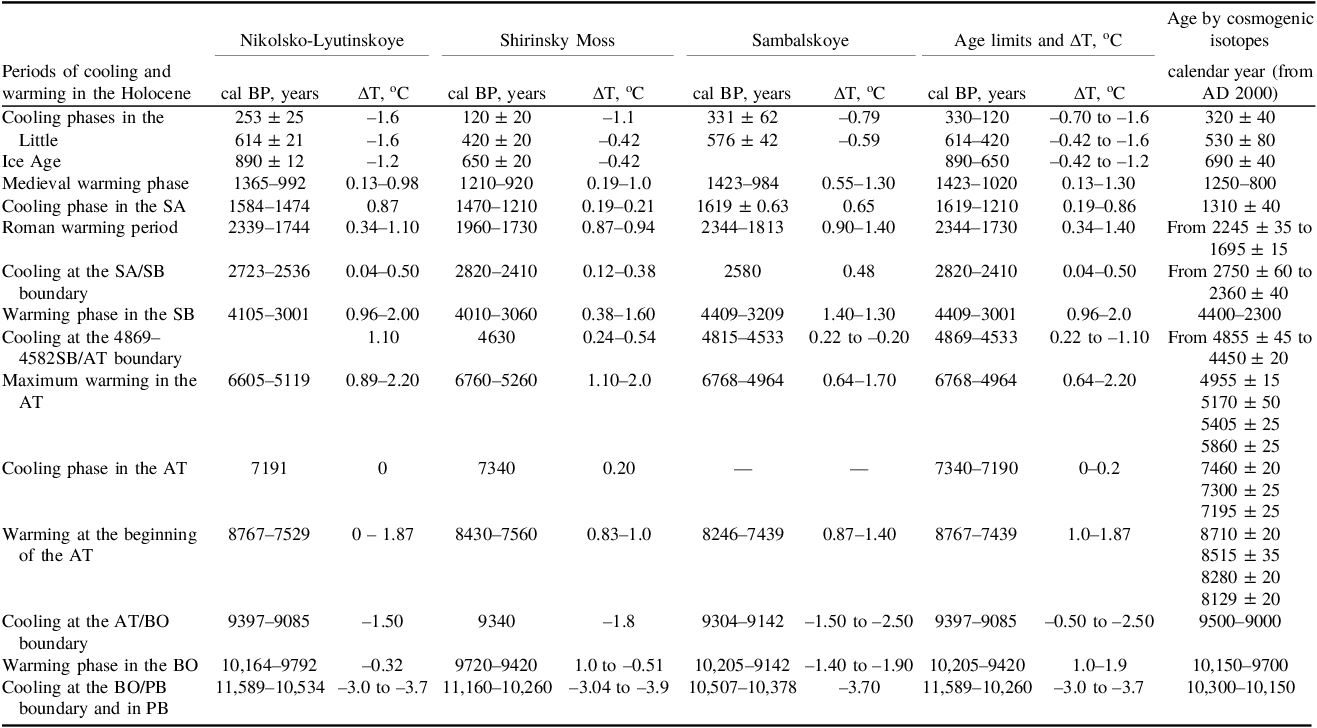
In Tables S1–S3 (see Supplement) 14C dates, calibrated intervals, and corrected ages for all the studied bogs, as well as the corresponding ΔT values, are presented. The ΔTs for the studied sections on a single scale of the calibrated age are shown in Figure 2. Table 1 shows the intervals of the corrected ages for cooling and warming stages and the corresponding ΔT values.
Reconstruction of ΔT for a period of 200–11,000 cal BP based on the analysis of sediments from the Nikolsko-Lyutinskoye (a), Shirinsky Mokh (b), and Sambalskoye (c) bogs.

Chronology of the stages of cooling and warming in the Holocene in Northwest Russia based on the analysis of deposits of the Nikolsko-Lyutinskoye, Shirinsky Moss, and Sambalskoye bogs, and the corresponding chronology based on the content of cosmogenic isotopes 14C and 10Be. The numerical values of the modeled age of peat samples and deviations in average annual temperature (ΔT) are from the data in Tables S1–S3. The designations SA, SB, AT, BO, PB represent the Subatlantic, Subboreal, Atlantic, Boreal, and Preboreal periods of the Holocene, respectively.

Table 1. Long description
The table presents data on cooling and warming phases in the Holocene across three bogs: Nikolsko-Lyutinskoye, Shirinsky Moss, and Sambalskoye. It includes periods of cooling and warming, with corresponding calendar years BP, temperature changes (ΔT in °C), and age limits. The table has 12 rows and 12 columns. Column headers include periods of cooling and warming, calendar years BP, ΔT in °C for each bog, age limits, and age by cosmogenic isotopes. Row labels include specific phases like the Little Ice Age, Medieval warming phase, and Roman warming period. Notable trends include varying temperature changes across different periods and bogs, with specific calendar years and age limits provided for each phase.
When correlating the age and ΔT values for samples from these sections (Tables S1–S3), it is necessary to take into account the errors in determining these quantities. Most of the dates were determined with a statistical error of up to 100 years, but several samples were dated with an error of up to 140–250 years. In parts of the calibration curve where oscillations in the 14C concentration are observed due to short-term 14C variations in the atmosphere, the calibrated age is determined using calibration programs in a wider age range. The calibrated age of majority of dated samples agrees with the corrected age within the dating error. However, the calibrated age of some samples is slightly underestimated compared to the calibrated age, which is probably due to the penetration of rootlets and rhizomes of younger plants into the 14C-dated samples.
A noticeable dating error can be caused by the penetration of roots and rhizomes of marsh plants, such as cotton grass and shrubs, into the underlying layers, which leads to age inversion in the peat bog section (samples LU-3481 and LU-3489 for Nikolsko-Lyutinskoye bog, Table S1; and samples LU-3183 and LU-3196 for Sambalskoye bog, Table S3). Therefore, the model allowed us to record contamination of the samples with younger or older carbon. The samples with inverted age were excluded from further analysis.
The accuracy of dating and determining the ΔT values depends significantly on the rate of peat accumulation. In the Nikolsko-Lyutinskoye section, peat at a depth of 50–250 cm accumulated at a rate of 0.83 mm/year; at a depth of 250–310 and 470–600 cm – 0.28 and 0.30 mm/year, respectively; and at a depth of 310–470 cm – 0.48 mm/year (Table S1). At the indicated rates of peat accumulation, 10 cm thick layers of peat were formed over 120, 357 and 208 calendar years, respectively. A decrease in the peat accumulation rate was also revealed in the deposits of the Shirinsky Mokh (0.33 mm/year) at a depth of 200–340 cm, and the Sambalskoye (0.29 mm/year) at a depth of 517–587 cm, which were formed at ca. 7340–3060 and 9142–6945 cal BP, respectively (Tables S2–S3). With a peat accumulation rate of 0.29 mm/year, the 10 cm thick layer was formed over 345 years, and the ΔT value is a smoothed average for such a long time interval.
Differences in the amplitude of ΔT changes are largely due to the error equal to ± 0.6 °C (Arslanov et al. Reference Arslanov, Savelyeva, Gey, Klimanov, Chernov, Chernova, Kuzmin, Tertychnaya, Subetto and Denisenkov1999; Klimanov Reference Klimanov and Velichko1994); the latitude and longitude of the studied section; possibly, local environmental conditions; and the accuracy of determining the age of the cooling and warming stages.
In the three sections of bog deposits under consideration, cooling and warming stages were identified (Table 1; Figure 2). The corrected ages for the coolings and warmings in most cases agree with each other within an error of 200–250 years.
In the studied sections, the lowest ΔT values were identified in the Little Ice Age (LIA) dated to ca. 120–890 cal BP. In the deposits of the Nikolsko-Lyutinskoye bog, the cooling phases in the LIA were determined (Tables 1, S1–S3). Taking into account the above sources of dating errors, these cooling phases can be correlated with the well-established Maunder (AD 1645–1714), Spörer (AD 1416–1534), and Wolf (AD 1282–1342) minima of solar activity, corresponding to the coldest phases of the LIA (Stuiver and Quay Reference Stuiver and Quay1980). During the LIA coolings, the average annual temperature was ca. 1.0–1.6 °C lower than the modern one (Table 1). Throughout the Medieval warming period at ca. 1223–920 cal BP, the average annual temperature exceeded the modern one by 0.13–1.3 °C. During the preceding cooling stage at ca. 1619–1210 cal BP, the average annual temperature decreased to 0.19 to –0.87 °C. In the interval of ca. 2344–1730 cal BP, the average annual temperature increased by 0.34–1.4 °C compared to the modern value (Roman warm period). At the turn of the Subatlantic/Subboreal periods, ca. 2800–2400 cal BP, the ΔT value decreased to 0.19 to –0.87 °C. During the warming in the Subboreal period, ca. 4400–3000 cal BP, ΔT was ca. 1.0–2.0 °C. According to the study of the Nikolsko-Lyutinskoye sediments in the interval of ca. 3675–3317 cal BP, the ΔT value decreased from 1.9 to 0.14 (Table 1). During the cooling at the boundary of the Subboreal/Atlantic periods at ca. 4869–4533 cal BP, ΔT decreased to –0.2 to –1.1°C.
In the Atlantic period, two warming stages are distinguished. The maximum warming occurred at ca. 6368–4960 cal BP when the average annual temperature was 0.6–2.2 °C higher than the current value. In the Nikolsko-Lyutinskoye deposits, cooling phases were identified at ca. 5365 ± 34 and ca. 6006 ± 48 cal BP (Table 1). At ca. 7340–7200 cal BP, there was a short-term cooling, and the average annual temperature decreased to the current level (ΔT = 0.0–0.2 °C). In the first half of the Atlantic period, ca. 8770–7440 cal BP, the ΔT was within the range of 1–1.9 °C.
During the cooling at the boundary of the Atlantic/Boreal periods, ca. 9400–9085 cal BP, the ΔT decreased to a value of –1.5 to –2.5 °C. During the warming in the Boreal period, ca. 10,200–9400 cal BP, the ΔT reached a value of 1.0 to –0.3 °C near the Nikolsko-Lyutinskoye and Shirinsky Mokh bogs, and –1.4 to –1.9 °C near the Sambalskoye bog. During the cooling at the boundary of the Boreal/Preboreal periods and the Preboreal period ca. 11,000–10,300 cal BP, the ΔT was –3.4 to –4.5 °C.
The data presented in Table 1 indicate that the cooling and warming stages within the above-mentioned dating errors occurred simultaneously in the studied bog sediments located in the northern, central, and southern parts of northwestern Russia. This is similar to the results of the study the pollen-and-spore data for Western and Central Europe (e.g., Davis et al. Reference Davis, Brewer, Stevenson, Guiot and Contributors2003). The synchronicity of changes in the average annual temperature is more clearly expressed in deposits formed at a rate of more than 0.4–0.5 mm/year, and it is less clear in the areas where peat accumulated at a lower rate.
3.2. Correlation of the chronology for short-term climate changes in northwestern Russia with data from other regions
It is of interest to compare the results of our reconstruction with data for other regions. Klimanov (Reference Klimanov and Velichko1994), using the information-statistical method which he developed for determining the average annual, July, and January temperatures, and the average annual precipitation for numerous sections of lake and bog deposits (in total, more than 60), constructed quantitative paleotemperature curves for the Holocene. The studied sections extend from the northwestern and central regions of the Russian Plain to the Russian Far East. The most noticeable extremes of cooling were identified at ca. 10,700, 9200, 7300, 5100, 3300, 2600, 1800, 1400, 1160, 700, 530, 250, and 100 cal BP. These cooling peaks within the considered errors in age determination are generally consistent with our results (Table 1). According to Klimanov (Reference Klimanov and Velichko1994), the data obtained indicate that in the humid zone of Northern Eurasia temperature changes were simultaneous but had different amplitudes. In the northern regions, the range of temperature changes was greater than in the southern territories.
Velichko et al. (Reference Velichko, Andreev and Klimanov1997) studied the dynamics of climate and vegetation during the Late Glacial and the Holocene in latitudinal zones from 68° to 54° N from the northwestern to the far eastern regions of Russia. Based on the palynological data and using the information-statistical method by Klimanov (Reference Klimanov1976), quantitative parameters of the climate for the warming and cooling stages in the Holocene were determined. The extremes of the cooling phases were established at ca. 10,800, 9140, 7300, 5150, 2700, and 1400 cal BP. Warming intervals were determined at ca. 11,250 (Polovetsk event), 9500 (Boreal period optimum), 9000–7400 (early Atlantic period), 6850–5700 (Holocene climatic optimum), 3800 (Subboreal period optimum), 2000, and 950 (Medieval optimum) cal BP. The presented numerical data on the chronology of the warming and cooling stages basically agree, within the limits of dating error, with the data we obtained for northwestern Russia (Table 1).
E. Y. Novenko and co-authors traced changes in the Holocene vegetation and climate in the central regions of the Russian Plain. They studied in most detail the deposits of the Staroselsky Moss bog in the south of the Valdai Upland and the Klyukva bog in the Oka River basin (Novenko and Olchev Reference Novenko and Olchev2015; Novenko et al. Reference Novenko, Tsyganov, Pisarchuk, Volkova, Babeshko, Kozlov, Shilov, Payne, Mazei and Olchev2018). In order to reconstruct paleoclimates, they used the “best analogues method” (Novenko et al. Reference Novenko, Zyuganova and Olchev2014). According to their paleotemperature curves, cooling phases were identified at ca. 10,000, 9200–8900, 8100–7900, 4800, 4200, 3500, 2800, 1400, and 650–400 cal BP. In most cases, they are comparable with the numerical indicators of cooling phases in northwestern Russia (Table 1). The stages of warming in the Boreal (ca. 9800–9300 cal BP), Early Atlantic (8900–7500 cal BP), Late Atlantic (7000–5000 cal BP), Subboreal (4700–2900 cal BP), and Early Subatlantic (1200–800 cal BP) periods are also consistent with the stages of warming in northwestern Russia (Table 1).
Among the works devoted to the reconstruction of quantitative parameters of the Holocene climate, studies carried out in Finland, Sweden, Estonia, and Latvia also deserve attention. In Finland, sediments of Lake Laihalamni in the south of the country were studied; in southern Sweden – Lake Flarken; in Estonia – Lake Raigastvere; and in Latvia – Lake Karjanovo (Heikkila and Seppa Reference Heikkilä and Seppä2003; Seppa and Poska Reference Seppä and Poska2004; Seppa et al. Reference Seppä, Hammarlund and Antonsson2005; Heikkila and Seppa Reference Heikkilä and Seppä2010). According to these data, the average annual temperature increased in the Boreal period and reached its modern value at ca. 9000–8600 cal BP. In the interval of 8600–8100 cal BP, a cooling occurred and the temperature decreased by 0.5 °C (Heikkila and Seppa Reference Heikkilä and Seppä2003) to 1.5 °C (Seppa and Poska Reference Seppä and Poska2004; Seppa et al. Reference Seppä, Hammarlund and Antonsson2005). Seppa and Poska (Reference Seppä and Poska2004) and Heikkila and Seppa (Reference Heikkilä and Seppä2010) correlate this cooling with the well-known “8200 cal BP event” which was the transfer of cold glacial waters from dammed lakes of the Laurentide Ice Sheet into the Atlantic Ocean at ca. 8500 cal BP. This weakened the Atlantic meridional gyre and caused cooling in North America and northern Europe (Alley & Ágústsdóttir, Reference Alley and Ágústsdóttir2005).
The same mechanism of cold water inflow from melting glaciers and weakening of the thermohaline circulation in the Atlantic Ocean, according to Wanner et al. (Reference Wanner, Beer, Bütikofer, Crowley, Cubasch, Flückiger, Goosse, Grosjean, Joos, Kaplan, Küttel, Müller, Prentice, Solomina, Stocker, Tarasov, Wagner and Widmann2008), explains the cold climate in the Early Holocene in North America and northern Europe, although summer insolation during this period was high. It should be noted that at ca. 11,000–10,300 cal BP solar activity was also high (Usoskin et al. Reference Usoskin, Solanki and Kovaltsov2007, Fig. 3).
Large-scale temperature reconstructions for the period AD 1000–1979: 1 – from Mann et al. (Reference Mann, Bradley and Hughes1999); 2 – from Esper et al. (Reference Esper, Frank, Wilson and Briffa2005); 3 – from Moberg et al. (Reference Moberg, Sonechkin, Holmgren, Datsenko and Karlen2005).

Beginning at ca. 8100 cal BP, the annual temperature increased rapidly, and during ca. 8000–4500 cal BP the warmest phase of the Atlantic period—the Holocene climatic optimum—was observed. In Finland, the average annual temperature reached its maximum value in the interval of ca. 8000–5800 cal BP, exceeding the modern value by 1.5–2 °C (Heikkila and Seppa Reference Heikkilä and Seppä2003). During ca. 7000–6700 cal BP, a cooling phase was detected. In the southeastern regions of Estonia and Latvia at ca. 8000–4500 cal BP the maximal annual temperature was 2.5–3 °C higher than the modern value (Seppa and Poska Reference Seppä and Poska2004; Heikkila and Seppa Reference Heikkilä and Seppä2010). According to some scholars (Heikkila and Seppa Reference Heikkilä and Seppä2003, Reference Heikkilä and Seppä2010; Seppa and Poska Reference Seppä and Poska2004; Seppa et al. Reference Seppä, Hammarlund and Antonsson2005), from ca. 4500–4300 cal BP until the present time the average annual temperature has gradually decreased by 1.5 °C. The smoothed paleotemperature curves after ca. 4500 cal BP do not reflect the known cooling events at ca. 2800–2700 cal BP and the LIA, as well as the Roman and Medieval warming stages. Heikkila and Seppa (Reference Heikkilä and Seppä2003) noted that the age–depth model they use does not allow the accurate determination of short-term events in the climatic reconstructions of Northern Europe, and another high-resolution temperature reconstruction is needed. The proposed conclusions are based on a small number (6–13) of 14C dates, which complicates the correct dating of short-term climate changes.
In order to determine the cooling periods in the Middle–Late Holocene, Wanner et al. (Reference Wanner, Solomina, Grosjean, Ritz and Jetel2011) analyzed temperature change data from 46 sections of Holocene marine, lake, and bog sediments, and cave stalagmites, located mainly in the Northern Hemisphere. Based on their data, cooling periods were identified in the following time intervals: ca. 8600–8000, 6500–5900, 4800–4500, 3300–2500, and 1750–1350 cal BP, and AD 1250–1850. The authors noted that periods of low temperature often coincide with periods of low solar activity, but at the same time processes such as explosive eruptions of tropical volcanoes, fluctuations in the thermohaline circulation in the Atlantic Ocean, changes in the intensity of the monsoon system in the African-Pacific region and currents in the Arctic Basin, and anthropogenic changes (especially in the 20th–21st centuries), can play an important role in short-term climate changes.
The use of high-frequency dating and modeling methodology made it possible to identify and date three main cooling phases in the LIA. By taking into account the dating errors, the numerical values of short-period coolings established in the Holocene of northwestern Russia in most cases agree with the chronology of cooling stages presented in the works by Klimanov (Reference Klimanov and Velichko1994), Velichko at al. (1997), Khotinsky and Klimanov (Reference Khotinsky and Klimanov1997), Novenko et al. (Reference Novenko, Zyuganova and Olchev2014, Reference Novenko, Tsyganov, Pisarchuk, Volkova, Babeshko, Kozlov, Shilov, Payne, Mazei and Olchev2018), Novenko and Olchev (Reference Novenko and Olchev2015), and Wanner et al. (Reference Wanner, Solomina, Grosjean, Ritz and Jetel2011), as well as with the reconstruction of ambient temperature based on the analysis of the oxygen isotope composition in Greenland ice cores (Alley Reference Alley2000; Wanner et al. Reference Wanner, Solomina, Grosjean, Ritz and Jetel2011).
3.3. Correlation of cooling stages and periods of mountain glacier advances
Advances and retreats of mountain glaciers are closely related to changes in air temperature and precipitation. At high and middle latitudes, stages of glacier advances correlate with multi-decadal periods of decreasing summer temperatures (Wanner et al. Reference Wanner, Beer, Bütikofer, Crowley, Cubasch, Flückiger, Goosse, Grosjean, Joos, Kaplan, Küttel, Müller, Prentice, Solomina, Stocker, Tarasov, Wagner and Widmann2008). The dynamics of mountain glaciers have been studied in detail in the Swiss Alps. The largest glaciers—the Great Aletch, Gorner, and Lower Grindelwald—advanced synchronously at ca. 3000–2600 BC, 500–600 BC, 800–900 BC, 1100–1200 BC, and 1300–1500 BC, and in the LIA at ca. AD 1300–1385, AD 1600–1667, and AD 1820–1860 (Holzhaser et al. Reference Holzhauser, Magny and Zumbühl2005).
According to Wanner et al. (Reference Wanner, Beer, Bütikofer, Crowley, Cubasch, Flückiger, Goosse, Grosjean, Joos, Kaplan, Küttel, Müller, Prentice, Solomina, Stocker, Tarasov, Wagner and Widmann2008), in several parts of the world mountain glaciers advanced more or less simultaneously at ca. 5400–4800, 3800, 3100, and 2500 cal BP. Over the past 2000 years, glaciations occurred in AD 600 and AD 1050–1150, and 2–3 major glacier advances occurred between AD 1300 and AD 1850. In the Alps, Alaska, and the Rocky Mountains, glaciers reached their maximum in AD 1300, AD 1450, AD 1650, and AD 1850, which are generally synchronous with the Wolf, Spörer, Maunder, and Dalton solar minima, respectively (Wanner et al. Reference Wanner, Beer, Bütikofer, Crowley, Cubasch, Flückiger, Goosse, Grosjean, Joos, Kaplan, Küttel, Müller, Prentice, Solomina, Stocker, Tarasov, Wagner and Widmann2008). A similar chronology of glacier advances has been established in the Altai Mountains of Siberia where a large number of tree trunk fragments were buried by glaciers that advanced in the range of AD 1200–1800. Tree trunk dates established by dendrochronological methods correspond to the intervals of AD 1250–1260, 1320–1380, 1440–1510, and 1640–1740 (Agatova et al. Reference Agatova, Nazarov, Nepop and Rodnight2012; Solomina et al. Reference Solomina, Bradley, Jomelli, Geirsdottir, Kaufman, Koch, McKay, Masiokas, Miller, Nesje, Nicolussi, Owen, Putnam, Wanner, Wiles and Yang2016). These intervals of glacier advances are in good agreement with the chronology of the listed solar activity minima.
Holzhaser et al. (Reference Holzhauser, Magny and Zumbühl2005) compared the fluctuations of the Great Aletsch glacier with variations in the 14C concentration in the atmosphere over the past 3500 years. They found a close correlation between the following parameters: periods of maximum glacier expansion corresponded to the highest 14C concentrations, and, conversely, minimum glacier expansion corresponded to lowest 14C concentrations. The presence of such a pattern, according to Holzhaser et al. (Reference Holzhauser, Magny and Zumbühl2005), supports the hypothesis that solar activity variations are the main factor in the formation of climate in the western part of Central Europe in the Late Holocene. They also established a correlation between the periods of the Great Aletsch glacier advance and periods of high levels in 20 lakes on the Swiss Plateau, the Jura Mountains, and the foothills of the Alps in northern France. According to the results obtained, higher lake levels were observed during 800–400 BC, AD 650–850, AD 1050–1250, and AD 1300–1860 (Wanner et al. Reference Wanner, Solomina, Grosjean, Ritz and Jetel2011). The last period of high lake levels consists of three phases, which are generally synchronous with the stages of glacier advances during the Wolf and Maunder solar minima.
A comparison of the information on the chronology of the advances of large mountain glaciers in a number of locations in the Northern Hemisphere with our data for northwestern Russia (Table 2) generally indicates the synchronicity of the stages of mountain glacier advances and the periods of cooling. The synchronicity of these events suggests a single external factor that caused these phenomena, which could be a decrease in total solar radiation and solar activity.
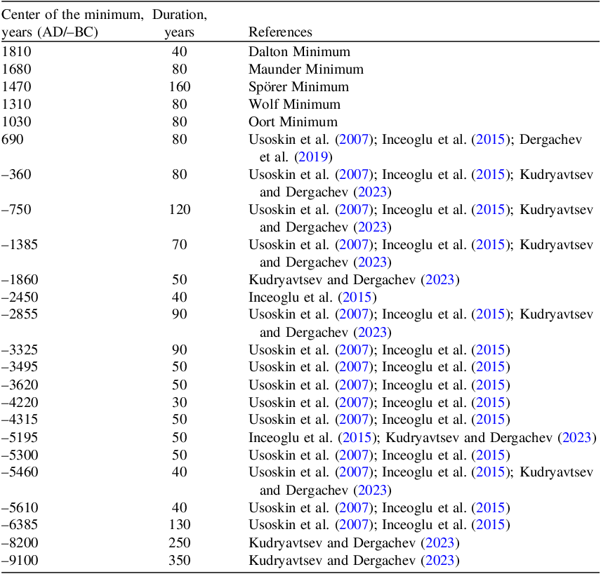
Centers of the grand minima of solar activity in the Holocene and their duration.

Table 2. Long description
A table with 19 rows and 3 columns. The columns are labeled ‘Center of the minimum, years (AD/–BC)’, ‘Duration, years’, and ‘References’. The table lists various periods of solar activity minima, their durations, and references. Row 1: 1810, 40, Dalton Minimum. Row 2: 1680, 80, Maunder Minimum. Row 3: 1470, 160, Spörer Minimum. Row 4: 1310, 80, Wolf Minimum. Row 5: 1030, 80, Oort Minimum. Row 6: 690, 80, Usoskin et al. (2007); Inceoglu et al. (2015); Dergachev et al. (2019). Row 7: -360, 80, Usoskin et al. (2007); Inceoglu et al. (2015); Kudryavtsev and Dergachev (2023). Row 8: -750, 120, Usoskin et al. (2007); Inceoglu et al. (2015); Kudryavtsev and Dergachev (2023). Row 9: -1385, 70, Usoskin et al. (2007); Inceoglu et al. (2015); Kudryavtsev and Dergachev (2023). Row 10: AQ60, 50, Kudryavtsev and Dergachev (2023). Row 11: -2450, 40, Inceoglu et al. (2015). Row 12: -2855, 90, Usoskin et al. (2007); Inceoglu et al. (2015); Kudryavtsev and Dergachev (2023). Row 13: -3325, 90, Usoskin et al. (2007); Inceoglu et al. (2015). Row 14: -3495, 50, Usoskin et al. (2007); Inceoglu et al. (2015). Row 15: -3620, 50, Usoskin et al. (2007); Inceoglu et al. (2015). Row 16: -4220, 30, Usoskin et al. (2007); Inceoglu et al. (2015). Row 17: -4315, 50, Usoskin et al. (2007); Inceoglu et al. (2015). Row 18: -5195, 50, Inceoglu et al. (2015); Kudryavtsev and Dergachev (2023). Row 19: -5300, 50, Usoskin et al. (2007); Inceoglu et al. (2015). Row 20: -5460, 40, Usoskin et al. (2007); Inceoglu et al. (2015); Kudryavtsev and Dergachev (2023). Row 21: -5610, 40, Usoskin et al. (2007); Inceoglu et al. (2015). Row 22: -6385, 130, Usoskin et al. (2007); Inceoglu et al. (2015). Row 23: -8200, 250, Kudryavtsev and Dergachev (2023). Row 24: -9100, 350, Kudryavtsev and Dergachev (2023).
4. Discussion
4.1. Correlation of variation in solar activity and the content of cosmogenic isotopes 14C and 10Be in the atmosphere and natural archives
Regular observations of solar activity, quantitatively expressed by the numbers of sunspots (Wolf numbers), have been conducted since the invention of the telescope in AD 1610. Detailed studies of changes in the parameters of total solar radiation, solar activity, solar magnetic field, intensity of galactic cosmic rays, and the rate of formation of cosmogenic isotopes 14C and 10Be show a close relationship between these values. For example, changes in the rate of the formation of 10Be during three 11-year solar cycles (AD 1975–2010) showed a directly proportional relationship between the total solar radiation, solar activity, and the solar magnetic field, and an inversely proportional relationship between the listed parameters and the intensity of galactic cosmic rays and the rate of formation of the 10Be isotope (Gray et al. Reference Gray, Beer, Geller, Haigh, Lockwood, Matthes, Cubasch, Fleitmann, Harrison, Hood, Luterbacher, Meehl, Shindell, van Geel and White2010).
The results of studies of variations in the listed parameters over the past 400 years, covering the period of instrumental determinations of sunspot numbers, demonstrate the synchronous increase in total solar radiation, solar activity, and the screening effect of the solar magnetic field. This leads to a decrease in the flux of galactic cosmic rays and the rate of formation of 14C and 10Be. Conversely, with a decrease in the intensity of solar radiation, solar activity, and the solar magnetic field, the rate of formation of cosmogenic isotopes raised.
The 14C and 10Be isotopes are formed in the upper atmosphere by the interaction of galactic cosmic ray nuclei with atmospheric gas atoms. Radiocarbon is oxidized to CO2 shortly after its formation and within less than 10 years mixes with atmospheric CO2 and carbonates dissolved in the surface water (upper 75 m) of the oceans, which together contain about 1360 billion tons of carbon (Arslanov Reference Arslanov1987). The CO2 gas is assimilated by plants and living organisms through photosynthesis and biological absorption. Measurements of 14C concentration in the annual tree rings collected from many points in the Northern Hemisphere showed the same (within an error of 0.5%) concentration of 14C. After formation in the atmosphere, 10Be is absorbed on aerosols, after which it falls to the Earth’s surface as part of atmospheric precipitation, including glaciers and marine sediments.
By measuring the 14C activity in tree rings, data were obtained of the change in 14C concentration covering the Holocene (Stuiver and Quay Reference Stuiver and Quay1980; Stuiver et al. Reference Stuiver, Reimer, Bard, Beck, Burr, Hughen, Kromer, McCormac, van der Plicht and Spurk1998). In the last millennium, the maximа in the relative concentration of 14C (Δ14C) were repeated approximately every 200 years, and corresponded to the solar activity minima—Maunder, Spörer, and Wolf. Long-term (thousands of years) and short-term (hundreds of years) Δ14C fluctuations in tree rings are distinguished. It is necessary to note that the intervals of increased amplitudes of 14C concentration, which occurred at ca. 9500, 7200, 5400, 2700, 500 cal BP are repeated approximately every 2400 years. The data indicate that there is a proportional relationship between solar activity and the concentration of 14C and 10Be in natural archives.
Reconstructions of solar activity, based on measurements of 10Be in the GRIP Greenland ice core and 14C in tree rings, showed identical synchronous changes in minima and maxima of solar activity (Wanner et al. Reference Wanner, Beer, Bütikofer, Crowley, Cubasch, Flückiger, Goosse, Grosjean, Joos, Kaplan, Küttel, Müller, Prentice, Solomina, Stocker, Tarasov, Wagner and Widmann2008; Vonmoos et al. Reference Vonmoos, Beer and Muscheler2006; Müller et al., Reference Müller, Joos, Edwards and Stocker2006). The measured values of 14C refer to the precisely established calendar age of tree rings. In view of this, the reconstruction of solar activity beyond instrumental measurements of sunspot numbers using cosmogenic isotopes is, in the opinion of most researchers, one of the main methods for reconstructing solar activity (e.g., Gray et al. Reference Gray, Beer, Geller, Haigh, Lockwood, Matthes, Cubasch, Fleitmann, Harrison, Hood, Luterbacher, Meehl, Shindell, van Geel and White2010; Wanner et al. Reference Wanner, Beer, Bütikofer, Crowley, Cubasch, Flückiger, Goosse, Grosjean, Joos, Kaplan, Küttel, Müller, Prentice, Solomina, Stocker, Tarasov, Wagner and Widmann2008, Reference Wanner, Solomina, Grosjean, Ritz and Jetel2011).
In Wanner et al. (Reference Wanner, Solomina, Grosjean, Ritz and Jetel2011, Fig. 1, a), reconstructions of air temperature, based on the analysis of the 18O isotope composition in the GISP-2 Greenland ice core over the past 10,000 years, are shown. This reconstruction shows that in the Holocene low temperatures were observed at ca. 700–250, 1580–1100, 3000–2600, 4000–3800, 4900–4400, 6700–6300, 7300–7100, and 8500–8100 cal BP; and warming stages at ca. 1100–800, 2300–1900, 3500–3100, 4300–4150, 5300–5000, 5800–5600, 7000–6800, 7900–7500, and 9200–8700 cal BP.
The reconstructions of solar activity over the past 6000 years based on the 10Be and 14C are shown in Wanner et al. (Reference Wanner, Beer, Bütikofer, Crowley, Cubasch, Flückiger, Goosse, Grosjean, Joos, Kaplan, Küttel, Müller, Prentice, Solomina, Stocker, Tarasov, Wagner and Widmann2008, Fig. 7). According to them, low values of solar activity over the past 6000 years were identified at ca. 700–250, 1400–1150, 2800–2650, 4500–4300, 5000–4750, and 5650–5400 cal BP. Stages of high solar activity were determined at ca. 150–0, 1150–700, 1800–1400, 2200–2000, 2650–2450, 3050–2850, 4300–3500, 4750–4550, 5150–4950, and 6000–5650 cal BP. The extremes of the grand minima of solar activity are established at ca. 500, 1320–1260, 2300, 2700, 3350, 4450, 4880, 5230, and 5580 cal BP. These numerical indicators are practically identical to the centers of the main minima of solar activity given in Table 3. Thus, a comparative analysis of the chronology for the cooling phases and extremes of the main minima of solar activity generally indicates a synchronous correlation between changes in ambient temperature and solar activity.
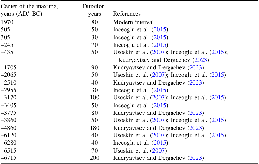
Centers of the grand maxima of solar activity in the Holocene and their duration.

Table 3. Long description
A table with three columns and thirteen rows. The columns are labeled ‘Center of the maxima, years (AD/–BC)’, ‘Duration, years’, and ‘References’. The table lists specific years marking the center of solar activity maxima, the duration of these maxima in years, and references to studies that support these data points. The years range from 6715 BC to 1970 AD, with durations varying from 30 to 200 years. The references include studies by Usoskin et al., Inceoglu et al., and Kudryavtsev and Dergachev, among others.
4.2. Correlation of changes in 14C and 10Be isotopes from natural archives and short-term climate changes
From historical chronicles and studies of climate changes, two periods of extreme climate and solar activity have been established over the past millennium: the Little Ice Age (ca. AD 1300–1850) and the Warm Medieval Period (ca. AD 900–1300), which have a global manifestation (e.g., La Roy Ladurie Reference Le Roy Ladurie1967).
Figure 3 shows reconstructions of the air temperature in the Northern Hemisphere for the last 1000 years (Mann et al. Reference Mann, Bradley and Hughes1999) and the global temperature for the same period (Esper et al. Reference Esper, Frank, Wilson and Briffa2005). Synchronicity of temperature changes is observed in both reconstructions, but the temperature amplitudes often differ significantly. It clearly demonstrates low temperatures during the Maunder (AD 1645–1714), Spörer (AD 1416–1534), and Wolf (AD 1282–1342) solar activity minima, and higher air temperatures during the Medieval Warm Period (AD 800–1200) corresponding to higher solar activity. Tables 2–3 indicate the duration of episodes of high and low solar activity based on the 14C and 10Be contents.
Therefore, the confinement of the stages of mountain glacier advances to the time intervals of the Maunder, Spörer, and Wolf solar minima is clear, which are the coldest phases in the last millennium (Mann et al. Reference Mann, Bradley and Hughes1999; Esper et al. Reference Esper, Frank, Wilson and Briffa2005). The correspondence of the known major (grand) minimum of solar activity at ca. 2700 cal BP to the stage of cooling on the Subatlantic/Subboreal boundary (Wanner et al. Reference Wanner, Beer, Bütikofer, Crowley, Cubasch, Flückiger, Goosse, Grosjean, Joos, Kaplan, Küttel, Müller, Prentice, Solomina, Stocker, Tarasov, Wagner and Widmann2008) indicate a close relationship between changes in solar activity and short-term changes in ambient temperature. This point of view is shared by many researchers (e.g., Dergachev Reference Dergachev2017; Gray et al. Reference Gray, Beer, Geller, Haigh, Lockwood, Matthes, Cubasch, Fleitmann, Harrison, Hood, Luterbacher, Meehl, Shindell, van Geel and White2010; Mauquoy et al., Reference Mauquoy, van Geel, Blaauw and van der Plicht2002; Solomina et al. Reference Solomina, Bradley, Jomelli, Geirsdottir, Kaufman, Koch, McKay, Masiokas, Miller, Nesje, Nicolussi, Owen, Putnam, Wanner, Wiles and Yang2016; Wanner et al. Reference Wanner, Beer, Bütikofer, Crowley, Cubasch, Flückiger, Goosse, Grosjean, Joos, Kaplan, Küttel, Müller, Prentice, Solomina, Stocker, Tarasov, Wagner and Widmann2008). The use of the methodology by Wanner et al. (Reference Wanner, Beer, Bütikofer, Crowley, Cubasch, Flückiger, Goosse, Grosjean, Joos, Kaplan, Küttel, Müller, Prentice, Solomina, Stocker, Tarasov, Wagner and Widmann2008) of high-frequency dating and subsequent modeling made it possible to establish the chronology of short-term changes in air temperature and to compare the short-period cooling intervals in the Holocene of northwestern Russia (Table 1) with the chronology of solar activity minima (Table 2). From the data in Table 1, it follows that in most cases a correlation is observed between the chronology of cooling phases and solar activity minima throughout the Holocene, but the clearest correspondence is detected for the past several thousand years.
The good correlation of our approach to previously obtained results can be illustrated using the conclusions by Arslanov et al. (Reference Arslanov, Novenko, Sapelko, Dergachev, Nosevich, Maksimov, Petrov, Grigoriev, Denisenkov, Levchenko, Bolikhovskaya, Klyuvitkina and Yanina2020) who conducted a more detailed study of the sediments in the Shirinskoye Bog Nature Reserve in 2018. Sampling was carried out for 4-cm peat layers to a depth of 250 cm. Based on the 14C dates obtained and using the C. Bronk Ramsey’s model, the corrected (“modeled”) age of each 4-cm peat layer was determined from the modern period (AD 1950, depth 42–44 cm) to 2281 ± 22 BP (depth 246–250 cm). Using the “best analog method”, E.Yu. Novenko constructed the paleoclimatic curve (Arslanov et al. Reference Arslanov, Novenko, Sapelko, Dergachev, Nosevich, Maksimov, Petrov, Grigoriev, Denisenkov, Levchenko, Bolikhovskaya, Klyuvitkina and Yanina2020). This curve clearly shows the Roman warming in the range of ca. 1600–2200 cal BP, which was accompanied by the spread of coniferous-broadleaf forests.
During the subsequent cooling (1250–1600 cal BP), broadleaf forests disappeared and open spaces with grass cover increased. During the Medieval warm period (ca. 700–1250 cal BP), coniferous-broadleaf forests spread again. In the Little Ice Age, ca. 100–700 cal BP, 4 cooling phases were identified that correspond to the corrected ages of 63 ± 26, 311 ± 12, 344 ± 12, 408 ± 14, 530 ±14, and 675 ± 16 cal BP. At the cooling extremes, the average annual temperature was 1–1.8 ºC lower than the modern value. The identified cooling extremes turned out to be synchronous with the periods of minimum solar activity of Dalton, Maunder, Spörer, and Wolf (Table 3). The above values of the calibrated age of the warming and cooling stages in the Sherinskoye Bog section are in good agreement with the corrected age of the cold and warm stages in the Shirinsky Mokh section in Tables 1 and S2. The agreement of the results indicates the reliability of the methods of paleoclimate reconstruction, palynological analysis, dating, and age correction by modeling used in Arslanov et al. (Reference Arslanov, Novenko, Sapelko, Dergachev, Nosevich, Maksimov, Petrov, Grigoriev, Denisenkov, Levchenko, Bolikhovskaya, Klyuvitkina and Yanina2020).
To increase further the accuracy of dating short-term climate changes and to compare its chronology with solar activity, it is necessary to increase the frequency of 14C dates per section and continue palynological studies of lake and bog deposits. This could be useful to clarify certain issues related to the ongoing discussion about the role of Sun in climate changes (e.g., Scafetta Reference Scafetta2023; van Geel and Ziegler Reference van Geel and Ziegler2013).
5. Conclusions
Using the modeling methodology proposed by C. Bronk Ramsey, the corrected age of samples collected from raised bog sediments in northwestern Russia was determined, and a refined chronology of short-term climate changes in the Holocene was established. Based on the results obtained, a chronology of changes in vegetation and climate for northwestern Russia in the Late Glacial and Holocene was established, which includes a series of short-term warming and cooling stages lasting several hundred years. The quantitative climate parameters for warming and cooling stages in the Late Glacial and in the Holocene were obtained.
The short-period changes of mean annual temperature occurred mainly synchronously in the three studied sections of bog sediments. Changes in mean annual temperature were also mainly simultaneous with the chronology of temperature changes in the Northern Hemisphere over the past 1000 years and with the chronology established on the basis of the study of the GISP-2 Greenland ice core, as well as the chronology of mountain glacier advances.
Comparison of the chronology for the cooling and warming stages in the Holocene in northwestern Russia and the ages of the corresponding stages of low and high solar activity generally demonstrates the synchronicity of the stages of cooling with the periods of low solar activity, and the stages of warming with the periods of high solar activity. An illustrative example is the synchronicity of the stages of cooling during the periods of solar activity minima (Maunder, Spörer, Wolf, and Oort) in the last millennium, and in earlier periods, ca. 1300–1200, 2800–2300, 4850–4450, 7400–7200, and 9600–9000 cal BP. The established synchronicity of short-term climate changes and solar activity indicates that variations in solar activity are one of the main natural causes of short-period climate changes in the Holocene. This is an additional confirmation of the previously made conclusions about the important role of solar activity for short-term climate changes in the Holocene. Other forcing mechanisms, such as volcanic activity and shifts in oceanic circulation, also may be factors of short-term climate changes.
Supplementary material
To view supplementary material for this article, please visit https://doi.org/10.1017/RDC.2026.10268
Acknowledgments
The data used in this work were supported by a grant of the Russian Foundation for Basic Research (project No. 18-05-00381). The work by I.V. Kudryavtsev is in accordance with the state assignment of the Ioffe Institute No. FFUG-2024-0002.The final preparation of this paper was conducted with the help of the State Assignment of the Institute of Geology and Mineralogy SB RAS No. FWZN-2026-0004, with funding provided by the Ministry of Science and Higher Education of Russian Federation. We are grateful to Editor, Prof. A.J.T. Jull, for help with generating the P_Sequence modeling of 14C data for the Nikolsko-Lyutinskoye bog, and Associate Editor and anonymous reviewers for their useful comments.
Competing interests declaration
The authors do not have any competing interests.