


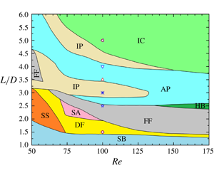


1 Introduction
Multiple cylindrical structures (e.g. heat exchanger tubes, marine riser bundles and undersea pipelines) are more frequently encountered in engineering practices than isolated ones, although less attention has been paid to the hydrodynamics of these multi-structure systems. While the flow around two cylinders has been investigated extensively, little attention has been paid to the flow around three circular cylinders. In this paper, the hydrodynamic forces, spectral features and wake structures of three cylinders in an equilateral configuration are investigated in a large parametric space to provide a thorough understanding of the underlying physics of fluid dynamics.
Due to the complexity of the problem, the flow past two circular cylinders is reviewed first. Zdravkovich (Reference Zdravkovich1977) classified the two-cylinder flow interference into proximity interference, wake interference and combined interference. For the flow around two tandem cylinders, three distinct flows (i.e. extended, reattachment and co-shedding) are observed based on the spacing ratio  $L/D$ (Zdravkovich Reference Zdravkovich1987; Alam et al. Reference Alam, Moriya, Takai and Sakamoto2003b; Papaioannou et al. Reference Papaioannou, Yue, Triantafyllou and Karniadakis2006; Sumner Reference Sumner2010; Alam Reference Alam2014), where
 $L$ is the centre-to-centre spacing of the cylinders and
 $D$ is the cylinder diameter. The extended-body flow appears at
 $L/D<1.2{-}1.8$ where the two cylinders are so close to each other that the free shear layers separating from the upstream cylinder overshoot the downstream one, and the flow in the cylinder gap is stagnant. In the reattachment case (
 $1.2{-}1.8<L/D<3.4{-}3.8$), the shear layers separating from the upstream cylinder reattach on the downstream cylinder and the flow in the gap is quasi-steady. The co-shedding flow materializes at
 $L/D>3.4{-}3.8$, where the shear layers roll up alternately in the gap between the cylinders and thus the flow in the gap is significantly unsteady. The
 $L/D$ separating the reattachment and co-shedding flows is known as the critical spacing. Note that the critical spacing is affected by many factors, such as the Reynolds number (
 $Re$), turbulence intensity of the incoming flow, etc. (Ljungkrona, Norberg & Sunden Reference Ljungkrona, Norberg and Sunden1991; Alam Reference Alam2014). A hysteresis behaviour was observed between the reattachment and co-shedding regimes for increasing and decreasing
 $L/D$ and
 $Re$ (Igarashi Reference Igarashi1981; Liu & Chen Reference Liu and Chen2002). In the transition from the reattachment to co-shedding patterns, the fluid forces and Strouhal (
 $St$) number jump from small to high values. Concomitantly, the mean drag coefficient leaps from a negative value to a positive value – termed the drag inversion (Carmo, Meneghini & Sherwin Reference Carmo, Meneghini and Sherwin2010). For all three regimes, the upstream cylinder significantly affects the flow around the downstream cylinder even at very large
 $L/D$. However, the effect of the downstream cylinder on the upstream one is only perceivable for
 $L/D<5.0$ (Papaioannou et al. Reference Papaioannou, Yue, Triantafyllou and Karniadakis2006).
For the side-by-side arrangement of two cylinders, the proximity interference occurs when the cylinders are close to each other. Five flow patterns were summarized in Sumner (Reference Sumner2010). When  $L/D$ is small (
 $L/D<1.1{-}1.2$), no gap flow exists between the cylinders and vortices are alternately shed from the free-stream sides of the cylinders (Alam, Moriya & Sakamoto Reference Alam, Moriya and Sakamoto2003a). The two cylinders behave like a single bluff body. For intermediate
 $L/D$ (
 $1.1{-}1.2<L/D<2.0{-}2.2$), the gap flow is weak, and two flow patterns, i.e. the deflected flow (DF) pattern and the flip-flopping (FF) pattern, intermittently appear. It is noted that the FF pattern shows clearly different characteristics between the low-
 $Re$ laminar flow and high-
 $Re$ turbulent flow. Kim & Durbin (Reference Kim and Durbin1988) (
 $Re=1.9\times 10^{3}{-}6.9\times 10^{3}$) found that the flip-over time interval of the gap flow is several orders of magnitude longer than the vortex-shedding period. On the other hand, for low-
 $Re$ flow (
 $Re=40{-}160$), the time scale is only a few vortex-shedding periods (Kang Reference Kang2003; Carini, Giannetti & Auteri Reference Carini, Giannetti and Auteri2014b). When
 $L/D$ is large (
 ${>}2.0{-}2.5$), in-phase or anti-phase flow patterns appear depending upon
 $L/D$ (Williamson Reference Williamson1985). In these two patterns, the flow interference between the cylinders is weak. Kang (Reference Kang2003) numerically simulated the flow past two side-by-side cylinders at
 $Re=40{-}160$,
 $L/D=1.0{-}6.0$, and his results showed six distinct near-wake patterns: anti-phase, in-phase, flip-flopping, deflected, single bluff-body and steady. Liu et al. (Reference Liu, Ma, Sun and Yin2007), in their numerical study of flow past two side-by-side cylinders at
 $Re=18{-}100$, further classified the near wake into nine patterns, including four steady ones (single bluff body, separated double body, transition and biased) and five unsteady ones (single bluff body, biased quasi-steady, flip-flopping, in-phase and anti-phase). Supradeepan & Roy (Reference Supradeepan and Roy2014) numerically investigated the near-wake patterns behind two side-by-side cylinders at
 $Re=100$ and
 $L/D=1.1{-}8.0$. They found that there exist five flow regimes, namely single bluff-body periodic (
 $L/D=1.1{-}1.3$), aperiodic (
 $L/D=1.4{-}2.2$), transiting (
 $L/D=2.3{-}3.1$), anti-phase (
 $L/D=3.2{-}7.9$) and in-phase (
 $L/D>8.0$).
For staggered arrangements of the two cylinders, all three kinds of flow interference (proximity, wake and combined interference) can be observed based on the angle of attack  $\unicode[STIX]{x1D6FC}$ and
 $L/D$. Zdravkovich (Reference Zdravkovich1987) experimentally observed two flow regimes for the flow past two staggered cylinders at high Reynolds numbers, i.e. a gap flow regime where an attractive lift appears and a wake displacement regime where a repulsive lift occurs. Akbari & Price (Reference Akbari and Price2005) found five different flow regimes in their numerical simulations of the flow past two staggered circular cylinders at
 $Re=800$. They were named the base bleed (
 $L/D\leqslant 1.1$ and
 $\unicode[STIX]{x1D6FC}\geqslant 30^{\circ }$), shear layer reattachment (
 $1.1<L/D<2.0$ and
 $\unicode[STIX]{x1D6FC}<10^{\circ }$), vortex pairing and enveloping (
 $1.0\leqslant L/D\leqslant 2.0$ and
 $\unicode[STIX]{x1D6FC}\geqslant 30^{\circ }$), vortex impingement (
 $L/D\geqslant 3.0$ and
 $\unicode[STIX]{x1D6FC}\leqslant 10^{\circ }$) and complete vortex-shedding (
 $L/D\geqslant 2.5$ and
 $\unicode[STIX]{x1D6FC}\geqslant 30^{\circ }$) flow regimes, respectively. Alam & Sakamoto (Reference Alam and Sakamoto2005) experimentally investigated the flow past two staggered circular cylinders at
 $Re=5.5\times 10^{4}$. A number of discontinuities in the flow were observed when
 $\unicode[STIX]{x1D6FC}$ and/or
 $L/D$ were varied. Alam & Meyer (Reference Alam and Meyer2013) identified that two cylinders interact with each other in six different interaction mechanisms, depending on
 $\unicode[STIX]{x1D6FC}$ and
 $L/D$. These were termed boundary layer–cylinder interaction, shear layer or wake–cylinder interaction, shear layer–shear layer interaction, vortex–cylinder interaction, vortex–shear layer interaction, and vortex–vortex interaction. While the vortex–cylinder interaction resulted in a very high fluctuating drag, vortex–shear layer interaction engendered a high fluctuating lift. Tong, Cheng & Zhao (Reference Tong, Cheng and Zhao2015) provided detailed physics in the flow past two staggered circular cylinders through a set of direct numerical simulations with
 $Re=10^{3}$. They found a strong flow three-dimensionality in the gap between the cylinders.
The flow around three cylinders is more complex than that around two. Igarashi & Suzuki (Reference Igarashi and Suzuki1984) experimentally studied the characteristics of flow around three tandem cylinders with  $L/D=1.0{-}4.0$ and
 $Re=1.09\times 10^{4}{-}3.92\times 10^{4}$. On account of the dynamic effects of the upstream-cylinder shear layers on the downstream cylinders, six flow patterns and two bistable flow regions were identified. Harichandan & Roy (Reference Harichandan and Roy2010) numerically investigated the flow past three stationary tandem cylinders with
 $L/D=2.0$ and 5.0 at
 $Re=100$ and 200. Results showed that the downstream cylinder experiences large unsteady forces that can give rise to a wake-induced flutter if the downstream cylinder is free to vibrate.
Moreover, Kang (Reference Kang2004) numerically simulated laminar flow past three side-by-side cylinders at  $Re=100$ and found that the flow patterns can be summarized into five different kinds based on
 $L/D$. These are single bluff body (
 $L/D<1.3$), deflected (
 $L/D\approx 1.3$), flip-flopping (
 $1.3<L/D\leqslant 2.2$), in-phase (
 $L/D\approx 2.5$) and modulation (
 $L/D\geqslant 3.0$). For the modulation pattern, the vortex-shedding frequency of the central cylinder is slightly larger than that of a side cylinder, and the modulation period is long. Han, Zhou & Tu (Reference Han, Zhou and Tu2013) carried out numerical simulations of the flow past three side-by-side cylinders at
 $Re=40{-}160$ which produced eight flow patterns: single bluff body, deflected, flip-flopping, non-identical and identical steady patterns, anti-phase and in-phase patterns and a combined pattern (consisting of the in-phase and anti-phase patterns). In their low-
 $Re$ cases, asymmetric and symmetric steady patterns were observed. Specifically, when
 $L/D$ is small, vorticities in the gap shear layers are much lower than those in the free-stream shear layers. However, when
 $L/D$ is large enough, three cylinders behave as isolated cylinders, and the vorticity field and hydrodynamic forces are the same for the three cylinders.
Flow past four cylinders in square arrangements has also been investigated by several researchers. Sayers (Reference Sayers1990) showed in their wind tunnel experiments that, for  $L/D\geqslant 4.0$, the frequency of vortex shedding from each of the four cylinders is similar to that of an isolated cylinder. Esfahani & Vasel-Be-Hagh (Reference Esfahani and Vasel-Be-Hagh2010) numerically demonstrated that there are three different flow patterns in the range of
 $L/D=1.5{-}4.5$, i.e. stable shielding flow, wiggling shielding flow and vortex-shedding flow. The critical spacing ratios between them are
 $L/D=2.5$ and 3.5, respectively. Results of Lam, Li & So (Reference Lam, Li and So2003) showed three flow patterns at
 $Re=2.25\times 10^{4}{-}5.18\times 10^{4}$. Recently, Esfahani & Vasel-Be-Hagh (Reference Esfahani and Vasel-Be-Hagh2013) found that there exists a transition between the anti-phase and in-phase patterns within the range of
 $L/D=2.0{-}3.0$ at
 $Re=200$.
Yang et al. (Reference Yang, Yan, Wu, Tu and Luo2016) studied the flow past three circular cylinders in equilateral-triangular arrangements at  $Re=50{-}200$ from the viewpoint of vortex-shedding suppression. Their results showed that, at
 $\unicode[STIX]{x1D6FC}=0^{\circ }$ (one upstream cylinder and the other two side-by-side downstream), the vortex shedding from the upstream cylinder is suppressed for
 $Re=100{-}200$. However, when
 $\unicode[STIX]{x1D6FC}=60^{\circ }$ (two upstream cylinders in side-by-side and one downstream cylinder), the suppression occurs on the downstream cylinder at
 $Re\leqslant 175$. de Paula, Endres & Möller (Reference de Paula, Endres and Möller2013) experimentally identified the bistable phenomenon at
 $L/D=1.6$ and
 $\unicode[STIX]{x1D6FC}=0^{\circ }$. Zheng, Zhang & Lv (Reference Zheng, Zhang and Lv2016) numerically investigated the flow past three equidistantly arranged cylinders at
 $Re=100$ and 200 with
 $L/D=1.5{-}7.0$. The deflected pattern appears when
 $\unicode[STIX]{x1D6FC}=0^{\circ }$, which is consistent with the findings in Yang et al. (Reference Yang, Yan, Wu, Tu and Luo2016). Moreover, the deflected pattern shows a clear dependence on
 $Re$: it disappears at
 $L/D\geqslant 2.0$ when
 $Re=100$ and at
 $L/D\geqslant 3.0$ when
 $Re=200$. Bao, Zhou & Huang (Reference Bao, Zhou and Huang2010) numerically investigated the same problem for
 $L/D=1.5{-}5.0$,
 $\unicode[STIX]{x1D6FC}=0^{\circ }{-}60^{\circ }$ and
 $Re=100$. Five flow patterns were confirmed, i.e. single bluff body, deflected, flip-flopping, in-phase and anti-phase. Moreover, they found that the flow interference between the three cylinders plays an important role in the variation of lift frequency. At a high
 $Re=6.2\times 10^{4}$, Tatsuno, Amamoto & Ishi-i (Reference Tatsuno, Amamoto and Ishi-i1998) experimentally studied the flow interference between three cylinders at
 $\unicode[STIX]{x1D6FC}=0^{\circ }{-}60^{\circ }$,
 $L/D=1.39{-}6.93$. When
 $L/D$ is small (
 ${<}2.6$), the interference is strong, leading to an asymmetric wake. On the other hand, at
 $L/D\geqslant 3.5$, the flow interference is weak and the wake becomes symmetric. Bansal & Yarusevych (Reference Bansal and Yarusevych2017) found a bistable flow pattern at
 $\unicode[STIX]{x1D6FC}=0^{\circ }$,
 $L/D=1.35$ and
 $Re=2.1\times 10^{3}$, without the switching of the gap flow direction. The biased direction of the gap flow is dependent on the initial flow conditions. This is consistent with the results of Lam & Cheung (Reference Lam and Cheung1988) at
 $Re=2.1\times 10^{3}{-}3.5\times 10^{3}$, where the bistable pattern appears when
 $L/D\leqslant 2.29$ at
 $\unicode[STIX]{x1D6FC}=0^{\circ }$.
By comparing with the flow around a single or a pair of cylinders, the flow past three equilateral-triangular-arranged circular cylinders is not well-investigated. Researchers have only carried out studies on the flow past three equispaced cylinders within a narrow parametric space. A systematic study on the flow around three cylinders and its dependence on  $Re$ and
 $L/D$ is still missing. The main objectives of this investigation are to establish an overall and comprehensive understanding of this problem in a wider parametric space of
 $L/D=1.0{-}6.0$ and
 $Re=50{-}300$ with fine increments in both
 $L/D$ and
 $Re$, and to inspect the influences of the wake three-dimensionality by performing three-dimensional direct numerical simulations.
The remains of the paper are organized as follows. In § 2, the adopted numerical methodology and the validation cases are presented. Section 3 presents the effects of the spacing ratio on flow features and hydrodynamics. The wake pattern, the drag and lift forces and the spectral frequency are discussed. The key roles of the Reynolds number are further elucidated in § 4. Section 5 discusses the flow regime partition in the  $Re-L/D$ parametric space, while § 6 inspect the influences of the wake three-dimensionality. The main conclusions are summarized in § 7.
2 Numerical methodology and validation cases
The governing equations for the fluid flow are the incompressible Navier–Stokes equations. The two-step predictor–corrector procedure is adopted for the decoupling of the flow governing equations, and the resulting pressure Poisson equation is solved by using the biconjugate gradients stabilized method and the multi-grid method. The second-order Adams–Bashforth time marching scheme is employed to calculate a new velocity field.
The flow around the cylinders is simulated by using the immersed boundary (IB) method which was first introduced by Peskin (Reference Peskin1972) in the simulation of blood flow around the leaflet of a human heart. In the framework of the IB method, the flow governing equations are discretized on a fixed Cartesian grid, which generally does not conform to the geometry of the cylinders. As a result, the boundary conditions on the fluid–cylinder interface cannot be imposed directly. Instead, an extra body force is added into the momentum equation to take such interaction into account. One of the advantages of the IB method lies in its parameterized and fast implementation of a large number of cases with different geometric configurations, compared with conventional methods using body-conformal grids. For the sake of conciseness, details of the methodology are not presented here and readers are referred to our previous work (Ji, Munjiza & Williams Reference Ji, Munjiza and Williams2012; Chen et al. Reference Chen, Ji, Xu, Liu and Campbell2015b; Chen, Ji & Xu Reference Chen, Ji and Xu2019) for further information.
The arrangement of the cylinders in the computational domain is presented in figure 1, where Cylinders 1, 2 and 3 are arranged in an equilateral triangle with Cylinder 1 placed upstream and Cylinders 2 and 3 side-by-side downstream. The spacing between the centres of two cylinders is defined as  $L$ and is varied from 1.0 to 6.0. The computational domain is
 $200D\times 200D$. The centre of the computational domain coincides with the centre of the triangle formed by the cylinder centres (figure 1). The origin of the (
 $x$,
 $y$) coordinate system is also located at the centre of the triangle. The smallest normalized grid spacing is set to
 $\unicode[STIX]{x0394}x/D=\unicode[STIX]{x0394}y/D=1/64$ in a region of
 $8D\times 8D$ surrounding the cylinders. This grid resolution has been demonstrated to be sufficiently fine by Chen et al. (Reference Chen, Ji, Wang, Xu and Campbell2015a,Reference Chen, Ji, Xu, Liu and Campbellb, Reference Chen, Ji, Williams, Xu, Yang and Cui2018). A Dirichlet-type boundary condition is adopted at the inflow and a Neumann-type boundary condition is employed at the outflow. The top and bottom walls are set as free-slip boundaries. To capture the long-period flow pattern, the two-dimensional (2-D) simulations are carried out for a non-dimensional time
 $t^{\ast }=tU/D>5000$, after a statistically stable flow state has been reached, where
 $U$ is the free-stream flow velocity.
The computational domain and boundary conditions for the flow past three cylinders in an equilateral-triangular arrangement.

Comparison of flow past an isolated circular cylinder at  $Re=50{-}200$.

Comparison of flow past two side-by-side cylinders at  $L/D=2.5$ and
 $Re=100$.

Comparison of flow past three circular cylinders in an equilateral-triangular arrangement with  $L/D=3.0$ and
 $Re=100$.

Flow past three circular cylinders in an equilateral-triangular arrangement at  $L/D=3.0$ and
 $Re=100$ with different
 $\unicode[STIX]{x0394}tU/D$.

In this study, the numerical methodology is validated for an isolated cylinder at  $Re=50{-}200$ (table 1), two side-by-side cylinders at
 $L/D=2.5$ and
 $Re=100$ (table 2) and three cylinders in an equilateral-triangular arrangement at
 $L/D=3.0$ and
 $Re=100$ (table 3) where the time-mean drag coefficient
 $\overline{C}_{d}$, fluctuating root-mean-square (r.m.s.) lift coefficient
 $C_{l}^{\prime }$ and Strouhal number
 $St$ are presented and compared with those in the literature. In table 1, the maximum discrepancy between the results is marginal, confirming a reasonably high accuracy of the adopted numerical methodology for the range of
 $Re$ examined. The present results in table 2 agree well with those in Kang (Reference Kang2003) and Bao et al. (Reference Bao, Zhou and Tu2013) which have the same blockage ratio
 $B(=D/H=0.005)$, where
 $H$ is the transverse width of the computational domain. The largest discrepancy (
 ${\sim}11.5\,\%$) is observed for
 $C_{l}^{\prime }$ between the present and that of Lee et al. (Reference Lee, Ha, Yoon and Balachandar2009). This discrepancy is attributed to the large
 $B(=0.02)$ in Lee et al. (Reference Lee, Ha, Yoon and Balachandar2009). Finally, for the three cylinders, the present results with
 $B=0.005$ are in good agreement with those in Bao et al. (Reference Bao, Zhou and Huang2010) with
 $B=0.01$. However, significant discrepancies are observed between the present results and those of Zheng et al. (Reference Zheng, Zhang and Lv2016) where
 $B=0.045$ is much larger than that
 $(=0.005)$ in the present computation. It is found that the difference in the present results between
 $B=0.0025$ and 0.005 is negligible, confirming that
 $B=0.005$ is small enough for the computation of the three-cylinder flow. Even the total blockage ratio
 $B^{\prime }=3D/H=0.015$, considering the blocking effects of three cylinders, still satisfies the criterion
 $({\sim}0.01{-}0.02)$ suggested in Sen, Mittal & Biswas (Reference Sen, Mittal and Biswas2009) and Chen et al. (Reference Chen, Ji, Wang, Xu and Campbell2015a). Therefore,
 $B=0.005$ is adopted for the subsequent simulations.
The adopted non-dimensional time step size is checked in the case of flow past three cylinders in an equilateral-triangular arrangement at  $L/D=3.0$ and
 $Re=100$. Table 4 shows a very small marginal difference between the results for three different time steps
 $\unicode[STIX]{x0394}tU/D=0.001$, 0.002 and 0.004. Hereafter the non-dimensional time step size of 0.002 is adopted.
3 The effects of the spacing ratio
In this section, the flow structures, fluid forces acting on the three cylinders and spectral features of the lift forces are presented for the range of  $L/D=1.0{-}6.0$ at
 $Re=100$. A minimum interval of
 $\unicode[STIX]{x0394}L/D=0.1$ is applied to understand how the flow structures and hydrodynamic forces are sensitive to
 $L/D$. Based on the vortex-shedding timing between the two downstream cylinders, the interaction of the three cylinders and the evolution of the shear layers, six flow regimes are classified. The flow structures are named single bluff-body flow (SB,
 $1.0\leqslant L/D\leqslant 1.4$), deflected gap flow (DF,
 $1.4<L/D\leqslant 1.9$), flip-flopping flow (FF,
 $1.9<L/D\leqslant 2.5$), anti-phase flow (AP,
 $2.5<L/D\leqslant 2.8$ and
 $3.4<L/D\leqslant 4.1$), in-phase flow (IP,
 $2.8<L/D\leqslant 3.4$ and
 $4.1<L/D\leqslant 4.5$) and fully developed in-phase co-shedding flow (IC,
 $4.5<L/D\leqslant 6.0$). Details of these flow regimes are given in the following subsections.
3.1 Flow structures
3.1.1 Single bluff-body flow  $(1.0\leqslant L/D\leqslant 1.4)$

When  $L/D$ is small, the shear layers of the upstream cylinder (Cylinder 1) reattach on the free-stream-side surface of the downstream cylinders (Cylinders 2 and 3) and enclose Cylinders 2 and 3. The three cylinders behave like a single bluff body (figure 2a). The vortex shedding occurs from the free-stream sides of the downstream cylinders and the vortices are arranged in a similar fashion to the typical Kármán vortex street. Several cylinder diameters downstream, the vortices appear in two parallel rows. With an increase in
 $L/D$, the upstream-cylinder-generated shear layers reattach on the front surface of the downstream cylinders, which allows a small share of the shear layers to go through the gap between the cylinders to form a symmetric gap flow. The intensity of the gap flow increases with the increasing
 $L/D$. Gradually, two shear layers are developed on the gap-side surface of the downstream cylinders.
At  $L/D=1.1$, the gap flow is weak and no shear layer is observed between the two downstream cylinders (see figure 2b that is a zoomed-in view of the flow around cylinders in figure 2a). When
 $L/D\geqslant 1.2$, two shear layers are alternately generated from the inner sides of the downstream cylinders and swerve toward the base of the cylinder, following the shedding from the free-stream side, as shown in figure 2(c). A small share of the growing vortex from the other free-stream side merges with the inner shear layer. With further increasing
 $L/D$, the flow through the gap enhances, the inner shear layers grow and thicken. As shown in figure 2(e), the normalized time-mean streamwise velocity shows a parabolic profile in the gap
 $G$ and is perfectly symmetric with respect to the centreline (
 $y/D=0$). The velocity at the gap centreline increases with
 $L/D$. A large recirculation bubble forms behind the cylinders because of the shedding from the free-stream sides (figure 2d). Figure 2(f) shows the non-dimensional streamwise distance (
 $L_{b}/D$) of the centre of the recirculation bubbles measured from the centre of the downstream cylinders. It can be seen that
 $L_{b}/D$ exponentially increases with increasing
 $L/D$.
Flow and force characteristics at  $Re=100$ (
 $L/D=1.1$ and 1.2). (a,b) Vorticity contours (
 $L/D=1.1$) where (b) represents a zoom-in view of (a), (c) vorticity contours (
 $L/D=1.2$), (d) time-averaged streamwise velocity field (
 $L/D=1.1$), (e) non-dimensional streamwise velocity profiles in the gap of two downstream cylinders, (f) non-dimensional streamwise length between the bubble centres and the centres of two downstream cylinders, (g) time histories of the drag and lift coefficients (
 $L/D=1.2$) and (h) power spectral density (PSD) of the lift coefficients (
 $L/D=1.2$). The legends in (a) and (d) apply to the contours of the vorticity and the time-averaged streamwise velocity, respectively, in this figure and those thereafter.

In this flow regime, variations in instantaneous drag and lift coefficients are regular and periodic with the same dominant frequency, as shown in figures 2(g) and 2(h), which supports the findings that three cylinders behave like a single bluff body. As the vortices are only shed from the free-stream sides of the downstream cylinders, the time-mean drag coefficients are much larger for the downstream cylinders than the upstream (figure 2g). Similarly, the lift coefficients of the downstream cylinders show larger amplitudes, due to the same reason, see figure 2(g). The fluctuations of the lift for the three cylinders are close to in phase, again suggesting that the three cylinders act as a single bluff body. As shown in figure 2(h), the non-dimensional vortex shedding frequencies of the three cylinders are the same,  $St=f_{l}D/U=0.099$ at
 $L/D=1.2$, obviously lower than
 $St=0.164$ for the flow past an isolated circular cylinder at
 $Re=100$. Here,
 $f_{l}$ denotes the dominant frequencies of the lift force fluctuation. Note that a second harmonic frequency,
 $St=0.198$, emerges for the downstream cylinders, caused by the interactions of the upstream-cylinder-generated shear layers with the downstream cylinder. Alam (Reference Alam2014) for two tandem cylinders identified a second harmonic frequency in the lift fluctuations when the upstream-cylinder shear layers reattach on the surface of the downstream cylinder. The presence of the second harmonic frequency for the three-cylinder case is consistent with Alam’s observation.
Flow and force characteristics at  $L/D=1.5{-}1.9$. (a–c) Vorticity contours (
 $L/D=1.5$) corresponding to the lowest, median and highest lift of Cylinder 2, respectively. (d) The time-averaged streamwise velocity field (
 $L/D=1.5$). (e) Time-averaged non-dimensional streamwise velocity at
 $1D$ behind two downstream cylinders along
 $y/D=-2\sim +2$. (f) The time-averaged streamwise velocity profiles in the gap between two downstream cylinders. (g) Time history of the non-dimensional transverse velocity at the midpoint of two downstream cylinders
 $(L/D=1.6)$. (h) Time histories of the drag and lift coefficients (
 $L/D=1.5$). (i) Spectra of the lift coefficients (
 $L/D=1.5$).

3.1.2 Deflected gap flow $(1.4<L/D\leqslant 1.9)$

With a further increase in  $L/D$, the gap flow may deflect to one of the downstream cylinders and generate the deflected gap flow pattern (figure 3a–c). The gap flow between the two downstream cylinders deflects toward the upper one and creates a narrow wake behind it. Three sequential instantaneous vorticity snapshots (a–c) in a half of the vortex-shedding period are presented where Cylinder 2 has the lowest and highest lift at instants a and c, respectively, with instant b corresponding to the mean lift. No spontaneous switch of the gap flow was identified. The gap flow was stably deflected toward the upper or the lower downstream cylinder at different runs of the simulations. For two side-by-side cylinders, some experimental and numerical investigations showed the switch of the gap flow (Bearman & Wadcock Reference Bearman and Wadcock1973; Kim & Durbin Reference Kim and Durbin1988; Alam et al. Reference Alam, Moriya and Sakamoto2003a) but some did not (Williamson Reference Williamson1985; Sumner et al. Reference Sumner, Wong, Price and Paidoussis1999). Presently, the presence of the upstream cylinder may restrict the switch of the deflected gap flow. The flow through the gap is still weak, the gap shear layers are therefore short in the streamwise length and do not roll up appreciably. The vortices are alternately shed from the free-stream sides of the downstream cylinders, with the vortex formation length significantly longer than that for
 $L/D=1.1$ or 1.2 (figure 2a–c). The longer formation implies that the gap flow effectively acts as a base-bleed flow. Due to the presence of the upstream cylinder and the small gap between the downstream cylinders, the flow through the gap between the downstream cylinders is still weak, and the three cylinders act as a single combined bluff body. The gap flow provides some of the entrainment required by the free shear layers and the vortices. The entrainment within the separated near-wake region is thus decreased, and the base pressure increases. Wood (Reference Wood1967) examined the effect of base bleed (low-momentum fluid injected through the rear stagnation point) on vortex shedding and wake structure. He found that the base bleed displaces the shear layer rolling away from the cylinder and increases the pressure on the rear surface. The base bleed is only effective if low-momentum fluid is fed into the wake. The same opinion was also shared by Bearman & Wadcock (Reference Bearman and Wadcock1973) for two side-by-side circular cylinders at small gap spacing. Figure 3(d) shows the time-averaged streamwise velocity at
 $L/D=1.5$. Two recirculation bubbles form, one is short, behind Cylinder 2 that corresponds to a larger drag; and the other is long, behind Cylinder 3 experiencing lower drag (figure 3d,h). This is similar to the biased gap flow pattern observed for two side-by-side cylinders (Alam et al. Reference Alam, Moriya and Sakamoto2003a; Kang Reference Kang2003; Supradeepan & Roy Reference Supradeepan and Roy2014), where the cylinder with a narrow wake has a higher drag and the other with a wide wake has a lower drag.
Figure 3(e) shows the streamwise velocity profiles at  $1D$ behind the downstream cylinders. The maximum gap velocity increases with increasing
 $L/D$. However, the transverse shift of the maximum from the wake centreline (
 $y/D=0$) is
 $y/D=0.097$, 0.102 and 0.083 for
 $L/D=1.5$, 1.6 and 1.9, respectively, indicating the deflection of the gap flow is the most significant at
 $L/D=1.6$. After the critical
 $L/D=1.6$, the gap flow tends to be parallel to the free-stream lines. One of the reasons is that, with the increase of
 $L/D$, the gap flow becomes thicker and gains sufficient momentum to become straight. Figure 3(f) shows the gap flow streamwise velocity variation with
 $L/D$. While the profile of the mean streamwise velocity is parabolic, with a flattened peak near
 $y/G=0$ for
 $L/D=1.5$ and 1.6, it has two peaks for
 $L/D=1.9$. In the former case, the shear layers separated from the upstream cylinder largely follow the free-stream-side shear layers of the downstream cylinder. On the other hand, in the latter case, those go into the gap between the downstream cylinders, leading to the formation of two peaks.
As shown in figure 3(g), once the gap flow deflects to one cylinder, it is captured by the low-pressure region behind the cylinder and does not sway to the other cylinder. Figure 3(h,i) presents the force characteristics of the three cylinders at  $L/D=1.5$. The mean drag coefficient is larger for the downstream cylinders than the upstream cylinder. The mean drag coefficient of Cylinder 2, toward which the gap flow deflects, is larger than that of Cylinder 3. The fluctuation in the lift coefficient of Cylinder 1 is rather small, compared with those of Cylinders 2 and 3. The mean lift on Cylinder 1 is zero while Cylinder 2 has a larger absolute value than Cylinder 3, which is due to the deflection of the gap flow. As indicated by figure 3(i), the dominant frequencies for the three cylinders are the same
 $(St=0.087)$. Similar to the single bluff-body flow, a superharmonic frequency
 $(St=0.174)$ emerges in the spectra of the lift forces for the three cylinders. It should be pointed out that Cylinder 3 has the same frequencies as Cylinder 2, although the gap flow is deflected toward Cylinder 2, again suggesting the dominant shedding from the free-stream sides.
Flow and force characteristics at  $L/D=2.2$. (a–c) Correspond to the upward deflected, parallel and downward deflected gap flow. (d) The time-averaged streamwise velocity. (e) The time-averaged streamwise velocity profiles at
 $1D$ behind the centres of two downstream cylinders. (f) The time-averaged streamwise velocity profiles in the gap of two downstream cylinders. (g) Time histories of the drag and lift coefficients. (h) Spectra of the lift coefficients.

3.1.3 Flip-flopping gap flow $(1.9<L/D\leqslant 2.5)$

For  $1.9<L/D\leqslant 2.5$, the shear layers separated from the upstream cylinder are fully trapped and squeezed by the downstream cylinders (figure 4a–c). More fluid thus goes through the gap, making the gap-side shear layers stronger. The gap flow changes its direction occasionally and irregularly. This wake flow was named as flip-flopping (FF) by Bearman & Wadcock (Reference Bearman and Wadcock1973) in the experimental study of the flow around two side-by-side circular cylinders. The three instants in figure 4(a–c) show the process of the gap flow direction changing from Cylinder 2 to Cylinder 3. These instants are also marked in the time histories of the drag and lift coefficients in figure 4(g). In figure 4(a), the gap flow deflects toward Cylinder 2, giving rise to the drag coefficient of Cylinder 2 being larger than that of Cylinder 3. When the gap flow changes its direction from Cylinder 2 to 3 or vice versa, an intermediate state exists where the gap flow is parallel to the free-stream flow (see figure 4b), generating equal mean drag coefficients of the two downstream cylinders. In figure 4(c), the gap flow deflects toward Cylinder 3.
Figure 4(d) shows the time-averaged streamwise velocity field; it is symmetric about  $y/D=0$. Figure 4(e) shows the instantaneous streamwise velocity profiles at
 $1D$ behind the downstream cylinders along the y-axis at instants a, b and c. At instant a, the maximum velocity is larger on the upper side than on the lower side, confirming the gap flow deflection toward Cylinder 2. The whole flow profile is shifted up. On the other hand, the profile is downshifted at instant c while symmetric at instant b.
As shown in figure 4(f), with the increase of  $L/D$, the upstream shear layers enter further downstream in the gap. The maximum time-averaged streamwise velocity surpasses the free-stream flow velocity. Here, the upstream-cylinder shear layers are not reattached on the downstream cylinders, but squeezed toward the centreline. Strong shear layers, comparable to the free-stream-side shear layers, form on the inner sides of the downstream cylinders (figure 4a–c), leading to the formation of two peaks in the velocity profile (figure 4f). The significantly enlarged shearing rate intensifies the instability of the gap flow. As a result, the stably deflected gap flow in the DF regime transforms into the FF one.
However, the FF flow pattern of three cylinders in the triangular arrangement shows some differences from that for two side-by-side cylinders due to the presence of the upstream cylinder. Time histories of the drag and lift coefficients of the three cylinders clearly illustrate a low frequency variation in the drag and lift coefficients (figure 4g). Figure 4(h) shows the amplitude spectra of the three cylinders. Three dominant shedding frequencies ( $St=0.114$, 0.1342 and 0.141) are discernible for Cylinders 2 and 3. The same is reflected for Cylinder 1, albeit that the energies at the peaks are small and the peak at
 $St=0.141$ disappears. For the downstream cylinders, besides the comparable peaks at
 $St=0.114$, 0.1342 and 0.141, a lower frequency is observed at
 $St=0.0059$ which is related to the flip-over of the gap flow direction. The ratio of the dominant frequency to the lower one can be used to determine the average flip-over time normalized by the vortex-shedding period. For instance, at
 $L/D=2.2$, the average flip-over time equals to
 $0.141/0.059\approx 24$ cycles of vortex shedding. Note that the FF flow is highly irregular and aperiodic, and the flip-over time varies with a large deviation. Here, we used the predominant high and low frequencies to give a reasonable estimation of the flip-flopping period. However, this estimation cannot be directly used for the comparison with a particular FF cycle due to the reason above.
The ratios of flip-over time scale ( $T_{ff}$) to the vortex-shedding period (
 $T_{vs}$) in the equilateral-triangular and the side-by-side configurations.

In order to discuss the flip-over time for different configurations, figure 5 shows the ratios of the flip-over time scale ( $T_{ff}$) to the vortex-shedding period (
 $T_{vs}$) for the triangular configuration (TC) and the side-by-side configuration (SC) at different
 $L/D$. It is seen that the ratio for the TC is at least one order of magnitude larger than that for the SC, with the exceptions at
 $L/D=2.4$ and 2.5 where the two ratios are comparable. Moreover, FF exists in the range of
 $2.0\leqslant L/D\leqslant 2.5$ for TC and
 $1.4\leqslant L/D\leqslant 2.2$ for SC (Kang Reference Kang2003; Chen et al. Reference Chen, Ji, Xu, Liu and Campbell2015b). This discrepancy can be attributed to the shielding effect of the upstream cylinder and the counteraction between the shear layers of the upstream and downstream cylinders, which attenuates the gap-side shear layers of the downstream cylinders.
3.1.4 Anti-phase flow $(2.5<L/D\leqslant 2.8;3.4<L/D\leqslant 4.1)$

Anti-phase flow is referred to as the case where the fluctuations in lift of the two downstream cylinders are  $180^{\circ }$ out of phase. This happens when the vortices are simultaneously shed from the free-stream/gap sides of the downstream cylinders, appearing symmetric about the wake centreline. As shown in figure 6(a), the vortices shed from the gap side of the downstream cylinders are weaker than those from the free-stream sides and vanish after several vortex-shedding lengths. The shear layers of the upstream cylinder pass through the gap and roll-up into weak vortices downstream (see the inset). During the vortex shedding from the free-stream sides of the downstream cylinders, the gap-side shear layers are thin and short, leaving more room for the upstream shear layers to enter into the gap. Oppositely, during the vortex shedding from the gap sides, the two gap-side shear layers, becoming thick and long, move toward each other, which cuts down the vorticity supplement from the extruded upstream shear layers and thus generate two weak vortices, as shown in the inset in figure 6(a). These vortices have the same shedding frequency as those from the two downstream shear layers. With the increase of
 $L/D$, the intensity of the vortices shed from the upstream cylinder increases. As shown in figure 6(b), the maximum vorticity
 $\unicode[STIX]{x1D714}_{z}$, defined in a non-dimensional form as
 $\unicode[STIX]{x1D714}_{z}=(\unicode[STIX]{x2202}v/\unicode[STIX]{x2202}x-\unicode[STIX]{x2202}u/\unicode[STIX]{x2202}y)(D/U)$, increases from 0.21–0.25 at
 $L/D=2.6$ to 0.642–0.647 at
 $L/D=4.1$.
Flow and force characteristics in the anti-phase regime. (a) Vorticity contours at  $L/D=2.6$. Vortices 1 and 2 marked in (a) are shed from the upstream cylinder. (b) The maximum
 $z$-vorticity (absolute value) of the vortex pair shed from the upstream cylinder. (c) The time-averaged gap flow streamwise velocity profiles at
 $L/D=2.6{-}4.1$. (d) Times histories of the lift coefficients at
 $L/D=2.7$. (e) Lift spectrum of Cylinder 1. (f) Lift spectrum of Cylinder 2.

With increasing  $L/D$, the change from regimes FF to AP allows more fluid to enter into the gap between the two downstream cylinders. No interaction of the gap-side vortices exists due to the segregating effects of the upstream shear layers. Therefore, the flip-flopping flow transmutes to the anti-phase flow. Figure 6(c) shows the gap flow streamwise velocity profiles at different
 $L/D$. Although the profiles are similar to each other, with increasing
 $L/D$ the velocity at the gap centre decreases and that in the gap shear layers (peak) grows, indicating that the upstream shear layers enter further into the gap.
Figure 6(d–f) shows time histories and power spectra of the lift coefficient. As the lift and spectra are the same for the two downstream cylinders, only the results for Cylinder 2 are shown. Different from a pure periodic AP flow occurring for two side-by-side cylinders (Mizushima & Ino Reference Mizushima and Ino2008; Carini, Giannetti & Auteri Reference Carini, Giannetti and Auteri2014a), the AP flow for three equilaterally arranged cylinders features weak fluctuations in lift of the upstream cylinder (figure 6d) and asymmetric gap vortex shedding (figure 6a). This unique feature emerges due to the presence of the upstream cylinder that introduces an instability into the gap flow. An observation on the lift history of the upstream cylinder revealed that the pure periodic AP flow, without fluctuations, occurs at the early stage of the computation ( $tU/D<500$), i.e. when the flow develops. The lift fluctuation begins at
 $tU/D\approx 500$ and statistically converges at
 $tU/D>2500$. As shown in figure 6(e–f), the dominant frequency in the lift of the upstream cylinder is
 $St=0.038$ and that of the downstream cylinders is
 $St=0.138$. This spectral feature is an analogy to what is observed for the early FF regime of two side-by-side cylinders (Carini et al. Reference Carini, Giannetti and Auteri2014b; Carini, Auteri & Giannetti Reference Carini, Auteri and Giannetti2015). Other peaks emerging in the spectra are due to the nonlinear interaction of the two frequencies, e.g.
 $St=0.10=0.138{-}0.038$ and
 $St=0.176=0.138+0.038$.
The low-frequency lift at  $St=0.038$ is related to the asymmetry of the vortex shedding. For example, with the increase of
 $L/D$, the vorticity difference of the vortex pair shed from the upstream shear layers decreases significantly, from
 $16\,\%$ at
 $L/D=2.6$ to
 $0.8\,\%$ at
 $L/D=4.1$ (see figure 6b), indicating that the symmetry of the wake is gradually re-established.
3.1.5 In-phase flow $(2.8<L/D\leqslant 3.4;4.1<L/D\leqslant 4.5)$

Figure 7(a,b) shows the vorticity contours at  $L/D=3.2$ and 4.5 belonging to the separated in-phase flow ranges
 $2.8<L/D\leqslant 3.4$ and
 $4.1<L/D\leqslant 4.5$, respectively. Due to a larger spacing ratio, the vortices shed from the upstream cylinder in the second in-phase range are stronger than that in the first in-phase range. The vortex shedding from the downstream cylinders occurs in an in-phase fashion (figure 7a,b). See also the lift variations of Cylinders 2 and 3 (figure 7e). In other words, the two gap shear layers of Cylinders 2 and 3 are anti-phase in view of their vortex shedding. The two shear layers of the upstream cylinder perceptibly swing in the gap, following the vortex shedding from the gap shear layers. The vortices from the upstream-cylinder shear layers are stretched and interact with the opposite-sign vortices from the gap-side shear layers. The interactions result in cancellations of vorticities from the gap-side shear layers, engendering a rapid decay of vortices from the gap. Two rows of vortices from the free-stream sides thus survive downstream.
Instantaneous vorticity fields at  $L/D=3.2$ (a) and 4.5 (b). (c) Time-averaged vorticity field at
 $L/D=3.2$. (d) Time-averaged streamwise velocity profiles in the gap of two downstream cylinders. (e) Time histories of the drag and lift coefficients at
 $L/D=4.5$. (f) Lift spectra of three cylinders at
 $L/D=4.5$.

As shown in figure 7(c), the time-averaged vorticity field is symmetric about  $y/D=0$. Figure 7(d) shows streamwise velocity profiles for the gap flow. In the first range
 $(2.8<L/D\leqslant 3.4)$, the value of
 $\overline{u}/U$ in the trough of the profile decreases with
 $L/D$. However, this increases with
 $L/D$ in the second range
 $(4.1<L/D\leqslant 4.5)$. This is because, in the first range, the low-momentum upstream shear layers gradually enter into the expanding gap, reducing the trough value. However, in the second range the swing of the upstream-cylinder shear layers causes an enhanced momentum passing through the gap with enhanced fluid mixing. For the same reason, the peak value is larger for the second range than for the first range, with the boundary layer thickness thinning for the second range (i.e. a rapid growth of
 $\overline{u}/U$ with
 $y/G$ moving from the cylinder surface).
Figure 7(e,f) shows time histories of fluid forces and amplitude spectra of the lift coefficient at  $L/D=4.5$. It can be seen that the r.m.s. lift and drag coefficients of the upstream cylinder are much lower than those of the downstream cylinders. In addition, the mean drag coefficient is also larger for a downstream cylinder than for the upstream cylinder. The vortex-shedding frequencies of the three cylinders are identical, i.e.
 $St=0.146$.
3.1.6 Fully developed in-phase co-shedding flow $(4.5<L/D\leqslant 6.0)$

In this pattern, fully developed vortices shed from the upstream cylinder in the space surrounded by the cylinders, pairing with the vortices shed from the downstream cylinders, see figure 8(a,b). Indeed, the arrival of upstream-cylinder-generated vortices in the gap between the downstream cylinders triggers the vortex shedding from the corresponding gap sides of the downstream cylinders. The vortex shedding from the two downstream cylinders is thus always in phase, and the phase lag between the vortex shedding from the upstream and downstream cylinders is dependent on  $L/D$ (Alam & Zhou Reference Alam and Zhou2007; Alam Reference Alam2016). To elucidate the triggering and vortex evolution processes, the vortices in the wake have been numbered as 1A1, 2B2, 3A1, etc. in figure 8(a). Here A and B indicate the cylinder sides (or vortex sign), A for negative vortex (upper side) and B for positive vortex (lower side). The number before the vortex letter indicates the cylinder from which the vortex originated while the number after the vortex letter indicates the vortex-shedding sequence. For example, 3B1 means the vortex is from Cylinder 3, shed from the lower side (positive vortex). Vortices 1A2 and 2B1 are in the process of pairing whilst vortex 1B2 has paired with 3A2 (Williamson Reference Williamson1985). The paired vortices 1B2 and 3A2 separate from each other during their downstream evolution, as can be seen from the positions of their sibling vortices 1B3 and 3A3. An observation of the evolution of the vortices in the wake suggests that the vortices from the upstream cylinder decay faster than those from the downstream cylinders, see
 $(1\text{A}3\rightarrow 1\text{A}4\rightarrow 1\text{A}5)/(1\text{B}2\rightarrow 1\text{B}3\rightarrow 1\text{B}4)$ and
 $(2\text{A}2\rightarrow 2\text{A}3\rightarrow 2\text{A}4)/(2\text{B}2\rightarrow 2\text{B}3\rightarrow 2\text{B}4)$ or
 $(3\text{A}2\rightarrow 3\text{A}3\rightarrow 3\text{A}4)/(3\text{B}2\rightarrow 3\text{B}3\rightarrow 3\text{B}4)$. The vortices from the upper and lower sides of the upstream cylinder move downward and upward, respectively. As 1B2 lies between clockwise vortex 2A2 and anticlockwise vortex 2B1, the upward flow generated between 2A2 and 2B1 causes the separation of 1B2 from 3A2, taking 1B2 to the upper side. At
 $L/D=5.0$ (figure 8b), the vortex evolution scenario is the same except that all gap vortices get biased downward during their convection. This is can be attributed to the vortex-shedding phase lag (
 $\unicode[STIX]{x1D719}_{12}$ and
 $\unicode[STIX]{x1D719}_{13}$) between the upstream cylinder and the downstream cylinders. It will be shown later that
 $\unicode[STIX]{x1D719}_{12}$ is slightly (approximately 9 %) larger than
 $\unicode[STIX]{x1D719}_{13}$, indicating that the vortices shed from the upper and lower sides of the upstream cylinder undergo different interactions with the gap vortices of the downstream cylinders. Figure 8(c) shows the time-mean streamwise velocity field. The bubble length behind the upstream cylinder is larger than that of a downstream cylinder. Figure 8(d) shows the gap flow streamwise velocity. The value of
 $\overline{u}/U$ at the trough
 $(y/G=0)$ generally increases with increasing
 $L/D$, much smaller for
 $L/D=4.6$. When
 $L/D\geqslant 5.0$, the streamwise velocity profiles are almost the same and the vortex shedding from the upstream cylinder approaches that of an isolated cylinder.
Instantaneous vorticity fields at  $L/D=4.8$ (a) and 5.0 (b). (c) Time-averaged streamwise velocity field at
 $L/D=4.8$. (d) Time-averaged streamwise velocity profiles in the gap of two downstream cylinders. (e) Time histories of the drag and lift coefficients and (f) lift spectra of three cylinders at
 $L/D=4.8$. The arrow in (a) indicates the upward flow generated between 2A2 and 2B1.

Figure 8(e,f) shows time histories of fluid forces and amplitude spectra of the lift coefficients. The r.m.s. lift and drag coefficients of the downstream cylinders are larger than those of the upstream cylinder, while the mean drag coefficients are the same for the three cylinders. As indicated by figure 8(f), the three cylinders have the same dominant lift frequency, i.e.  $St=0.151$ at
 $L/D=4.8$. In addition, a superharmonic frequency, which is related to the interaction of the upstream-cylinder-generated vortices with the gap-side vortices from the downstream cylinder, is observed in the spectra of the downstream cylinders.
3.2 Hydrodynamic forces, Strouhal number, phase lag and gap flow
3.2.1 Drag coefficient
Figure 9(a) displays the variations in  $\overline{C}_{d}$ of the three cylinders with
 $L/D$. In the range
 $L/D=1.0{-}1.4$,
 $\overline{C}_{d}$ values of the downstream cylinders show a first increasing then decreasing trend with the maximum value (
 $\overline{C}_{d}=1.26$) occurring at
 $L/D=1.2$ followed by a decrease. In the deflected pattern region (
 $L/D=1.5{-}1.9$), the values of
 $\overline{C}_{d}$ of the downstream cylinders are unequal because of the stably biased gap flow. The deflection angle can be inferred from the difference between the values of the mean drag coefficients of the downstream cylinders. When the gap flow deflection angle is zero, the two cylinders are expected to have an equal drag. A larger deflection of the gap flow may induce a larger difference in the drag forces between the cylinders (Alam et al. Reference Alam, Moriya and Sakamoto2003a; Akilli, Akar & Karakus Reference Akilli, Akar and Karakus2004; Alam, Zhou & Wang Reference Alam, Zhou and Wang2011; Dadmarzi et al. Reference Dadmarzi, Narasimhamurthy, Andersson and Pettersen2018). It should be mentioned here that, in figure 9, only the results with the gap flow deflecting toward the upper cylinder are given. As
 $L/D$ increases to
 $2.0{-}2.5$, the wake flow turns into the flip-flopping pattern. The
 $\overline{C}_{d}$ values of the downstream cylinders again become equal if the average is taken over a sufficiently long period (e.g. greater than 100 switch periods) time (Kang Reference Kang2003; Carini et al. Reference Carini, Giannetti and Auteri2014b). In this study, limited by the computing resources, equal
 $\overline{C}_{d}$ values are not achieved for
 $L/D=2.0$ because the FF switching period was long, two orders of magnitude longer than the vortex-shedding period. However, when
 $L/D\geqslant 2.2$, the FF switching time was short, less than approximately ten times the vortex-shedding period. An identical
 $\overline{C}_{d}$ is achieved for the downstream cylinders. In the region of
 $2.5\leqslant L/D\leqslant 4.5$, encompassing the anti-phase and in-phase patterns, the
 $\overline{C}_{d}$ values of the downstream cylinders monotonically increase with
 $L/D$. The increase is attributed to the increase in vorticities in the shear layers and to the shift of the shear layer roll-up to the cylinder base. The
 $\overline{C}_{d}$ of a downstream cylinder attains its maximum of 1.41 at
 $L/D=4.6$, followed by a gradual decrease.
Hydrodynamic forces of three cylinders. The wake patterns are separated by the dashed line. SB, single bluff-body flow; DF, deflected flow; FF, flip-flopping flow; AP, anti-phase flow; IP, in-phase flow; IC, fully developed in-phase co-shedding flow.

For the upstream cylinder,  $\overline{C}_{d}$ is maximum at the smallest
 $L/D(=1.0)$. This is the only
 $L/D$ at which the upstream cylinder has a larger
 $\overline{C}_{d}$ than the two downstream cylinders. The value of
 $\overline{C}_{d}$ in the SB regime declines with a small attenuation around
 $L/D=1.2$. The value of
 $\overline{C}_{d}$ has a minimum of 0.79 at the border between the SB and DF regimes, which is followed by a rapid increase in the DF and FF regimes and a mild increase in the AP, IP and IC regimes. A jump in
 $\overline{C}_{d}$ at
 $L/D=4.6$ divides the IP and IC regimes, corresponding to the commencement of the fully developed in-phase co-shedding pattern. Compared with the downstream cylinders, the upstream cylinder has a smaller
 $\overline{C}_{d}$. The first decreasing then increasing trend is closely related to the variation of the upstream shear layers. While the decrease in
 $\overline{C}_{d}$ in the SB regime is connected to the growth of base-bleed flow between the gap of the upstream and a downstream cylinder, the increase in
 $\overline{C}_{d}$ from DF
 $(L/D=1.4)$ to IP
 $(L/D=4.6)$ is linked to the growth of the shear layers as well as vortices in the gap between the downstream cylinders. For
 $L/D=1.0$, the upstream-cylinder shear layers encircle the downstream cylinders, no flux going through the gap results in a low-pressure region between the cylinders, leading to a large
 $\overline{C}_{d}$.
The r.m.s. drag coefficient  $C_{d}^{\prime }$ shown in figure 9(b) shows that the upstream cylinder
 $C_{d}^{\prime }$ is small regardless of the flow regime despite the fact that the borders between the regimes are characterized by a sudden drop or rise in
 $C_{d}^{\prime }$. The value of
 $C_{d}^{\prime }$ of the upstream cylinder is zero in the DF and IP regimes. The value of
 $C_{d}^{\prime }$ is virtually equal for the two downstream cylinders. The value of
 $C_{d}^{\prime }$ of a downstream cylinder reaches a maximum value of 0.23 at
 $L/D\approx 1.2$ where the free-stream-side vortices form closer to the base of the cylinders. The value of
 $C_{d}^{\prime }$ plummets at
 $L/D=1.4$ and becomes small in the DF regime, which is attributed to the base-bleed flows postponing the roll-up of the free-stream-side shear layers. With a further increase in
 $L/D$, the value of
 $C_{d}^{\prime }$ increases in the FF regime due to the gap flow swing while levelling out in the AP, IP and AP regimes. Similar to
 $\overline{C}_{d}$,
 $C_{d}^{\prime }$ jumps at
 $L/D=4.6$, caused by the transition from IP to IC flows. The value of
 $C_{d}^{\prime }$ of a downstream cylinder is consistently larger than that of the upstream cylinder except in the AP regime.
3.2.2 Lift coefficient
Figure 9(c) shows the variation in  $\overline{C}_{l}$ with
 $L/D$. The value of
 $\overline{C}_{l}$ of the upstream cylinder is roughly zero for all
 $L/D$, no matter whether the wake is symmetric or not, with a trivial non-zero
 $\overline{C}_{l}$ occurring in the DF regime. For the downstream cylinders, the value of
 $\overline{C}_{l}$, however, shows a significant dependency on
 $L/D$, becoming repulsive in the SB, DF and IC regimes while it is attractive in the regimes from DF to IP. The upstream shear layers enveloping the three cylinders cause low pressure on the free-stream-side of the downstream cylinders and lead to a repulsive
 $\overline{C}_{l}$ in the SB and DF regimes. The
 $\overline{C}_{l}$ magnitude attains a maximum of 0.55 at
 $L/D=1.1$. The occurrence of the attractive
 $\overline{C}_{l}$ results from the upstream-cylinder shear layers entering into the gap. The free-stream-side shear layers are thus diminished due to the cutoff of the vorticity/momentum supplement from the upstream-cylinder shear layers (figure 4a–c). Another factor is that the front stagnation point of a downstream cylinder is located on the free-stream-side front surface (not shown here). In the IC regime, repulsive
 $\overline{C}_{l}$ appears again, attributed to the upstream cylinder shielding that restricts the growth of the shear layers from the gap sides of the downstream cylinders. To summarize, the value of
 $\overline{C}_{l}$ of a downstream cylinder is controlled by two counteracting factors: the added momentum effects and the shielding effects. In addition, the value of
 $\overline{C}_{l}$ of the two downstream cylinders are the same in magnitude but opposite in sign except in the DF regime.
The value of  $C_{l}^{\prime }$ of the upstream cylinder decreases with increasing
 $L/D$ in the SB regime, being nearly zero in the regimes from DF to AP and small in the IP regime (figure 9d). While the nearly zero value is ascribed to the almost symmetric shear layers from the upstream cylinder, the small value results from the swing of the symmetric shear layers. A large
 $C_{l}^{\prime }$ prevails in the IC regime because of the formation of alternating vortices from the upstream-cylinder shear layers. Similar to its upstream cylinder counterpart, the value of
 $C_{l}^{\prime }$ of a downstream cylinder decreasing with increasing
 $L/D$ in the SB regime becomes nearly zero in the DF regime. A rapid increase is identified in the FF and AP regimes (
 $L/D=2.0{-}2.8$), followed by a drop at
 $L/D=2.8$ and a jump at
 $L/D=3.4$. In the IC regime (
 $L/D=4.6{-}6.0$), the value of
 $C_{l}^{\prime }$ is large and decreases with increasing
 $L/D$.
The values of  $\overline{C}_{d}$ and
 $C_{l}^{\prime }$ are different for the two downstream cylinders for
 $5.0\leqslant L/D\leqslant 5.2$, which is attributed to the asymmetric wakes (figure 8b). It can be seen that Cylinder 2 is associated with the wider wake, leading to a larger
 $C_{l}^{\prime }$ and a smaller
 $\overline{C}_{d}$ due to the vortex shedding occurring closer to the cylinder’s upper and lower sides. On the contrary, Cylinder 3 is connected with the narrower wake, and thus has a smaller
 $C_{l}^{\prime }$ and a larger
 $\overline{C}_{d}$. Further evidence can be observed that the negative pressure around the two downstream cylinders is not the same, suggesting different vortex dynamics (not shown here).
In figure 9, the numerical results of Bao et al. (Reference Bao, Zhou and Huang2010) are also presented for comparison purposes. The two sets of results agree very well, and the present results show much more detail due to the smaller increment in  $L/D$.
3.2.3 Strouhal number
Figure 10 displays the variation of Strouhal number ( $St$) with
 $L/D$. The value of
 $St$ is obtained from the power spectra of the fluctuating lift coefficients. Note that the Strouhal numbers of the downstream cylinders were equal for all
 $L/D$ examined; for conciseness, only one of them is presented. The value of
 $St$ is identical for the three cylinders in the SB, DF and FF regimes. It becomes minimum,
 $St=0.085$, at
 $L/D=1.8$. The value of
 $St$ at the largest spacing ratio of
 $L/D=6.0$ is
 $St=0.152$, which is
 $6.7\,\%$ smaller than that for an isolated cylinder (
 $St=0.163$). The value of
 $St$ is the largest in the second AP regime. A possible reason is that the near wake in the anti-phase pattern is narrower.
The Strouhal numbers of three cylinders versus the spacing ratio. The wake patterns are separated by the dashed line.

The Strouhal numbers of the three cylinders are the same in most of the cases, except for AP pattern (figure 10). In the AP pattern, the lift of the downstream cylinders shows single-frequency characteristics while the lift of the upstream cylinder features multiple frequencies. The dominant lift frequencies of the upstream and downstream cylinders verify the relationships of  $St_{d}-St_{u1}=St_{u2}$ and
 $St_{d}+St_{u1}=St_{u3}$, in which
 $St_{d}$ is the dominant frequency of the downstream lift while
 $St_{u1}$,
 $St_{u2}$ and
 $St_{u3}$ are the first three dominant frequencies of the upstream lift.
3.2.4 Phase lag between vortex sheddings from the two downstream cylinders
Figure 11(a) shows the phase lag  $\unicode[STIX]{x1D719}_{23}$ between the vortex sheddings from the two downstream cylinders, obtained from the cross-correlation between the fluctuating lift of the two downstream cylinders. In the SB flow,
 $\unicode[STIX]{x1D719}_{23}$ is
 $0^{\circ }$, in-phase, resulting from the alternating vortex shedding occurring from the free-stream sides only. The gap flow deflection occurring in DF leads to a change in
 $\unicode[STIX]{x1D719}_{23}$ from
 $0^{\circ }$ (SB) to approximately
 $180^{\circ }$ and increases further to approximately
 $270^{\circ }$. In the FF flow (
 $L/D=2.0{-}2.5$), due to the instantaneous lift frequencies of the two downstream cylinders being unequal, the phase lag was not calculated. The AP flow at
 $L/D=2.6{-}2.8$ and
 $L/D=3.5{-}4.1$ has
 $\unicode[STIX]{x1D719}_{23}=180^{\circ }$ while the IP flow at
 $L/D=2.9{-}3.4$ and
 $L/D=4.2{-}4.5$ corresponds to
 $\unicode[STIX]{x1D719}_{23}=0^{\circ }$ that also characterizes the IC flow at
 $L/D=4.6{-}6.0$.
(a) The phase ( $\unicode[STIX]{x1D719}_{23}$) between two downstream cylinders. (b) The phases (
 $\unicode[STIX]{x1D719}_{12}$ and
 $\unicode[STIX]{x1D719}_{13}$) between Cylinders 1 and 2, and between Cylinders 1 and 3, respectively.

As mentioned above, the r.m.s. lift coefficients of the downstream cylinders show a significant drop at  $L/D=4.5$ (see figure 9d). To elucidate the underlying mechanisms, the phase lags between Cylinders 1 and 2 (
 $\unicode[STIX]{x1D719}_{12}$) and Cylinders 1 and 3 (
 $\unicode[STIX]{x1D719}_{13}$) are presented in figure 11(b). It can be seen that, although
 $\unicode[STIX]{x1D719}_{23}$ is roughly zero in the IP flow (
 $L/D=4.2{-}4.5$, see figure 11a),
 $\unicode[STIX]{x1D719}_{12}$ and
 $\unicode[STIX]{x1D719}_{13}$ show much larger variations, close to in-phase at
 $L/D=4.2{-}4.4$ and anti-phase at
 $L/D=4.5$. Because the anti-phase vortex-shedding pattern has a stronger interaction between the upstream and downstream cylinders, the shear layers of the upstream cylinder push the gap-side vortices shed from the downstream cylinders closer to their bases (see figure 7b) at
 $L/D=4.5$ than at
 $L/D=4.2{-}4.4$, resulting in the much lower r.m.s. lift at
 $L/D=4.5$. Moreover, in the IC flow,
 $\unicode[STIX]{x1D719}_{12}$ and
 $\unicode[STIX]{x1D719}_{13}$ are generally in in-phase and equal to each other except for small differences examined at
 $L/D=5.0$ and 5.2.
3.2.5 The mean velocity and shearing rate of the gap flow
It is worth seeing how the flow through the gap varies with  $L/D$. Figure 12(a) shows the time- and space-averaged streamwise velocity
 $U_{G}/U$ (
 $=(1/U)\int _{-0.5}^{0.5}\overline{u}d(y/G)$, where
 $\overline{u}$ is the time-mean streamwise velocity) of the gap flow. The
 $U_{G}/U$ grows with
 $L/D$; the growth rate being very large in SB flow decreases in the successive flow regimes.
(a) The normalized time- and space-averaged streamwise velocity ( $U_{G}/U$) of the gap flow. (b) The normalized maximum shearing rate (
 $\text{SR}=(D/U)(\text{d}u/\text{d}y)$) of the gap flow profile between two side peaks. The flow patterns are separated by the dashed line.

The stability of the upstream shear layers may dictate the flow around the two downstream cylinders and in the gap. Once the upstream-cylinder shear layers enter the gap, the streamwise velocity profile shows two peaks in the vicinity of the inner sides of the downstream cylinders and one trough at the middle of the gap (e.g. figure 4f). Figure 12(b) shows the maximum shearing rate  $\text{SR}$ (
 $=(D/U)(\text{d}u/\text{d}y)$) of the gap flow profile between the two side peaks. When
 $L/D<1.8$, the gap flow profile is parabolic, without a centre trough. With increasing
 $L/D$, the shearing rate soars in the FF regime, indicating a rapidly boosted shearing instability. Therefore, the time scale for flip-flops reduces. The peak shearing rate (
 $\text{SR}=1.7$) is obtained at
 $L/D=2.4$, corresponding to the smallest switching time scale indicated in figure 5. With a further increase in
 $L/D$, the shearing rate declines, with a rapid drop at the boundary between IP and IC flows. Generally, the shearing rate shows a first increasing then decreasing scenario with increasing
 $L/D$, which reflects a weak–strong–weak interaction between the upstream-cylinder shear layers and the downstream-cylinder gap-side shear layers. A strong interaction exists in the FF regime.
4 The effects of the Reynolds number
The value of  $Re$ is always a key factor in the dynamics of flow past multiple cylinders. In this section, the
 $Re$ effect on the hydrodynamic forces and flow structures is presented. For a clear presentation, results for six
 $L/D=1.2$, 1.6, 2.5, 4.0, 4.5 and 5.0 are presented, covering the six flow regimes discussed in § 3. For each
 $L/D$, the effect of
 $Re$ is investigated in the range of
 $Re=50{-}175$ with an interval of 25. For the flow past a stationary cylinder,
 $Re=50$ is close to the threshold of periodic vortex shedding, the Hopf bifurcation (Berger & Wille Reference Berger and Wille1972; Huerre & Monkewitz Reference Huerre and Monkewitz1990; Kumar & Mittal Reference Kumar and Mittal2006; Étienne & Pelletier Reference Étienne and Pelletier2012), and
 $Re=175$ is slightly lower than the threshold of a three-dimensional wake (Miller & Williamson Reference Miller and Williamson1994; Barkley & Henderson Reference Barkley and Henderson1996; Williamson Reference Williamson1996a).
4.1 Case $L/D=1.2$ – single bluff-body flow

Figure 13 shows the dependence on  $Re$ of the fluid forces of three cylinders at
 $L/D=1.2$. The time-mean drag coefficients of the downstream cylinders, being identical to each other, increase with
 $Re$ while that of the upstream cylinder decreases monotonically. As can be seen in figure 14, with increasing
 $Re$, stronger shear layers from the gap appear near the bases of the downstream cylinders, therefore the pressure becomes lower in gap side and base regions. As such, the value of
 $\overline{C}_{d}$ and
 $\overline{C}_{l}$ of the downstream cylinders increase and decrease, respectively, with
 $Re$. For the upstream cylinder, the decrease of
 $\overline{C}_{d}$ is related to the waning viscous shear effects, following the
 $Re$ effect on the value of
 $\overline{C}_{d}$ of a single cylinder (Zdravkovich Reference Zdravkovich1997). The value of
 $C_{d}^{\prime }$ increases with
 $Re$ for all three cylinders, being smaller for the upstream cylinder than for a downstream cylinder (figure 13). This is related to the fact that an increase in
 $Re$ leads to a greater flow through the gap and a stronger vortex shedding that shifts close to the base of the downstream cylinders. For the same reason, the value of
 $C_{l}^{\prime }$ of a downstream cylinder grows with
 $Re$, having a similar trend of
 $C_{d}^{\prime }$. The value of
 $C_{l}^{\prime }$ of the upstream cylinder firstly increases with
 $Re=125$ and then declines very slowly. As in figure 14, the gap shear layers are hardly observed for
 $Re\leqslant 75$, getting thicker and stronger at
 $Re\geqslant 100$. At
 $L/D=1.2$, the wake exhibits SB flow for the entire range of
 $Re=50{-}175$ examined. Figure 14 also shows the lift spectra of the three cylinders. With the increase in
 $Re$, the vortex-shedding frequency monotonically grows. For the downstream cylinders, a harmonic frequency, twice the fundamental one, appears, caused by the interaction of the gap flow with the vortex shedding. With increasing
 $Re$, the peak at the harmonic frequency increases, consistent with the fact that the interaction is intensified.
Fluid forces acting on three cylinders at  $L/D=1.2$.

Vorticity fields (left) and spectra of the lift coefficients (right) at  $L/D=1.2$. (a–e) Represent the results at
 $Re=50$, 75, 125, 150 and 175, respectively.

4.2 Case $L/D=1.6$ – single bluff-body, deflected and flip-flopping flows

Figure 15 shows the variations in fluid forces acting on the three cylinders at  $L/D=1.6$. The value of
 $\overline{C}_{d}$ of each cylinder generally decreases for
 $Re<125$ and increases for
 $Re>125$, with the exception that Cylinder 2 shows a local extremum at
 $Re=100$ due to the deflected gap flow. The values of
 $C_{d}^{\prime }$ and
 $C_{l}^{\prime }$ generally increase with
 $Re$ for all three cylinders, the downstream cylinders show a faster growth than the upstream cylinder at
 $Re\geqslant 125$. This can be attributed to the fact that, when
 $Re\geqslant 125$ (FF flow), the swinging inner shear layers get rapidly stronger and closer to the base of the downstream cylinders with the increase of
 $Re$. The magnitudes of
 $\overline{C}_{l}$ of the downstream cylinders decrease for
 $Re<150$ where lift forces are attractive. The lift forces, on changing their signs, become repulsive at
 $Re>150$. Compared with the onset of the attractive lift at
 $L/D=1.9$ for
 $Re=100$, the beginning of the lift attraction corresponds to a lower
 $L/D=1.6$ for
 $Re=150$. On increasing
 $Re$ from 50 to 175 the flow thus changes from SB to DF and DF to FF. As seen from the vorticity structures, the flow through the gap is enhanced with increasing
 $Re$, the gap shear layers elongate (figure 16a–c) and shed vortices (figure 16d–e). The flow structure change with
 $Re$ (figure 16) bears similar characteristics to that with
 $L/D$ (figures 2–4). Figure 16 also shows power spectra of the lift coefficients of the three cylinders at
 $L/D=1.6$ with varying
 $Re$. In the SB flow (
 $Re=50{-}75$),
 $St$ increases with
 $Re$. The peak height (
 $=0.0149$) for Cylinder 2 is the same as that (
 $=0.0149$) for Cylinder 3, suggesting SB flow. In the DF flow (
 $Re=100$), the peak heights for Cylinders 2 and 3 are different, confirming that the gap flow is stably deflected, but vortex-shedding frequencies from the free-stream sides of the downstream cylinders are the same. In the FF flow regime (
 $Re=125{-}175$), multiple peaks are observed, indicating the unsteady interaction between the cylinders. A low frequency, related to the switching of the gap flow direction, is observed in the spectra of the two downstream cylinders in the flip-flopping regime.
Fluid forces acting on three cylinders at  $L/D=1.6$.

Vorticity fields (left) and spectra of the lift coefficients (right) at  $L/D=1.6$. (a–e) Represent the results at
 $Re=50$, 100, 125, 150 and 175, respectively.

4.3 Case $L/D=2.5$ – steady symmetric, steady asymmetric, flip-flopping and hybrid flows

Variations in fluid forces with  $Re$ are shown in figure 17 for
 $L/D=2.5$. The value of
 $\overline{C}_{d}$ of the upstream cylinder shows a decrease with
 $Re$ except at
 $Re=100$. The values of
 $\overline{C}_{d}$ of the two downstream cylinders are substantially different at
 $Re=75$ while they are the same at
 $Re=50$ and 100. The flows at
 $Re=50$ and 75 are steady, no vortex shedding occurring from the cylinders (figure 18a,b), but there is a very weak swinging of the shear layers. Correspondingly, the power spectra of lift show a very small peak at
 $St=0.0324$ for
 $Re=50$ and
 $St=0.0390$ for
 $Re=75$ (figure 18b). In fact, these low frequencies are non-physical, resulting from the limited downstream extension of the computational domain. The stability analyses of Rigoni (Reference Rigoni2015) on the steady asymmetric flow past two side-by-side cylinders (
 $Re=68$ and
 $L/D=1.7$) revealed that at least 550
 $D$ is needed for the downstream extension to properly converge the eigenvalues, due to a wavemaker structure slowly decaying in the far wake. In the present simulations, we found that when
 $L_{d}\geqslant 200D$, the small peaks are not observed, supporting the results of Rigoni (Reference Rigoni2015). The wake flow is symmetric at
 $Re=50$ and asymmetric at
 $Re=75$; they are therefore termed steady symmetric (SS) and steady asymmetric (SA). The flow is steady at
 $Re=50$ and 75 which can be further confirmed by
 $C_{l}^{\prime }\approx 0$ (figure 17d). It is symmetric and asymmetric at
 $Re=50$ and 75, respectively, as further reflected in the same magnitudes (
 $\overline{C}_{l}=\pm 0.025$) of
 $\overline{C}_{l}$ for the two downstream cylinders at
 $Re=50$ and different magnitudes (
 $\overline{C}_{l}=0.052$ and
 $-0.070$) at
 $Re=75$ (figure 17c). Both
 $C_{l}^{\prime }$ and
 $C_{d}^{\prime }$ swell when
 $Re$ increases from 75 (figure 17b,d) as found for
 $Re>125$ at
 $L/D=1.6$ (figure 15b,d). The FF flow appears at
 $Re=100{-}125$. The gap flow switching from one side to the other engenders two shedding frequencies for the downstream cylinders (figure 18). At
 $Re=150{-}175$, the upstream cylinder sheds vortices at a lower frequency than the downstream cylinders, and the peaks are broad-banded for all cylinders. The near wake is alternately dominated by the FF and AP flows, and this regime is therefore termed the hybrid regime (HB).
Fluid forces acting on three cylinders at  $L/D=2.5$.

Vorticity fields (left) and spectra of the lift coefficients (right) at  $L/D=2.5$. (a–e) Represent the results at
 $Re=50$, 75, 125, 150 and 175, respectively.

Flow past three cylinders at  $Re=175$ and
 $L/D=2.5$. (a) Time histories of the drag and lift coefficients of two downstream cylinders, (b) the real part of the wavelet transform of the lift coefficient of Cylinder 2, (c) the real part of the wavelet transform of the lift coefficient of Cylinder 3 and (d) the phase difference between the two downstream cylinders. Regions I, II, III denote regimes of the flip-flopping flow, transition and anti-phase flow, respectively.

To further explicate the HB flow, a wavelet transform of  $C_{l}$ time histories of the two downstream cylinders was carried out by using the complex Morlet wavelet
 $-$ the most commonly used complex-valued wavelet. The non-dimensional frequency was set at 6 to avoid using the correction terms (Farge Reference Farge1992). The same mother function was adopted in Zhao, Cheng & An (Reference Zhao, Cheng and An2012) to analyse the vortex-induced vibrations of an isolated circular cylinder in oscillatory flow. The discrete set of scales was chosen in a linear manner according to the frequency peak calculated using the fast Fourier transform. Figure 19(a) shows the time histories of
 $C_{d}$ and
 $C_{l}$ of the downstream cylinders at
 $Re=175$ and
 $L/D=2.5$ divided into region I (FF), region II (transition) and region III (AP). Figure 19(b,c) shows the contours of the real part of the wavelet transform of
 $C_{l}$, in which colour indicates the magnitude. The two frequencies are identical and nearly invariant with time in the AP flow, but show obvious fluctuations in the FF flow. Figure 19(d) shows the phase lag
 $\unicode[STIX]{x1D719}_{23}$ between the
 $C_{l}$ of two downstream cylinders. In the AP regime,
 $\unicode[STIX]{x1D719}_{23}$ oscillates near
 $180^{\circ }$ while in the FF regime
 $\unicode[STIX]{x1D719}_{23}$ increases with large and irregular fluctuations owing to the fact the dominant frequencies are not the same.
4.4 Case $L/D=4.0$$-$ flip-flopping, anti-phase, in-phase and fully developed in-phase co-shedding flows


Figure 20 shows plots of the fluid forces acting on the three cylinders at  $L/D=4.0$. The value of
 $\overline{C}_{d}$ of the upstream cylinder declines up to
 $Re=125$ followed by an increase with a further
 $Re$ increase. At
 $Re\leqslant 125$, the upstream cylinder does not shed alternating vortices (figure 21a–c) and the decrease in
 $\overline{C}_{d}$ with
 $Re$ is caused by the declining viscous shear stress. However, at
 $Re>125$, vortices formed in the gap and the vortex cores approach the base of the upstream cylinder with increasing
 $Re$ (figure 21d,e) and, as a consequence,
 $\overline{C}_{d}$ rises. The value of
 $\overline{C}_{d}$ of the downstream cylinders generally decreases with
 $Re$ except for a small increase at
 $Re=125$ related to the changing wake patterns. Similarly, values of
 $C_{d}^{\prime }$ and
 $C_{l}^{\prime }$ of the upstream cylinder are small for
 $Re<125$ and both increase for
 $Re>125$. However, those for the downstream cylinders significantly increase. An attractive
 $\overline{C}_{l}$ acts on the downstream cylinders in the range of
 $Re\leqslant 125$ and turns into a repulsive one at
 $Re\geqslant 150$. Figure 21 shows the dependence of the wake flow on
 $Re$ at
 $L/D=4.0$. At
 $Re=50$, the FF flow with a long switching period of approximately 40 vortex-shedding periods is observed. Different from the FF flow at a smaller
 $L/D$, the wake does not show a biased gap flow but has different vortex formation lengths, owing to the weak interference between the downstream cylinders at a larger
 $L/D$. At larger
 $Re$, the wake shows the AP flow at
 $Re=75{-}100$, the IP flow at
 $Re=125$ and the IC flow at
 $Re=150{-}175$.
Fluid forces acting on three cylinders at  $L/D=4.0$.

Vorticity fields (left) and spectra of the lift coefficients (right) at  $L/D=4.0$. (a–e) Represent the results at
 $Re=50$, 75, 125, 150 and 175, respectively.

4.5 Case $L/D=4.5$$-$ flip-flopping, anti-phase, in-phase and fully developed in-phase co-shedding flows


The fluid forces, lift spectra and wake patterns at  $L/D=4.5$ are quite similar to those at
 $L/D=4.0$. For the sake of conciseness, the results are not presented here. An obvious difference is that the attractive lift region ends at
 $Re=100$, which is smaller than
 $Re=125$ for
 $L/D=4.0$.
4.6 Case $L/D=5.0$$-$ anti-phase, in-phase and fully developed in-phase co-shedding flows


Shown in figure 22 are the fluid forces acting on the three cylinders at  $L/D=5.0$ with varying
 $Re$. The value of
 $\overline{C}_{d}$ of the upstream cylinder shows a significant drop between
 $Re=50$ and 75, levelling out for
 $Re>75$. For the downstream cylinders,
 $\overline{C}_{d}$ displays a generally decreasing trend except for a small increase between
 $Re=75$ and 100. This is quite similar to the variation in
 $\overline{C}_{d}$ at
 $L/D=4.0$. It should be pointed out that the
 $\overline{C}_{d}$ values of the two downstream cylinders are not identical at
 $Re=100{-}175$, because the wake downstream becomes asymmetric (figure 23c–e). The value of
 $C_{d}^{\prime }$ of a downstream cylinder increases with
 $Re$ up to
 $Re=100$ and then levels out while
 $C_{l}^{\prime }$ further increases after
 $Re=100$. The variations in
 $\overline{C}_{l}$,
 $C_{d}^{\prime }$ and
 $C_{l}^{\prime }$ for all three cylinders with
 $Re$ are very similar to those with
 $L/D$ in AP, IP and IC (
 $L/D>3.5$) in figure 9, explaining the flow modification from AP to IP and then to IC with increasing
 $Re$ (figure 22). The observation suggests that the effect of increasing
 $L/D$ on the flow is similar to that of increasing
 $Re$. Figure 23 displays the lift spectra of three cylinders at
 $L/D=5.0$. At a given
 $Re$,
 $St$ is identical for the three cylinders, except at
 $Re=75$. An increase in
 $Re$ complements a growth in
 $St$.
Fluid forces acting on three cylinders at  $L/D=5.0$.

Vorticity fields (left) and spectra of the lift coefficients (right) at  $L/D=5.0$. (a–e) Represent the results at
 $Re=50$, 75, 125, 150 and 175, respectively.

5 Dependence of flow on $Re$ and $L/D$ and connection to fluid forces


In order to provide a detailed view of the flow around the three cylinders and their connections to fluid forces, more cases within the parametric space of  $Re=50{-}175$ and
 $L/D=1.0{-}6.0$ were carried out. Small increments in
 $Re$ and
 $L/D$ were adopted as
 $\unicode[STIX]{x0394}Re=5$ and
 $\unicode[STIX]{x0394}L/D=0.1$. A map of the flow regime with distinct boundaries is given in figure 24. Nine flow patterns are observed: steady symmetric flow, steady asymmetric flow, single bluff-body flow, deflected flow, flip-flopping flow, in-phase flow, anti-phase flow, fully developed in-phase co-shedding flow and hybrid flow. It can be seen that SB and IC emerge in low and high-
 $L/D$ regions, respectively. The DF regime is observed in a low-
 $Re$ and low-
 $L/D$ region. The SA regime exists in a slightly larger
 $L/D$ region compared with DF, while SS appears in a region left of DF and SA with a lower
 $Re$. FF dominates the space with a moderate
 $L/D$ and a large
 $Re$ or the space with a low
 $Re$ and a large
 $L/D$. Increasing
 $L/D$ transforms FF to IP when
 $Re$ is low, but to AP when
 $Re$ is high. Between FF and AP, there exists a narrow strip region of HB. In this sense, HB can be taken as a transition between FF and AP. As discussed in § 3, AP exists in two separated ranges when
 $Re=100$. However, these two regions for AP are connected and merge into one when
 $Re$ is high. Between AP and IC, the second IP region is evident. The flow regimes reported in Bao et al. (Reference Bao, Zhou and Huang2010) and Zheng et al. (Reference Zheng, Zhang and Lv2016) are superimposed in figure 24 for comparison purposes. The flow regime identification agrees very well with those in Bao et al. (Reference Bao, Zhou and Huang2010) and Zheng et al. (Reference Zheng, Zhang and Lv2016).
Flow regimes of flow past three circular cylinders in the parametric space of  $Re(=50{-}175)$ and
 $L/D(=1.0{-}6.0)$. The boundary between two adjacent flow patterns is approximately determined by using the midpoint of two adjacent data points. SS, steady symmetric flow; SA, steady asymmetric flow; HB, hybrid flow.

Fluid forces acting on three cylinders versus  $Re(=50{-}175)$ and
 $L/D(=1.0{-}6.0)$. The rows, from left to right, represent the results of Cylinders 1, 2 and 3, respectively. (a–c) Mean drag, (d–f) r.m.s. drag, (g–i) mean lift and (j–l) r.m.s. lift.

Shown in figure 25 are the contours of the fluid forces acting on the three cylinders, superimposed by the flow partition map. The value of  $\overline{C}_{d}$ of the upstream cylinder is large in the SB and IC regimes while it is small in the mid-
 $L/D$ region dominated by the other flow regimes. The largest
 $\overline{C}_{d}$ is achieved at the top-left corner with low
 $Re$ and high
 $L/D$. This is attributed to the significant viscous effects in low-
 $Re$ flows and the weak interference between the cylinders. In the entire domain, the value of
 $\overline{C}_{d}$ is more sensitive to
 $L/D$ than to
 $Re$. The
 $Re$ effect on
 $\overline{C}_{d}$ largely appears for
 $Re<125$, as such, the flow patterns are densely distributed in this range of
 $Re$. Similar to its upstream-cylinder counterpart, the value of
 $\overline{C}_{d}$ of the downstream cylinders is less dependent on
 $Re$ than on
 $L/D$ (figure 25b,c). For
 $L/D>3.5$,
 $\overline{C}_{d}$ declines with increasing
 $Re$, while an opposite scenario is observed for
 $L/D<3.5$ where the
 $\overline{C}_{d}$ grows with
 $Re$. Now
 $\overline{C}_{d}$ is minimum at
 $L/D=1.0$,
 $Re=50$.
The  $C_{d}^{\prime }$ distribution in the
 $L/D-Re$ plane reflects that the value of
 $C_{d}^{\prime }$ of the upstream cylinder is less affected by
 $L/D$ than by
 $Re$. The value of
 $C_{d}^{\prime }$ increases with
 $Re$ and declines with
 $L/D$. For the downstream cylinders, the value of
 $C_{d}^{\prime }$ first decreases then increases with increasing
 $L/D$, showing low values at mid-
 $L/D$ where the flow interference is strong. The largest
 $C_{d}^{\prime }$ exists in the SB regime with high
 $Re$.
The value of  $\overline{C}_{l}$ of the upstream cylinder is trivial in the whole parametric plane with a small non-negligible region in the SA and DF regimes due to the deflected gap flow. The downstream cylinders undergo attractive
 $\overline{C}_{l}$ (negative and positive
 $\overline{C}_{l}$ for Cylinders 2 and 3, respectively) in an intermediate
 $L/D$ range covering the regimes of IP, AP, FF and HB. The value of
 $\overline{C}_{l}$ is repulsive at the bottom (SB, DF, SS regimes) and on the top-right corner (IC regime) of the parametric plane. The upper boundary between attractive and repulsive
 $\overline{C}_{l}$ closely follows the boundary dividing the AP/IP and IC regimes while the lower boundary crosses the SS, DF and FF regimes. Again, the contour lines are generally horizontal, indicating that the
 $Re$ effect is less prominent than
 $L/D$.
Upon comparing figure 25(h,j), it is found that the value of  $C_{l}^{\prime }$ of the upstream cylinder is small in the attractive
 $\overline{C}_{l}$ region. This is because, when the shear layers of the upstream cylinder go through the gap, this not only causes an attractive lift force on the downstream cylinders but also attenuates the fluctuating lift on the upstream cylinder due to the non-swinging shear layers. Large
 $C_{l}^{\prime }$ of the upstream cylinder is found in the IC and SB regimes. However, the values of
 $C_{l}^{\prime }$ show a strong dependency on
 $L/D$ in the SB regime but on
 $Re$ in the IC regime. For the downstream cylinder, the value of
 $C_{l}^{\prime }$ is a strong function of both
 $Re$ and
 $L/D$ in the IC regime, maximum
 $C_{l}^{\prime }$ occurring at
 $Re=175$,
 $L/D=4.3$, while small
 $C_{l}^{\prime }$ corresponds to the DF, SA, SS and FF patterns.
6 The effects of the three-dimensionality
In this section, we aim at exploring how the three-dimensionality develops and its influences on the hydrodynamics and vortical structures behind the three cylinders. For the flow past a single circular cylinder, three-dimensional vortical structures appear when  $Re$ is larger than 193 (Williamson Reference Williamson1996b; Jiang et al. Reference Jiang, Cheng, Draper, An and Tong2016a). Mode A dominates when
 $Re$ is smaller than 230 and mode B emerges afterwards (Williamson Reference Williamson1996a; Jiang et al. Reference Jiang, Cheng, Draper, An and Tong2016a,Reference Jiang, Cheng, Tong, Draper and Anb). The coexistence of the two modes (A and B) is observed in the range of
 $Re=230{-}250$. In this
 $Re$ range, the occurrence probability of mode B increases significantly with increasing
 $Re$ (Jiang et al. Reference Jiang, Cheng, Draper, An and Tong2016a). Subsequently, mode B becomes the only mode when
 $Re$ exceeds 260. In this section,
 $Re=300$ is selected to understand the development of three-dimensional vortical structures and their influences on the flow dynamics. In the three-dimensional simulations, the mesh resolution in the
 $x$–
 $y$ plane is the same as that in the two-dimensional simulations. In the spanwise (
 $z$-direction) direction, the cylinder length is
 $12D$ which is verified to be long enough for the adopted
 $Re$ (Jiang et al. Reference Jiang, Cheng, Draper, An and Tong2016a,Reference Jiang, Cheng, Tong, Draper and Anb; Gao et al. Reference Gao, Qu, Zhao and Wang2019). A uniform mesh is applied in the
 $z$-direction with a resolution of
 $\unicode[STIX]{x0394}z=0.0625D$. The validation of the 3-D simulation for a single cylinder at
 $Re=300$ is provided in the Appendix. The present results show good agreement with the numerical and experimental results in the literature. Based on the 2-D results in the previous sections, eight spacing ratios in the range of
 $L/D=1.2{-}5.0$ are selected. The time histories, statistics and spectra of the drag and lift coefficients are presented along with the corresponding wake structures. Comparisons with the 2-D results are made wherever possible to demonstrate the influence of the three-dimensionality on the flow and underlying physics.
6.1 The $C_{d}$ and $C_{l}$ temporal histories and wake patterns


Figure 26 shows time histories of the lift and drag coefficients averaged over the cylinder span while figure 27 displays the corresponding vortex-shedding patterns when the flow is statistically stable. The  $C_{d}$,
 $C_{l}$ and flow patterns are dependent on
 $L/D$.
Time histories of the drag and lift coefficients of three cylinders at different  $L/D(=1.2{-}5.0)$ and
 $Re=300$.

The vorticity contours of flow past three cylinders at  $Re=300$ and (a)
 $L/D=1.2$, (b)
 $L/D=1.6$, (c)
 $L/D=2.0$, (d)
 $L/D=2.5$, (e)
 $L/D=3.0$, (f)
 $L/D=3.5$, (g)
 $L/D=4.0$ and (h)
 $L/D=5.0$. Isosurfaces
 $\unicode[STIX]{x1D706}_{2}=-0.2$. The second and fourth columns represent the spanwise-averaged vorticity contours.

The value  $L/D=1.2$ lies in SB regime. The force histories display some similarities with those from 2-D simulation at
 $Re=100$ (see figure 2g), including the in-phase
 $C_{l}$ and anti-phase
 $C_{d}$ of the two downstream cylinders, and smaller time-mean
 $C_{d}$ for the upstream cylinder than the downstream cylinders. The vortex shedding occurs in mode B, with fully developed streamwise vortical filaments (Williamson Reference Williamson1996a), as shown in figure 27(a). To clearly show the spanwise vortices, the 3-D instantaneous flow field is averaged over the cylinder span, and the corresponding
 $z$-vorticity field is obtained, as shown in the second and fourth columns of figure 27. The upstream-cylinder-generated shear layers reattaching on the downstream cylinders roll up in the wake. The reattachment occurring on the upper front surface leaves a very weak flow through the gap. This is similar to what is observed at
 $Re=100$ in figure 2(c), except that the vortex formation length is substantially longer at
 $Re=300$. Time-mean and fluctuating forces on the cylinders are thus smaller at
 $Re=300$ than at
 $Re=100$ (figures 2 and 26).
At  $L/D=1.6$ (DF regime),
 $C_{d}$ of Cylinder 2 is consistently smaller than that of Cylinder 3, which resembles DF at low
 $Re$ (figure 3h). Compared with those at
 $L/D=1.2$, the streamwise vortical filaments at
 $L/D=1.6$ are mainly observed farther downstream. Although breaking up in the 3-D plot, the shear layers are clearly discernible in the spanwise-averaged vorticity field, with the gap flow stably deflecting upward. The vortex formation length is, however, comparable between the 2-D and 3-D flows (figures 3a–c, 27b), while the gap flow intensity significantly increases in the 3-D flow.
The  $L/D=2.0$ and 2.5 are categorized as FF regime because
 $C_{d}$ and
 $C_{l}$ switch irregularly and occasionally between two states – one of the fundamental features of the flip-flopping phenomenon. The flip-over period is, however, longer in the 3-D flow than in the 2-D flow (figures 4g, 26c,d). We also conducted 2-D simulations at
 $L/D=2.0$ and 2.5 with
 $Re=300$ and observed that the flip-over interval is only several vortex-shedding periods as found for
 $Re=100$. This difference is linked to the presence of the mode B instability (Mittal & Balakandar Reference Mittal and Balakandar1995; Brede, Eckelmann & Rockwell Reference Brede, Eckelmann and Rockwell1996; Williamson Reference Williamson1996a). Zdravkovich (Reference Zdravkovich1997) stated that the vortices accompanied by the mode B instability appear close to the central plane and the wake becomes narrower, which may lead to a weaker flow interference between two downstream cylinders. With increasing
 $L/D$, the flip-over period shortens, as found for the 2-D flow (figure 5). The deflection angle of the gap flow is obviously larger than the 2-D FF counterpart (figures 4a–c, 27c).
When  $L/D$ is increased to 3.0, the
 $C_{d}$ and
 $C_{l}$ histories display that AP and FF flows compete with each other, with the FF flow dominating the AP flow. Similar to the 2-D flow at
 $L/D=2.5$ and
 $Re=150{-}175$, this flow is classified as HB flow. However, in the 2-D HB flow, the AP flow dominated the FF flow (figure 19). This can be attributed to the stronger flow instability caused by the higher
 $Re$ and three-dimensional vortical structures in the 3-D flow. Figure 27(d) shows the vortical structures at a time instant corresponding to the AP flow. The flow is basically symmetric about the wake centreline in the near wake, becoming asymmetric after three vortex-shedding lengths.
The IC flow is identified at  $L/D\geqslant 3.5$. The lift forces of the two downstream cylinders are in phase while the drag forces of the same cylinders are anti-phase with comparable oscillation amplitudes. With increasing
 $L/D$, the onset of the IC flow happens earlier (shorter time required to get the flow fully developed) because the enhanced vortices from the upstream cylinder coordinate the vortex shedding of the downstream cylinders. Three parallel vortex streets form in the wake of the 3-D flow (figure 27f–h). The 2-D simulation done at the same
 $L/D$ and
 $Re$ produced only two parallel vortex streets (not shown). The lateral deflection of vortices as found in the 2-D flow (figure 8) does not exist in the 3-D flow (figure 27f–h). In the 3-D wake, the two side vortex streets are clearly wider than the middle vortex street. Now the upstream cylinder clearly generates streamwise filaments before the downstream cylinders.
The features of 3-D wake flow can be summarized as follows. Five flow regimes are observed, i.e. SB ( $L/D=1.2$), DF (
 $L/D=1.6$), FF (
 $L/D=2.0{-}2.5$), HB (
 $L/D=3.0$) and IC (
 $L/D=3.5{-}5.0$). The presence of the three-dimensional vortical structures leads to differences not only in the wake patterns themselves but also in the corresponding
 $L/D$ ranges. For example, the HB regime occurs at
 $L/D=3.0$ for the 3-D flow while it exists at
 $L/D=2.5$ (
 $Re=175$) for the 2-D flow. However, all the wake patterns in the 3-D flow are observed in the 2-D flow, which suggests that the three-dimensionality of the flow may slightly alter the wake patterns and
 $L/D$ ranges, but does not lead to a new one. In this context, the wake patterns observed in the 2-D flow can provide a good reference for high-
 $Re$ 3-D flows.
6.2 Statistics and spectral features of $C_{d}$ and $C_{l}$


Figure 28 shows the time- and spanwise-averaged lift and drag coefficients of the cylinder at  $L/D=1.2{-}5.0$,
 $Re=300$. The flow regimes are separated by the vertical dashed lines. The
 $\overline{C}_{d}$ of all three cylinders generally increases with
 $L/D$ while the two downstream cylinders undergo repulsive lift for
 $L/D<1.75$, attractive lift
 $1.75<L/D<4.1$ and repulsive lift for
 $L/D>4.1$ (figure 28a,c). The
 $C_{d}^{\prime }$ of the downstream cylinders decreases between the SB and DF regimes and then grows in the FF regime, reaching a minimum in the DF regime. A drop in
 $C_{d}^{\prime }$ occurs at the boundary between FF and HB while a jump distinguishes the HB and IC regimes. The
 $C_{d}^{\prime }$ monotonically declines in the IC regime. The
 $C_{d}^{\prime }$ of the upstream cylinder is relatively small in the entire
 $L/D$ range. The upstream cylinder
 $C_{l}^{\prime }$ is very small in the SB to HB regimes (
 $L/D\leqslant 3.0$) and large in the IC regime; a jump in
 $C_{l}^{\prime }$ marks the boundary between the HB and IC regimes. It should be noted that the force coefficients in the FF and HB regimes are not identical for the two downstream cylinders, which can be attributed to the aperiodic flow and insufficiently long simulation time for averaging.
Fluid forces acting on three cylinders at  $L/D=1.2{-}5.0$ and
 $Re=300$. The open and solid symbols denote the results of 3-D and 2-D simulations. The wake patterns of 3-D results are divided through the vertical lines.

Spectral analyses of the lift coefficients of three cylinders at  $Re=300$ and (a)
 $L/D=1.2$, (b)
 $L/D=1.6$, (c)
 $L/D=2.0$, (d)
 $L/D=2.5$, (e)
 $L/D=3.0$, (f)
 $L/D=3.5$, (g)
 $L/D=4.0$ and (h)
 $L/D=5.0$.

For comparison purposes, 2-D simulations at  $Re=300$ were also carried out and the force coefficients are superimposed in figure 28. The two sets of results show similar trends, despite the fact that the 2-D simulations mostly overestimate the forces.
Shown in figure 29 are the power spectra of the lift coefficients at different  $L/D$. In the SB regime (
 $L/D=1.2$, figure 29a), the dominant lift frequencies of the three cylinders are identical at
 $St=0.104$, and the second harmonic is observed for the downstream cylinders, similar to the 2-D results at
 $Re=100$. At
 $L/D=1.6$ (DF flow), the dominant frequencies of the downstream cylinders and the upstream cylinder are different,
 $St=0.0094$ and
 $0.0801$, respectively (figure 29b). Indeed, the lift forces of the cylinders barely fluctuate in the DF regime. At
 $L/D=2.0$ (FF flow),
 $St=0.2368$ for each cylinder, and the corresponding peak is small for the upstream cylinder (figure 29c). However, a tiny spike at
 $St=0.0082$, representing the flip-flopping frequency, can also be observed for the downstream cylinders. The non-dimensional flip-over period is calculated as 0.2368/0.0082
 ${\approx}$ 30, indicating that the flip-over occurs every 30 vortex-shedding cycles. A similar observation is made at
 $L/D=2.5$ (figure 29d). In the HB flow (
 $L/D=3.0$), in addition to the identical
 $St=0.1872$ for the three cylinders, a tiny spike exists at
 $St=0.0051$ (figure 29e). Again, the latter
 $St$ stems from the switch of the gap flow direction in the HB flow. When
 $L/D\geqslant 4.0$, all three cylinders have the same dominant frequency, with a small harmonic existing on the spectra of the downstream cylinders (figure 29g,h). The
 $L/D=3.5$ case is a transitional case where the dominant frequencies of the upstream and downstream cylinders are unequal.
7 Conclusions
The flow past three circular cylinders in equilateral-triangular arrangements was numerically investigated. The immersed boundary method was utilized to deal with fluid–structure interactions. Results are validated for three 2-D cases, including an isolated cylinder, two side-by-side cylinders and three cylinders, and one 3-D case. The focus is on the effects of  $L/D$,
 $Re$ and three-dimensionality on the fluid dynamics, including wake structures, drag and lift coefficients and the Strouhal number.
At  $Re=100$, six distinct flow patterns, depending on
 $L/D$, are observed: single bluff-body flow (
 $L/D=1.0{-}1.4$), deflected flow (
 $L/D=1.5{-}1.9$), flip-flopping flow (
 $L/D=2.0{-}2.5$), anti-phase flow (
 $L/D=2.6{-}2.8$ and
 $3.5{-}4.1$), in-phase flow (
 $L/D=2.9{-}3.4$ and
 $4.2{-}4.5$) and fully developed in-phase co-shedding flow (
 $L/D=4.6{-}6.0$). In SB flow, the shear layers of the upstream cylinder encircle the downstream cylinders and vortex shedding occurs only from the free-stream sides of the two downstream cylinders. On the other hand, the IC flow features the vortex shedding from both free-stream and gap sides of the two downstream cylinders. With increasing
 $L/D$ from SB to IC flow, strong interactions between upstream-cylinder-generated shear layers and downstream cylinders lead to the formation of DF, FF, IP and AP flow patterns. When the variation of
 $Re=50{-}175$ is considered, three extra wake patterns emerge, including steady symmetric flow, steady asymmetric flow and hybrid flow. While there is no vortex shedding for the former two patterns, the latter consists of FF and AP flows that come one after another.
A map of the flow regimes in the  $Re-L/D$ parametric plane has been presented. The SB flow takes place at small
 $L/D$ (
 ${<}1.25{-}1.9$, depending on
 $Re$), while the IC flow appears at large
 $L/D$ (
 ${>}3.75{-}6.0$, depending on
 $Re$) and large
 $Re({>}70)$. At low
 $Re({<}100)$ and low
 $L/D(=1.5{-}3.2)$, the SS and SA flows materialize. With
 $Re>75$, when
 $L/D$ is slightly increased from SB flow, the DF flow comes into being. An increase in
 $L/D$ or
 $Re$ from DF flow leads to FF flow because of the intensified interaction between the gap-side shear layers. With a further increase in
 $L/D$, the FF flow transmutes into IP flow or AP flow or HB flow depending on
 $Re$.
The parameters  $L/D$ and
 $Re$ have significant influence on the hydrodynamics of three cylinders. The hydrodynamic force coefficients of the downstream cylinders are the same, except in the SA and DF regimes. At a given
 $Re$, the value of
 $\overline{C}_{d}$ of the upstream cylinder firstly decreases and then increases with increasing
 $L/D$, while that of the downstream cylinders monotonically grows. The
 $\overline{C}_{d}$ of each cylinder is more sensitive to
 $L/D$ than
 $Re$. Although not as strong as
 $L/D$, the influence of
 $Re$ on
 $\overline{C}_{d}$ largely appears at small
 $Re({<}125)$. A minimum
 $\overline{C}_{d}$ of the downstream cylinders occurs at
 $L/D=1.0$,
 $Re=50$. The value of
 $\overline{C}_{l}$ of the upstream cylinder is nearly zero for all flow patterns. The downstream cylinders have attractive
 $\overline{C}_{l}$ in the IP, AP, FF and HB regimes and repulsive
 $\overline{C}_{l}$ in the SB, DF, SS and IC regimes. The
 $Re$ effect on
 $\overline{C}_{l}$ is less prominent than
 $L/D$. The values of
 $C_{d}^{\prime }$ and
 $C_{l}^{\prime }$ are small at low
 $Re$, increasing with increasing
 $Re$ for all three cylinders. The largest
 $C_{d}^{\prime }$ occurs at
 $Re=150$,
 $L/D=1.0$ while the largest
 $C_{l}^{\prime }$ exists at
 $Re=175$,
 $L/D=4.3$. The value of
 $C_{l}^{\prime }$ of the upstream cylinder is trivial in the attractive
 $\overline{C}_{l}$ region owing to the non-swinging shear layers in the gap. In the IC regime, the value of
 $C_{l}^{\prime }$ of the upstream cylinder is largely dependent on
 $Re$ while those of the downstream cylinders are on both
 $Re$ and
 $L/D$.
The 3-D wake at  $Re=300$ exemplifies the SB (
 $L/D=1.2$), DF (
 $L/D=1.6$), FF (
 $L/D=2.0{-}2.5$), HB (
 $L/D=3.0$) and IC (
 $L/D\geqslant 3.5$) flows. These flow patterns are similar to those in the 2-D flow (
 $Re<175$), despite abundant streamwise vortical filaments developing in the wake at
 $Re=300$. Due to the presence of the 3-D vortical structures along the cylinder, the fluid forces are generally smaller in the 3-D simulations than in two dimensions.
In this study, we systematically investigated the features of different flow regimes of three equilaterally arranged circular cylinders. Hydrodynamic forces, flow profiles, vortex-shedding frequencies, phase lags, wake patterns, together with the underlying physics, are discussed in depth. Compared with the previous studies, much finer resolutions in  $Re$ and
 $L/D$ are adopted. As a result, a map of the flow regimes in the parametric plane
 $Re-L/D$ is presented with distinct boundaries. This map is ‘of primary importance for future linear and nonlinear stability analyses addressing the phase-space structure and dynamics of the considered flow configuration’. Another novelty of the present study is that we have done an investigation for a wide range of
 $Re(=50{-}300)$, covering both laminar and turbulent flows. The results are crucial to understanding the flow interferences between three circular cylinders in equilateral-triangular arrangements.
Acknowledgements
This work was financially supported by the National Natural Science Foundation of China (grant nos 51579175, 51779172 and 51979186), the Science Fund for Creative Research Groups of the National Natural Science Foundation of China (grant no. 51621092). The National Key Research and Development Program of China (grant no. 2017YFC1404200). The work was carried out at National Supercomputer Center in Tianjin, and the calculations were performed in Tianhe 3 prototype. The first two authors acknowledge Dr H. An of The University of Western Australia for his constructive suggestions.
Declaration of interests
The authors report no conflict of interest.
Appendix
To verify the accuracy of the numerical methodology, three-dimensional simulations of flow past a single circular cylinder were carried out. The adopted computational domain size is 100 $D$ in both streamwise and transverse directions, which has been verified to be sufficiently large (Jiang et al. Reference Jiang, Cheng, Draper, An and Tong2016a,Reference Jiang, Cheng, Tong, Draper and Anb; Jiang & Cheng Reference Jiang and Cheng2017; Gao et al. Reference Gao, Qu, Zhao and Wang2019). The mesh resolution in the
 $x$–
 $y$ plane is the same as that in the two-dimensional simulations. In the spanwise (
 $z$-direction) direction, the cylinder length is 12
 $D$, long enough for the adopted
 $Re$ (Jiang et al. Reference Jiang, Cheng, Draper, An and Tong2016a,Reference Jiang, Cheng, Tong, Draper and Anb; Gao et al. Reference Gao, Qu, Zhao and Wang2019). A uniform mesh is applied in the
 $z$ direction with a resolution of
 $\unicode[STIX]{x0394}z=0.0625D$. Previous studies (Jiang et al. Reference Jiang, Cheng, Draper, An and Tong2016a; Jiang & Cheng Reference Jiang and Cheng2017) showed that
 $\unicode[STIX]{x0394}z=0.1D$ is fine enough for capturing the three-dimensional vortical structures at
 $Re=300$. The validation of the results at
 $Re=300$ is provided in table 5. The present results show good agreements with the numerical and experimental data in the literature.
Comparison of hydrodynamic forces of flow past a single circular cylinder at  $Re=300$. The time step size is
 $\unicode[STIX]{x0394}tU/D=0.004$ in a and c, while
 $\unicode[STIX]{x0394}tU/D=0.002$ in b. The computational domain in the
 $x$–
 $y$ plane is
 $100D$ (streamwise)
 $\times 100D$ (transverse) in a and c, and
 $50D\times 40D$ in b.

In addition, the convergence of the computational domain and time step sizes are examined. As shown in table 5, the results at  $\unicode[STIX]{x0394}tU/D=0.004$ (case a) and
 $\unicode[STIX]{x0394}tU/D=0.002$ (case b) are close to each other, suggesting that the adopted time step
 $\unicode[STIX]{x0394}tU/D=0.004$ is small enough. The comparison of cases a and c indicates the adopted computational domain size 100
 $D$ (streamwise)
 $\times$ 100
 $D$ (transverse) in the
 $x$–
 $y$ plane is appropriate.



