Introduction
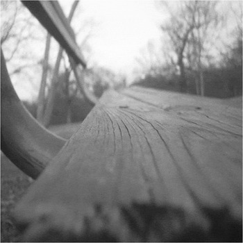
The visual system is highly sensitive to changes in luminance with position, which allows for the detection of lines and edges. The effects of changes in luminance contrast on the responses of retinal ganglion cells (RGCs) have been extensively studied. Edges in the natural environment, however, are not always sharp and may be blurred due to depth relative to fixation, motion, or shadows. The visual system is highly sensitive to out-of-focus objects and can easily detect and discriminate between focused and unfocused stimuli (Hamerly & Dvorak, Reference Hamerly and Dvorak1981; Watt & Morgan, Reference Watt and Morgan1983; Wang & Ciuffreda, Reference Wang and Ciuffreda2005a,Reference Wang and Ciuffredab). The ability to detect and discriminate blur serves as an advantage as blur has been found to be a useful cue in depth perception (Pentland, Reference Pentland1987; Mather & Smith, Reference Mather and Smith2000). For example, Fig. 1 shows a scene where objects at the point of fixation are sharp, but outside of the plane of fixation, elements are blurred as a function of distance from fixation, which gives a sense of depth.
In the visual environment, objects at the plane of fixation appear sharp. However, elements outside the fovea are variably blurred depending on the distance from fixation.

Reducing the contrast of a stimulus causes a decrease in spike rate and an increase in latency in retinal ganglion (Shapley & Victor, Reference Shapley and Victor1978; Sestokas et al, Reference Sestokas, Lehmkuhle and Kratz1991) and visual cortical neurons (Sclar & Freeman, Reference Sclar and Freeman1982; Reid et al., Reference Reid, Victor and Shapley1992; Albrecht, Reference Albrecht1995; Gawne et al., Reference Gawne, Kjaer and Richmond1996; Carandini et al., Reference Carandini, Heeger and Movshon1997; Gawne, Reference Gawne1999, Reference Gawne2000). In both retina and cortex, the resultant increase in latency produced by decreasing contrast is separable from the decrease in spike rate, which suggests that the visual system might use differential latency as a cue to encode relative stimulus contrast. Because blurring an object has the subjective effect of reducing contrast, blurring an edge might have similar effects as reducing contrast.
We have shown previously that increasing blur over a substantial range has negligible effects on the responses of visual cortical neurons (Risner & Gawne, Reference Risner and Gawne2009). However, if an edge is blurred to an extended degree, the spike rate of visual cortical neurons decreases (Siguenza et al., Reference Siguenza, Heide and Creutzfeldt1987). Ikeda and Hill (Reference Ikeda and Hill1971) examined the effects of blur, induced by corrective lenses, on the spike rate of individual cat RGCs. When stimuli were positioned in the center of a receptive field, spike rate decreased as blur increased. However, they did not assess the affect of blur on response latency.
The purpose of this study was to examine the responses of rabbit RGCs to edges varying in both contrast and blur. We present data from brisk-transient and brisk-sustained RGCs because the physiology of these cells have been extensively examined (Barlow et al., Reference Barlow, Hill and Levick1964; Caldwell & Daw, Reference Caldwell and Daw1978; Vaney et al., Reference Vaney, Levick and Thibos1981; Amthor et al., Reference Amthor, Takahashi and Oyster1989a; DeVries & Baylor, Reference DeVries and Baylor1997; Zeck & Masland, Reference Zeck, Xiao and Masland2007). Furthermore, brisk-transient and brisk-sustained cells show short interspike intervals, which suggest that these cells are likely to trigger action potentials in the lateral geniculate nucleus (Usrey et al. Reference Usrey, Reppas and Reid1998; Levine & Cleland, Reference Levine and Cleland2001; Sinich et al., Reference Sinich, Adams, Economides and Horton2007). Cells that trigger action potentials in downstream visual pathways are of great interest because previously, we have made recordings in area V1 of nonhuman primate assessing the responses to blurred edges (Risner & Gawne, Reference Risner and Gawne2009). However, 14 ganglion cell types have been identified in the rabbit retina (Marc & Jones, Reference Marc and Jones2002), and these remaining cells undoubtedly contribute a significant role in visual processing (see Koch et al., Reference Koch, McLean, Segev, Freed, Berry, Balasubramanian and Sterling2006).
Here, we show that not only is the spike rate of most RGCs attenuated by blurring an edge but also latency tends to increase as blur increases for most cells. For many neurons, blurring a high-contrast edge is similar to reducing the contrast of a sharp edge, suggesting that for these neurons, increasing blur has the same effect as decreasing contrast. Based on the population average, blur does not significantly affect latency, spike rate, or interspike interval until the edge is highly blurred (>2.9 deg of visual angle). Also, we tested the linearity of brisk-transient and brisk-sustained RGC responses to blurred edges by comparing the responses obtained from stimuli that were the pixel-by-pixel difference between a sharp edge and each blurred edge to the difference responses to a sharp edge and each blurred edge. A RGC was defined as linear if the response to a sharp edge was equal to the sum of the response to a blurred edge and the response to the differences between a sharp and blurred edge presented separately. We found that most brisk-sustained cells exhibit linear responses to blurred edges, and brisk-transient cells produce a mixture of linear and nonlinear responses to blurred edges. Some of these data have been previously reported in abstract form (Risner et al., Reference Risner, Nowak, Amthor and Gawne2009).
Materials and methods
Animals and surgical procedures
All of the following methods were approved by the Institutional Animal Care and Use Committee of the University of Alabama at Birmingham and are similar to the methods reported by Renna et al. (Reference Renna, Strang, Amthor and Keyser2007). Male and female New Zealand rabbits, weighing at least 1.3 kg, were anesthetized by intraperitoneal injections of urethane (1.53 g/kg), with a dosage frequency of three injections given 20 min apart. Under dim red light, Nembutal (Ovation Pharmaceuticals, Lake Forest, IL) was administered by way of the marginal ear vein and was given until no reflexive response could be elicited by a paw pinch. The eye was then enucleated and the animal was euthanized by an intravenous injection of 1 ml Fatal Plus (Vortech Pharmaceuticals, Dearborn, MI).
The eye was hemisected in ice-cold oxygenated bicarbonate-buffered Ames solution, the lens and vitreous were removed, and the retina was cut in half. One half of the eyecup was mounted on a domed chamber where heated (34–35°C) 95% O2 5% CO2 bicarbonate-buffered Ames solution (pH = 7.0–7.4) was superfused over the retinal surface at a rate of 2.5 ml/min.
Electrophysiology, receptive field mapping, and cell classification
Ganglion cell bodies were lightly stained with Azure B (Amthor et al., Reference Amthor, Keyser and Dmitrieva2002). Extracellular single-cell recordings were made near ganglion cell bodies using 0.6–0.7 MΩ carbon fiber–tipped copper wire in-glass electrodes plated with silver chloride (Armstrong-James & Millar, Reference Armstrong-James and Millar1979). Action potentials were amplified (Mentor, Minneapolis, MN) and filtered through a learning filter to remove 60 Hz (Riverbend Electronics, Rushford, MN). Spikes passing a threshold set by a Schmitt trigger were digitized at a sampling rate of 1 kHz. We verified that action potentials stemmed from a single cell by observing the height of each action potential (viewed on a digital oscilloscope) and the audio output.
For each ganglion cell, we carefully hand mapped the receptive field size and response bias (ON-, OFF-, or ON–OFF center) by flashing small high-contrast squares (70.75 cd/m2) on a dark background (0.03 cd/m2). The estimated size of receptive fields ranged from 1.45 to 8.12 deg of visual angle with a mean of 3.8 deg of visual angle. Most recordings were made near the fiber band of the retina.
All RGCs examined produced brisk responses to a high-contrast light square approximately the size of the center region of each cell’s receptive field, and responses had peak interspike intervals less than 20 ms (Amthor et al., Reference Amthor, Takahashi and Oyster1989a). RGCs were classified as brisk-transient or brisk-sustained post hoc based on the response duration produced by the same high-contrast square of light captured in the spike density function (see Data treatment and analysis for details). Cells were defined as brisk-transient if the firing rate decreased by 25% of the maximum response 150 ms after stimulus onset, and cells were defined as brisk-sustained if the firing rate was greater than 25% of the maximum response 150 ms after stimulus onset. A similar method for the classification of brisk-transient and brisk-sustained cells has been used previously (Amthor et al., Reference Amthor, Takahashi and Oyster1989a; Renna et al., Reference Renna, Strang, Amthor and Keyser2007). It has been noted by others that it can be difficult to distinguish between brisk-transient and brisk-sustained RGCs (especially in isolated retina preparations) (Caldwell & Daw, Reference Caldwell and Daw1978; Vaney et al., Reference Vaney, Levick and Thibos1981; Zeck & Masland, Reference Zeck and Masland2007). The extent of response duration is dependent on a number of factors outside of the intrinsic response properties of the cell, including level of light adaptation, temperature of the bath solution, and general health of the retina. This method of cell classification is thus similar to those previously employed to distinguish between cell classes (Amthor et al., Reference Amthor, Takahashi and Oyster1989a; Renna et al., Reference Renna, Strang, Amthor and Keyser2007).
Visual stimuli
All visual stimuli were presented on a computer monitor (DigiView, Model HR-78, Industry CA) measuring 33 cm wide and 23 cm in height with a refresh rate of 100 Hz. The monitor’s nonlinear relationship between command voltage and luminance was corrected by measuring the luminance of grayscale values using a photometer (Minolta, Model LS-110, Tokyo, Japan) and producing a color look-up table using the interp1 function in MATLAB (The Mathworks, Natick, MA). The image presented on the computer screen was reflected by a mirror located on top of the trinocular port of a microscope (Nikon, Model 179781, Tokyo, Japan) focused through the trinocular port, and projected onto the surface of the retina by way of a 4× objective. The demagnification of the projection through the microscope was 33:1. Each stimulus measured 50 × 200 pixels, which corresponds to approximately 3.5 × 14.5 deg of visual angle, where each pixel on the monitor was approximately 0.0725 deg of visual angle on the rabbit retina (Hughes, Reference Hughes1971). Nonsymmetrical stimuli were chosen so the edge could be blurred to a large extent (up to 180 pixels or 13.05 deg) but not to suppress the cell’s response by completely covering both the center and the surround regions of the receptive field.
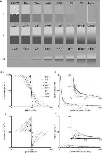
Visual stimuli consisted of sharp edges varied by contrast, high-contrast edges varied by degrees of blur, and the difference between a high-contrast sharp edge and each blurred edge (difference between sharp and blurred, DBSB) (Fig. 2A). Fig. 2Ai shows the sharp edges varied by contrast. Michelson contrast (L max − L min)/(L max + L min), where L max is the maximum luminance and L min is the minimum luminance, was varied from 85 to 0%. The maximum and minimum luminance values were 27.72 and 1.73 cd/m2, respectively. For some neurons, we also presented a white “frame,” which was the same size as the aforementioned stimuli, used to ensure that RGCs were responding to the transition in luminance of each stimulus and not to the sharp edges on the lateral flanks of each receptive field (see Fig 2Ai last column).
Visual stimuli used in this study and corresponding luminance profiles and spatial frequency spectra. Edges were flashed on for 1 s and off for 1 s during a data collection window of 2 s. The edges were positioned at the edge of the center region each receptive field (e.g., see dashed circle in Ai). (Ai) shows sharp edges varied by contrast from 85 to 0% Michelson contrast; the last stimulus in (Ai) is the high-contrast frame that was presented to ensure that cells were responding to the central edge of each stimulus and not to the sharp edges of the stimuli covering the lateral flanks of each cells receptive field. (Aii) shows high-contrast (85%) edges that were blurred from 0.73 to 13.05 deg visual angle on the rabbit retina. (Aiii) shows the difference between a high-contrast sharp edge and each blurred edge (DBSB stimuli). The DBSB stimuli contain the missing spatial frequencies between a high-contrast sharp edge and each blur profile. The background luminance was 10.63 cd/m2. (B) shows the luminance profiles of the (Bi) blurred edges and (Biii) DBSB stimuli as a function of pixel position. Spatial frequency spectra of the (Bii) blurred edges and (Biv) DBSB stimuli were obtained by multiplying the luminance functions with a Hamming window and taking the absolute value of the Fourier transform. The insets in (Bii) and (Biv) show spatial frequency spectra of the blurred edges and DBSB stimuli with the vertical axis expanded.

High-contrast (85%) blurred edges were produced by convolving a sharp edge with a disk filter of varying diameter. High-contrast edges were blurred from 0.73 to 13.05 deg of visual angle (Fig. 2Aii), which corresponds to positioning a sharp edge 53–23 cm in front of a fixation point at 57 cm, assuming an intact eye with a focal length of 13 mm (Hughes, Reference Hughes1972) and a pupil size of 3 mm. For an explanation of calculation of distance from fixation, see Risner and Gawne (Reference Risner and Gawne2009).
Fig. 2Bi shows the luminance function of each blurred edge. Blurred edges were similar to those used by Risner and Gawne (Reference Risner and Gawne2009) and Siguenza et al. (Reference Siguenza, Heide and Creutzfeldt1987), approximating a cosine function varied by width of the blur profile. For some of the experiments, the color depth of the monitor was 16 bit, which resulted in the most highly blurred edges exhibiting banding. For other experiments, the monitor’s color depth was 32 bit and there was no perceivable banding for any blur profile. We examined whether a cell responded differently to each blurred edge as a function of color depth, and there were no noticeable differences in spike rate or latency (see Fig. S1) perhaps because the banding was beyond the limits of the rabbit RGC’s ability to resolve.
To determine if the cells responded linearly or nonlinearly to blurred edges, we also presented the difference between the high-contrast (85%) sharp edge and each blur profile (DBSB stimuli Fig. 2Aiii). These stimuli were produced by taking the pixel-by-pixel difference of the high-contrast sharp edge and each blurred edge and adding the grayscale value corresponding to the stimulus background to avoid negative numbers. In other words, each DBSB stimulus is the difference between the sharp edge and a blurred edge. The luminance profile of each DBSB stimulus is shown in Fig. 2Biii. If a cell responds linearly, the difference between the response to the sharp edge and the response to each blurred edge should be similar to the response elicited by the corresponding DBSB stimulus.
The spatial frequency spectra of each blurred edge and DBSB stimulus were calculated by multiplying one vector of each luminance function by a Hamming window function and taking the absolute value of the fast Fourier transform. The luminance function was multiplied by a Hamming window function to avoid artifacts produced by sharp transitions at the edges of the stimuli that were outside of the receptive field extent. Fig. 2Bii and 2Biv shows the spatial frequency spectra for the blurred edge (Fig. 2Bii) and DBSB stimuli (Fig. 2Biv) on equal axes, demonstrating that the DBSB stimuli account for the missing frequencies between a sharp edge and each blurred edge. The insets in Fig. 2Bii and 2Biv show the spatial frequency spectra of each blurred edge and DBSB stimulus with the vertical axis expanded.
Stimulus placement and presentation
The center edge of each stimulus was focused and positioned near the edge of the center region of each receptive field so each neuron responded to the onset or offset of the white to gray transition (e.g., see white-dashed circle over the 85% contrast sharp edge in Fig. 2Ai). Stimuli were positioned near the edge of the receptive field so as much of the blur transition could be “seen” by the receptive field of each neuron. For some OFF-center and ON–OFF-center cells, we rotated the stimulus 180 deg and the cells responded to the onset of the black to gray transition. The relative response dynamics were similar regardless of the edge polarity (see Fig. S2). Stimuli were presented in a shuffled random order and were flashed on for 1 s and off for 1 s within a data collection window of 2 s for at least 10 trials per unique stimulus condition, although at least 30 trials per stimulus condition were collected for the majority of the cells. Stimuli were flashed on at time 500 ms and off at time 1500 ms. Stimulus timing was verified accurate to a single video frame by placing a photocell onto the computer monitor and recording the pulses generated by the onset of a flashed light stimulus.
Data treatment and analysis
Spike trains were convolved with a σ = 8 ms Gaussian kernel, which has the effect of low-pass filtering the spike density function with a cutoff of 16 Hz. Spike density functions have the advantage over poststimulus spike histograms in that only one variable need be assumed (σ), whereas one must assume a bin width and position when producing poststimulus spike histograms. Here, we chose the σ that allowed for the best resolution of data (i.e., there were no obvious peaks in the raw histograms filtered out by the Gaussian).
Response latency was defined as the time of half the maximum response of the spike density function within 250 ms poststimulus onset (500 ms) or offset (1500 ms) plus the average spike rate of the initial 500 ms for each stimulus case; adding the spike rate produced before stimulus onset ensures the half maximum of the spike density function was above the maintained discharge of the cell. Using the time to half-maximum response has the advantage that the number of trials per stimulus condition does not influence the measure of latency as compared to using the time where the response surpassed a particular standard deviation (Lee et al., Reference Lee, Williford and Maunsell2007). Furthermore, Levick (Reference Levick1973) examined the variability between different measures of latency of rabbit RGCs, comparing the variability of the first through fifth spike and 0.25–0.75 height of spike density function. He found that the half maximum of the spike density function was the measure that produced the least variability and increasing the width σ of the Gaussian between 6 and 10 ms did not alter the standard deviation of the half-maximum latency. Here, we express time of response latency as the latency value identified for each individual stimulus case minus the time of stimulus onset or offset. We normalized latency values by subtracting the mean latency value produced by each stimulus case from the mean latency produced by the high-contrast sharp edge for each cell, and this latency value is defined as the differential latency. For some cells, latency values could not be assigned for some stimulus cases (i.e., low contrast edges, highly blurred edges, and high spatial frequency DBSB stimuli) because few or no spikes were produced.
Spike rate was defined as the number of spikes within a 250 ms window after stimulus onset (500 ms) or offset (1500 ms) divided by the number of presentations for each unique stimulus. Spike rate was normalized by dividing the spike rate produced by each stimulus by the spike rate produced by the high-contrast sharp edge for each neuron.
Results
Response dynamics of RGCs to contrast or blur
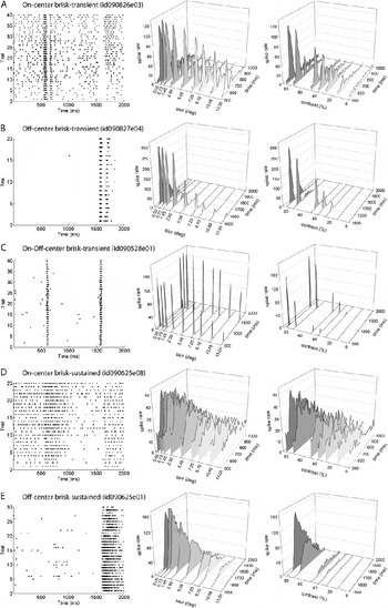
We made extracellular recordings from a total of 54 RGCs, including 13 ON-center brisk-transient, 13 OFF-center brisk-transient, 10 ON–OFF-center brisk-transient (nondirectionally selective), 10 OFF-center brisk-sustained, and 8 ON-center brisk-sustained cells. During recording, we also encountered three sluggish cells, but because so few of these cells were assessed, we will not discuss them in this report. Both brisk-transient and brisk-sustained RGCs produced robust responses to the high-contrast edges positioned near the edge of the center region of the receptive field. The first column in Fig. 3 shows raster plots exhibiting the responses of example cells to the 85% contrast sharp edge. The second column in Fig. 3 shows averaged spike density functions, for example, cells from each class and type as a function of degree of blur. As blur was increased, in general, responses decreased. Two cells, however, showed no decrease in spike rate to the blur series (one ON–OFF center brisk transient and one ON-center brisk sustained). The third column in Fig. 3 shows the responses of the same neurons to sharp edges varied by contrast. As expected, responses decreased as contrast decreased. For general interest, we present the raw traces of example neurons to selected experimental stimuli in Figs. S3–S5.
Responses of example neurons to edges varied by degrees of blur and sharp edges varied by contrast. Each row shows responses from an example RGC, including (A) ON-center brisk-transient, (B) OFF-center brisk-transient, (C) ON–OFF-center brisk-transient, (D) ON-center brisk-sustained, and (E) OFF-center brisk-sustained RGCs. The first column shows raw traces for each example neuron’s responses to the high-contrast sharp edge. The second column shows the average spike density functions, which is similar to a smoothed poststimulus histogram (see text for further details), to high-contrast edges varied by degrees of blur. The third column shows responses of the example neurons to sharp edges varied by contrast. For these example neurons, responses decreased as blur increased or contrast decreased. Stimuli were flashed on at 500 ms and off at 1500 ms.

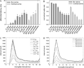
To assess the latency and spike rate as a function of blur and contrast, Fig. 4A and 4B shows a histogram of (Fig. 4A) differential latency and (Fig. 4B) normalized spike rate as a function of stimulus type pooled across all neurons in this study. Error bars show ±1 s.e.m. To determine if there was a significant effect of varying contrast or blur on the response dynamics, we performed a Kruskal-Wallis (KW) test of significance using the normalized values for latency and spike rate. The KW test, the nonparametric version of an analysis of variance, was chosen because the stimulus cases being compared contained unequal sample sizes. There were unequal samples between stimulus cases because latency values could not be defined for less salient stimuli, such as the sharp edges of lower contrast, highly blurred edges, and high spatial frequency DBSB stimuli. Because we used the normalized values in the statistical analysis, we did not include the stimulus (the 85% contrast/0 deg blur edge) that was used as the normalizing factor in the statistical analysis. As expected, we found a significant effect of contrast on spike rate (KW = 115.32, P < 0.0001) and latency (KW = 44.897, P < 0.0001). To determine the interactions, we used a two-tailed Dunn’s post hoc test, which showed that spike rates and latencies produced by a higher contrast sharp edge (70% contrast) were significantly different from those produced by lower contrast sharp edges (0–50%). Furthermore, we found a significant effect of blur on spike rate (KW = 199.10, P < 0.0001) and latency (KW = 91.254, P < 0.0001). Using the two-tailed Dunn’s post hoc test, we found that the response dynamics produced by smaller widths of blur (0.73–2.9 deg) were significantly different than the spike rates and latencies obtained by larger amounts of blur (7.25–13.05 deg). There was no significant difference between the 0% contrast (blank stimulus) and the white frame, t(4) = 0.156, P = 0.88, indicating that the cells were responding to the edges where blur and contrast were varied and not to the lateral sharp edges of the stimuli.
Histograms showing the (A) differential latency, (B) normalized spike rate, and (C and D) interspike interval distribution produced by each stimulus case. (A) Differential latency was defined as the difference between mean response latency produced by each stimulus case minus the mean latency produced by the 85% contrast sharp edge. (B) Spike rates were normalized by dividing the mean spike rate produced by each stimulus by the mean spike rate produced by the 85% contrast sharp edge. Error bars show ±1 s.e.m. (C and D) Interspike interval histogram based on the sum across all cells for each high-contrast blurred edge (C) and each sharp edge of varying contrast (D). The peak interspike interval was 4 ms across all blur and contrast profiles. Although there was a decrease in the number of short interspike intervals as blur increased or contrast decreased, the peak interspike interval remained constant and paralleled the reduction in spike rate.

We also assessed whether or not blur is encoded by the time between spikes. Fig. 4C and 4D shows histograms of the sum of interspike intervals across all cells for high-contrast edges varied by blur (Fig. 4C) and sharp edges of varying contrast (Fig. 4D). There was a decrease in shorter interspike intervals as blur was increased or contrast decreased; this decrease in shorter interspike intervals relates to the decrease in spike rate as blur was increased or contrast decreased. However, based on the interspike intervals across the population of neurons, there were no major shifts in peak interspike interval as a function of blur or contrast. The interspike interval histograms for individual cells showed a similar pattern (Fig. S6).
Examination of contrast equivalence
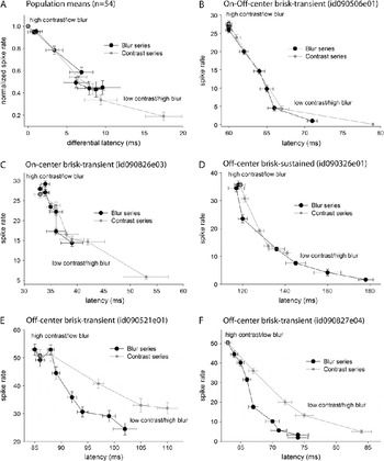
To determine if a given degree of blur can be related to a particular contrast, we plotted the contrast and blur series as a function of the normalized spike rate and differential latency values. On average, the response dynamics of RGCs are similar for blur and contrast, suggesting that blurring a high-contrast edge from 0.73 to 13.05 deg is, in general, comparable to decreasing the contrast of a sharp edge from 85 to 30% (Fig. 5A). Although the response dynamics of most individual RGCs were similar for blur and contrast (Fig. 5B–5D), there were some brisk-transient neurons that seem to encode blur and contrast differently (Fig. 5E and 5F); these OFF-center brisk-transient RGCs often produced shorter latencies to blur increments as compared to the longer latencies produced by contrast decrements.
Test of contrast equivalence for blurred edges based on the population average spike rate and latency values for all neurons in this study (A) and individual example RGCs (B–F). (A) The y-axis shows the normalized spike rate produced by each stimulus and the x-axis shows the differential latency obtained for each stimulus case. Black circles indicate data obtained for the blur series from a smaller degrees of blur (0 deg upper left) to a larger degrees of blur (13.05 deg lower right). The gray circles show data obtained for sharp edges varying by contrast from 85% (upper left) to 15% (lower right). (B–F) Examination of contrast equivalence for blurred edges for example cells. The y-axis shows spike rate values, and the x-axis shows latency values. For many individual cells, blurring a high-contrast edge is equivalent to decreasing the contrast of a sharp edge (B–D), but some cells encoded blur and contrast differently, producing shorter latencies (E–F) for blur increments as compared to the latencies obtained for decreasing the contrast of a sharp edge.

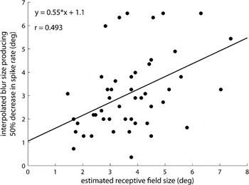
For many RGCs, the response dynamics were not altered until the edge was blurred greater than 2.9 deg of visual angle (i.e., there were no significant differences between spike rates and latencies produced by blurred edges ranging from 0.73 to 2.9 deg). One possible explanation for this finding is that the effective contrast of a stimulus is set by the range of luminance values within the receptive field, and blurring a stimulus only decreases the effective contrast when the blur is greater than the extent of the center of the receptive field. To investigate this idea, we plotted the estimated receptive field center size as a function of the interpolated blur size that produced a 50 ± 10% reduction in spike rate (Fig. 6). Four cells were excluded from this analysis because the spike rate of these neurons did not decrease by 50 ± 10% to the range of blur profiles. The receptive field size of these neurons that were excluded from this analysis ranged from 5.4 to 6.3 deg of visual angle, receptive field sizes that were smaller than the largest blur extent (13.05 deg); thus, the lack of reduction in spike rate as a function of increasing the size of blur cannot be explained by the high-contrast portion of the blurred edge extending beyond the center of the receptive field region. Although these cells produced anomalous responses compared to the population of RGCs, neurons insensitive to blur have also been found in rat retina (Powers & Green, Reference Powers and Green1978) and in the midbrain of rabbit (Lee & Hill, Reference Lee and Hill1972).
Receptive field center size is moderately correlated with a decrease in spike rate to blurred edges. The x-axis shows the estimated, hand-mapped receptive field center size for each cell; the y-axis shows the interpolated blur size that produced a 50 ± 10% decrease in spike rate. There was a moderate correlation between the two variable (r = 0.493). The solid line shows a best-fit linear regression model and the equation is stated in the upper left.

For the cells analyzed (n = 50), there was a moderate correlation (r = 0.493) between the estimated receptive field size and the interpolated degree of blur that reduced spike rate by 50 ± 10%, and the slope of the linear-fit line was significantly different from zero, F(1, 48) = 15.41, P = 0.0001. This finding suggests that some of the effects of blur may be accounted for by moving the extreme luminance values away from the receptive field extent.
Test of linearity
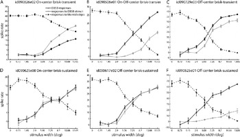
We also assessed the linearity of the responses to blurred edges by comparing the responses evoked by difference between sharp and blurred stimuli (responses to DBSB stimuli) and the difference between the responses evoked by a sharp edge and each blurred edge (DBSB responses). Fig. 7A–7F shows individual examples from each cell class and type. We found that many brisk-transient cells produced nonlinear responses to blurred edges (Fig. 7A and 7B). For these cells, there was a separation between the responses produced to the DBSB stimuli and the DBSB responses. However, there were brisk-transient cells that showed more linear responses (Fig. 7C). We found that most brisk-sustained cells exhibited linear responses to blurred edges (Fig. 7D and 7E). However, we did find one brisk-sustained cell that exhibited more nonlinear behavior (Fig. 7F).
Test of linearity for individual cell types, including (A) ON-center brisk-transient, (B) ON–OFF-center brisk-transient, (C) OFF-center brisk-transient, (D) ON-center brisk-sustained, and (E–F) OFF-center brisk-sustained RGCs. The dark open circles with dark solid lines show the difference of the responses to the high-contrast sharp edge and each blurred edge (DBSB responses). The gray open circles with gray solid lines show responses produced by difference between sharp edge and blurred edges (responses to DBSB stimuli). If a cell behaved linearly, then these two responses should superimpose. For comparison, the dark solid circles with dashed lines show responses produced by each edge varying by degrees of blur. Brisk-transient cells typically produced nonlinear responses to blurred edges (A and B), but many brisk-transient cells produced linear responses to blurred edges (C). Most brisk-sustained cells produced more linear responses to blurred edges (e.g., D–F), but one brisk-sustained cells produced nonlinear responses to high-contrast blurred edges (F).

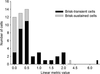
To view the distribution of linear and nonlinear responses produced by brisk-transient and brisk-sustained RGCs to blurred edges, we derived a linear metric, which was defined as the sum of the absolute difference between the responses to the DBSB stimuli and each DBSB response value divided by the absolute sum of DBSB stimulus values. A linear metric value of zero would indicate that a given cell was linear. Using the linear metric values, a histogram was produced using the histc function in MATLAB, which counted the frequency of linear metric values falling into each 0.25-wide bin. One OFF-center brisk-transient RGC was excluded from this analysis because no or few responses were elicited by the DBSB stimuli. Fig. 8 shows the distribution of brisk-transient (n = 35) and brisk-sustained (n = 18) cells as a function of the linear metric. There was a significant difference between the linear metric values for brisk-transient and brisk-sustained RGCs, Mann–Whitney U = 132.0, P < 0.001.
Linear metric to evaluate the distribution of linear and nonlinear brisk-sustained and brisk-transient RGCs. This metric was defined as the sum of the absolute difference between each DBSB stimulus normalized spike rate value and each DBSB response normalized spike rate value divided by the absolute sum of DBSB stimuli values. A linear metric value of zero would indicate that a given cell was linear.

Discussion
For most rabbit RGCs, as blur is increased or contrast is decreased, response latency increases and spike rate decreases. For many neurons, blurring a high-contrast edge has the same effect on spike rate and latency as lowering the contrast of a sharp edge. However, some brisk-transient cells respond differently to blur and contrast. These brisk-transient RGCs produced shorter latencies to increasing blur compared to decreasing contrast. We show that the receptive field center diameter is significantly correlated with a decrease in spike rate to blurred edges, suggesting that blur may affect the responses by removing the highest and lowest luminance values from the receptive field, thus in effect decreasing the stimulus contrast.
To test whether cells produced linear or nonlinear responses to blurred edges, we compared the responses produced by stimuli that represent the missing spatial components between a sharp edge and each blurred edge and the difference between the responses produced by a sharp edge and each blurred edge. Theoretically, if a cell responds linearly to blurred edges, the two should this be sets of values should be approximately equal. We found that brisk-transient cells produced both linear and nonlinear responses to blurred edges, whereas most brisk-sustained cells produced more linear responses to blurred edges. This is contradictory to our findings in visual cortex where all cells exhibited nonlinear behavior to a similar stimulus set (Risner & Gawne, Reference Risner and Gawne2009).
The response dynamics of RGCs to blur or contrast
Across the population of RGCs blurring, a high-contrast sharp edge is often similar to decreasing the contrast of a sharp edge based on response strength and latency. However, on average and for many individual RGCs, the response dynamics of RGCs to blurred edges are not significantly altered until the edge is blurred greater than 2.9 deg of visual angle. Although the smaller degrees of blur could be seen by the experimenters, the response dynamics of RGCs, on average, are not significantly affected by smaller amounts of blur (range 0.73–2.9 deg of visual angle). Furthermore, even the subpopulation of cells that appear to encode blur differently than contrast failed to show significant differences in response latencies or spikes rates compared to those produced by the high-contrast sharp edge (see Fig. 5E). In fact, many cells responded more robustly to a slightly blurred edge than a sharp edge (see Fig. 5B–5E); others have found similar results in visual cortex (Siguenza et al., Reference Siguenza, Heide and Creutzfeldt1987). Similarly, we have previously shown that neither spike rate, interspike interval, nor latency is affected by blurring an edge from 0.04 to 0.36 deg in primate V1 cells. Furthermore, Siguenza et al. (Reference Siguenza, Heide and Creutzfeldt1987) found that cat striate cortical cells are unable to distinguish between a sharp edge and an edge blurred up to 4 deg, a blur width well beyond the blur detection threshold predicted based on the acuity of the cat. These results beg the question: why are retinal ganglion and early visual cortical neurons insensitive to smaller degrees of blur?
It is assumed that the size and arrangement of RGC receptive fields set the limits of spatial resolution and therefore influence detecting blur. The rabbit visual streak contains many cell types and receptive field sizes ranging from 1 to 2 deg (Levick, Reference Levick1967), and many types of RGCs partially overlap, enhancing spatial resolution without an excessive amount of redundancy (DeVries & Baylor, Reference DeVries and Baylor1997). The behavioral grating visual acuity of the rabbit is approximately 3 cycles/deg (van Hof, Reference van Hof1967; Vaney, Reference Vaney1980), which is 10 times below the grating acuity in humans. Although the blur detection threshold of the rabbit is unknown, the blur detection threshold in human is between 0.33 min arc (0.0056 deg) and 0.5 min arc (0.0083 deg) (Hamerly & Dvorak, Reference Hamerly and Dvorak1981). The blur detection threshold of the rabbit may be estimated, based on the grating acuity of the rabbit, to be about 0.08 deg, a threshold lower than that estimated based on the data in the present study, but neurons here were located near the visual streak or middle periphery and would likely be less sensitive to blur than RGCs located in the visual streak, which set the limits of visual acuity.
Another class of rabbit RGCs, local-edge detectors (LEDs), may be involved in detecting blur. LEDs have small receptive fields, which partially overlap, separated from neighboring LEDs by 30–40 μm (Levick, Reference Levick1967; Amthor et al., Reference Amthor, Takahashi and Oyster1989b; DeVries & Baylor, Reference DeVries and Baylor1997; van Wyk et al., Reference van Wyk, Taylor and Vaney2006), a separation nearly sufficient to account for the grating acuity (van Hof, Reference van Hof1967; Vaney, Reference Vaney1980; van Wyk et al., Reference van Wyk, Taylor and Vaney2006). LEDs are most sensitive to lines and edges of rapid changes in contrast and are most sensitive to higher spatial frequencies (0.3–1.5 deg), exhibiting narrow spatial frequency bandpass but are suppressed by gratings most likely due to strong inhibitory surround input (Zeck et al., Reference Zeck, Xiao and Masland2005). These characteristics of LEDs make them a candidate cell type to detect shorter widths of blur by detecting sharp changes in a luminance function separated by a more gradual change in luminance (i.e., a blurred edge).
Another possible explanation for the finding that the response dynamics are not altered by smaller amounts of blur is that the effective contrast of the stimulus is the same for smaller blurs, and the responses of the ganglion cells are normalized by the contrast of the stimulus. The effective stimulus contrast has been shown to set the gain or normalize both retinal ganglion (Shapley & Victor, Reference Shapley and Victor1978, Reference Shapley and Victor1979, Reference Shapley and Victor1980, Reference Shapley and Victor1981) and visual cortical cell responses (Ohzawa et al., Reference Ohzawa, Sclar and Freeman1985; Bonds, Reference Bonds1991; Albrecht, Reference Albrecht1995; Carandini et al., Reference Carandini, Heeger and Movshon1997), and these contrast gain control mechanisms may account for the perceptual phenomenon of contrast constancy (Georgeson & Sullivan, Reference Georgeson and Sullivan1975). To investigate the idea that the responses of RGCs to blurred edges are normalized by the effective contrast of the stimulus, we plotted the estimated receptive field center size as a function of the blur size that produced a 50 ± 10% reduction in spike rate. The idea behind this analysis was if the size of the blurred edge exceeded the estimated size of the center of the receptive field, then that would suggest that the high-contrast portion of the blurred edge would extend beyond the center of the receptive field and the effective contrast of the stimulus would be reduced. As shown in Fig. 6, the blur size that produced 50% reduction of spike rate was plotted as a function of the receptive field, and there was a significant correlation, suggesting that when the high-contrast portion of the edge extended beyond the center of the receptive field, there was a dramatic decrease in spike rate. The actual correlation between the amount of blur causing a criterion decrease in spike rate and receptive field size could be greater for a number of reasons. First, we only estimated receptive field size by hand mapping. Second, we placed the edge of the stimulus near the edge of the receptive field and not at the end of the receptive field center region. Third, we are comparing the responses across the population of both brisk-transient and brisk-sustained cells. Finally, the surround contribution to overall output of the cells varies from cell-to-cell. However, this only moderate correlation may suggest that the peripheral area of the receptive field contributed to the total response to blurred edges.
Contrast equivalence
The ability to discriminate blur decreases as contrast decreases (Westheimer et al., Reference Westheimer, Brincat and Wehrhahn1999). But if contrast is held constant, does the perceived contrast of a stimulus decrease as blur increases? Marmor and Gawande (Reference Marmor and Gawande1988) found that contrast sensitivity decreases as optical defocus increases. In corroboration with human psychophysical studies, Ikeda and Hill (Reference Ikeda and Hill1971) showed that blurring a spot by adding corrective lenses may be related to decreasing the contrast of a spot of light based on the spike rate of a RGC. Here, we extend this idea, showing that blurring an edge can often be similar to reducing the contrast based on both the spike rate and the latency (see Fig. 5A–5D). However, some OFF-center brisk-transient cells respond differently to blur and contrast, suggesting there is a subset of brisk-transient RGCs that may directly encode blur (see Fig. 5E and 5F). These OFF-center brisk-transient RGCs produced shorter response latencies to blur increments as compared to the latencies produced by contrast decrements. Although these OFF-center brisk-transient RGCs do encode blur differently than contrast, this experimental result may reflect an asymmetry between the effects of contrast gain control on ON-center and OFF-center cells, where ON-center cells are more tightly governed by a gain control mechanism than OFF-center cells in both retina and lateral geniculate nucleus (Chander & Chichilnisky, Reference Chander and Chichilnisky2001; Zaghloul et al., Reference Zaghloul, Boahen and Demb2005; Bronin et al., Reference Bronin, Mante and Carandini2006).
Test of linearity
The systems approach of spatial frequency analysis has been widely employed to investigate the receptive field properties of RGCs (for a review, see Shapley & Lennie, Reference Shapley and Lennie1985). These studies usually use sinusoidal gratings, a stimulus that consists of a single spatial frequency, to probe the receptive field properties of cells. One important property often examined is the linearity of superposition. Linearity is important because if a cell behaves as a linear filter, then the cell’s responses can be predicted to a given stimulus set. Spatial frequency analysis has shown that rabbit brisk-type RGCs are similar to cat and can be separated into linear and nonlinear types (Enroth-Cugell & Robson, Reference Enroth-Cugell and Robson1966; Caldwell & Daw, Reference Caldwell and Daw1978). However, Amthor et al. (Reference Amthor, Takahashi and Oyster1989a) found a subpopulation of brisk-transient cells that exhibited linear behavior to contrast reversing patterns.
Although, spatial frequency analysis is a powerful tool, drifting sinusoidal gratings are not natural stimuli, and even though cells may be distinctly separated by responses to sinusoidal gratings under threshold condition, this separation of responses does not hold under natural, suprathreshold, conditions to edges of varying blur (Siguenza et al., Reference Siguenza, Heide and Creutzfeldt1987). In this study, we examined the linearity of rabbit RGCs to blurred edges, which are general features of the natural environment, flashed on and off within the receptive fields of RGCs under a moderately light-adapted condition. Because a sharp edge can be thought of as the sum of a blurred edge and the missing spatial frequencies, to test the linearity of RGCs, we presented stimuli that were the pixel-by-pixel difference between a sharp edge and each blurred edge (responses to DBSB stimuli), which represent the missing spatial frequencies between a sharp edge and each blurred edge and compared the spike rate produced by each DBSB stimulus to the difference between the spike rate produced by the sharp edge and each blurred edge (DBSB responses). Of course, cells could be separated into linear or nonlinear based on this metric, but our intention was to observe the linearity of responses of cells initially classified as brisk transient or brisk sustained by our conventional criteria (see Materials and methods). We found that most brisk-sustained cells produced linear responses. Brisk-transient cells, on the other hand, formed a near normal distribution, where cells produced both linear and nonlinear responses.
Conclusion
We investigated the spike rate and latency of brisk-transient and brisk-sustained RGCs to high-contrast edges of varying blur and sharp edges varied by contrast. Spike rate decreases and latency increases as edge contrast decreases or blur increases. However, on average, there is not a significant shift in spike rate or latency until an edge is extremely blurred (>2.9 deg visual angle). The lack of change in the response dynamics to smaller degrees of blur is most likely due to a contrast gain control mechanism where responses are normalized by the effective contrast of a stimulus within the receptive field. But when an edge is blurred to a high degree, the local contrast of the image is attenuated and the response dynamics are scaled to the new contrast. In corroboration with this idea, we found that blurring a high-contrast edge is similar to reducing the contrast of a sharp edge based on the average spike rate and latency values for most cells and across the population. However, some brisk-transient RGCs encode blur and contrast differently, where these brisk-transient cells produce smaller increases in latencies to blur increments as compared to the latency values produced by contrast decrements. Finally, we find that most brisk-sustained RGCs produce linear responses to blurred edges, whereas brisk-transient RGCs produced both linear and nonlinear responses to blurred edge, suggesting that there is a population of brisk-transient cells that behave linearly to more natural stimuli, such as edges varied by amount of blur.
Acknowledgments
This work was supported by the National Science Foundation grant IOB 0622318 (T.J.G.) and NIH EY03039 (UAB Vision Science Research Center Core). We wish to thank John Tootle for programming assistance and James Black for technical support. We appreciate the helpful suggestions made by Przemyslaw Nowak, Allan Dobbins, and Thomas Norton.