





1. Introduction
A variety of phenomena in fluid mechanics result from the release of a finite volume of viscous fluid, such as the flow of honey on a disk or the geological sequestration of carbon dioxide deep within the Earth (Huppert Reference Huppert2006; Huppert & Neufeld Reference Huppert and Neufeld2014; Ungarish Reference Ungarish2020). These flow patterns, known as viscous gravity currents, are characterized by the horizontal intrusion of a denser fluid into a domain occupied by a less dense fluid.
The propagation of viscous gravity currents has been successfully modelled using low-dimensional approaches based on lubrication theory, effectively capturing flow behaviour in both two-dimensional and axisymmetric configurations (Huppert Reference Huppert1982, Reference Huppert2006). These foundational models have facilitated further theoretical investigations, particularly into how factors such as fluid rheology and boundary conditions influence the flow dynamics. Understanding these effects is crucial, given the broad range of applications in geophysics, oceanography and chemical engineering.
Progress in fluid rheology has enhanced our understanding of non-Newtonian, power-law fluids in the context of viscous gravity currents. Sayag & Worster (Reference Sayag and Worster2013) studied the axisymmetric flow of power-law fluids, demonstrating that inertia dominates the early evolution, while viscosity takes control later. Longo, Di Federico & Chiapponi (Reference Longo, Di Federico and Chiapponi2015) investigated how channel geometry influences the spread of power-law fluid currents, highlighting that the channel shape plays a critical role in determining flow velocity and front position. Further, Longo et al. (Reference Longo, Chiapponi, Petrolo, Lenci and Di Federico2021) explored the radially convergent viscous gravity currents of power-law fluids, providing a second kind of self-similar solution that accurately predicts current fronts.
Boundary conditions also play a crucial role in the propagation of viscous gravity currents (Zheng & Stone Reference Zheng and Stone2022). For instance, over permeable surfaces, vertical drainage significantly alters the amount of fluid in the main flow, as demonstrated by Acton, Huppert & Worster (Reference Acton, Huppert and Worster2001) and later refined by Liu, Zheng & Stone (Reference Liu, Zheng and Stone2017) to include capillary effects. Over elastic surfaces, the dynamics shifts, with early-stage flows being gravity driven, while later stages flatten due to the surface stretching from accumulated liquid (Zheng, Griffiths & Stone Reference Zheng, Griffiths and Stone2015). Similarly, Howell et al. (Reference Howell, Kim, Popova and Stone2016) investigated thin films flowing over elastic beams, revealing distinct flow regimes influenced by beam deformation and gravitational forces. These mechanisms, such as vertical drainage and elastic deformation, largely depend on the current height, allowing for the application of low-dimensional models that yield similarity solutions.
While low-dimensional models have proven effective in many cases, their generality may be limited when applied to rigid curvilinear surfaces, particularly in both natural and engineering contexts, where the surface characteristic length scale becomes a dominant factor. Although previous studies, ranging from macro-scale gravity-driven lava flows on hillsides to micro-scale capillary-induced coating films in microelectronic devices (Kalliadasis, Bielarz & Homsy Reference Kalliadasis, Bielarz and Homsy2000; Saprykin et al. Reference Saprykin, Trevelyan, Koopmans and Kalliadasis2007; Hinton, Hogg & Huppert Reference Hinton, Hogg and Huppert2019; Saville, Hinton & Huppert Reference Saville, Hinton and Huppert2022), have focused on steady-state distributions of viscous flows over curvilinear surfaces, less attention has been paid to the unsteady evolution of these flows.
In this study, our focus is on the evolution and propagation of the viscous fluid over rigid curvilinear surfaces, resulting from a finite volume, before reaching its steady state. To represent curvilinear surfaces, we employ a linear–exponential shape for general single-peak surfaces and a sinusoidal shape for surfaces with continuous peaks. Both two-dimensional and axisymmetric configurations are explored.
The structure of the paper is as follows: § 2 develops low-dimensional models for viscous fluids over rigid curvilinear surfaces. Section 3 characterizes the two types of curvilinear surfaces and reveals a dimensionless parameter that reflects the interaction between the released fluid and the surface geometry. Section 4 examines current evolution and propagation over linear–exponential and sinusoidal surfaces. Section 5 provides numerical validation using computational fluid dynamics, and § 6 concludes the study.
2. Methodology
2.1. Two-dimensional propagation
In a semi-infinite two-dimensional domain with a rigid and impermeable curvilinear surface of shape  $f(x)$, a fluid with density
 $\rho _{0}$ and viscosity
 $\mu _{0}$ initially fills the space. Then, another denser fluid with density
 $\rho$ (
 $\rho >\rho _{0}$) and viscosity
 $\mu$ (
 $\mu >\mu _{0}$) is horizontally introduced from the left. Due to the density difference
 $\Delta \rho$, the fluid propagates along the curvilinear surface as a gravity current. If the fluid is highly viscous and no capillary effect exists between the two fluids (the Bond number,
 $Bo = \Delta \rho gl^2/\sigma \gg 1$, where g is the acceleration due to gravity,
 $l$ is a characteristic length and
 $\sigma$ is the surface tension), the viscous gravity current propagates slowly with a sharp interface, represented by
 $h(x,t)$, as illustrated in figure 1.
Schematic diagram of a viscous gravity current over an impermeable and rigid curvilinear surface.

We assume that the curvature of the curvilinear surface is sufficiently small, rendering the centrifugal force induced by the curvature negligible. Additionally, while curvature primarily influences the pressure distribution normal to the surface, under the thin-film approximation, the film thickness is much smaller than the radius of curvature. As a result, the impact of curvature on the normal pressure gradient is minimal. Moreover, regarding the tangential pressure gradient, the effect of curvature is even less significant, because the liquid film is primarily driven by the surface gradient. Therefore, in our modelling, we disregard the effect of curvature and focus instead on the dominant influence of the surface gradient on the flow.
Regarding surface gradient, the shape of the curvilinear surface primarily influences the horizontal pressure gradient by altering the hydrostatic pressure distribution within the fluid. Strictly speaking, the fluid should flow tangentially along the curvilinear surface, which implies that the pressure gradient should be taken in the tangential direction when constructing the lubrication model. However, we consider the surface gradient to be limited, so that the difference between the tangential and horizontal directions are negligible. Consequently, the main contribution to the pressure gradient arises from changes in hydrostatic pressure relative to the horizontal position. Therefore, we approximate the horizontal flow  $\boldsymbol{u}(z,t)$ over the curvilinear surface using the classical lubrication model, where the balance is maintained between the horizontal pressure gradient and the viscous shear in the vertical direction in global coordinate system
 \begin{equation} \frac{\partial p}{\partial x}=\mu\frac{\partial^{2}\boldsymbol{u}}{\partial z^{2}}. \end{equation}
During current propagation, the pressure field is considered as hydrostatic
 \begin{equation} p(x,z)=p_{0}+\rho_{0} g[D-h(x,t)-f(x)]+\rho g[h(x,t)+f(x)-z], \end{equation}
therefore
 \begin{equation} \frac{\partial p}{\partial x}=\rho g_{0}\left(\frac{\partial h}{\partial x}+ \frac{{\rm d}\kern0.08em f}{{\rm d}\kern0.06em x}\right), \end{equation}
where  $p_{0}$ is atmospheric pressure,
 $D$ is the total liquid depth and
 $g_{0}=(\Delta \rho /\rho )g$ is the reduced gravity. The term
 ${\rm d}\kern0.08em f/{{\rm d}\kern0.06em x}$ indicates the contribution of the curvilinear surface, altering the gravity-driven influence of the current height.
The current velocity field can be derived with two boundary conditions, including the no-slip condition ( $\boldsymbol{u}=0$ at
 $z=f$) and the continuous shear stress at the interface (
 $\partial \boldsymbol{u}/\partial z=0$ at
 $z=h+f$), to obtain
 \begin{equation} \boldsymbol{u}=\frac{1}{2\mu}\frac{\partial p}{\partial x}[z^{2}-2z(h+f)+2hf+f^{2}]. \end{equation}
Utilizing the volume continuity equation for an incompressible current, we obtain
 \begin{equation} \frac{\partial h}{\partial t}+\frac{\partial}{\partial x}\left(\int_{f}^{h+f}\boldsymbol{u}\,{\rm d} z\right)=0. \end{equation}
Therefore, the low-dimensional model for the height of a viscous gravity current is established as
 \begin{equation} \frac{\partial h}{\partial t}-\beta\frac{\partial}{\partial x}\left[h^{3} \left(\frac{\partial h}{\partial x}+\frac{{\rm d} f}{{\rm d}\kern0.06em x}\right)\right]=0, \end{equation}
where  $\beta =g_{0}/(3\nu )$ and
 $\nu =\rho /\mu$. With the above simplification, we have effectively addressed the complex problem of flow over a curvilinear surface by accounting for the impact of the surface gradient on the hydrostatic pressure distribution, making it more practical for analysing and predicting the evolution of the viscous fluid over curvilinear surfaces.
The low-dimensional model has physical constraints for the front of the current, denoted as  $x_{f}(t)$,
 \begin{equation} h[x_{f}(t),t]=0 \end{equation}
and the volume conservation over time
 \begin{equation} \int_{0}^{x_{f}(t)}h\,{\rm d}\kern0.06em x=q, \end{equation}
where  $q$ is a constant for the release of a finite volume of fluid.
While the current front is moving,  $x_{f}(t)$ is an unknown parameter that makes it difficult to directly resolve the low-dimensional model. In spite of this, due to the fact that no current exists in the region from the current front to the right end of the domain,
 $[x_{f}(t),l]$, the right boundary condition can be transformed to
 \begin{equation} h(l,t)=0, \end{equation}
and then, the volume conservation equation is updated to
 \begin{equation} \int_{0}^{l}h\,{\rm d}\kern0.06em x=q. \end{equation}
After integrating the low-dimensional model and meanwhile utilizing the right boundary, the left boundary condition is obtained
 \begin{equation} \left.\left(\frac{\partial h}{\partial x}+\frac{{\rm d} f}{{\rm d}\kern0.06em x}\right)\right|_{x=0}=0. \end{equation}
We consider a finite-volume viscous fluid placed in a square with an initial height  $h_{0}$ and length
 $x_{0}$ (
 $x_{0}= q/h_{0}$) at
 $t=0$, where
 \begin{equation} h(x,0)=\begin{cases} h_{0} & 0\leq x\leq x_{0}\\ 0 & x>x_{0}. \end{cases} \end{equation}
The above boundary and initial conditions complete the low-dimensional model for the two-dimensional propagation of a viscous gravity current over an impermeable and rigid curvilinear surface.
2.2. Axisymmetric propagation
Similarly, for the axisymmetric propagation of viscous gravity currents with height  $h(r, t)$ over a rigid curvilinear surface
 $f(r)$, the local volume continuity balance equation is written as
 \begin{equation} \frac{\partial h}{\partial t}+\frac{1}{r}\frac{\partial}{\partial r}\left(r\int_{f}^{h+f}\boldsymbol{u}\,{\rm d} z\right)=0. \end{equation}
Because the axisymmetric hydrostatic pressure field is expressed as
 \begin{equation} p(r,z)=p_{0}+\rho_{0} g[D-h(r,t)-f(r)]+\rho g[h(r,t)+f(r)-z], \end{equation}
and its radial gradient is
 \begin{equation} \frac{\partial p}{\partial r}=\rho g_{0} \left(\frac{\partial h}{\partial r}+ \frac{{\rm d} f}{{\rm d} r}\right)=\mu\frac{\partial^{2}\boldsymbol{u}}{\partial z^{2}}, \end{equation}
the low-dimensional model for the height of an axisymmetric viscous gravity current is finally established as
 \begin{equation} \frac{\partial h}{\partial t}-\frac{\beta}{r}\frac{\partial}{\partial r} \left[rh^{3}\left(\frac{\partial h}{\partial r}+\frac{{\rm d} f}{{\rm d} r}\right)\right]=0. \end{equation}
Similar to the two-dimensional propagation, by transforming the domain from  $[0,r_{f}(t)]$ to
 $[0,l]$, the updated right boundary condition and the volume conservation equation are
 \begin{equation} h[r_{f}(t),t]=h[l,t]=0 \end{equation}
and
 \begin{equation} 2{\rm \pi}\int_{0}^{r_{f}(t)} rh\,{\rm d} r=2{\rm \pi} \int_{0}^{l} rh\,{\rm d} r=q. \end{equation}
Accordingly, the left boundary condition can be written as
 \begin{equation} \left.\left(\frac{\partial h}{\partial r}+\frac{{\rm d} f}{{\rm d} r}\right)\right|_{r=0}=0. \end{equation}
We consider a finite volume of viscous fluid placed in a cylinder with an initial height  $h_{0}$ and radius
 $r_{0}=\sqrt {q/({\rm \pi} h_{0})}$ at
 $t=0$, represented by
 \begin{equation} h(r,0)=\begin{cases} h_{0} & 0\leq r\leq r_{0}\\ 0 & r>r_{0}. \end{cases} \end{equation}
The above establishes the low-dimensional model for the axisymmetric propagation of a viscous gravity current over an arbitrary impermeable and rigid curvilinear surface.
2.3. Volume of fluid method
We utilize computational fluid dynamics (CFD) to validate low-dimensional models. Considering a sharp interface of a viscous gravity current separating two fluids during its propagation, the volume of fluid (VOF) method can be employed, which has been a widely used numerical method for two-phase flows. The capillary effects, which are neglected in low-dimensional models, are constructed by the continuous surface force model. The incompressible version of the VOF method is as follows (Hirt & Nichols Reference Hirt and Nichols1981):
 $$\begin{gather} \boldsymbol{\nabla}\boldsymbol{\cdot}\boldsymbol{u}=0, \end{gather}$$
 $$\begin{gather}\frac{\partial(\rho\boldsymbol{u})}{\partial t}+\boldsymbol{\nabla}\boldsymbol{\cdot}(\rho\boldsymbol{u}\boldsymbol{u})=-\boldsymbol{\nabla} p+\mu\nabla^{2}\boldsymbol{u}+\rho\boldsymbol{\boldsymbol{g}} +\sigma \boldsymbol{\nabla}\boldsymbol{\cdot}\left(\frac{\boldsymbol{\nabla} \alpha}{|\boldsymbol{\nabla} \alpha|}\right)\boldsymbol{\nabla} \alpha, \end{gather}$$
 $$\begin{gather}\frac{\partial \alpha}{\partial t}+\boldsymbol{\nabla}\boldsymbol{\cdot}(\boldsymbol{\boldsymbol{u}}\alpha)+ \boldsymbol{\nabla}\boldsymbol{\cdot} \left[\alpha(1-\alpha)\left(C|\boldsymbol{\boldsymbol{u}}|\frac{\boldsymbol{\nabla} \alpha}{|\boldsymbol{\nabla} \alpha|}\right)\right]=0, \end{gather}$$
where  $\boldsymbol {u}$ and
 $p$ are the uniform velocity and pressure fields,
 $\alpha$ is the phase fraction and
 $C$ is an artificial compressed factor to ensure a numerically sharp interface. Furthermore, turbulence effects may have a significant impact on the two-phase flow behaviour as the flow reaches higher Reynolds numbers, which, however, are neglected in this study of viscous gravity currents at low Reynolds numbers. Therefore, we do not consider turbulence modelling.
3. Non-dimensionalization
To construct a curvilinear surface, we consider a linear–exponential shape featuring a single peak, represented by  $f(x)=ax\,{\rm e}^{-bx}$ and
 $f(r)=ax\,{\rm e}^{-br}$, for both two-dimensional and axisymmetric propagation, and then broaden to a simple sinusoidal surface with multiple peaks, represented by
 $f(x)=a[1-\cos (\lambda x)]$ and
 $f(r)=a[1-\cos (\lambda r)]$, for which viscous fluids eventually stop, no matter how much volume is released. For generality, we carry out non-dimensionalization to enable a fundamental understanding of the flow system.
3.1. Two-dimensional propagation
We use the following scalings for two-dimensional linear–exponential surfaces:
 \begin{equation} S_{x}=1/b,\quad S_{h}=a/b,\quad S_{t}=b /(\beta a^{3}) \end{equation}
and the following scalings for sinusoidal surfaces
 \begin{equation} S_{x}=1/\lambda,\quad S_{h}=A,\quad S_{t}=1/(\beta \lambda^{2}A^{3}), \end{equation}
where
 \begin{equation} x=XS_{x},\quad h=HS_{h},\quad t=TS_{t}. \end{equation}
Subsequently, we derive a unified non-dimensional model
 $$\begin{gather} \frac{\partial H}{\partial T}-\frac{\partial}{\partial X} \left[H^{3}\left(\frac{\partial H}{\partial X}+\frac{{\rm d} F}{{\rm d}\kern0.06em X}\right)\right]=0, \end{gather}$$
 $$\begin{gather}\int_{0}^{L}H\,{\rm d}\kern0.06em X=M, \end{gather}$$
 $$\begin{gather}\left.\left(\frac{\partial H}{\partial X}+\frac{{\rm d} F}{{\rm d}\kern0.06em X}\right)\right|_{X=0}=0, \end{gather}$$
 $$\begin{gather}H(L,T)=0, \end{gather}$$
 $$\begin{gather}H(X,0)=\begin{cases}H_{0} & 0\leq X\leq X_{0}\\ 0 & X > X_{0}, \end{cases} \end{gather}$$
 $$\begin{gather}X_{0}=M/H_{0}. \end{gather}$$
Accordingly, the non-dimensional forms of the two-dimensional linear–exponential and sinusoidal surfaces are expressed as  $F(X)=X\,{\rm e}^{-X}$ and
 $F(X)=1-\cos (X)$.
From the non-dimensional model, the flow system is governed by two dimensionless parameters,  $M$ and
 $H_{0}$. Therein,
 $M$ represents the non-dimensional volume of the released viscous fluid and
 $H_{0}$ determines the non-dimensional initial height of the released volume. Moreover, the
 $M$ for both two-dimensional linear–exponential and sinusoidal surfaces is defined as
 \begin{equation} M=\begin{cases}
qb^{2}/a & F(X)=X\,{\rm e}^{-X}\\
\lambda q/A & F(X)=1-\cos(X). \end{cases}
\end{equation}
Because the volume of the two-dimensional linear–exponential surface,  $A_{e}$, and the volume of one wavelength on the two-dimensional sinusoidal surface,
 $A_{s}$, are calculated as
 $$\begin{gather} A_{e}=a\int_{0}^{+\infty}x\,{\rm e}^{-bx}\,{{\rm d}\kern0.06em x}=a/b^{2}, \end{gather}$$
 $$\begin{gather}A_{s}=A\int_{0}^{2{\rm \pi}/\lambda}[1-\cos(\lambda x)]\,{{\rm d}\kern0.06em x}=2{\rm \pi} A/\lambda, \end{gather}$$
 $M$ can be reconstructed as
 \begin{equation} M= \begin{cases}
q/A_{e} & F(X)=X\,{\rm e}^{-X}\\
2{\rm \pi} q/A_{s} & F(X)=1-\cos(X) , \end{cases}
\end{equation}
indicating that  $M$ represents the two-dimensional volume ratio between the released viscous fluid and the two-dimensional linear–exponential or sinusoidal surface.
3.2. Axisymmetric propagation
Using the same scalings as in two-dimensional propagation for both curvilinear surfaces, we obtain
 $$\begin{gather} S_{r}=1/b,\quad S_{h}=a/b,\quad S_{t}=b /(\beta a^{3}), \end{gather}$$
 $$\begin{gather}S_{r}=1/\lambda,\quad S_{h}=A,\quad S_{t}=1/(\beta \lambda^{2}A^{3}), \end{gather}$$
where
 \begin{equation} r=RS_{r},\quad h=HS_{h},\quad t=TS_{t}, \end{equation}
and thus the non-dimensional model for axisymmetric propagation is
 $$\begin{gather} \frac{\partial H}{\partial T}-\frac{1}{R}\frac{\partial}{\partial R} \left[RH^{3}\left(\frac{\partial H}{\partial R}+\frac{{\rm d} F}{{\rm d} R}\right)\right]=0, \end{gather}$$
 $$\begin{gather}2{\rm \pi}\int_{0}^{L} RH\,{\rm d} R=M, \end{gather}$$
 $$\begin{gather}\left.\left(\frac{\partial H}{\partial R}+\frac{{\rm d} F}{{\rm d} R}\right)\right|_{R=0}=0, \end{gather}$$
 $$\begin{gather}H(L,T)=0, \end{gather}$$
 $$\begin{gather}H(R,0)=\begin{cases}
H_{0} & 0\leq R\leq R_{0}\\
0 & R>R_{0}, \end{cases}
\end{gather}$$
 $$\begin{gather}R_{0}=\sqrt{M/({\rm \pi} H_{0})}. \end{gather}$$
Accordingly, the non-dimensional axisymmetric linear–exponential and sinusoidal surfaces are expressed as  $F(R)=R\,{\rm e}^{-R}$ and
 $F(R)=1-\cos (R)$.
Then, similar to the two-dimensional propagation, the dimensionless parameter  $M$ governs the flow system and the dimensionless parameter
 $H_{0}$ determines the initial condition. For axisymmetric linear–exponential and sinusoidal surfaces, the definition of
 $M$ is written as
 \begin{equation} M=\begin{cases}
qb^{3}/a & F(R)=R\,{\rm e}^{-R}\\
\lambda ^{2} q/A & F(R)=1-\cos(R). \end{cases}
\end{equation}
Because the three-dimensional volume of the axisymmetric linear–exponential surface,  $V_{e}$, is calculated as
 \begin{equation} V_{e}=2{\rm \pi} a\int_{0}^{+\infty} r^2\,{\rm e}^{-br}\,{\rm d} r=4{\rm \pi} a / b^{3}, \end{equation}
and the annular volume of the first wavelength on the axisymmetric sinusoidal surface,  $V_{s}$, which corresponds to
 $[0, 2{\rm \pi} /\lambda ]$, is calculated as
 \begin{equation} V_{s}=2{\rm \pi} A\int_{0}^{2{\rm \pi}/\lambda} r[1-\cos(\lambda r)]\,{\rm d} r=4{\rm \pi}^3 A/\lambda^2, \end{equation}
 $M$ can be reconstructed as
 \begin{equation} M=\begin{cases}
4{\rm \pi} q/V_{e} & F(R)=R\,{\rm e}^{-R}\\
4{\rm \pi} ^{3} q/V_{s} & F(R)=1-\cos(R), \end{cases}
\end{equation}
namely the three-dimensional volume ratio between the released viscous fluid and the axisymmetric linear–exponential or sinusoidal surface.
4. Viscous gravity currents over curvilinear surfaces
This study aims to explore the evolution of viscous gravity currents over curvilinear surfaces before they eventually reach a steady state. We numerically solve the low-dimensional models and compare their performance with results over horizontal straight surfaces.
4.1. Linear–exponential surface
For linear–exponential surfaces, the non-dimensional peak is located at  $X=1$ and
 $R=1$ for both types of propagation. The non-dimensional vacant volume on the left side of the peak, denoted as
 $A_{left}$ for two-dimensional propagation and
 $V_{left}$ for axisymmetric propagation, is calculated as
 $$\begin{gather} A_{left}={\rm e}^{-1}-\int_{0}^{1}X\,{\rm e}^{-X}\,{\rm d}\kern0.06em X\approx 0.104 \end{gather}$$
 $$\begin{gather}V_{left}=({\rm \pi}/e)-2{\rm \pi}\int_{0}^{1} R^{2}\,{\rm e}^{-R}\,{\rm d} R\approx 0.147.\end{gather}$$
Based on the above, we classify the initial conditions of the released viscous fluid into three cases. We take two-dimensional propagation as an example: case 1 ( $M < 0.1$,
 $X_{0} < 1$, the released volume is less than the left vacant volume and does not reach the peak); case 2 (
 $M > 0.1$,
 $X_{0} < 1$, the released volume is larger than the left vacant volume but still does not exceed the peak); and case 3 (
 $X_{0}\geq 1$, the released volume surpasses the peak). In the following sections, we discuss the three cases individually.
We begin by examining case 1, where two non-dimensional volumes,  $M=0.03$ and
 $M=0.09$, are released. As illustrated in figure 2, the released volume of
 $M=0.03$ gradually deforms from its initial square and accumulates in the left vacancy. Therein, at
 $X_{0} = 0.3$, the viscous fluid reaches its maximum depth, forming a horizontal free surface. In contrast, at
 $X_{0} = 0.9$, some of the viscous fluid adheres to the linear–exponential surface, leading to the shallowest liquid depth. When the released volume increases to
 $M = 0.09$, more viscous fluid fills the left vacancy, and the differences in the current profiles due to initial lengths are largely diminished. In addition, the current of
 $X_{0} = 0.9$ bypasses the peak at
 $T = 1000$. This indicates that the initial length is important to determine whether the viscous fluid can cross the peak or not, even if the released volume is less than the left vacancy.
Temporal evolution of a viscous fluid over a two-dimensional linear–exponential surface under different release volumes and initial lengths. Panels show (a)  $M = 0.03$,
 $X_{0} = 0.3$; (b)
 $M= 0.03$,
 $X_{0} = 0.9$; (c)
 $M = 0.09$,
 $X_{0} = 0.3$; (d)
 $M = 0.09$,
 $X_{0} = 0.9$.

We now analyse the behaviour of the current front,  $X_{F}$. As shown in figure 3, for
 $X_{F}$ over the linear–exponential surface at
 $M = 0.03$, the values corresponding to all three initial lengths quickly stabilize and remain below 1. This suggests that the evolution of the viscous fluid reaches a steady state without surpassing the peak. At
 $M = 0.09$, the
 $X_{F}$ of
 $X_{0} = 0.9$ surpasses the peak position at
 $X = 1$. This result aligns with the observation in figure 2, showing the current front moving beyond the peak. Moreover, compared with the
 $X_{F}$ over a horizontal straight surface, the values over the linear–exponential surface are notably smaller, reflecting the hindering effect of the peak on the linear–exponential surface.
Comparison of the current front and height at the origin between a horizontal straight surface and a two-dimensional linear–exponential surface under different release volumes and initial lengths. Panels show (a,c)  $M = 0.03$; (b,d)
 $M = 0.09$; solid line, linear–exponential surface; dashed line, horizontal straight surface.

We turn our attention to the current height at the origin,  $H_{X=0}$. At
 $M = 0.03$, the values for all three initial lengths increase, indicating a gradual accumulation of viscous fluid in the left vacancy. When the released volume increases to
 $M = 0.09$, the value for
 $X_{0} = 0.3$ shows a sharp rise followed by a gradual decline. This behaviour reflects the process where the viscous fluid rapidly reaches its maximum height at the origin after release, then slowly decreases in depth as the fluid spreads to the right. This phenomenon is not observed for initial lengths
 $X_{0} = 0.6$ and
 $X_{0} = 0.9$ because
 $X_{0} = 0.3$ corresponds to the highest initial height and possesses the greatest potential energy, which accelerates the collapse of the viscous fluid. In contrast, over horizontal straight surfaces, the values of
 $H_{X=0}$ decreases monotonically, as the fluid consistently propagates to the right.
We continue to focus on case 2, where the released volume exceeds the left vacancy, but its initial length has not yet reached the peak. We increase the released volume to  $M = 0.12$ and
 $M = 0.18$, as depicted in figure 4. In contrast, at
 $M = 0.12$, similar to what was observed at
 $M = 0.09$, the current forms horizontal free surfaces on the left, becoming even more pronounced due to the larger released volume. As the released volume increases to
 $M = 0.18$, the current front bypasses the peak, indicating that the volume is now considerably larger than the left vacancy, allowing the fluid to bypass the peak entirely.
Temporal evolution of a viscous fluid over a two-dimensional linear–exponential surface under different release volumes and initial lengths. Panels show (a)  $M = 0.12$,
 $X_{0} = 0.3$; (b)
 $M= 0.12$,
 $X_{0} = 0.9$; (c)
 $M = 0.18$,
 $X_{0} = 0.3$; (d)
 $M = 0.18$,
 $X_{0} = 0.9$.

Figure 5 presents the behaviour of  $X_{F}$ and
 $H_{X=0}$ in case 2. For
 $X_{F}$, at
 $M = 0.12$, only the current with an initial length of
 $X_{0} = 0.9$ manages to bypass the peak, and at
 $M = 0.18$, all three initial lengths successfully bypass the peak, indicating that the increased release volume has a significant impact on overcoming the hindering effect of the peak. For
 $H_{X=0}$, similar to case 1, the trend showing a rapid initial increase, followed by a gradual decrease, becomes more pronounced as
 $M$ increases, due to the higher potential energy involved.
Comparison of the current front and height at the origin between a horizontal straight surface and a two-dimensional linear–exponential surface under different release volumes and initial lengths. Panels show (a,c)  $M = 0.12$; (b,d)
 $M = 0.18$; solid line, linear–exponential surface; dashed line, horizontal straight surface.

In case 2, over horizontal straight surfaces, the  $X_{F}$ for three initial lengths converge closely, suggesting that the influence of the initial square shape has been largely eliminated. This result is particularly evident at
 $M = 0.18$, because the flow system approaches a self-similar state more quickly as the release volume increases (Ball & Huppert Reference Ball and Huppert2019).
We finally study case 3, where the initial length exceeds the peak. We increase the release volumes to  $M = 0.2$ and
 $M = 0.4$. As shown in figure 6, at the beginning, the initial amount of viscous fluid does not completely fill the left vacancy. As time progresses, the viscous fluid gradually evolves to fill the left vacancy, forming horizontal surfaces, and simultaneously propagates to the right and flows downslope.
Temporal evolution of a viscous fluid over a two-dimensional linear–exponential surface under different release volumes and initial lengths. Panels show (a)  $M = 0.2$,
 $X_{0} = 1.2$; (b)
 $M = 0.4$,
 $X_{0} = 1.2$.

Figure 7 illustrates the behaviour of  $X_{F}$ and
 $H_{X=0}$ in case 3. At
 $M = 0.2$, there is a noticeable difference in
 $X_{F}$ across the three initial lengths over the linear–exponential surface. This difference is particularly significant at
 $X_{0} = 1.1$, where the contrast between the linear–exponential and horizontal straight surfaces becomes more pronounced. The shorter initial lengths cause more fluid to accumulate in the left vacancy, thereby reducing the volume available to propagate to the right. As the released volume increases to
 $M = 0.4$, the effect of the initial length diminishes considerably for both surfaces.
Comparison of the current front and height at the origin between a horizontal straight surface and a two-dimensional linear–exponential surface under different release volumes and initial lengths. Panels show (a,c)  $M = 0.2$; (b,d)
 $M = 0.4$; solid line, linear–exponential surface; dashed line, horizontal straight surface.

Initially,  $X_{F}$ over the linear–exponential surface is shorter than on the horizontal straight surface, but as time progresses, this trend reverses. Eventually,
 $X_{F}$ on the linear–exponential surface surpasses that of the horizontal straight surface. This occurs because, at the beginning, the fluid must transition from its initial square shape to a monotonic profile, with the left side higher than the right. This deformation process slows the initial propagation compared with the horizontal straight surface. However, once the profile stabilizes, the fluid accelerates downhill under the influence of gravity, eventually overtaking the propagation over the horizontal surface.
As for  $H_{X=0}$, the values at
 $M = 0.2$ increase monotonically due to the low initial height. At
 $M = 0.4$, the trend is similar to previous cases, where the
 $H_{X=0}$ rapidly increases and then gradually decreases. Overall, the collapse of the upper right corner of the initial square configuration causes both
 $X_{F}$ and
 $H_{X=0}$ to rise. As the fluid accumulates in the left vacancy and begins to propagate to the right,
 $X_{F}$ increases monotonically while
 $H_{X=0}$ decreases as the system evolves.
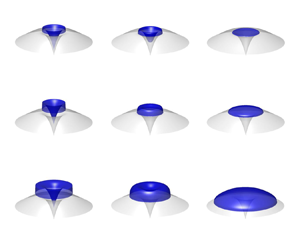
The axisymmetric propagation over the linear–exponential surface follows the same mechanism as two-dimensional propagation, due to the shared principles governing both cases. Figure 8 shows the evolution of the axisymmetric propagation as the released volume increases. When the released volume is smaller than the central cavity, the viscous fluid converges towards the centre, forming a horizontal plane without overflowing the peak. As the volume increases, the fluid surpasses the annular peak and begins to flow downward, gradually spreading across the entire linear–exponential surface. With further volume increases, part of the fluid remains trapped in the central cavity, while the rest continues to flow downward, eventually reaching the nearly horizontal section of the surface.
Temporal evolution of a viscous fluid over an axisymmetric linear–exponential surface under different release volumes for  $M = 0.08$ (a),
 $0.12$ (b),
 $0.8$ (c).

In axisymmetric propagation, viscous fluids typically remain laminar at low Reynolds numbers. However, as the fluid flows over a curvilinear surface, instabilities may develop, leading to phenomena such as flow separations and finger-like patterns. These instabilities result from the combined effects of gravity, viscous forces, inertial forces and surface tension. An increase in flow velocity or surface curvature, or a decrease in fluid viscosity, can cause the liquid film to thin, transitioning the flow from steady to unsteady. Furthermore, rough or abruptly changing surface curvatures can introduce additional perturbations, further amplifying flow instability.
4.2. Sinusoidal surface
We have examined the current evolution over linear–exponential surfaces, discussing typical cases based on the relationship between the initial condition of the released viscous fluid and the peak location. In this section, we shift our focus from the local issue of whether the released fluid can bypass the peak to a broader emphasis on global propagation. We extend our study to the propagation over sinusoidal surfaces.
Figure 9 illustrates the evolution of viscous gravity currents over a two-dimensional sinusoidal surface with two released volumes. At  $M=2{\rm \pi}$, as time progresses, the released fluid begins to simultaneously fill both sides of the adjacent troughs. For an initial length of
 $X_{0}=1.5{\rm \pi}$, most of the fluid accumulates in the left trough, resulting in a noticeable difference in the horizontal free surface levels between the left and right troughs. This indicates that for smaller released volumes, there may be an imbalance in fluid distribution between adjacent troughs. When the initial length increases to
 $X_{0}=2.5{\rm \pi}$, the horizontal free surfaces in both troughs gradually become more uniform. As the released volume increases to
 $M=6{\rm \pi}$, the viscous fluid fully fills the first two troughs, and the remaining fluid flows into the third trough. At this stage, the influence of the initial shape is no longer significant, as evidenced by the similar current profiles across all troughs.
Temporal evolution of a viscous fluid over a two-dimensional sinusoidal surface under different release volumes and initial lengths. Panels show (a)  $M = 2{\rm \pi}$,
 $X_{0} = 1.5{\rm \pi}$; (b)
 $M = 2{\rm \pi}$,
 $X_{0} = 2.5{\rm \pi}$; (c)
 $M = 6{\rm \pi}$,
 $X_{0} = 1.5{\rm \pi}$; (d)
 $M = 6{\rm \pi}$,
 $X_{0} = 2.5{\rm \pi}$.

Figure 10 provides a quantitative comparison of  $X_{F}$ and
 $H_{X=0}$ between sinusoidal and horizontal straight surfaces. At
 $M=2{\rm \pi}$, a clear difference in the evolution of
 $X_{F}$ emerges between the two surfaces. Over the horizontal straight surface,
 $X_{F}$ increases rapidly and consistently, displaying a monotonic growth. In contrast, over the sinusoidal surface,
 $X_{F}$ quickly reaches a steady state for all three initial lengths, as the second peak of the sinusoidal surface acts as a barrier that hinders further propagation of the fluid.
Comparison of the current front and height at the origin between a horizontal straight surface and a two-dimensional sinusoidal surface under different release volumes and initial lengths. Panels show (a,c)  $M = 2{\rm \pi}$; (b,d)
 $M = 6{\rm \pi}$; solid line, sinusoidal surface; dashed line, horizontal straight surface.

As the released volume increases to  $M=6{\rm \pi}$,
 $X_{F}$ rises significantly on both surfaces. Notably, during the early stages of propagation, the fluid over the sinusoidal surface may briefly advance further than on the horizontal surface, especially when the initial length begins on a downslope. However, as the fluid progresses upslope, its propagation inevitably decelerates. Without a pressure source at the bottom of the trough, the fluid must first fill the preceding trough entirely before it can pass the peak and flow into the next trough. This results in a non-monotonic
 $X_{F}$ trend over the sinusoidal surface, where the front alternates between slower upslope movement and faster downslope movement, eventually becoming confined by the troughs. For
 $H_{X=0}$ at
 $M=2{\rm \pi}$, the trend resembles that of case 1 over the linear–exponential surface, where the limited fluid volume primarily fills the left-hand space. At
 $M=6{\rm \pi}$, however, the fluid rapidly accumulates on the left, causing the liquid depth to increase before gradually decreasing as the fluid propagates to the right, following a pattern similar to that observed in cases 2 and 3.
Figure 11 illustrates the axisymmetric propagation of viscous gravity currents over a sinusoidal surface. As the released volume expands outward from the centre over time, the propagation is initially rapid, particularly between  $T = 0$ and
 $T = 5$. For a smaller released volume (
 $M = 155$), the expansion rate decreases significantly after the initial phase, whereas for a larger released volume (
 $M = 465$), the fluid continues to propagate outward. The behaviour of axisymmetric propagation closely parallels that observed in two-dimensional propagation, displaying similar stages of rapid initial spread followed by gradual deceleration.
Temporal evolution of a viscous fluid over an axisymmetric sinusoidal surface under different release volumes for  $M = 155$ (a),
 $465$ (b).

5. Computational fluid dynamics validation
We validate the low-dimensional models by comparing their predictions of the current profile and front with CFD simulations conducted using the open-source software OpenFOAM $^{\circledR }$. For two-dimensional propagation, we design a numerical domain where the top and right boundaries are set to atmospheric pressure, the left boundary is symmetric and the bottom boundary is no-slip. The mesh near the bottom boundary is refined to capture viscous dissipation in the boundary layer. For axisymmetric propagation, the three-dimensional domain is simplified into a two-dimensional profile to reduce computational costs. Glycerol (
 $\mu = 1.5$ Pa s;
 $\rho = 1.26\times 10^{3}$ kg m
 $^{-3}$;
 $\sigma = 0.063$ N m
 $^{-1}$) is used as the viscous fluid, initially placed in a square and cylinder with the remaining space filled with air. Upon release, the glycerol propagates gradually as a viscous gravity current over a curvilinear surface.
We test four different initial conditions: three for a linear–exponential surface (cases 1, 2 and 3) and one for a sinusoidal surface. Table 1 lists the surface parameters and the released volumes of glycerol. The Reynolds number is a key criterion for a viscous gravity current. The initial Reynolds number is defined as  $Re= Uh_{0}/\nu$, where the characteristic velocity is
 $U= \beta h_{0}^{3}/x_{0}$ (Ungarish Reference Ungarish2020). Based on this definition, the initial Reynolds numbers for the test cases are 1.13, 0.72, 0.45 and 21.78, respectively, placing them within the viscous–buoyancy regime.
Parameter of curvilinear surfaces in CFD simulations.

Figures 12 and 13 show a qualitative comparison between the numerical solutions and CFD results for current profiles at  $t = 1$ s in two-dimensional and axisymmetric propagation over curvilinear surfaces. In each case, the numerical solutions and CFD results visually align well. Typical flow patterns predicted by the numerical solutions, such as a horizontal free surface in case 1, slight overshooting of the peak in case 2, downslope flow in case 3 and traversal of two peaks on the sinusoidal surface, are all confirmed by CFD results.
Qualitative comparison between the numerical solutions of low-dimensional models and CFD results for two-dimensional propagation over linear–exponential and sinusoidal surfaces ( $t = 1$ s).

Qualitative comparison between the numerical solutions of low-dimensional models and CFD results for axisymmetric propagation over linear–exponential and sinusoidal surfaces ( $t = 1$ s).

Figure 14 presents the quantitative validation of the current front. In terms of  $X_{F}$, the numerical solutions and CFD results show excellent agreement in each case, although the numerical solutions slightly overestimate current propagation, a trend also observed in studies of horizontal straight surfaces (see Appendix A). This discrepancy is attributed to the full accounting of viscous dissipation and capillary effects in the CFD results. In conclusion, the above qualitative and quantitative comparisons validate the low-dimensional models for predicting the evolution of viscous gravity currents over curvilinear surfaces.
Quantitative CFD validation of current fronts for both propagation over linear–exponential and sinusoidal surfaces. Solid curve, numerical solution; symbols, CFD result.

6. Summary
In this study, we have focused on the evolution of a finite volume of viscous fluid at low Reynolds number over rigid curvilinear surfaces. To characterize the curvilinear surfaces, we consider linear–exponential and sinusoidal shapes, with single and multiple peaks, respectively. Based on lubrication theory, we establish approximate low-dimensional models and validate them with CFD simulation using the VOF method.
We reveal a significant dimensionless parameter  $M$ that governs the flow system. The physical interpretation of
 $M$ is straightforward, representing the volume ratio between the released viscous fluid and the curvilinear surface, so reflecting the interaction between them. When
 $M$ is small, it is difficult for the released viscous fluid to bypass the peaks on linear–exponential or sinusoidal surfaces, resulting in a constrained horizontal free surface. As
 $M$ increases, the fluid can bypass the peaks and flow downslope on linear–exponential surfaces or encounter subsequent peaks on sinusoidal surfaces. It is expected that, when
 $M$ is sufficiently large while
 $H_{0} \gg F(X)_{max}$, the effect from the curvilinear surface will become negligible, making fluid propagation quite similar to the performance over horizontal straight surfaces.
Further extending the curvilinear surfaces to more generalized power–exponential surfaces (see Appendix B) or arbitrary continuous surfaces by an expansion or transformation of the Fourier series (see Appendix C), the dimensionless number  $M$ still holds and the shape parameters of curvilinear surfaces will jointly govern the flow system.
Acknowledgements
We are thankful to Professor H.A. Stone for his, as usual, knowledgeable help in this study, as well as Professor M. Ungarish for his valuable and insightful suggestions. X.D. acknowledges the helpful discussions with Professor Z. Wang and the International Cooperation Program from Dalian University of Technology.
Declaration of interests
The authors report no conflict of interest.
Appendix A. Viscous gravity currents over horizontal straight surfaces
A.1. Two-dimensional propagation
The effectiveness of the numerical solution and CFD simulation are first validated by the classical similarity solutions for viscous gravity currents over horizontal straight surfaces. For two-dimensional propagation, the numerical solution can be obtained from the following low-dimensional model (Smith Reference Smith1969; Huppert Reference Huppert1982):
 \begin{equation} \frac{\partial h}{\partial t}-\beta\frac{\partial}{\partial x} \left(h^{3}\frac{\partial h}{\partial x}\right)=0. \end{equation}
For CFD simulation, we numerically simulate the propagation of glycerol in a two-dimensional domain with an initial volume of  $5\ {\rm cm}\times 1\ {\rm cm}$, corresponding to an initial Reynolds number of 1.36.
Figure 15 shows a visual comparison of the current profile. In (a), it can be observed that the numerical solution agrees very well with the similarity solution, although slightly overestimates the current propagation. This overestimation is consistent with previous findings, which suggest that in the early-time stage, the numerical solution takes time to converge to the similarity solution, gradually removing the effect of the initial shape of the released viscous fluid (Ball & Huppert Reference Ball and Huppert2019). In contrast, (b) reveals that the CFD result predicts shorter propagation. Unlike the low-dimensional model, which predicts a singularity at the current tip with the form  $h \sim (x_{f}-x)^{1/3}$ (Huppert Reference Huppert1982; Ungarish Reference Ungarish2020), the current tip in the CFD result appears crooked due to the capillary effects, allowing the moving contact angle between the tip and the bottom surface to be reproduced.
Comparison of current profile for two-dimensional propagation over a horizontal straight surface ( $t = 1$ s). (a) Similarity and numerical solutions; (b) CFD results.

Figure 16 displays the comparison of the current front, confirmed by mesh-independent tests with three different mesh numbers, denoted by  $N$. The difference between the CFD results and the similarity solution can be attributed to viscous dissipation during vertical deformation and within the boundary layer. Additionally, capillary effects may limit the current propagation and reduce the measured position of the front. These influencing factors are not accounted for in the low-dimensional model but fully captured by the Navier–Stokes equations-based VOF method.
Validation of current front for two-dimensional propagation over a horizontal straight surface.

A.2. Axisymmetric propagation
We next examine the axisymmetric propagation over horizontal straight surfaces, for which the low-dimensional model is given by (Huppert Reference Huppert1982)
 \begin{equation} \frac{\partial h}{\partial t}-\beta\frac{1}{r}\frac{\partial}{\partial r} \left(rh^{3}\frac{\partial h}{\partial r}\right)=0. \end{equation}
For CFD simulations, they are conducted within this two-dimensional profile of the three-dimensional cylindrical domain ( $h_{0}= 0.05$ m;
 $r_{0}= 0.01$ m). Figures 17 and 18 compare the current profile and front between the similarity solution, numerical solutions and CFD results, showing that all three exhibit similar behaviour to that observed in two-dimensional propagation. Therefore, this demonstrates the effectiveness of both the numerical solution and CFD simulation in studying viscous gravity currents, suggesting their suitabilities for numerical investigations of curvilinear surfaces.
Comparison of current profile for axisymmetric propagation over a horizontal straight surface ( $t = 1$ s). (a) Similarity and numerical solutions; (b) CFD results.

Validation of current front for axisymmetric propagation over a horizontal straight surface.

Appendix B. Two-dimensional generalized power–exponential surfaces
We further define the generalized two-dimensional power–exponential surface as
 \begin{equation} f(x)=ax^m\exp({-bx^n}), \end{equation}
where the parameters  $m$ (
 $m>1$) and
 $n$ (
 $n>1$) determine the single-peak shape of a power–exponential surface.
Using the following scalings,
 \begin{equation} S_{x}=(1/b)^{1/n},\quad S_{h}=a(S_{x})^m,\quad S_{t}=(S_{x})^{2-3m} /(\beta a^{3}), \end{equation}
we defined the generalized non-dimensional model
 $$\begin{gather} \frac{\partial H}{\partial T}-\frac{\partial}{\partial X} \left[H^{3}\left(\frac{\partial H}{\partial X}+\frac{{\rm d} F}{{\rm d}\kern0.06em X}\right)\right]=0, \end{gather}$$
 $$\begin{gather}\int_{0}^{L}H\,{\rm d}\kern0.06em X=M, \end{gather}$$
 $$\begin{gather}\left.\left(\frac{\partial H}{\partial X}+\frac{{\rm d} F}{{\rm d}\kern0.06em X}\right)\right|_{X=0}=0, \end{gather}$$
 $$\begin{gather}H(L,T)=0, \end{gather}$$
 $$\begin{gather}H(X,0)=\begin{cases} H_{0} &0\leq X\leq X_{0} \\ 0 & X>X_{0}, \end{cases} \end{gather}$$
 $$\begin{gather}X_{0}=M/H_{0}. \end{gather}$$
The above model keeps the same form as for previous linear–exponential surfaces. In this generalized case, the non-dimensional form of the power–exponential surface is written as
 \begin{equation} F(X)=X^m\,{\rm e}^{-X^n}, \end{equation}
and the definition of  $M$ is
 \begin{equation} M=\frac{q}{ab^{-(m+1)/n}}. \end{equation}
Because the two-dimensional volume of the generalized power–exponential surface,  $A_{ge}$, is calculated as
 \begin{equation} A_{ge}=\int_{0}^{+\infty}ax^m\exp({-bx^n})\,{{\rm d}\kern0.06em x}=\frac{a}{nb^{(m+1)/n}}\varGamma((m+1)/n), \end{equation}
it follows that
 \begin{equation} M=\frac{\varGamma((m+1)/n)}{n}\frac{q}{A_{ge}}. \end{equation}
This result suggests that when a finite-volume viscous fluid is released over an arbitrary power–exponential surface, the dimensionless parameter  $M$ consistently governs the flow system. Both
 $M$ and
 $F(X)$ reflect the influence of shape parameters on current evolution.
Appendix C. Two-dimensional arbitrary continuous surfaces
We extend the sinusoidal surface to arbitrary continuous surfaces. For simplicity, we define a curvilinear surface consisting of the following components:
 \begin{equation} f(x)=\sum_{i=1}^{N} A_{i}[1-\cos(\lambda_{i} x)]. \end{equation}
Letting  $N=3$, the curvilinear surface can be expressed as
 \begin{equation} f(x)=A_{1}[1-\cos(\lambda_{1} x)]+ A_{2}[1-\cos(\lambda_{2} x)]+ A_{3}[1-\cos(\lambda_{3} x)]. \end{equation}
Therein, the first term,  $A_{1}[1-\cos (\lambda _{1} x)]$, is the primary term, and the two subsequent secondary terms are the high-frequency terms, i.e.
 $\lambda _{3}>\lambda _{2}>\lambda _{1}$.
Using the following scalings,
 \begin{equation} S_{x}=1/\lambda_{1},\quad S_{h}=A_{1},\quad S_{t}=1/(\beta \lambda_{1}^{2}A_{1}^{3}), \end{equation}
the same generalized non-dimensional model is derived
 $$\begin{gather} \frac{\partial H}{\partial T}-\frac{\partial}{\partial X} \left[H^{3}\left(\frac{\partial H}{\partial X}+\frac{{\rm d} F}{{\rm d}\kern0.06em X}\right)\right]=0, \end{gather}$$
 $$\begin{gather}\int_{0}^{L}H\,{\rm d}\kern0.06em X=M, \end{gather}$$
 $$\begin{gather}\left.\left(\frac{\partial H}{\partial X}+\frac{{\rm d} F}{{\rm d}\kern0.06em X}\right)\right|_{X=0}=0, \end{gather}$$
 $$\begin{gather}H(L,T)=0, \end{gather}$$
 $$\begin{gather}H(X,0)=\begin{cases}
H_{0} & 0\leq X\leq X_{0}\\
0 & X>X_{0}, \end{cases}
\end{gather}$$
 $$\begin{gather}X_{0}=M/H_{0}, \end{gather}$$
and the non-dimensional form of this curvilinear surface is written as
 \begin{equation} F(X)=1-\cos(X)+P_{2}[1-\cos(Q_{2}X)]+P_{3}[1-\cos(Q_{3}X)], \end{equation}
where
 $$\begin{gather} P_{2}=A_{2}/A_{1},\quad Q_{2}=\lambda_{2}/\lambda_{1}, \end{gather}$$
 $$\begin{gather}P_{3}=A_{3}/A_{1},\quad Q_{3}=\lambda_{3}/\lambda_{1}, \end{gather}$$
i.e. the amplitude and the frequency ratios between the secondary terms to the primary term.
Here,  $M$ is defined as
 \begin{equation} M=2{\rm \pi} q/A_{s1}, \end{equation}
where  $A_{s1}$ is the two-dimensional volume of the primary term
 \begin{equation} A_{s1}=A_{1}\int_{0}^{2{\rm \pi}/\lambda_{1}}[1-\cos(\lambda_{1} x)]\,{{\rm d}\kern0.06em x}=2{\rm \pi} A_{1}/\lambda_{1}. \end{equation}
The above result suggests that, for an arbitrary continuous surface composed of multiple sinusoidal superpositions, the flow system is still governed by the dimensionless released volume  $M$. However, similar to generalized power–exponential surfaces, the shape parameters of the curvilinear surface,
 $F(X)$, such as
 $P_{i}$ and
 $Q_{i}$ in this case, also influence the flow system.


 Open access

