1 Introduction
The dynamics of fluid systems in rapid rotation are strongly influenced by the restorative nature of the Coriolis force, rendering the system to act like an oscillator. Systems slightly perturbed away from solid-body rotation (SBR) tend to return to SBR via viscous dissipation, but it is possible to maintain them away from SBR by continuously perturbing them. The situation becomes interesting when the deviation away from SBR is much larger than the size of the perturbation. For a simple oscillator, this happens when it is forced with small amplitude at the natural frequency. This idea provides a mechanism to extract energy from that available in the rapidly rotating flow to drive large-scale flows via small-amplitude mechanical forcing at or near-resonant frequencies. Furthermore, this idea has wide-ranging implications in rapidly rotating geophysical and astrophysical flows (Malkus Reference Malkus1968; Tilgner Reference Tilgner2005; Noir et al. Reference Noir, Hemmerlin, Wicht, Baca and Aurnou2009; Davidson Reference Davidson2013; Le Bars, Cebron & Le Gal Reference Le Bars, Cebron and Le Gal2015). For rapidly rotating fluid systems, much insight has been gained from linearizing the system about SBR and considering the response to various types of forced perturbations. Greenspan (Reference Greenspan1968) gives a comprehensive account of the early work in this regard, and in their review article, Le Bars et al. (Reference Le Bars, Cebron and Le Gal2015) give an overview of the more recent experimental, theoretical and numerical investigations of the flow response to various types of mechanical forcings, including libration, precession and tidal forcing.
The linear inviscid equations are of hyperbolic type when the disturbance frequency is less than twice the SBR frequency (Lord Kelvin Reference Kelvin1880). The inviscid inertial eigenmodes of the container, known as Kelvin modes when the container is a right-circular cylinder, have a particular spatial structure depending on the disturbance frequency. These are neutral modes, i.e. the real part of the eigenvalues is zero. In a viscous setting these modes are expected to be damped, and those with higher spatial variations more so (Greenspan Reference Greenspan1968, p. 83). So, in a rapidly rotating viscous flow, one expects to preferentially excite modes with low spatial variation via near-resonant forcing (Aldridge & Toomre Reference Aldridge and Toomre1969). The spatial structure of the imposed forcing may also play a role in selecting modes of similar structure. The experiments of Boisson et al. (Reference Boisson, Lamriben, Maas, Cortet and Moisy2012), consisting of a rapidly rotating fluid-filled cube subjected to small-amplitude libration over a range of frequencies, strongly suggest that the spatial structure of the forcing indeed influences the resonant response.
A further complication in all of this is that rapidly rotating flows that are subjected to localized perturbations with frequencies less than twice the SBR frequency emit inertial wave beams from the localized perturbation along the directions of the characteristics of the hyperbolic system. For the librating cube under consideration, the localized perturbations are at the edges where the top and bottom endwalls meet the vertical sidewalls and are driven by the Ekman fluxes in the top and bottom endwall boundary layers (Boisson et al. Reference Boisson, Lamriben, Maas, Cortet and Moisy2012); the vertical direction being taken in the direction of the mean rotation. The flow response can be dominated by the beams, completely swamping the contribution from the resonantly excited eigenmode. Which dominates, beam or eigenmode, is not straightforward to predict a priori, and it depends on how fast the system is rotating compared to how fast it viscously dissipates, and on how small the forcing amplitude is. The concepts of inviscid inertial eigenmodes and inertial wave beams stem from analysing the governing equations in two limits: inviscid (vanishing Ekman number) and linear (vanishing Rossby number). These limits present challenges to both experimental investigations and to numerical simulations of the Navier–Stokes equations.
Here we report on numerical simulations of the full three-dimensional Navier–Stokes equations with no-slip boundary conditions corresponding to the librating cube experiments of Boisson et al. (Reference Boisson, Lamriben, Maas, Cortet and Moisy2012). We reproduce their experimental findings and then consider a series of simulations in which both the Ekman number and the Rossby number are reduced significantly, and we also extend the range of libration frequencies considered to cover from zero to twice the SBR frequency. We find peak responses at many frequencies and are able to identify either low-order inertial inviscid eigenmodes or low-order retracing edge beams in these responses. If the Ekman number is too large, the contributions from these eigenmodes and retracing beams are blended due to viscous effects. The beams are present at all frequencies, and for moderate Ekman numbers their contribution to the response is essentially uniform in frequency, regardless of whether they retrace or not. Reducing the Ekman number increases the separation between the peaks by both sharpening the peaks and reducing detuning. Even for very small libration amplitudes (Rossby number), nonlinear effects are evident in the response, primarily consisting of the beams pinning and deforming the eigenmode spatio-temporal structure.
2 Governing equations and their symmetries
Consider a cube with sides of length
 $L$
, completely filled with an incompressible fluid of kinematic viscosity
 $\unicode[STIX]{x1D708}$
that has a mean rotation
 $\unicode[STIX]{x1D6FA}_{0}$
that is modulated harmonically at a frequency
 $\unicode[STIX]{x1D70E}_{0}$
and relative amplitude
 $\unicode[STIX]{x1D716}$
, which is often referred to as the Rossby number of the libration. The system is non-dimensionalized using
 $L$
as the length scale and
 $1/\unicode[STIX]{x1D6FA}_{0}$
as the time scale, and described in terms of a non-dimensional Cartesian coordinate system
 $\boldsymbol{x}=(x,y,z)$
that is fixed in the cube, with the origin at the centre of the cube and the rotation vector pointing in the
 $z$
direction (which we refer to as the vertical direction). The non-dimensional velocity field is
 $\boldsymbol{u}=(u,v,w)$
and the corresponding vorticity field is
 $\unicode[STIX]{x1D735}\times \boldsymbol{u}=(\unicode[STIX]{x1D714}_{x},\unicode[STIX]{x1D714}_{y},\unicode[STIX]{x1D714}_{z})$
. The non-dimensional angular velocity is
 $$\begin{eqnarray}\boldsymbol{\unicode[STIX]{x1D6FA}}(t)=[1+\unicode[STIX]{x1D716}\cos (2\unicode[STIX]{x1D714}t)]\boldsymbol{e}_{z},\end{eqnarray}$$
where the non-dimensional libration frequency
 $2\unicode[STIX]{x1D714}=\unicode[STIX]{x1D70E}_{0}/\unicode[STIX]{x1D6FA}_{0}$
, and
 $\boldsymbol{e}_{z}$
is the unit vector in the
 $z$
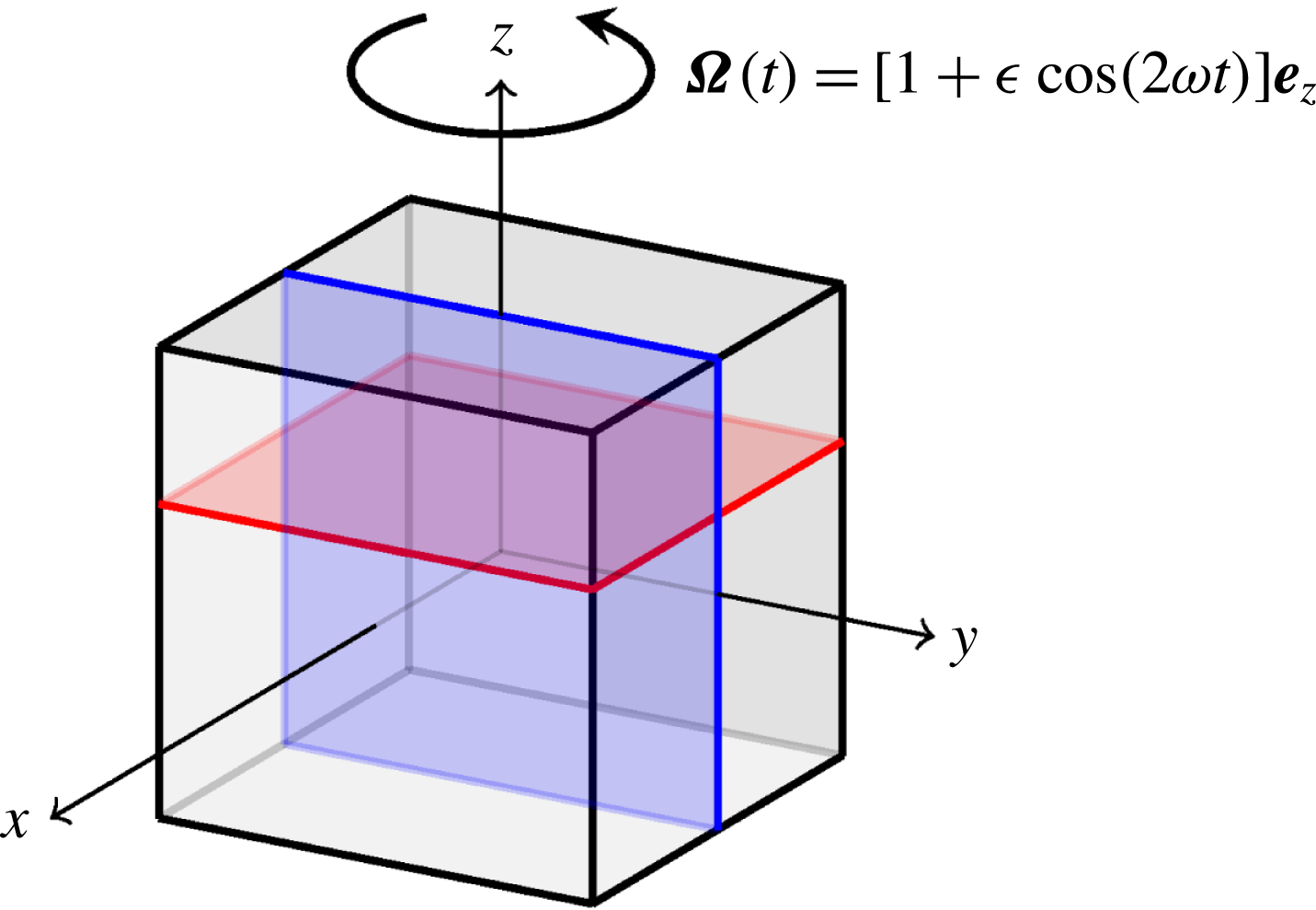
direction. Figure 1 shows a schematic of the system. Using a non-inertial frame of reference, the cube frame, introduces both a Coriolis and an Euler body force into the (non-dimensional) governing equations:
 $$\begin{eqnarray}\frac{\unicode[STIX]{x2202}\boldsymbol{u}}{\unicode[STIX]{x2202}t}+\boldsymbol{u}\boldsymbol{\cdot }\unicode[STIX]{x1D735}u+2\boldsymbol{\unicode[STIX]{x1D6FA}}\times \boldsymbol{u}+\frac{\text{d}\boldsymbol{\unicode[STIX]{x1D6FA}}}{\text{d}t}\times \boldsymbol{x}=-\unicode[STIX]{x1D735}p+\mathit{E}\unicode[STIX]{x1D6FB}^{2}\boldsymbol{u},\quad \unicode[STIX]{x1D735}\boldsymbol{\cdot }\boldsymbol{u}=0,\quad \boldsymbol{u}|_{\unicode[STIX]{x2202}{\mathcal{C}}}=\mathbf{0},\end{eqnarray}$$
where
 $\mathit{E}=\unicode[STIX]{x1D708}/\unicode[STIX]{x1D6FA}_{0}L^{2}$
is the Ekman number giving the ratio of the mean rotation time scale,
 $1/\unicode[STIX]{x1D6FA}_{0}$
, to the viscous time scale,
 $L^{2}/\unicode[STIX]{x1D708}$
. In the cube frame of reference, the no-slip boundary conditions on all six walls of the cube are trivial (
 $\unicode[STIX]{x2202}{\mathcal{C}}$
signifies the boundaries of the cube). Note that Boisson et al. (Reference Boisson, Lamriben, Maas, Cortet and Moisy2012) define the Ekman number as
 $\unicode[STIX]{x1D708}/[2\unicode[STIX]{x1D6FA}_{0}(L/2)^{2}]$
, where they used
 $L/2$
as the length scale and
 $1/2\unicode[STIX]{x1D6FA}_{0}$
as the time scale, so that their Ekman number is twice ours.
Schematic of the librating cube, including the observation planes
 $x=0$
(vertical) and
 $z=1/6$
(horizontal).

The Navier–Stokes system (2.2) is invariant to a reflection through the plane
 $z=0$
, and a
 $\unicode[STIX]{x03C0}/2$
rotation about the
 $z$
-axis. The actions of these symmetries on the velocity and pressure are
 $$\begin{eqnarray}\displaystyle \left.\begin{array}{@{}c@{}}{\mathcal{K}}_{z}(u,v,w,p)(x,y,z,t)=(u,v,-w,p)(x,y,-z,t),\\ {\mathcal{R}}_{\unicode[STIX]{x03C0}/2}(u,v,w,p)(x,y,z,t)=(-v,u,w,p)(-y,x,z,t).\end{array}\right\} & & \displaystyle\end{eqnarray}$$
These are the only spatial symmetries of the Navier–Stokes system (2.2).
The inviscid inertial modes are the eigensolutions to the inviscid limit of system (2.2), linearized about the state of solid-body rotation, i.e.
 $$\begin{eqnarray}\frac{\unicode[STIX]{x2202}\boldsymbol{u}}{\unicode[STIX]{x2202}t}+2\boldsymbol{\unicode[STIX]{x1D6FA}}_{0}\times \boldsymbol{u}=-\unicode[STIX]{x1D735}p,\quad \unicode[STIX]{x1D735}\boldsymbol{\cdot }\boldsymbol{u}=0,\quad \boldsymbol{u}\boldsymbol{\cdot }\boldsymbol{n}|_{\unicode[STIX]{x2202}{\mathcal{C}}}=0,\end{eqnarray}$$
where
 $\boldsymbol{n}$
is the normal at the walls of the cube and
 $\boldsymbol{\unicode[STIX]{x1D6FA}}_{0}=\boldsymbol{e}_{z}$
.
Since the linearized inviscid system (2.4) is a direct reduction from (2.2), it also is invariant to
 ${\mathcal{K}}_{z}$
and
 ${\mathcal{R}}_{\unicode[STIX]{x03C0}/2}$
. The system (2.4) is invariant to an additional spatial symmetry,
 $$\begin{eqnarray}\overline{{\mathcal{R}}}_{\unicode[STIX]{x03C0}/2}(u,v,w,p)(x,y,z,t)=(v,-u,-w,-p)(-y,x,z,t).\end{eqnarray}$$
Both the nonlinear term
 $\boldsymbol{u}\boldsymbol{\cdot }\unicode[STIX]{x1D735}u$
and the Euler force term
 $\text{d}\boldsymbol{\unicode[STIX]{x1D6FA}}/\text{d}t\times \boldsymbol{x}$
in (2.2) break
 $\overline{{\mathcal{R}}}_{\unicode[STIX]{x03C0}/2}$
. For small enough forcing
 $\unicode[STIX]{x1D716}$
, (2.2) has a unique solution which is invariant to all symmetries of the system (
 ${\mathcal{K}}_{z}$
and
 ${\mathcal{R}}_{\unicode[STIX]{x03C0}/2}$
) and is synchronous with the forcing. In
 $(\mathit{E},\unicode[STIX]{x1D716})$
-parameter space, there is a critical curve dividing the parameter space into regions where this symmetric synchronous state is stable and where it is not. The objective of the experiments in Boisson et al. (Reference Boisson, Lamriben, Maas, Cortet and Moisy2012) was to see what is the forced response for small
 $\mathit{E}$
and
 $\unicode[STIX]{x1D716}$
, and how the response is related to the eigenmodes of (2.4). A conclusion from their study was that only eigenmodes with the symmetry of the librational forcing could be excited. They reasoned that the modes with
 $\overline{{\mathcal{R}}}_{\unicode[STIX]{x03C0}/2}$
invariance could not be excited because the librational forcing does not have this symmetry.
Maas (Reference Maas2003) determined the eigenmodes of (2.4) using separation of variables, obtaining modes that are sinusoidal standing waves in
 $z$
with
 $n$
half-wavelengths, and harmonic in
 $t$
with (non-dimensional) frequency in the range
 $[0,1]$
. For each
 $n$
, the horizontal
 $(x,y)$
structure of the modes was expressed in terms of infinite sums of Fourier modes in
 $x$
and
 $y$
, and these were truncated in order to compute them. The finite number of resulting eigenfrequencies were enumerated by
 $m$
, with larger
 $m$
values loosely corresponding to smaller horizontal scales. Boisson et al. (Reference Boisson, Lamriben, Maas, Cortet and Moisy2012) noted that the eigenmodes are either invariant to
 ${\mathcal{R}}_{\unicode[STIX]{x03C0}}={\mathcal{R}}_{\unicode[STIX]{x03C0}/2}\circ {\mathcal{R}}_{\unicode[STIX]{x03C0}/2}$
or to
 $\overline{{\mathcal{R}}}_{\unicode[STIX]{x03C0}}=\overline{{\mathcal{R}}}_{\unicode[STIX]{x03C0}/2}\circ \overline{{\mathcal{R}}}_{\unicode[STIX]{x03C0}/2}$
. This led to naming the modes
 $[n,m,s]$
, where
 $s=+$
for the
 ${\mathcal{R}}_{\unicode[STIX]{x03C0}}$
-symmetric modes and
 $s=-$
for the
 $\overline{{\mathcal{R}}}_{\unicode[STIX]{x03C0}}$
-symmetric modes. They then asserted that libration of the cube is expected to excite only a subset of the modes
 $[n,m,s]$
, namely those with
 $n$
even and
 $s=+$
; this being due to the top and bottom endwall velocities being the same implying
 $n$
even, and that these velocity boundary conditions are invariant to
 ${\mathcal{R}}_{\unicode[STIX]{x03C0}}$
, implying
 $s=+$
. Certainly, in their experiments these are the only types of modes that they observed. At the very end of section V, they state that only modes that are also invariant to
 ${\mathcal{R}}_{\unicode[STIX]{x03C0}/2}$
can be excited. Their assertions are correct, basically reducing to the fact that the unique response at small enough
 $\unicode[STIX]{x1D716}$
for a given
 $\mathit{E}$
is synchronous,
 ${\mathcal{K}}_{z}$
invariant (
 $n$
even), and
 ${\mathcal{R}}_{\unicode[STIX]{x03C0}/2}$
invariant, i.e. has all the symmetries of (2.2). In light of this, here we only consider modes with all the symmetries of (2.2), and use the simpler notation
 $M_{n.m}$
for these
 ${\mathcal{K}}_{z}\times {\mathcal{R}}_{\unicode[STIX]{x03C0}/2}$
-symmetric modes with
 $n$
half-wavelengths in
 $z$
and
 $m$
th largest frequency. The computation of those modes as well as the correspondence between the
 $M_{n.m}$
notation used here and the
 $[n,m,+]$
notation used in Boisson et al. (Reference Boisson, Lamriben, Maas, Cortet and Moisy2012) is described in appendix A. In both notations
 $n$
corresponds to the half wavenumber in the vertical direction, while
 $m$
indexes the modes according to their frequencies. However, the values of
 $m$
associated with a specific mode do not necessarily correspond between the two notations (
 $[n,m,+]$
include both
 ${\mathcal{R}}_{\unicode[STIX]{x03C0}/2}$
and
 $\overline{{\mathcal{R}}}_{\unicode[STIX]{x03C0}/2}$
invariant modes, whereas
 $M_{n.m}$
denote only the
 ${\mathcal{R}}_{\unicode[STIX]{x03C0}/2}$
invariant modes).
3 Numerical technique for the viscous nonlinear forced flow
The Navier–Stokes system (2.2) is discretized using a spectral-collocation method in all three spatial directions. The velocity and pressure are approximated by polynomials of degree
 $N$
written in barycentric form with weights
 $w_{0}=0.5$
,
 $w_{n}=(-1)^{n}$
for
 $n\in [1,N-1]$
, and
 $w_{N}=0.5(-1)^{N}$
, associated with the Chebyshev–Gauss–Lobatto grid. Spatial differentiation is performed via direct matrix–vector multiplication by the pseudospectral differentiation matrix (common to all three directions).
The time integration scheme used is the fractional-step improved projection method of Hugues & Randriamampianina (Reference Hugues and Randriamampianina1998), based on a linearly implicit and stiffly stable, second-order accurate scheme combining a backward differentiation formula for the linear terms and an explicit mix, equivalent to linear extrapolation, of Adams–Moulton and Adams–Bashforth steps for the nonlinear convective terms (Vanel, Peyret & Bontoux Reference Vanel, Peyret, Bontoux, Morton and Baines1986). The predictor stage of the fractional-step method solves a Helmholtz equation for a pressure field, for which Neumann conditions consistent with (2.2) are applied at the walls. The corrector stage then projects the resulting predicted velocity field onto the space of (discretely) divergence-free polynomials via a Stokes problem, which is also handled by solving a Helmholtz equation for the corrected pressure, albeit with homogeneous Neumann boundary conditions. Further details can be found in Hugues & Randriamampianina (Reference Hugues and Randriamampianina1998).
The code was verified and validated against the experimental results of Boisson et al. (Reference Boisson, Lamriben, Maas, Cortet and Moisy2012), most of which are reproduced numerically in the following section. The Ekman number
 $\mathit{E}$
determines the thickness of the boundary layers and edge beams in the interior, and these are the features that need to be resolved numerically. The boundary layer thickness scales with
 $\mathit{E}^{1/2}$
, it is the thinnest length scale in the problem, and the edge beam thickness scales with
 $\mathit{E}^{1/3}$
(Wood Reference Wood1966). The Chebyshev–Gauss–Lobatto collocation grid distribution leads to very well resolved boundary layers. For small libration amplitudes (
 $\unicode[STIX]{x1D716}<0.1$
),
 $\unicode[STIX]{x1D716}$
does not add any further constraints on the spatial (or temporal) resolution requirements. In this study, we report on results for Ekman numbers in the range
 $\mathit{E}\in [10^{-6},10^{-4.6}]$
(the larger value corresponding to the experimental condition used by Boisson et al. (Reference Boisson, Lamriben, Maas, Cortet and Moisy2012)), for which we used different spatial resolutions. We used
 $N^{3}=72^{3}$
collocation points for
 $\mathit{E}\geqslant 10^{-5}$
,
 $N^{3}=96^{3}$
for
 $\mathit{E}=10^{-5.5}$
, and
 $N^{3}=156^{3}$
for
 $\mathit{E}=10^{-6}$
. With these grid resolutions, the solutions manifest spectral convergence of at least six orders of magnitude. The required temporal resolution depends on the libration frequency
 $2\unicode[STIX]{x1D714}$
. For
 $\unicode[STIX]{x1D714}\in [0.58,1)$
, we used 100 time steps per libration period
 $\unicode[STIX]{x1D70F}=\unicode[STIX]{x03C0}/2\unicode[STIX]{x1D714}$
so that the time step
 $\unicode[STIX]{x1D6FF}t=\unicode[STIX]{x1D70F}/100$
. For the lower frequencies,
 $\unicode[STIX]{x1D714}<10^{.58}$
, we used
 $80/\unicode[STIX]{x1D714}$
(rounded up to the nearest integer) time steps per period. Being a forced oscillator problem, the response consists of a transient and a forced response. In order to examine the forced response, the system needs to be integrated in time until the transient contribution is negligible. As
 $\mathit{E}$
is reduced, the transient is longer lived. For
 $\mathit{E}=10^{-6}$
, we find that this occurs in a few multiples of the spin-up time
 $\mathit{E}^{-1/2}$
, which is much shorter than the viscous time
 $\mathit{E}^{-1}$
. For small libration amplitudes
 $\unicode[STIX]{x1D716}$
, the response is the unique synchronous symmetric basic state, and as such it is computed independent of initial conditions.
Since the flows being studied are
 ${\mathcal{K}}_{z}$
invariant, the volume integrals of the velocity
 $\boldsymbol{u}$
and helicity
 $\mathit{H}=\boldsymbol{u}\boldsymbol{\cdot }(\unicode[STIX]{x1D735}\times \boldsymbol{u})$
both vanish, but their variances do not. Convenient global measures of the forced response are the time averages of the standard deviations away from solid-body rotation in the velocity,
 $\unicode[STIX]{x1D6F4}_{V}$
, and the helicity,
 $\unicode[STIX]{x1D6F4}_{H}$
, relative to the amplitude of the libration
 $\unicode[STIX]{x1D716}$
, where
 $$\begin{eqnarray}\unicode[STIX]{x1D6F4}_{V}^{2}=\frac{1}{\unicode[STIX]{x1D70F}\unicode[STIX]{x1D716}^{2}}\int _{0}^{\unicode[STIX]{x1D70F}}\int _{{\mathcal{V}}}|\boldsymbol{u}|^{2}\,\text{d}{\mathcal{V}}\,\text{d}t\quad \text{and}\quad \unicode[STIX]{x1D6F4}_{H}^{2}=\frac{1}{\unicode[STIX]{x1D70F}\unicode[STIX]{x1D716}^{4}}\int _{0}^{\unicode[STIX]{x1D70F}}\int _{{\mathcal{V}}}|\boldsymbol{u}\boldsymbol{\cdot }(\unicode[STIX]{x1D735}\times \boldsymbol{u})|^{2}\;\text{d}{\mathcal{V}}\;\text{d}t.\end{eqnarray}$$
The volume integrals are computed over a volume
 ${\mathcal{V}}$
which excludes the boundary layers. The thickness of the boundary layers was determined from
 $z$
-profiles of the
 $\unicode[STIX]{x1D714}_{x}$
vorticity component (similar to the approach in Lopez & Marques Reference Lopez and Marques2014; Gutierrez-Castillo & Lopez Reference Gutierrez-Castillo and Lopez2017). As expected, the thickness varies with
 $\mathit{E}^{1/2}$
. Also note that
 $0.5\unicode[STIX]{x1D716}^{2}\unicode[STIX]{x1D6F4}_{V}^{2}$
is the time average of the kinetic energy in
 ${\mathcal{V}}$
.
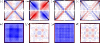
Contours of
 $\unicode[STIX]{x1D714}_{x}$
in the vertical plane
 $x=0$
for
 $\unicode[STIX]{x1D714}=0.6742$
at phases
 $\unicode[STIX]{x1D711}=2\unicode[STIX]{x1D714}t\hspace{0.6em}{\rm mod}\hspace{0.2em}2\unicode[STIX]{x03C0}$
of the oscillation (a)
 $\unicode[STIX]{x1D711}=0$
and (b)
 $\unicode[STIX]{x1D711}=\unicode[STIX]{x03C0}/2$
, and for
 $\unicode[STIX]{x1D714}=0.6484$
at phases (c)
 $\unicode[STIX]{x1D711}=0$
and (d)
 $\unicode[STIX]{x1D711}=\unicode[STIX]{x03C0}/2$
, and of
 $\unicode[STIX]{x1D714}_{z}$
in the horizontal plane
 $z=1/6$
for
 $\unicode[STIX]{x1D714}=0.6742$
at phases (e)
 $\unicode[STIX]{x1D711}=0$
and (f)
 $\unicode[STIX]{x1D711}=\unicode[STIX]{x03C0}/2$
, and for
 $\unicode[STIX]{x1D714}=0.6484$
at phases (g)
 $\unicode[STIX]{x1D711}=0$
and (h)
 $\unicode[STIX]{x1D711}=\unicode[STIX]{x03C0}/2$
, all for
 $(\mathit{E},\unicode[STIX]{x1D716})=(10^{-4.6},0.04)$
corresponding to the two experimental cases in figures 5 and 6 of Boisson et al. (Reference Boisson, Lamriben, Maas, Cortet and Moisy2012). Contour levels are equispaced
 $|\unicode[STIX]{x1D714}_{x}|\leqslant 3000$
and
 $|\unicode[STIX]{x1D714}_{z}|\leqslant 5000$
. See the online movie 1 for animations over one libration period.

4 Results
We begin by simulating two cases that were investigated in detail in the experiments of Boisson et al. (Reference Boisson, Lamriben, Maas, Cortet and Moisy2012). These cases were at (half) libration frequencies
 $\unicode[STIX]{x1D714}=0.6742$
and
 $0.6484$
, both with
 $\mathit{E}=2.65\times 10^{-5}\approx 10^{-4.6}$
and
 $\unicode[STIX]{x1D716}=0.04\approx 10^{-1.4}$
. These two frequencies were selected because they correspond to the lowest-order eigenmodes with
 $n=2$
(a full sine wavelength in
 $z$
) that are
 ${\mathcal{R}}_{\unicode[STIX]{x03C0}}$
invariant (
 $s=+$
), and they are the leading two such modes:
 $[2,1,+]$
(
 $M_{2.1}$
in our notation) for
 $\unicode[STIX]{x1D714}=0.6742$
, and
 $[2,2,+]$
(which is
 $\overline{{\mathcal{R}}}_{\unicode[STIX]{x03C0}/2}$
invariant but not
 ${\mathcal{R}}_{\unicode[STIX]{x03C0}/2}$
invariant) for
 $\unicode[STIX]{x1D714}=0.6484$
. Figures 2(a–d) show the horizontal vorticity
 $\unicode[STIX]{x1D714}_{x}$
in the plane
 $x=0$
at phases
 $\unicode[STIX]{x1D711}=2\unicode[STIX]{x1D714}t\hspace{0.6em}{\rm mod}\hspace{0.2em}2\unicode[STIX]{x03C0}=0$
and
 $\unicode[STIX]{x03C0}/2$
, and figures 2(e–h) show the vertical vorticity
 $\unicode[STIX]{x1D714}_{z}$
in the plane
 $z=1/6$
, also at phases
 $\unicode[STIX]{x1D711}=0$
and
 $\unicode[STIX]{x03C0}/2$
. These can be compared directly with the experimental results in the same planes and phases in figures 5 and 6 of Boisson et al. (Reference Boisson, Lamriben, Maas, Cortet and Moisy2012). Furthermore, the online movie 1 available at https://doi.org/10.1017/jfm.2018.157, of our simulations, can also be directly compared with the corresponding movies of the experimental results which Boisson et al. (Reference Boisson, Lamriben, Maas, Cortet and Moisy2012) make available as online supplementary material, showing animations over a libration period. There is excellent agreement between our numerical simulations and the experimental measurements. As noted by Boisson et al. (Reference Boisson, Lamriben, Maas, Cortet and Moisy2012), the
 $\unicode[STIX]{x1D714}=0.6742$
case shows the structure of the eigenmode
 $[2,1,+]$
(
 $M_{2.1}$
), particularly during phases of the libration period where the edge beams are weakest, but the
 $\unicode[STIX]{x1D714}=0.6484$
case does not have the horizontal structure of the
 $[2,2,+]$
eigenmode, which is
 $\overline{{\mathcal{R}}}_{\unicode[STIX]{x03C0}/2}$
invariant but not
 ${\mathcal{R}}_{\unicode[STIX]{x03C0}/2}$
invariant. It is clear from figures 2
 $(g,h)$
that the response at
 $\unicode[STIX]{x1D714}=0.6484$
is
 ${\mathcal{R}}_{\unicode[STIX]{x03C0}/2}$
invariant.
For the same two (half) libration frequencies,
 $\unicode[STIX]{x1D714}=0.6742$
and
 $\unicode[STIX]{x1D714}=0.6484$
, we varied
 $\unicode[STIX]{x1D716}$
from
 $0.02$
to
 $0.16$
, as was done in Boisson et al. (Reference Boisson, Lamriben, Maas, Cortet and Moisy2012) to show that the kinetic energy of the response (measured in the plane
 $z=1/6$
) scales with
 $\unicode[STIX]{x1D716}^{2}$
. We have verified this, and hence defined
 $\unicode[STIX]{x1D6F4}_{V}^{2}$
in (3.1) with an
 $\unicode[STIX]{x1D716}^{-2}$
factor and
 $\unicode[STIX]{x1D6F4}_{H}^{2}$
with an
 $\unicode[STIX]{x1D716}^{-4}$
factor.
Boisson et al. (Reference Boisson, Lamriben, Maas, Cortet and Moisy2012) studied the system response to different librational frequencies in the range
 $\unicode[STIX]{x1D714}\in [0.60,0.73]$
, for
 $\mathit{E}=2.65\times 10^{-5}$
and
 $\unicode[STIX]{x1D716}=0.02$
. Note that over this range of
 $\unicode[STIX]{x1D714}$
, the linear dispersion relation dictates that the edge beams are inclined with respect to the
 $(x,y)$
-plane at angles ranging from
 $\arccos (0.60)\approx 53.13^{\circ }$
to
 $\arccos (0.73)\approx 43.11^{\circ }$
. To quantify the response, they used particle image velocimetry (PIV) measurements of the velocity in the vertical plane
 $x=0$
(excluding the boundary region 8 % in from the walls as the PIV measurements there were unreliable) to calculate the corresponding
 ${\mathcal{L}}_{2}$
norm of the kinetic energy associated with the velocity components in that measurement plane, scaled by
 $\unicode[STIX]{x1D716}^{-2}$
. Their results (figure 8 in their paper) showed a well-defined peak at
 $\unicode[STIX]{x1D714}\approx 0.676$
, which they associated with the
 $[2,1,+]$
mode (
 $M_{2.1}$
in our notation), which is
 ${\mathcal{K}}_{z}\times {\mathcal{R}}_{\unicode[STIX]{x03C0}/2}$
invariant. Surrounding this peak, the response is nearly constant at approximately 15 % of the peak response, which they interpreted as being associated with the kinetic energy of the edge beams. They also noted the presence of a slight bump in the response at
 $\unicode[STIX]{x1D714}\approx 0.695$
, and suggested that this could be attributed to the
 $[4,5,+]$
mode (
 $M_{4.3}$
), which has an eigenfrequency
 $\unicode[STIX]{x1D70E}\approx 0.6962$
and is also
 ${\mathcal{K}}_{z}\times {\mathcal{R}}_{\unicode[STIX]{x03C0}/2}$
invariant. They did not report any clear evidence of any other eigenmodes being excited.
Boisson et al. (Reference Boisson, Lamriben, Maas, Cortet and Moisy2012) also tried to find some relationship between the low-order inviscid inertial modes (i.e.
 $[n,m,+]$
with
 $n$
even and both
 $n$
and
 $m$
small) and the low-order retracing rays. The ray tracing concept relates to the characteristics of the linear inviscid system (2.4). The characteristics are aligned with respect to the mean rotation axis according to the linear dispersion relation; for a disturbance frequency
 $\unicode[STIX]{x1D714}$
, characteristics are inclined at angle
 $\unicode[STIX]{x1D6FD}$
with respect to the
 $(x,y)$
plane such that
 $\cos \unicode[STIX]{x1D6FD}=\unicode[STIX]{x1D714}$
. Rays are traced in a vertical plane including the rotation axis, say
 $x=0$
, from the edges of the cube where a vertical wall (
 $y=\pm L/2$
) and a horizontal wall (
 $z=\pm L/2$
) meet. The motivation for this is that the imbalance in boundary layer fluxes on the vertical and horizontal walls leads to localized perturbations at the edges which propagate as edge beams into the interior along the characteristic directions. In the inviscid setting, these characteristics are surfaces of discontinuity which are regularized by viscosity into shear layers, i.e. the so-called beams (Wood Reference Wood1966). Retracing rays start from an edge, and after a finite number of reflections off the walls, end up at the same or a different edge. The angle that a retracing ray makes with the
 $(x,y)$
plane is
 $\unicode[STIX]{x1D6FD}=\arctan (j/i)$
, such that
 $$\begin{eqnarray}\unicode[STIX]{x1D714}=\cos \left(\arctan (j/i)\right)=i/\sqrt{i^{2}+j^{2}},\end{eqnarray}$$
where
 $i$
and
 $j$
are the number of reflections off the vertical and horizontal walls, respectively (reflections at edges increment both
 $i$
and
 $j$
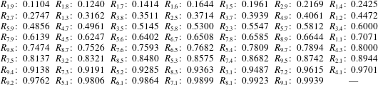
). Table 1 lists the frequencies
 $\unicode[STIX]{x1D714}$
(rounded off to four significant figures) associated with the low-order retracing rays
 $R_{i.j}$
with
 $i,j\leqslant 9$
. Note that
 $R_{\unicode[STIX]{x1D6FE}i.\unicode[STIX]{x1D6FE}j}$
for any
 $\unicode[STIX]{x1D6FE}$
are equivalent, and so only the cases with
 $\unicode[STIX]{x1D6FE}=1$
are listed. In the frequency range considered in the experiments of Boisson et al. (Reference Boisson, Lamriben, Maas, Cortet and Moisy2012),
 $\unicode[STIX]{x1D714}\in [0.60,0.73]$
, there are exactly three low-order retracing rays cases,
 $R_{i.j}$
with
 $i,j\leqslant 5$
. These are
 $R_{1.1}$
at
 $\unicode[STIX]{x1D714}=0.7071$
,
 $R_{3.4}$
at
 $\unicode[STIX]{x1D714}=0.600$
, and
 $R_{4.5}$
at
 $\unicode[STIX]{x1D714}=0.6247$
. For
 $\mathit{E}\approx 10^{-4.6}$
used in the experiments, and the energy norm in the plane that was used, there were no responses at or near these frequencies. However, it should be noted that the beams are viscously attenuated (Cortet, Lamriben & Moisy Reference Cortet, Lamriben and Moisy2010). They are strongest near the edges from where they are emitted, and lose intensity along their path. They also lose intensity upon wall reflections through the viscous boundary layers. So, for relatively large
 $\mathit{E}$
, there is little difference in the response from a low-order retracing case compared to a high-order case, or to a non-retracing case for that matter. This accounts for the observed near-constant response away from the single response peak at
 $\unicode[STIX]{x1D714}\approx 0.676$
. In order to detect a signature from a retracing ray case, it is desirable to use smaller
 $\mathit{E}$
. Even then, it is also important to use an appropriate measure. While the kinetic energy can provide a good measure for a smooth global quantity, such as an eigenmode, it does not do as well in quantifying the strength of a shear layer; the helicity variance
 $\unicode[STIX]{x1D6F4}_{H}^{2}$
turns out to be a better measure. This is consistent with the property that inertial waves are intrinsically helical (Davidson Reference Davidson2013, § 3.3.1).
Retracing rays,
 $R_{i.j}$
, with
 $i,j\leqslant 9$
, and their corresponding frequency (equivalent cases
 $R_{\unicode[STIX]{x1D6FE}i.\unicode[STIX]{x1D6FE}j}$
with
 $\unicode[STIX]{x1D6FE}\neq 1$
are not included).

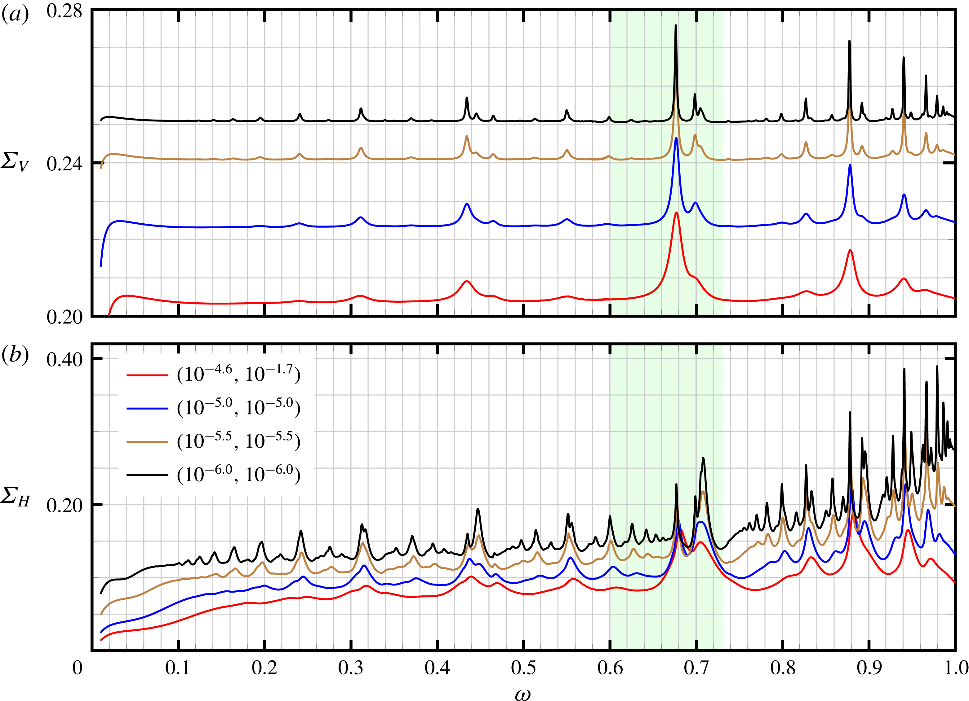
Variation of
 $(a)$
 $\unicode[STIX]{x1D6F4}_{V}$
and
 $(b)$
 $\unicode[STIX]{x1D6F4}_{H}$
with
 $\unicode[STIX]{x1D714}$
for
 $(\mathit{E},\unicode[STIX]{x1D716})$
as indicated. The shaded band corresponds to the
 $\unicode[STIX]{x1D714}$
range considered in Boisson et al. (Reference Boisson, Lamriben, Maas, Cortet and Moisy2012).

In order to further explore the system’s response to librational forcing, and clarify the interpretation of the response in terms of linear inviscid concepts, it is desirable to reduce both
 $\mathit{E}$
and
 $\unicode[STIX]{x1D716}$
. This is challenging both experimentally and numerically. Numerically, we have computed the responses not only for the
 $\mathit{E}$
,
 $\unicode[STIX]{x1D716}$
and
 $\unicode[STIX]{x1D714}$
values covered in the experimental study (Boisson et al.
Reference Boisson, Lamriben, Maas, Cortet and Moisy2012), but have also extended the ranges to
 $\mathit{E}\in [10^{-6},10^{-4.6}]$
, and
 $\unicode[STIX]{x1D716}$
as small as
 $10^{-6}$
. These much smaller
 $\mathit{E}$
and
 $\unicode[STIX]{x1D716}$
cases bring us a little closer to the linear inviscid limit. Also, we extended the frequency range to
 $\unicode[STIX]{x1D714}\in (0,1)$
with a very fine resolution
 $\unicode[STIX]{x1D6FF}\unicode[STIX]{x1D714}=0.001$
(with refinement about some major peaks using
 $\unicode[STIX]{x1D6FF}\unicode[STIX]{x1D714}=0.0005$
). Reducing
 $\mathit{E}$
progressively reveals more peaks in the responses, and the peaks that were present at the larger
 $\mathit{E}$
become sharper and shift slightly as the effects of viscous detuning are reduced.
Figure 3(a) is the
 $\unicode[STIX]{x1D6F4}_{V}$
–
 $\unicode[STIX]{x1D714}$
response diagram. Focusing on the response curve for
 $(\mathit{E},\unicode[STIX]{x1D716})=(2.65\times 10^{-5},0.02)\approx (10^{-4.6},10^{-1.7})$
, corresponding to the experiments of Boisson et al. (Reference Boisson, Lamriben, Maas, Cortet and Moisy2012), we find excellent qualitative agreement between their time-averaged kinetic energy response and our
 $\unicode[STIX]{x1D6F4}_{V}$
response. The quantitative differences are due to our use of a global measure (as noted earlier,
 $0.5\unicode[STIX]{x1D716}^{2}\unicode[STIX]{x1D6F4}_{V}^{2}$
is the time average of the kinetic energy in the cube volume, excluding boundary layer contributions) rather that the experimental use of only the two velocity components in the measurement plane (excluding 8 % of the plane in from the wall). The corresponding
 $\unicode[STIX]{x1D6F4}_{H}$
response at
 $(\mathit{E},\unicode[STIX]{x1D716})\approx (10^{-4.6},10^{-1.7})$
in figure 3(b) shows a clearer, but still broad, peak in the neighbourhood of
 $\unicode[STIX]{x1D714}=0.69$
corresponding to the slight bump in the energy response noted in the experiments and also present in our
 $\unicode[STIX]{x1D6F4}_{V}$
response. As discussed in Boisson et al. (Reference Boisson, Lamriben, Maas, Cortet and Moisy2012), this may be due to another eigenmode being resonantly excited, but being of higher order than
 $M_{2.1}$
it is more viscously damped at this
 $\mathit{E}$
, and also the bump is near
 $\unicode[STIX]{x1D714}=0.7071$
which corresponds to the lowest-order retracing ray
 $R_{1.1}$
. Given that the bump in
 $\unicode[STIX]{x1D6F4}_{V}$
becomes a clear peak in
 $\unicode[STIX]{x1D6F4}_{H}$
lends further weight to the interpretation of
 $R_{1.1}$
contributing to the response. Reducing
 $\mathit{E}$
sharpens the responses and helps to distinguish the contributions.
For
 $(\mathit{E},\unicode[STIX]{x1D716})=(10^{-6},10^{-6})$
, the highest peak in the
 $\unicode[STIX]{x1D6F4}_{V}$
response occurs at
 $\unicode[STIX]{x1D714}=0.676$
, which is close to the frequency of the eigenmode
 $M_{2.1}$
. There are two other peaks at
 $\unicode[STIX]{x1D714}=0.698$
and
 $0.705$
, and in the vicinity of these two peaks are the frequencies of the eigenmodes
 $M_{4.3}$
(
 $[4,5,+]$
in the notation of Boisson et al.
Reference Boisson, Lamriben, Maas, Cortet and Moisy2012) and
 $M_{6.6}$
(
 $[6,11,+]$
), which are both
 ${\mathcal{K}}_{z}\times {\mathcal{R}}_{\unicode[STIX]{x03C0}/2}$
invariant. There is also a small bump close to
 $\unicode[STIX]{x1D714}=0.62$
, but in the vicinity of this bump there are no low-order
 ${\mathcal{K}}_{z}\times {\mathcal{R}}_{\unicode[STIX]{x03C0}/2}$
symmetric eigenmodes. Also, in the vicinity of
 $\unicode[STIX]{x1D714}=0.7$
, the edge beams are being driven at approximately
 $45^{\circ }$
with respect to the rotation vector. Therefore, it is difficult to say if the peak in
 $\unicode[STIX]{x1D6F4}_{V}$
at
 $\unicode[STIX]{x1D714}=0.705$
is due to a resonance with the eigenmode
 $M_{6.6}$
or if it is due to the retracing ray
 $R_{1.1}$
. Actually, the response peak has contributions from both
 $M_{6.6}$
and
 $R_{1.1}$
. In the
 $\unicode[STIX]{x1D6F4}_{H}$
response, the highest peak occurs at
 $\unicode[STIX]{x1D714}=0.707$
, and this is very close to the
 $R_{1.1}$
frequency
 $\unicode[STIX]{x1D714}=1/\sqrt{2}\approx 0.7071$
.
Close-ups of the
 $\unicode[STIX]{x1D6F4}_{H}$
–
 $\unicode[STIX]{x1D714}$
response for
 $(\mathit{E},\unicode[STIX]{x1D716})=(10^{-6},10^{-6})$
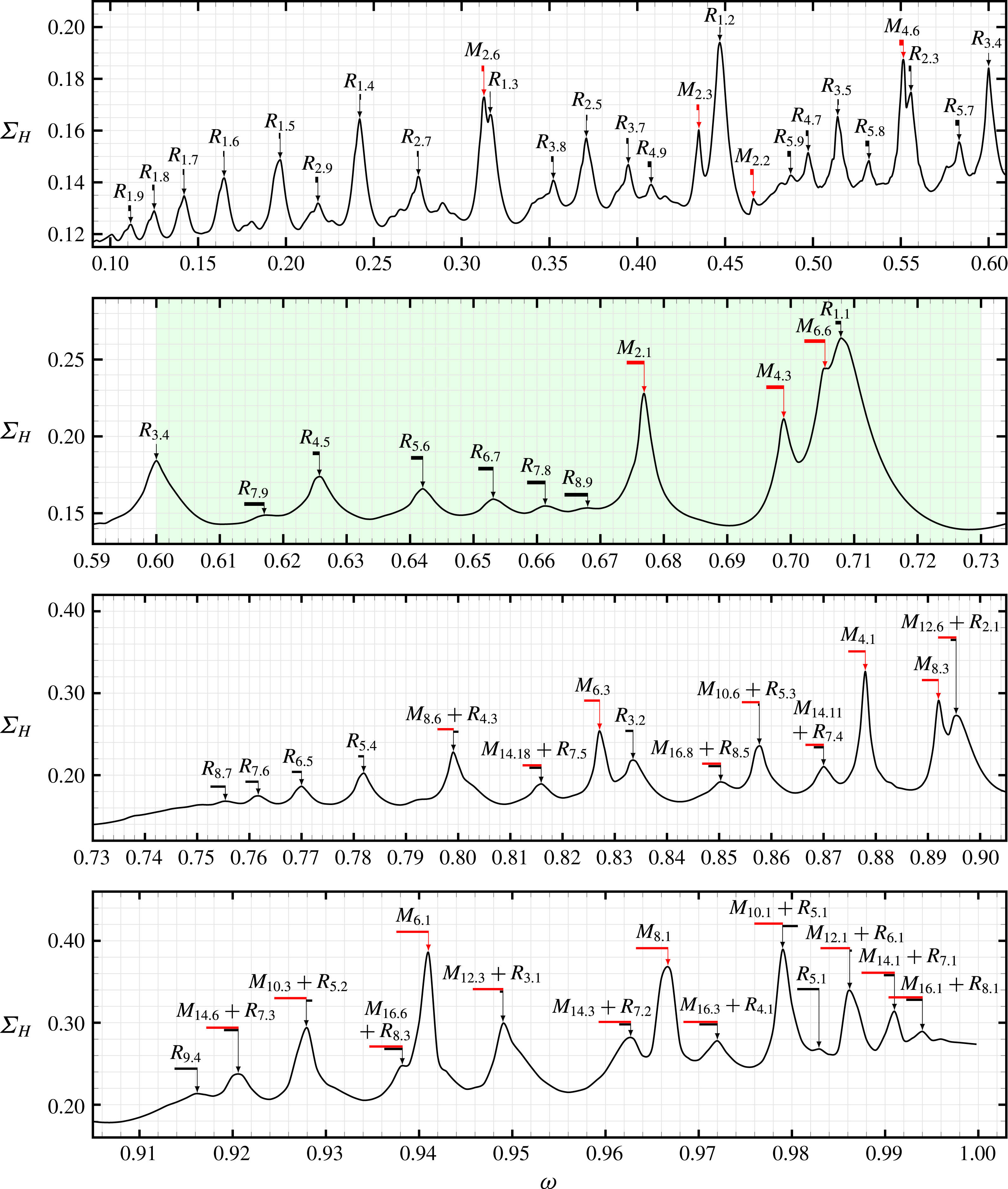
shown in figure 3, with the major peaks identified, along with the deviation from their nominal frequency (detuning). The detuning is indicated with a horizontal bar (black for
 $R_{i.j}$
and red for
 $M_{n.m}$
) whose ends are at the corresponding inviscid frequency and the peak’s frequency.

We now restrict our attention to the
 $\unicode[STIX]{x1D6F4}_{H}$
response diagram at
 $(\mathit{E},\unicode[STIX]{x1D716})=(10^{-6},10^{-6})$
, since
 $\unicode[STIX]{x1D6F4}_{H}$
is much better at capturing localized responses, such as beams, in the flow dynamics, while also detecting resonant low-order eigenmodes. In figure 3
 $(b)$
four dominant peaks are observed in the (highlighted) range
 $\unicode[STIX]{x1D714}\in [0.6,0.73]$
considered by Boisson et al. (Reference Boisson, Lamriben, Maas, Cortet and Moisy2012), at frequencies
 $\unicode[STIX]{x1D714}=0.677$
, 0.699, 0.705 and 0.708. In order to more clearly see the details, figure 4 is a close-up over the frequency range
 $\unicode[STIX]{x1D714}\in (0,1)$
, broken up into four subfigures. It includes identifications of the major peaks with either low-order retracing rays or low-order eigenmodes, and the associated viscous detuning (i.e. the difference between the peak frequency and the frequency of the associated retracing ray or eigenmode). The horizontal bars have one end with a vertical line drawn to the response peak and the other end of the bar is at the corresponding inviscid frequency; the width of the bar is the viscous detuning. In the following, we elaborate on how these identifications are arrived at.
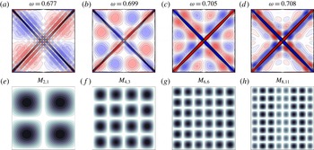
Contours of (a–d)
 $\unicode[STIX]{x1D714}_{x}$
in the vertical plane
 $x=0$
at the phase
 $\unicode[STIX]{x1D711}=\unicode[STIX]{x03C0}/2$
, for
 $(\mathit{E},\unicode[STIX]{x1D716})=(10^{-6},10^{-6})$
and
 $\unicode[STIX]{x1D714}$
as indicated, and (e–h) the normalized amplitude of
 $\unicode[STIX]{x1D714}_{x}$
of the inviscid inertial eigenmodes
 $M_{n.m}$
, with
 $n$
and
 $m$
as indicated, in the vertical plane
 $x=0$
. All contour levels are equispaced with
 $\unicode[STIX]{x1D714}_{x}\in [-2.5,2.5]$
for (a–d).

Figure 5 shows snapshots of
 $\unicode[STIX]{x1D714}_{x}$
in the vertical plane
 $x=0$
at phase
 $\unicode[STIX]{x1D711}=\unicode[STIX]{x03C0}/2$
for the frequencies
 $\unicode[STIX]{x1D714}$
of the four main peaks in figure 4, together with the normalized amplitude of
 $\unicode[STIX]{x1D714}_{x}$
of the matching low-order inviscid inertial eigenmodes
 $M_{n.m}$
, whose eigenfrequencies are close to these
 $\unicode[STIX]{x1D714}$
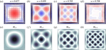
values. Figure 6 shows snapshots of
 $\unicode[STIX]{x1D714}_{z}$
at the same phase in the horizontal plane
 $z=0.45$
(close to the top wall), together with corresponding
 $\unicode[STIX]{x1D714}_{z}$
-amplitude of the eigenmodes in a horizontal plane. The online movies 2, 3, 4 and 5 are animations of these (both nonlinear simulations and corresponding inviscid inertial eigenmodes) over one libration period, providing additional insight.
Contours of (a–d)
 $\unicode[STIX]{x1D714}_{z}$
in the horizontal plane
 $z=0.45$
at the phase
 $\unicode[STIX]{x1D711}=\unicode[STIX]{x03C0}/2$
, for
 $(\mathit{E},\unicode[STIX]{x1D716})=(10^{-6},10^{-6})$
and
 $\unicode[STIX]{x1D714}$
as indicated, and (e–h) the normalized amplitude of the
 $\unicode[STIX]{x1D714}_{z}$
of the inviscid inertial eigenmodes
 $M_{n.m}$
, with
 $n$
and
 $m$
as indicated, in a horizontal plane. All contour levels equispaced with
 $\unicode[STIX]{x1D714}\in [-2.5,2.5]$
for (a–d). The second row (e–h) is the first row of the sequence of modes shown in figure 14.

At
 $\unicode[STIX]{x1D714}=0.677$
, the characteristic four cells in the vertical plane (figure 5
e) and one cell filling the horizontal plane (figure 6
e) of eigenmode
 $M_{2.1}$
, whose eigenfrequency is
 $\unicode[STIX]{x1D70E}\approx 0.6742$
, are easily recognizable in figures 5(a) and 6(a), respectively, and animated over one period in movie 2. The numerical simulations of
 $\unicode[STIX]{x1D714}_{x}$
in the vertical plane
 $x=0$
clearly show that the beams originating at the top and bottom edges are not retracing. The beams intersect the
 $z=0.45$
horizontal plane close to the vertical walls and produce minimal interference with the dominant eigenmode away from the edges. At
 $\unicode[STIX]{x1D714}=0.699$
the beams are more focused and more intense, and appear to be retracing (see figure 5
b), however the frequency is relatively far from
 $1/\sqrt{2}$
of the retracing ray
 $R_{1.1}$
. The nonlinear simulations (figures 5
b and 6
b) show the presence of eigenmode
 $M_{4.3}$
(whose eigenfrequency is
 $0.6962$
), featuring a distinct
 $4\times 4$
cell structure in the vertical plane
 $x=0$
and an easily identifiable pattern in the
 $z=0.45$
horizontal cut, which is only mildly affected by the beams; these are more clearly evident in the animation in movie 3. With the forcing frequency
 $\unicode[STIX]{x1D714}=0.705$
being closer to the retracing ray
 $R_{1.1}$
frequency, the flow is more dominated by the beams and the signature of a dominant eigenmode is harder to identify. The pattern of cells in the vertical plane
 $x=0$
in figure 5(c) can only be loosely related to the similar cut for eigenmode
 $M_{6.6}$
in figure 5(g) due to the increased interaction between the beams and the smaller sized cells of the eigenmode. Nevertheless, the horizontal cuts in figures 6(c,g) provide evidence of the presence of
 $M_{6.6}$
at that frequency, albeit at a weaker level compared to mode
 $M_{4.3}$
at frequency
 $\unicode[STIX]{x1D714}=0.699$
. Also note the aggregation, entrainment and reinforcement of the cell structures in the direction of the beams in figure 5(c); this is more apparent in the online movie 4 showing this simulation over one libration period. At
 $\unicode[STIX]{x1D714}=0.708$
, traces of eigenmodes have almost disappeared from the nonlinear simulations in figures 5(d) and 6(d), and the flow is completely dominated by the edge beams, with a resonance peak associated with the retracing ray
 $R_{1.1}$
being predominant in the
 $\unicode[STIX]{x1D6F4}_{H}$
response shown in figures 3 and 4. For comparison, we have included in figures 5(h) and 6(h) the next highest mode
 $M_{8.11}$
from the sequence in figures 14 and 17 (in appendix A), whose eigenfrequency closely matches the forcing frequency, and which might be expected to become more evident at yet smaller values of
 $\mathit{E}$
. This extrapolation is also supported by the observation that at forcing frequencies
 $\unicode[STIX]{x1D714}=0.677$
,
 $0.699$
and
 $0.705$
there is evidence in the nonlinear simulations of the near-resonant excitation of the dominant modes
 $M_{2.1}$
,
 $M_{4.3}$
and
 $M_{6.6}$
, with eigenfrequencies
 $0.6742$
,
 $0.6962$
and
 $0.7022$
; these all have approximately constant detuning (the difference between forcing frequency and eigenfrequency) of approximately
 $+0.003$
. The movie 5 is also suggestive of the presence of
 $M_{8.11}$
in the response, but it is highly deformed by the beams.
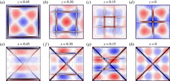
Contours of
 $(a-d)$
 $\unicode[STIX]{x1D714}_{z}$
at horizontal planes and
 $(e-h)$
 $\unicode[STIX]{x1D714}_{x}$
at vertical planes as indicated, at
 $(\mathit{E},\unicode[STIX]{x1D716})=(10^{-6},10^{-6})$
,
 $\unicode[STIX]{x1D714}=0.699$
and phase
 $\unicode[STIX]{x1D711}=\unicode[STIX]{x03C0}/2$
. All contour levels are equispaced with
 $\unicode[STIX]{x1D714}\in [-2.5,2.5]$
. See the online movies 6 and 7 for animations over one libration period.

At the vertical level
 $z=0.45$
, the eigenmode
 $M_{4.3}$
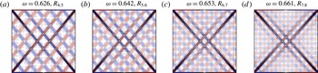
in figure 5(b) is only weakly perturbed by the beams emanating from the top edges. In order to better understand the interaction between the mode and the beams we consider the response at
 $\unicode[STIX]{x1D714}=0.699$
, examining
 $\unicode[STIX]{x1D714}_{z}$
at different horizontal planes
 $z=0$
,
 $0.15$
,
 $0.30$
and
 $0.45$
and
 $\unicode[STIX]{x1D714}_{x}$
at different vertical planes
 $x=0.45$
,
 $0.30$
,
 $0.15$
and
 $0$
. These are plotted in figure 7, showing the snapshots at the phase
 $\unicode[STIX]{x1D711}=\unicode[STIX]{x03C0}/2$
. Except for minor deformations due to beam interactions, the structure of the flow in these
 $z$
-planes retains the overall shape of the eigenmode
 $M_{4.3}$
(figure 6
f). The relative strength of the response in the different
 $z$
-planes is consistent with the dependence of
 $\unicode[STIX]{x1D714}_{z}$
on
 $z$
predicted by (A 23). With
 $n=4$
, the factor
 $\cos n\unicode[STIX]{x03C0}z$
in (A 23) is approximately
 $(1.00,-0.31,-0.81,0.81)$
at
 $z=(0.00,0.15,0.30,0.45)$
, and explains the relative signs and magnitudes at the various
 $z$
-levels. In particular, at
 $z=0.15$
the contribution from the mode is much weaker and hence more susceptible to be deformed or even overpowered by the beams (see figure 7
 $c$
). The plots in vertical
 $x$
-planes also show the
 $n=4$
vertical structure of
 $M_{4.3}$
, along with distortions resulting from the nonlinear interactions between the mode and the beams. The beams from the corners
 $(y,z)=(\pm 0.5,\pm 0.5)$
are clearly evident as they traverse each
 $x$
-plane at approximately
 $45^{\circ }$
. The beams from the corners
 $(x,z)=(\pm 0.5,\pm 0.5)$
appear horizontally at
 $z\approx x$
in each
 $x$
-plane.
While the snapshots in figure 7 help identify the presence of the mode
 $M_{4.3}$
at the different
 $z$
-levels and
 $x$
-levels, they do not provide a dynamic account of the impact of the beams on the mode. In movie 6, the animation of mode
 $M_{4.3}$
in a horizontal plane shows a clockwise progressive wave of cells in the plane, whereas the numerical simulations in the various
 $z$
-planes show that the beams tend to hinder this progression, pinning and distorting the cells in their vicinity, and confining other cells to a restricted space. For example, the four (blue) cells in figure 7(c) are confined to their respective quadrant, while the central cell is pinned at the centre, with a somewhat distorted structure. On the other hand, the central cell in figure 7(a) is unperturbed and free to rotate, while the four (red) outer cells are pinned by the beams. This differential interaction in different
 $z$
-planes, which is due to the vertical inclination of the beams, leads to a torsional forcing in the axial (vertical) direction. The dynamic interaction between the beams and mode in the
 $x$
-planes is depicted in movie 7.
Contours of
 $\unicode[STIX]{x1D714}_{x}$
in the vertical plane
 $x=0$
for
 $(\mathit{E},\unicode[STIX]{x1D716})=(10^{-6},10^{-6})$
and phase
 $\unicode[STIX]{x1D711}=\unicode[STIX]{x03C0}/2$
at
 $\unicode[STIX]{x1D714}$
as indicated. All contour levels equispaced with
 $\unicode[STIX]{x1D714}_{x}\in [-2.5,2.5]$
.

The range
 $\unicode[STIX]{x1D714}\in [0.6,0.73]$
also includes a cascade of peaks at the frequencies very close to those of the retracing rays
 $R_{3.4}$
,
 $R_{4.5}$
,
 $R_{5.6}$
,
 $R_{6.7}$
and
 $R_{7.8}$
illustrated in figure 8. These are indicated in the
 $\unicode[STIX]{x1D6F4}_{H}$
–
 $\unicode[STIX]{x1D714}$
response diagram in figure 4. At these frequencies, the flow is more dominated by the edge beams; their retracing contributes to increased phase coherence in the beams. The intensity of these beams and the height of the peaks decrease as the order of the beam (the number of reflections on horizontal and vertical walls) increases; the more reflections on the walls the greater the viscous attenuation of the beams in the boundary layers, and the farther they have to travel before reaching an edge, being viscously attenuated along the way.
We now consider the system’s response over the broader frequency range. In the range
 $\unicode[STIX]{x1D714}\in (0,0.6)$
, there is one notable peak at
 $\unicode[STIX]{x1D714}=0.434$
in the
 $\unicode[STIX]{x1D6F4}_{V}$
response for
 $(\mathit{E},\unicode[STIX]{x1D716})=(10^{-4.6},10^{-1.7})$
shown in figure 3
 $(a)$
. This peak corresponds to the inviscid inertial mode
 $M_{2.3}$
, with eigenfrequency
 $\unicode[STIX]{x1D70E}\approx 0.4339$
, and whose horizontal structure will be shown in figure 13 and its vertical structure in figure 16 (these figures are in the appendix A). This frequency is also close to the frequency
 $\unicode[STIX]{x1D714}\approx 0.4472$
of the retracing ray
 $R_{1.2}$
. There is a smaller bump in the
 $\unicode[STIX]{x1D6F4}_{V}$
response associated with
 $(\mathit{E},\unicode[STIX]{x1D716})=(10^{-4.6},10^{-1.7})$
at
 $\unicode[STIX]{x1D714}=0.312$
corresponding to
 $M_{2.6}$
, whose frequency
 $0.3115$
is also close to the frequency
 $\unicode[STIX]{x1D714}\approx 0.3162$
of retracing ray
 $R_{1.3}$
. The proximity of these resonant inviscid inertial modes and low-order retracing rays at the relatively large
 $\mathit{E}=10^{-4.6}$
results in a broad blended peak. Decreasing
 $\mathit{E}$
to
 $10^{-6}$
separates the contributions of modes and the beams into distinct peaks as the reduced viscous damping both sharpens the peaks and reduces their detuning.
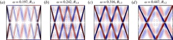
A sequence of peaks corresponding to retracing rays
 $R_{1.j}$
,
 $j=9\rightarrow 1$
with increasing
 $\unicode[STIX]{x1D714}$
cumulating at
 $\unicode[STIX]{x1D714}=1/\sqrt{2}$
for
 $R_{1,1}$
is also observed. The intensity of these beams increases with decreasing order
 $j$
(the number of reflections on the horizontal walls). Figure 9 illustrates some of these states.
Contours of
 $\unicode[STIX]{x1D714}_{x}$
in the vertical plane
 $x=0$
for
 $(\mathit{E},\unicode[STIX]{x1D716})=(10^{-6},10^{-6})$
at phase
 $\unicode[STIX]{x1D711}=\unicode[STIX]{x03C0}/2$
and
 $\unicode[STIX]{x1D714}$
as indicated. All contour levels equispaced with
 $\unicode[STIX]{x1D714}_{x}\in [-2.5,2.5]$
.

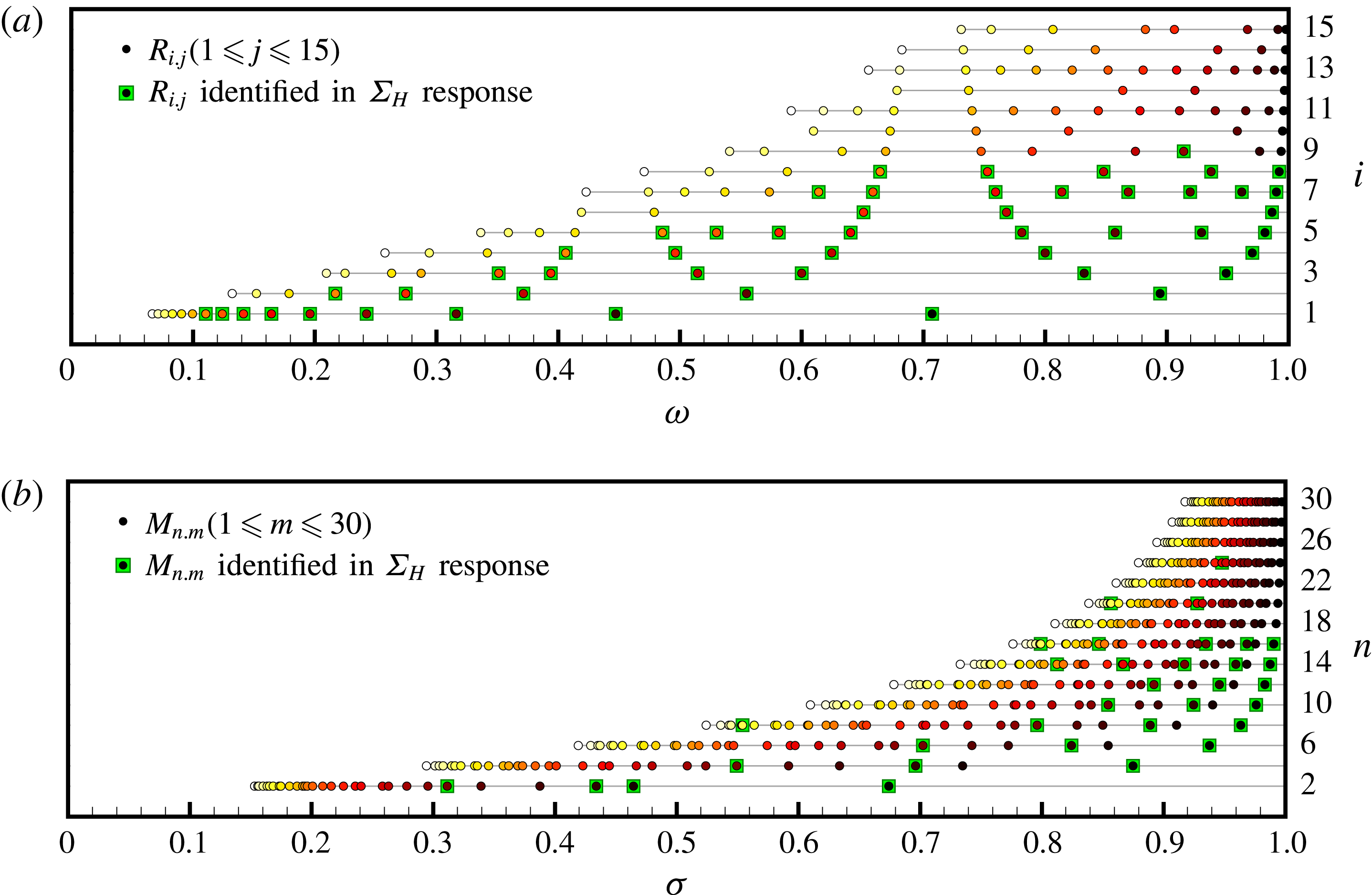
(a) Eigenfrequencies
 $\unicode[STIX]{x1D70E}$
of the inviscid inertial modes
 $M_{n.m}$
for
 $1\leqslant n$
,
 $m\leqslant 30$
(
 $n$
even), and (b) frequencies
 $\unicode[STIX]{x1D714}$
of the retracing rays
 $R_{i.j}$
for
 $1\leqslant i$
,
 $j\leqslant 15$
. Circles are coloured according to the value of
 $m$
, from dark red/black for low
 $m$
to light yellow/white for large
 $m$
in the range considered.

Contours of
 $(a-d)$
 $\unicode[STIX]{x1D714}_{x}$
in the vertical plane
 $x=0$
and
 $(e-h)$
 $\unicode[STIX]{x1D714}_{z}$
in the horizontal plane
 $z=0$
, for
 $(\mathit{E},\unicode[STIX]{x1D716})=(10^{-6},10^{-6})$
at phase
 $\unicode[STIX]{x1D711}=\unicode[STIX]{x03C0}/2$
and
 $\unicode[STIX]{x1D714}$
as indicated. All contour levels equispaced with
 $\unicode[STIX]{x1D714}_{x}\in [-2.5,2.5]$
.

We now turn our attention to the frequency range
 $\unicode[STIX]{x1D714}\in (0.73,1)$
. For the experimental conditions,
 $(\mathit{E},\unicode[STIX]{x1D716})=(10^{-4.6},10^{-1.7})$
, the
 $\unicode[STIX]{x1D6F4}_{V}$
response (figure 3
a) has relatively strong peaks associated with inertial modes
 $M_{4.1}$
and
 $M_{6.1}$
, and a weaker peak corresponding to
 $M_{8.1}$
. These peaks become more intense and localized for
 $(\mathit{E},\unicode[STIX]{x1D716})=(10^{-6},10^{-6})$
. A few other minor peaks emerge for
 $\unicode[STIX]{x1D714}\gtrsim 0.8$
, including one near
 $\unicode[STIX]{x1D714}=0.965$
corresponding to
 $M_{10.1}$
, but the overall response is at or marginally above the background response level. On the other hand, the
 $\unicode[STIX]{x1D6F4}_{H}$
response in figure 3(b) (also see the close-up in 4) reveals an abundance of peaks with increasing power as
 $\unicode[STIX]{x1D714}\rightarrow 1$
. The higher peak count in this range of
 $\unicode[STIX]{x1D714}$
corresponds to the higher number of both low-order inertial eigenmodes and retracing rays with frequency close to
 $1$
, illustrated in figure 10. This figure also illustrates the absence of either low-order retracing rays or inertial eigenmodes
 $M_{n.m}$
with
 $m=1,3,6$
in the vicinity of the
 $R_{1.1}$
frequency
 $\unicode[STIX]{x1D714}=1/\sqrt{2}$
. The
 $\unicode[STIX]{x1D6F4}_{H}$
response also picks up the sequence of retracing beams
 $R_{j+1.j}$
,
 $j=7\rightarrow 1$
. The response at
 $\unicode[STIX]{x1D714}=0.799$
shows significant contributions from both
 $R_{4.3}$
and
 $M_{8.6}$
, and at
 $\unicode[STIX]{x1D714}=0.896$
the response peak has contributions from both
 $R_{2.1}$
and
 $M_{4.3}$
. In fact, all major peaks for
 $\unicode[STIX]{x1D714}\gtrsim 0.8$
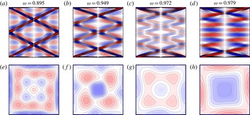
consist of contributions from both retracing rays and inertial modes, as illustrated in figure 11. For example, figure 11(a) clearly shows the presence of
 $R_{2.1}$
in the
 $\unicode[STIX]{x1D714}_{x}$
contours in the plane
 $x=0$
at
 $\unicode[STIX]{x1D714}=0.895$
, with
 $M_{12.6}$
(more generally of an eigenmode
 $M_{12.m}$
) recognizable in the background, while figure 11(e) shows the
 $\unicode[STIX]{x1D714}_{z}$
structure in the horizontal plane
 $z=0$
of
 $M_{12.6}$
(more generally of an eigenmode
 $M_{n.6}$
). In figure 11
 $(b)$
, the vertical structure of
 $\unicode[STIX]{x1D714}_{z}$
at
 $\unicode[STIX]{x1D714}=0.949$
indicates the strong presence of
 $R_{3.1}$
, while the number of changes of background colour close to the median (vertical line
 $y\approx 0$
) together with the plot of
 $\unicode[STIX]{x1D714}_{z}$
in a horizontal plane in figure 11(f) show the presence of eigenmode
 $M_{12.3}$
. As the forcing frequency
 $\unicode[STIX]{x1D714}$
approaches 1, the beams (retracing or not) become increasingly more horizontal and are subject to increasing dissipative interactions with the top and bottom wall boundary layers and many reflections at the sidewalls. As a result, it is more difficult for these beams to retain coherence all the way to the mid-vertical section of the cube, thereby leaving a fairly undisturbed picture of the inertial modes away from the top and bottom endwalls. Figures 11(c,g) at
 $\unicode[STIX]{x1D714}=0.972$
, close to the frequencies of
 $R_{4.1}$
and
 $M_{16.3}$
, and figure 11(d,h) at
 $\unicode[STIX]{x1D714}=0.979$
, close to the frequencies of
 $R_{5.1}$
and
 $M_{10.1}$
, illustrate these effects. The beam
 $R_{5.1}$
can be better observed with minimal interference from
 $M_{10.1}$
at
 $\unicode[STIX]{x1D714}=0.983$
. The combination
 $M_{10.1}+R_{5.1}$
is also the first of a sequence of modes and beams
 $M_{2i.1}+R_{i.1}$
,
 $i=5,6,7,8$
, observed in unison in the
 $\unicode[STIX]{x1D6F4}_{H}$
and the vorticity responses in the range
 $0.975\lesssim \unicode[STIX]{x1D714}<1$
.
Whether an inviscid eigenmode or inertial edge beam, or a combination, is observed in the response at a particular forcing frequency
 $\unicode[STIX]{x1D714}$
depends on the separation between the corresponding natural frequencies of these eigenmodes and beams (these are listed in tables 1 and 2 and illustrated in figure 10 for the low-order modes and retracing beams), compared to detuning due to viscous and nonlinear effects. For relatively large
 $\mathit{E}=10^{-4.6}$
viscous effects spread the influence of the modes and beams over a wide
 $\unicode[STIX]{x1D714}$
-bandwidth, with contributions from both combining to a single peak. This is especially so in the
 $\unicode[STIX]{x1D6F4}_{V}$
response. For example, see the response at
 $\unicode[STIX]{x1D714}=0.879$
, where
 $M_{4.1}$
and
 $R_{2.1}$
compete, and
 $\unicode[STIX]{x1D714}=0.941$
, where
 $M_{6.1}$
and
 $R_{3.1}$
compete. At smaller Ekman number
 $\mathit{E}=10^{-6}$
the peaks become sharper, making the distinction between the two contributions possible, especially in the
 $\unicode[STIX]{x1D6F4}_{H}$
response. However, contributions from higher-order modes and beams become apparent and the same difficulties repeat on a smaller frequency range, much like what happens when focusing in on a fractal. Still, at
 $\mathit{E}=10^{-6}$
many modes and beams appear combined into single peaks because of the proximity of their natural frequencies. These typically manifest themselves during different phases of the librational period or in different cross-sections of the cube. For example, at
 $\mathit{E}=10^{-6}$
,
 $M_{2i.1}$
appears in the same response with
 $R_{i.1}$
, for
 $i=5,6,7$
and 8;
 $M_{2i.3}$
with
 $R_{i.2}$
for
 $i=2,5,7$
and 8 (note that
 $R_{8.2}=R_{4.1}$
);
 $M_{2i.6}$
with
 $R_{i.3}$
for
 $i=4,5,7$
and 8; and
 $M_{2i.18}$
with
 $R_{i.5}$
for
 $i=7$
and 8. At certain frequencies multiple eigenmodes were also observed at different phases together with a retracing beam. For example,
 $M_{4i.11}$
and
 $M_{2i.3}$
with
 $R_{i.2}$
at
 $\unicode[STIX]{x1D714}=0.928$
for
 $i=5$
and at
 $\unicode[STIX]{x1D714}=0.949$
for
 $i=6$
, and
 $M_{4i.25}$
and
 $M_{2i.6}$
with
 $R_{i.3}$
at
 $\unicode[STIX]{x1D714}=0.799$
for
 $i=4$
and at
 $\unicode[STIX]{x1D714}=0.858$
for
 $i=6$
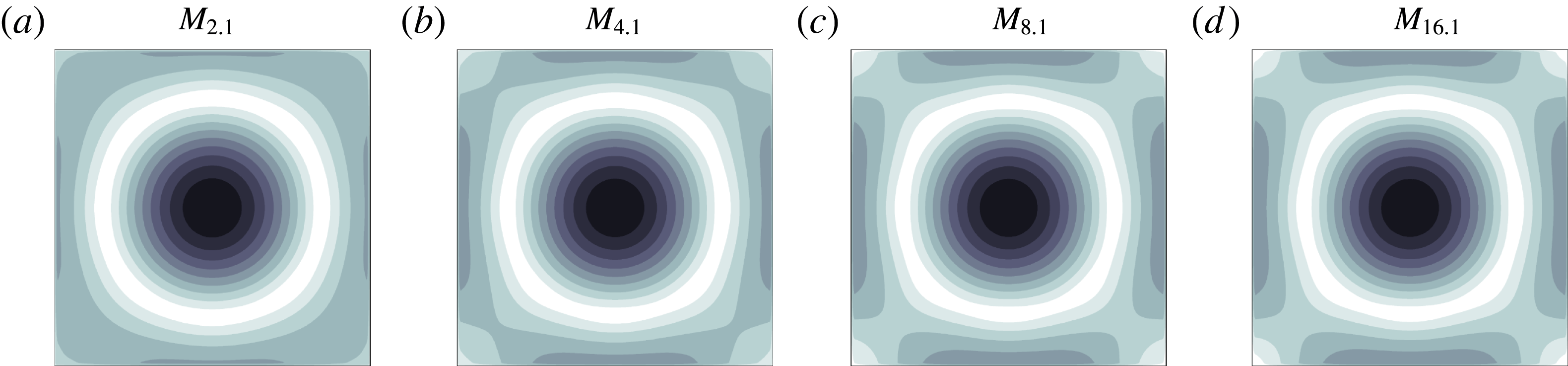
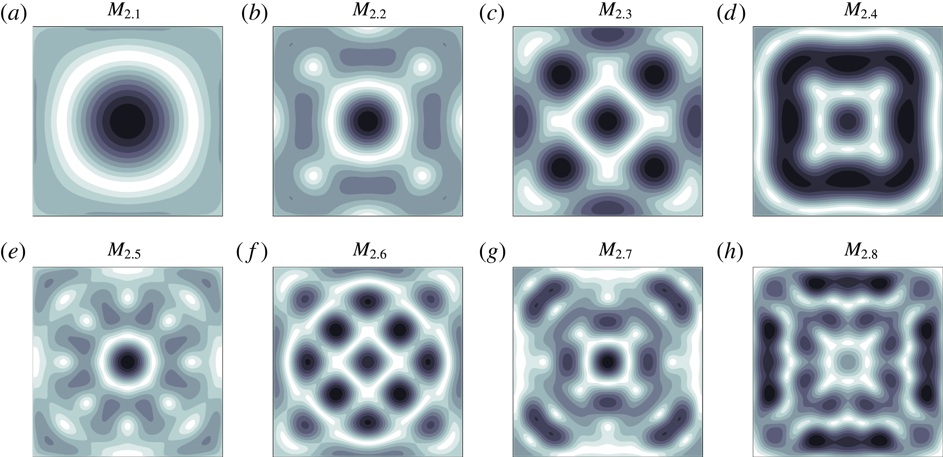
. The higher-order eigenmodes (omitted from figure 4) can be thought of as spatial (pseudo-)harmonics of the lower-order modes, with slightly different temporal eigenfrequencies, as will be exemplified by figures 14
 $(c,f)$
and 17
 $(c,f)$
.
 ${\mathcal{K}}_{z}\times {\mathcal{R}}_{\unicode[STIX]{x03C0}/2}$
-symmetric inviscid inertial modes,
 $M_{n.m}$
, with even
 $n\leqslant 12$
,
 $m\leqslant 10$
, together with their corresponding frequency.

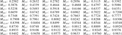
The multiplicity of observed natural eigenmodes at specific forcing frequencies, their association with retracing beams, and the accumulation of natural eigenfrequencies at certain frequencies all raise the issue of degeneracy. The numerical multiplicity of certain eigenfrequencies, illustrated for example by modes
 $M_{6.2}$
and
 $M_{10.6}$
with frequencies identical up to four significant decimal digits listed in table 2, tends to support the idea. On the other hand, the progressive narrowing of the response peaks as
 $\mathit{E}$
gets smaller might suggest otherwise. A full analysis of this complex issue is beyond the scope of the present study.
Movie 8 summarizes the response
 $\unicode[STIX]{x1D714}_{x}$
in the plane
 $x=0$
at phase
 $\unicode[STIX]{x1D711}=\unicode[STIX]{x03C0}/2$
as
 $\unicode[STIX]{x1D714}$
increases from
 $0.001$
to
 $0.999$
with steps of
 $0.001$
. It clearly illustrates the vertical structure of the beams, which are stronger when they are retracing, and at certain peak frequencies the low-order eigenmodes are very predominant. As
 $\unicode[STIX]{x1D714}$
passes through these peaks the change in dominance between beams and modes creates a flashing effect in the movie.
5 Discussion and conclusions
The flow response of a rapidly rotating fluid-filled cube to low-amplitude librational forcing was investigated numerically over the entire range of forcing frequencies supporting inertial waves responses. The enclosed geometry has natural inviscid inertial eigenmodes which the librational forcing can excite resonantly, and in the physical situation governed by the Navier–Stokes equations the resonant response is subject to viscous damping and detuning, and nonlinear saturation. The geometry of the cube and the nature of the librational forcing imparts the system with invariance to
 ${\mathcal{K}}_{z}\times {\mathcal{R}}_{\unicode[STIX]{x03C0}/2}$
consisting of reflection about the horizontal midplane and rotation of
 $\unicode[STIX]{x03C0}/2$
about the rotation axis of the cube. The eigenmodes, coming from the Euler equations linearized about the state of solid-body rotation, are invariant to additional symmetries that the Navier–Stokes equations solutions are not, as a consequence of the nonlinear terms and the Euler force describing the libration in the cube frame of reference. For sufficiently low libration amplitudes the Navier–Stokes response flow is invariant to
 ${\mathcal{K}}_{z}\times {\mathcal{R}}_{\unicode[STIX]{x03C0}/2}$
and only the eigenmodes that are
 ${\mathcal{K}}_{z}\times {\mathcal{R}}_{\unicode[STIX]{x03C0}/2}$
invariant are resonantly excited. The Navier–Stokes response also consists of internal shear layers, called edge beams as they emerge from edges where the horizontal walls of the cube meet the vertical walls. These are driven by the periodic fluxes in the horizontal wall boundary layers. In the interior they follow the directions of the characteristics of the linear inviscid problem, and reflect off walls preserving these directions. They are thinner and more intense with decreasing Ekman number, and the degree to which the velocity and vorticity vectors align (enhanced helicity) along these beams also increases with decreasing Ekman number. For finite Ekman numbers, they are viscously attenuated along their paths and upon wall reflections, and they interact nonlinearly when they cross or are in close proximity. For some libration frequencies, they return to an edge after completing a small number of reflections off the walls. These low-order retracing cases tend to have increased phase coherence.
The eigenmodes and the beams correspond to two different mechanisms: the modes are intrinsic to the geometry of the rotating container, while the beams are extrinsically driven by the details of the body forcing (e.g., libration). In trying to determine what the response to external forcing is due to, the measure used to quantify the response can emphasize different aspects of the response. First and foremost, any measure needs to be of the flow response away from the boundary layers, as most measures are completely swamped by the boundary layer contributions. Many studies (e.g., Boisson et al. Reference Boisson, Lamriben, Maas, Cortet and Moisy2012; Sauret et al. Reference Sauret, Cébron, Le Bars and Le Dizés2012) use a kinetic energy norm as the measure. The problem is that at the moderate Ekman numbers usually used, the contribution from the beams, regardless of whether they are retracing or not, tend to give a dominant near-constant response throughout the whole frequency range, and only the eigenmodes with the very lowest orders contribute an additional amount allowing their detection. Other experiments use a probe measuring pressure drop across the container (e.g., Aldridge & Toomre Reference Aldridge and Toomre1969), and this measure is also able to detect resonant responses from low-order modes, but not any signal from the internal beams. Other numerical investigations have used a vorticity norm which has been able to detect peak responses from both resonant eigenmodes and retracing beams (e.g., Lopez & Marques Reference Lopez and Marques2014; Gutierrez-Castillo & Lopez Reference Gutierrez-Castillo and Lopez2017). Here, we have found that a measure based on the variance in the helicity results in a clear detection of both resonant low-order eigenmodes and retracing beams, and as the Ekman number is reduced, the associated response peaks sharpen and shift in accord with the reduced viscous damping and detuning. The measure utilizes the intrinsic helical nature of the inertial responses.
It is of interest to compare the responses in the librating cube to those in a librating cylinder. The librating cylinder also has responses that consist of eigenmode resonances or phase coherence in retracing beams (Gutierrez-Castillo & Lopez Reference Gutierrez-Castillo and Lopez2017). In the cylinder, the Kelvin modes also come with a variety of symmetries, but the symmetry of the librating cylinder Navier–Stokes problem has
 ${\mathcal{K}}_{z}\times SO(2)$
symmetry. The
 ${\mathcal{K}}_{z}$
symmetry is the reflection about the horizontal midplane, as in the librating cube, and
 $SO(2)$
is the invariance to all rotations about the rotation axis. This continuous symmetry is replaced by invariance to a single member,
 ${\mathcal{R}}_{\unicode[STIX]{x03C0}/2}$
, the invariance to a rotation of
 $\unicode[STIX]{x03C0}/2$
about the rotation axis for the cube. As in the cube, low-amplitude librational forcing of the cylinder results in flow responses that have the symmetries of the system, and so only the axisymmetric reflection symmetric Kelvin modes are excited in the librating cylinder, just as only the
 ${\mathcal{K}}_{z}\times {\mathcal{R}}_{\unicode[STIX]{x03C0}/2}$
symmetric eigenmodes are excited in the librating cube. The beams in the librating cylinder are also much simpler. They form axisymmetric cones emanating from the edges where the cylinder endwalls meet the sidewall, whereas in the librating cube, as the beams emerge from straight edges, they form plane shear layers in the interior that intersect orthogonally. Of course, in the cylinder the conical beams also intersect orthogonally. Another difference is that in the librating cylinder, the flow is driven via viscous torque, whereas in the librating cube, since the motion of the vertical walls is not purely in their tangential direction, there is a significant contribution from the pressure torque driving the flow. How this difference manifests in the limit
 $\mathit{E}\rightarrow 0$
between the two geometries would be interesting to explore. This issue has been previously considered for librating spheroids (Wu & Roberts Reference Wu and Roberts2013). In a very recent study of libration-driven flows in ellipsoidal shells, in which the flow is strongly influenced by the pressure torque associated with the solid boundary motions having a normal component to their motion, Lemasquerier et al. (Reference Lemasquerier, Grannan, Vidal, Cébron, Favier, Le Bars and Aurnou2017) conclude: ‘Thus, the relative importance between localized shear layers and global inertial modes remains to be clarified, especially when both the forcing and the Ekman number are decreased.’ The present results provide a systematic study addressing precisely this issue. Although we have used
 $\mathit{E}=10^{-6}\ll 1$
,
 $\unicode[STIX]{x1D716}=10^{-6}\ll 1$
, and
 $\unicode[STIX]{x1D716}\mathit{E}^{-1/2}=10^{-3}\ll 1$
, the response to librational forcing still has significant viscous damping and detuning (
 $\mathit{E}$
is still too large for these effects to be negligible) and nonlinear saturation of resonances as well as nonlinear interactions within retracing beams lead to enhanced phase coherence, and in particular, nonlinear interactions between the resonantly excited eigenmodes and the beams (regardless of whether they retrace or not) lead to localized pinning and deformations (
 $\unicode[STIX]{x1D716}\mathit{E}^{-1/2}$
is still too large for nonlinear interactions to be negligible). It is unclear if there is a regime with
 $\mathit{E}\neq 0$
and
 $\unicode[STIX]{x1D716}\neq 0$
yet both small enough to have negligible viscous and nonlinear effects. On the other hand, it also still remains to be determined for small
 $\mathit{E}$
how large
 $\unicode[STIX]{x1D716}$
needs to be for the synchronous
 ${\mathcal{K}}\times {\mathcal{R}}_{\unicode[STIX]{x03C0}/2}$
forced response to lose stability.
Acknowledgements
This work was partially supported by National Science Foundation grant CBET-1336410. The computations were performed on the Saguaro Cluster of ASU Research Computing and School of Mathematical and Statistical Sciences computing facilities. The authors thank Jason Yalim for his expertise and valuable help in setting up some of these computations.
Supplementary movies
Supplementary movies are available at https://doi.org/10.1017/jfm.2018.157.
Appendix A. Computation of
 $\boldsymbol{{\mathcal{K}}}_{\boldsymbol{z}}\times \boldsymbol{{\mathcal{R}}}_{\unicode[STIX]{x03C0}\boldsymbol{/2}}$
-symmetric inviscid inertial modes

In order to keep the notation compact, in appendix A we shall denote
 ${\mathcal{R}}_{\unicode[STIX]{x03C0}/2}$
as
 ${\mathcal{R}}$
and use
 $\dot{\;\,}$
for
 $\unicode[STIX]{x2202}/\unicode[STIX]{x2202}t$
. The
 ${\mathcal{K}}_{z}$
-symmetric inviscid inertial modes are solutions of (2.4) of the form
 $$\begin{eqnarray}M_{n}(x,y,z,t):=\left[\begin{array}{@{}c@{}}u_{n}(x,y,t)\\ v_{n}(x,y,t)\\ 0\\ p_{n}(x,y,t)\end{array}\right]\cos (n\unicode[STIX]{x03C0}z)+\left[\begin{array}{@{}c@{}}0\\ 0\\ w_{n}(x,y,t)\\ 0\end{array}\right]\sin (n\unicode[STIX]{x03C0}z),\end{eqnarray}$$
with
 $n$
even to enforce boundary conditions at
 $z=\pm 0.5$
. Substitution into (2.4) yields
 $$\begin{eqnarray}\left[\begin{array}{@{}c@{}}\dot{u}_{n}\\ \dot{v}_{n}\end{array}\right]+2\left[\begin{array}{@{}r@{}}-v_{n}\\ u_{n}\end{array}\right]=-\unicode[STIX]{x1D735}p_{n},\quad {\dot{w}}_{n}=n\unicode[STIX]{x03C0}p_{n},\quad \unicode[STIX]{x1D735}\boldsymbol{\cdot }\left[\begin{array}{@{}c@{}}u_{n}\\ v_{n}\end{array}\right]+n\unicode[STIX]{x03C0}w_{n}=0,\end{eqnarray}$$
for each value of
 $n$
. Elimination of
 $p_{n}$
and
 $w_{n}$
leads to
 $$\begin{eqnarray}\dot{\boldsymbol{u}}_{n}+2{\mathcal{R}}\boldsymbol{u}_{n}=\frac{1}{(n\unicode[STIX]{x03C0})^{2}}\unicode[STIX]{x1D735}(\unicode[STIX]{x1D735}\boldsymbol{\cdot }\dot{\boldsymbol{u}}_{n}),\quad \boldsymbol{u}_{n}\boldsymbol{\cdot }\boldsymbol{n}|_{\unicode[STIX]{x2202}{\mathcal{S}}}=0,\quad \boldsymbol{u}_{n}=\left[\begin{array}{@{}c@{}}u_{n}\\ v_{n}\end{array}\right],\end{eqnarray}$$
where here
 $\boldsymbol{n}$
denotes the normal at the edges of the horizontal square cross-section
 ${\mathcal{S}}$
.
 ${\mathcal{R}}_{\unicode[STIX]{x03C0}/2}$
-symmetric solutions of (A 3), and thus of (2.4), are obtained as superpositions
 $$\begin{eqnarray}\boldsymbol{u}_{n}(x,y,t)=\mathop{\sum }_{k}p_{k,n}(t)\boldsymbol{v}_{k}(x,y)+\mathop{\sum }_{\ell }q_{\ell ,n}(t){\mathcal{R}}\boldsymbol{v}_{\ell ^{\prime }}(x,y),\end{eqnarray}$$
of
 ${\mathcal{R}}_{\unicode[STIX]{x03C0}/2}$
-symmetric basis functions
 $$\begin{eqnarray}\boldsymbol{v}_{k}(x,y):=\left[\begin{array}{@{}r@{}}\sin (k_{1}\unicode[STIX]{x03C0}x)\cos (k_{2}\unicode[STIX]{x03C0}y)\\ \cos (k_{2}\unicode[STIX]{x03C0}x)\sin (k_{1}\unicode[STIX]{x03C0}y)\end{array}\right],\quad {\mathcal{R}}\boldsymbol{v}_{\ell ^{\prime }}(x,y):=\left[\begin{array}{@{}r@{}}-\text{cos}(\ell _{1}\unicode[STIX]{x03C0}x)\sin (\ell _{2}\unicode[STIX]{x03C0}y)\\ \sin (\ell _{2}\unicode[STIX]{x03C0}x)\cos (\ell _{1}\unicode[STIX]{x03C0}y)\end{array}\right],\end{eqnarray}$$
where
 $k=(k_{1},k_{2})$
,
 $\ell =(\ell _{1},\ell _{2})$
, and
 $\ell ^{\prime }=(\ell _{2},\ell _{1})$
are integer pairs. The restrictions
 $k_{1}\neq 0$
even and
 $\ell _{1}$
odd guarantee that
 $\boldsymbol{u}_{n}$
satisfies the boundary condition in (A 3). The orthogonality property
 $$\begin{eqnarray}(\boldsymbol{v}_{k},{\mathcal{R}}\boldsymbol{v}_{\ell ^{\prime }}):=2\int _{-0.5}^{0.5}\int _{-0.5}^{0.5}\boldsymbol{v}_{k}(x,y)\boldsymbol{\cdot }{\mathcal{R}}\boldsymbol{v}_{\ell ^{\prime }}(x,y)\;\text{d}x\,\text{d}y=0,\end{eqnarray}$$
for any
 $k$
and
 $\ell$
, is a direct consequence of the symmetry about
 $x=y$
of the domain of integration. The functions
 $$\begin{eqnarray}\left.\begin{array}{@{}c@{}}\unicode[STIX]{x1D719}_{k}=\unicode[STIX]{x1D735}\boldsymbol{\cdot }\boldsymbol{v}_{k}=k_{1}\unicode[STIX]{x03C0}(\cos (k_{1}\unicode[STIX]{x03C0}x)\cos (k_{2}\unicode[STIX]{x03C0}y)+\cos (k_{2}\unicode[STIX]{x03C0}x)\cos (k_{1}\unicode[STIX]{x03C0}y)),\\ \unicode[STIX]{x1D713}_{\ell }=\unicode[STIX]{x1D735}\boldsymbol{\cdot }{\mathcal{R}}\boldsymbol{v}_{\ell ^{\prime }}=\ell _{1}\unicode[STIX]{x03C0}(\sin (\ell _{1}\unicode[STIX]{x03C0}x)\sin (\ell _{2}\unicode[STIX]{x03C0}y)-\sin (\ell _{2}\unicode[STIX]{x03C0}x)\sin (\ell _{1}\unicode[STIX]{x03C0}y)),\end{array}\right\}\end{eqnarray}$$
correspond to symmetrized versions of the potential and stream functions appearing in Maas (Reference Maas2003, p. 386), with gradients
 $$\begin{eqnarray}\unicode[STIX]{x1D735}\unicode[STIX]{x1D719}_{k}=\unicode[STIX]{x03C0}^{2}(-k_{1}^{2}\boldsymbol{v}_{k}-k_{1}k_{2}\boldsymbol{v}_{k^{\prime }}),\quad \unicode[STIX]{x1D735}\unicode[STIX]{x1D713}_{\ell }=\unicode[STIX]{x03C0}^{2}(-\ell _{1}^{2}{\mathcal{R}}\boldsymbol{v}_{\ell ^{\prime }}+\ell _{1}\ell _{2}{\mathcal{R}}\boldsymbol{v}_{\ell }).\end{eqnarray}$$
Substitution of (A 4) into (A 3), and using (A 7) and (A 8), yields
 $$\begin{eqnarray}\displaystyle & & \displaystyle \mathop{\sum }_{k}{\dot{p}}_{k,n}\boldsymbol{v}_{k}+\mathop{\sum }_{\ell }\dot{q}_{\ell ,n}{\mathcal{R}}\boldsymbol{v}_{\ell ^{\prime }}+2\mathop{\sum }_{k}p_{k,n}{\mathcal{R}}\boldsymbol{v}_{k}-2\mathop{\sum }_{\ell }q_{\ell ,n}\boldsymbol{v}_{\ell ^{\prime }}\nonumber\\ \displaystyle & & \displaystyle \quad =\frac{1}{(n\unicode[STIX]{x03C0})^{2}}\left(\mathop{\sum }_{k}{\dot{p}}_{k,n}\unicode[STIX]{x1D735}\unicode[STIX]{x1D719}_{k}+\mathop{\sum }_{\ell }\dot{q}_{\ell ,n}\unicode[STIX]{x1D735}\unicode[STIX]{x1D713}_{\ell }\right)\nonumber\\ \displaystyle & & \displaystyle \quad =-\mathop{\sum }_{k}{\dot{p}}_{k,n}\frac{k_{1}^{2}}{n^{2}}\boldsymbol{v}_{k}-\mathop{\sum }_{k}{\dot{p}}_{k,n}\frac{k_{1}k_{2}}{n^{2}}\boldsymbol{v}_{k^{\prime }}-\mathop{\sum }_{\ell }\dot{q}_{\ell ,n}\frac{\ell _{1}^{2}}{n^{2}}{\mathcal{R}}\boldsymbol{v}_{\ell ^{\prime }}+\mathop{\sum }_{\ell }\dot{q}_{\ell ,n}\frac{\ell _{1}\ell _{2}}{n^{2}}{\mathcal{R}}\boldsymbol{v}_{\ell }.\qquad \quad\end{eqnarray}$$
Multiplying by
 $\boldsymbol{v}_{i}$
and
 ${\mathcal{R}}\boldsymbol{v}_{j^{\prime }}$
, respectively, integrating and using (A 6), implies
 $$\begin{eqnarray}\displaystyle & & \displaystyle \mathop{\sum }_{k}{\dot{p}}_{k,n}(\boldsymbol{v}_{i},\boldsymbol{v}_{k})-2\mathop{\sum }_{\ell }q_{\ell ,n}(\boldsymbol{v}_{i},\boldsymbol{v}_{\ell ^{\prime }})\nonumber\\ \displaystyle & & \displaystyle \quad =-\mathop{\sum }_{k}{\dot{p}}_{k,n}\frac{k_{1}^{2}}{n^{2}}(\boldsymbol{v}_{i},\boldsymbol{v}_{k})-\mathop{\sum }_{k}{\dot{p}}_{k,n}\frac{k_{1}k_{2}}{n^{2}}(\boldsymbol{v}_{i},\boldsymbol{v}_{k^{\prime }}),\end{eqnarray}$$
 $$\begin{eqnarray}\displaystyle & & \displaystyle \mathop{\sum }_{\ell }\dot{q}_{\ell ,n}(\boldsymbol{v}_{j^{\prime }},\boldsymbol{v}_{\ell ^{\prime }})+2\mathop{\sum }_{k}p_{k,n}(\boldsymbol{v}_{j^{\prime }},\boldsymbol{v}_{k})\nonumber\\ \displaystyle & & \displaystyle \quad =-\mathop{\sum }_{\ell }\dot{q}_{\ell ,n}\frac{\ell _{1}^{2}}{n^{2}}(\boldsymbol{v}_{j^{\prime }},\boldsymbol{v}_{\ell ^{\prime }})+\mathop{\sum }_{\ell }\dot{q}_{\ell ,n}\frac{\ell _{1}\ell _{2}}{n^{2}}(\boldsymbol{v}_{j^{\prime }},\boldsymbol{v}_{\ell }),\end{eqnarray}$$
i.e.
 $$\begin{eqnarray}\displaystyle \unicode[STIX]{x1D63C}_{n}[{\dot{p}}_{k,n}]=2\unicode[STIX]{x1D63D}_{n}[q_{\ell ,n}],\quad \unicode[STIX]{x1D63E}_{n}[\dot{q}_{\ell ,n}]=-2\unicode[STIX]{x1D63F}_{n}[p_{k,n}], & & \displaystyle\end{eqnarray}$$
with
 $$\begin{eqnarray}\left.\begin{array}{@{}l@{}}\unicode[STIX]{x1D63C}_{n}=[(\unicode[STIX]{x1D63C}_{n})_{i,k}]=\left[\left(1+{\displaystyle \frac{k_{1}^{2}}{n^{2}}}\right)(\boldsymbol{v}_{i},\boldsymbol{v}_{k})+{\displaystyle \frac{k_{1}k_{2}}{n^{2}}}(\boldsymbol{v}_{i},\boldsymbol{v}_{k^{\prime }})\right],\unicode[STIX]{x1D63D}_{n}=[(\unicode[STIX]{x1D63D}_{n})_{i,\ell }]=\left[(\boldsymbol{v}_{i},\boldsymbol{v}_{\ell ^{\prime }})\right],\\ \unicode[STIX]{x1D63E}_{n}=[(\unicode[STIX]{x1D63E}_{n})_{j,\ell }]=\left[\left(1+{\displaystyle \frac{\ell _{1}^{2}}{n^{2}}}\right)(\boldsymbol{v}_{j^{\prime }},\boldsymbol{v}_{\ell ^{\prime }})-{\displaystyle \frac{\ell _{1}\ell _{2}}{n^{2}}}(\boldsymbol{v}_{j^{\prime }},\boldsymbol{v}_{\ell })\right],\unicode[STIX]{x1D63F}_{n}=[(\unicode[STIX]{x1D63F}_{n})_{j,k}]=\left[(\boldsymbol{v}_{j^{\prime }},\boldsymbol{v}_{k})\right].\end{array}\right\}\end{eqnarray}$$
The coefficients of these (infinite) matrices can be evaluated from
 $$\begin{eqnarray}(\boldsymbol{v}_{i},\boldsymbol{v}_{k})=\left(\text{sinc}\frac{k_{1}-i_{1}}{2}-\text{sinc}\frac{k_{1}+i_{1}}{2}\right)\left(\text{sinc}\frac{k_{2}-i_{2}}{2}+\text{sinc}\frac{k_{2}+i_{2}}{2}\right),\end{eqnarray}$$
where
 $\text{sinc}(x)=\sin (\unicode[STIX]{x03C0}x)/(\unicode[STIX]{x03C0}x)$
for
 $x\neq 0$
and
 $\text{sinc}(0)=1$
. The Ansätze
 $$\begin{eqnarray}[p_{k,n}]=\boldsymbol{p}_{n}\sin 2\unicode[STIX]{x1D70E}_{n}t,\quad [q_{\ell ,n}]=\boldsymbol{q}_{n}\cos 2\unicode[STIX]{x1D70E}_{n}t,\end{eqnarray}$$
yield the generalized eigenvalue problem
 $$\begin{eqnarray}\unicode[STIX]{x1D70E}_{n}\left[\begin{array}{@{}cc@{}}\unicode[STIX]{x1D63C}_{n} & 0\\ 0 & \unicode[STIX]{x1D63E}_{n}\end{array}\right]\left[\begin{array}{@{}c@{}}\boldsymbol{p}_{n}\\ \boldsymbol{ q}_{n}\end{array}\right]=\left[\begin{array}{@{}cc@{}}0 & \unicode[STIX]{x1D63D}_{n}\\ \unicode[STIX]{x1D63F}_{n} & 0\end{array}\right]\left[\begin{array}{@{}c@{}}\boldsymbol{p}_{n}\\ \boldsymbol{ q}_{n}\end{array}\right].\end{eqnarray}$$
In the Galerkin approach, the sets of index pairs
 $i$
and
 $j$
are the same as the sets of pairs
 $k$
and
 $\ell$
, respectively. For practical computation, these sets are truncated, for each
 $n$
, to
 $$\begin{eqnarray}\displaystyle 0\leqslant k_{1}+k_{2},\quad \ell _{1}+\ell _{2}\leqslant 2N, & & \displaystyle\end{eqnarray}$$
for some positive integer
 $N$
chosen to be independent of
 $n$
. With a consistent ordering of the pairs, the (finite) matrices
 $\unicode[STIX]{x1D63C}_{n}$
and
 $\unicode[STIX]{x1D63E}_{n}$
are symmetric positive definite, and
 $\unicode[STIX]{x1D63D}_{n}^{\text{T}}=\unicode[STIX]{x1D63F}_{n}$
. The restrictions
 $k_{2}$
even and
 $\ell _{2}$
odd further guarantee that the gradients (A 8) and all terms in (A 3) are
 ${\mathcal{R}}_{\unicode[STIX]{x03C0}/2}$
-symmetric. The matrices
 $\unicode[STIX]{x1D63C}_{n}$
and
 $\unicode[STIX]{x1D63E}_{n}$
then have dimension
 $M=N(N+1)/2$
. Upon reordering to keep
 $k$
and
 $k^{\prime }$
, and
 $\ell$
and
 $\ell ^{\prime }$
, consecutive, these matrices become block diagonal, with
 $1\times 1$
or
 $2\times 2$
blocks. Specifically,
 $$\begin{eqnarray}\left.\begin{array}{@{}l@{}}(\unicode[STIX]{x1D63C}_{n})_{\{k,k^{\prime }\},\{k,k^{\prime }\}}=I_{2}+\boldsymbol{k}\boldsymbol{k}^{\text{T}}\quad \text{with }\boldsymbol{k}:={\displaystyle \frac{1}{n}}\left[\begin{array}{@{}r@{}}k_{1}\\ k_{2}\end{array}\right]\text{ if }k_{2}\neq 0,k_{1},\\ (\unicode[STIX]{x1D63C}_{n})_{k,k}=c_{k}\left(1+\boldsymbol{k}^{\text{T}}\boldsymbol{k}\right)\quad \text{with }c_{k}:=\left\{\begin{array}{@{}ll@{}}2 & \text{if }k_{2}=0,\\ 1 & \text{if }k_{2}=k_{1},\end{array}\right.\\ (\unicode[STIX]{x1D63E}_{n})_{\{\ell ,\ell ^{\prime }\},\{\ell ,\ell ^{\prime }\}}=I_{2}+\boldsymbol{\ell }\boldsymbol{\ell }^{\text{T}}\quad \text{with }\boldsymbol{\ell }:={\displaystyle \frac{1}{n}}\left[\begin{array}{@{}r@{}}\ell _{1}\\ -\ell _{2}\end{array}\right]\text{ if }\ell _{2}\neq \ell _{1},\\ (\unicode[STIX]{x1D63E}_{n})_{\ell ,\ell }=1\quad \text{if }\ell _{2}=\ell _{1}.\end{array}\right\}\end{eqnarray}$$
On the other hand, the matrices
 $\unicode[STIX]{x1D63D}_{n}$
and
 $\unicode[STIX]{x1D63F}_{n}$
are full,
 $$\begin{eqnarray}(\unicode[STIX]{x1D63D}_{n})_{k,\ell }=(-1)^{[1+0.5(k_{1}+k_{2}+\ell _{1}+\ell _{2})]}\left(\frac{4}{\unicode[STIX]{x03C0}}\right)^{2}\frac{k_{1}\ell _{1}}{(k_{1}^{2}-\ell _{2}^{2})(k_{2}^{2}-\ell _{1}^{2})}=(\unicode[STIX]{x1D63F}_{n})_{\ell ,k}.\end{eqnarray}$$
The symmetric positive definite matrices
 $\unicode[STIX]{x1D63C}_{n}$
and
 $\unicode[STIX]{x1D63E}_{n}$
are trivially diagonalized, and their square roots
 $\unicode[STIX]{x1D63C}_{n}^{1/2}$
and
 $\unicode[STIX]{x1D63E}_{n}^{1/2}$
are easily computed. The truncated generalized eigenvalue problem (A 16) can then be recast as
 $$\begin{eqnarray}\unicode[STIX]{x1D70E}_{n}\left[\begin{array}{@{}c@{}}\unicode[STIX]{x1D63C}_{n}^{1/2}\boldsymbol{p}_{n}\\[5.0pt] \unicode[STIX]{x1D63E}_{n}^{1/2}\boldsymbol{q}_{n}\end{array}\right]=\left[\begin{array}{@{}cc@{}}0 & \boldsymbol{S}_{n}\\[5.0pt] \boldsymbol{S}_{n}^{\text{T}} & 0\end{array}\right]\left[\begin{array}{@{}c@{}}\unicode[STIX]{x1D63C}_{n}^{1/2}\boldsymbol{p}_{n}\\[5.0pt] \unicode[STIX]{x1D63E}_{n}^{1/2}\boldsymbol{q}_{n}\end{array}\right]\quad \text{with }\boldsymbol{S}_{n}=\unicode[STIX]{x1D63C}_{n}^{-1/2}\unicode[STIX]{x1D63D}_{n}\unicode[STIX]{x1D63E}_{n}^{-1/2},\end{eqnarray}$$
i.e.,
 $\unicode[STIX]{x1D63C}_{n}^{1/2}\boldsymbol{p}_{n}$
and
 $\unicode[STIX]{x1D63E}_{n}^{1/2}\boldsymbol{q}_{n}$
are the left and right singular vectors of
 $\boldsymbol{S}_{n}$
, respectively, associated with each singular value
 $\unicode[STIX]{x1D70E}_{n}$
. These singular values are naturally ordered by decreasing magnitude, and indexed by an integer
 $1\leqslant m\leqslant M$
. Table 2 lists the eigenfrequencies (rounded off to four significant figures) of the low-order modes
 $M_{n.m}$
with even
 $n\leqslant 12$
and
 $m\leqslant 10$
.
Each
 $m$
determines a pair
 $(\,\boldsymbol{p}_{n},\boldsymbol{q}_{n})$
, and a solution
 $\boldsymbol{u}_{n}$
of (A 3) using (A 4) and (A 5), with corresponding fields
 $(w_{n},p_{n})$
obtained from (A 2), and result in an eigenmode
 $M_{n}=M_{n.m}$
in (A 1) indexed by
 $n$
and
 $m$
. Note that the meaning of
 $m$
here differs from the one in the notation
 $[n,m,+]$
used in Boisson et al. (Reference Boisson, Lamriben, Maas, Cortet and Moisy2012), where both
 ${\mathcal{R}}_{\unicode[STIX]{x03C0}/2}$
-symmetric and
 $\overline{{\mathcal{R}}}_{\unicode[STIX]{x03C0}/2}$
-symmetric were computed, with interlacing frequencies
 $\unicode[STIX]{x1D70E}_{n}$
. Table 3 summarizes the connection between the two notations for lower values of
 $m$
.
Normalized amplitude
 $a_{n.1}(x,y)$
of
 $\unicode[STIX]{x1D714}_{z}$
of
 $M_{n.1}$
for
 $n$
as indicated.

Correspondence between inviscid inertial eigenmode notations (
 $N$
large).

Normalized amplitude
 $a_{2.m}(x,y)$
of
 $\unicode[STIX]{x1D714}_{z}$
of
 $M_{2.m}$
for
 $m$
as indicated.

Normalized amplitude
 $a_{n.m}(x,y)$
of
 $\unicode[STIX]{x1D714}_{z}$
of
 $M_{n.m}$
for
 $m$
as indicated, with frequencies accumulating at frequency
 $0.7071$
of the retracing ray
 $R_{1.1}$
.

Normalized amplitude
 $a_{n.1}(y,z)$
of
 $\unicode[STIX]{x1D714}_{x}$
of
 $M_{n.1}$
for
 $n$
as indicated.

Normalized amplitude
 $a_{2.m}(y,z)$
of
 $\unicode[STIX]{x1D714}_{x}$
of
 $M_{2.m}$
for
 $m$
as indicated.

Normalized amplitude
 $a_{[n,m]}(y,z)$
of
 $\unicode[STIX]{x1D714}_{x}$
of
 $M_{n.m}$
for
 $n$
and
 $m$
as indicated, with frequencies accumulating at the frequency
 $0.7071$
of the retracing ray
 $R_{1.1}$
.

Quantities of interest may be computed from (A 1). For example, the vertical component of vorticity,
 $\unicode[STIX]{x1D714}_{z}$
, of
 $M_{n.m}$
in the plane
 $z=0$
can be evaluated as
 $$\begin{eqnarray}\displaystyle \unicode[STIX]{x1D714}_{z}(x,y,0,t) & = & \displaystyle \left(\frac{\unicode[STIX]{x2202}v_{n}}{\unicode[STIX]{x2202}x}-\frac{\unicode[STIX]{x2202}u_{n}}{\unicode[STIX]{x2202}y}\right)(x,y,0,t)\nonumber\\ \displaystyle & = & \displaystyle \left(\mathop{\sum }_{k}\frac{k_{2}}{k_{1}}(\,\boldsymbol{p}_{n})_{k}\unicode[STIX]{x1D713}_{k}(x,y)\right)\sin 2\unicode[STIX]{x1D70E}_{n}t+\left(\mathop{\sum }_{\ell }\frac{\ell _{2}}{\ell _{1}}(\boldsymbol{q}_{n})_{\ell }\unicode[STIX]{x1D719}_{\ell }(x,y)\right)\cos 2\unicode[STIX]{x1D70E}_{n}t,\nonumber\\ \displaystyle & & \displaystyle\end{eqnarray}$$
with
 $\boldsymbol{p}_{n}$
and
 $\boldsymbol{q}_{n}$
obtained from the
 $m$
th singular vectors
 $\unicode[STIX]{x1D63C}_{n}^{1/2}\boldsymbol{p}_{n}$
and
 $\unicode[STIX]{x1D63E}_{n}^{1/2}\boldsymbol{q}_{n}$
in the singular value decomposition (SVD) of
 $\boldsymbol{S}_{n}$
. The expression (A 21) can be converted to polar form
 $$\begin{eqnarray}\unicode[STIX]{x1D714}_{z}(x,y,0,t)=a_{n}(x,y)\cos \left(2\unicode[STIX]{x1D70E}_{n}t-\unicode[STIX]{x1D703}_{n}(x,y)\right),\end{eqnarray}$$
in order to extract the amplitude,
 $a_{n}(x,y)$
, and phase,
 $\unicode[STIX]{x1D703}_{n}(x,y)$
. Since
 $$\begin{eqnarray}\unicode[STIX]{x1D714}_{z}(x,y,z,t)=\unicode[STIX]{x1D714}_{z}(x,y,0,t)\cos n\unicode[STIX]{x03C0}z,\end{eqnarray}$$
the trace of
 $\unicode[STIX]{x1D714}_{z}$
in any horizontal plane (constant
 $z$
) retains its shape as a function of
 $x$
and
 $y$
.
The parities of
 $k$
and
 $\ell$
imply
 $\unicode[STIX]{x1D713}_{k}=\unicode[STIX]{x1D719}_{\ell }=0$
, and therefore
 $a_{n}=0$
, on the boundaries, for any
 $n$
and mode
 $m$
. Certain modes exhibit large amplitude
 $a_{n}$
close to the boundary and numerical (Gibbs) oscillations may appear when evaluating
 $a_{n}$
on finer grids. These difficulties led Maas (Reference Maas2003) to abandon the spectral approach in favour of finite elements (Nurijanyan, Bokhove & Maas Reference Nurijanyan, Bokhove and Maas2013). Instead, we evaluate
 $a_{n}$
on a uniform
 $2N\times 2N$
grid, apply two passes of a local low-pass filter with 9-point stencil
 $$\begin{eqnarray}\frac{1}{(1+2|x|)(1+2|y|)}\left[\begin{array}{@{}ccc@{}}|xy| & |y| & |xy|\\ |x| & 1 & |x|\\ |xy| & |y| & |xy|\end{array}\right],\end{eqnarray}$$
(equivalent to a 25-point stencil in the domain interior), and use a local (spline) interpolation onto a grid mapped from a (possibly finer) uniform grid via the map
 $f(s)=\sin (\unicode[STIX]{x03C0}s)/2$
(with
 $s=x,\,y$
) in order to better capture sharp variations of
 $a_{n}$
along the edges. The filtering (A 24) is equivalent to standard linear smoothing close to the boundaries, but leaves the solution at the centre unchanged.
Similarly, the
 $x$
-component of the vorticity in the plane
 $x=0$
,
 $$\begin{eqnarray}\displaystyle \unicode[STIX]{x1D714}_{x}(0,y,z,t) & = & \displaystyle \left(\frac{\unicode[STIX]{x2202}w_{n}}{\unicode[STIX]{x2202}y}-\frac{\unicode[STIX]{x2202}v_{n}}{\unicode[STIX]{x2202}z}\right)(0,y,z,t)\nonumber\\ \displaystyle & = & \displaystyle \left[n\unicode[STIX]{x03C0}\sin n\unicode[STIX]{x03C0}z\mathop{\sum }_{k}(\,\boldsymbol{p}_{n})_{k}\left(\left[1+\frac{k_{1}^{2}}{n^{2}}\right]\sin k_{1}\unicode[STIX]{x03C0}y+\frac{k_{1}k_{2}}{n^{2}}\sin k_{2}\unicode[STIX]{x03C0}y\right)\right]\sin 2\unicode[STIX]{x1D70E}_{n}t,\nonumber\\ \displaystyle & & \displaystyle\end{eqnarray}$$
also vanishes on the domain boundary.
Increasing
 $N$
increases the size
 $M$
of
 $\boldsymbol{S}_{n}$
and the computational cost of the SVD. Note that to compute mode
 $m_{\max }$
, one only requires the determination of modes
 $1\leqslant m\leqslant m_{\max }$
, and a sparse version of the SVD (e.g. svds in Matlab) provides an efficient way to determine
 $\boldsymbol{p}_{n.m}$
and
 $\boldsymbol{q}_{n.m}$
. In fact, the bulk of the computational cost lies in the reconstruction of a mode itself on fine grids.
Convergence to
 $M_{n.m}$
as
 $N$
increases happens first for low
 $m$
values, associated with singular vectors with low spatial variation. In our computations of the eigenmodes, we used
 $N=100$
. The progression of
 $M_{n.m}$
as
 $n$
increases with fixed
 $m$
is illustrated in figure 12 for
 $m=1$
(also compare modes
 $M_{2.6}$
in figure 13 and
 $M_{6.6}$
in figure 14).
Figures 13 and 16 illustrate the first eight modes
 $M_{2.m}$
associated with
 $n=2$
. Figures 14 and 17 show a sequence of similar modes
 $M_{n.m}$
with increasing
 $n$
and
 $m=m(n)$
and frequency
 $\unicode[STIX]{x1D70E}_{n.m}$
converging to the frequency
 $1/\sqrt{2}$
of the retracing ray
 $R_{1.1}$
.
The approach described here differs from the Rao–Proudman approach used in Rao (Reference Rao1966) and Maas (Reference Maas2003) in several ways: (i) the expansion (A 4) automatically enforces the
 ${\mathcal{R}}_{\unicode[STIX]{x03C0}/2}$
-symmetry of the square horizontal cross-section on the velocity field, while Rao and Maas only enforced
 ${\mathcal{R}}_{\unicode[STIX]{x03C0}}$
-symmetry in general rectangular cross-sections; (ii) the components (A 5) in the decomposition (A 4) are neither irrotational nor divergence-free, yet still satisfy an orthogonality relation (A 6), in contrast with Rao and Maas’s approach based on the Helmholtz decomposition of
 $\boldsymbol{u}_{n}$
and subsequent projections onto subspaces of irrotational and divergence-free velocity fields; (iii) only positive frequencies
 $\unicode[STIX]{x1D70E}_{n}$
are computed, via an SVD problem, rather than both positive and negative frequencies obtained directly via a generalized eigenvalue problem similar to (A 16). Failure to explicitly enforce symmetry in (A 16), e.g., using (A 13) with (A 14), was also found to give incorrect results (complex modes) when
 $N\gtrsim 20$
.