1 Introduction
Shock tubes have proven themselves to be an important tool in understanding the complex phenomena of compressible fluid mechanics. Their original widespread popularity has largely been owed to their ability to consistently capture highly compressible physics at a reduced scale. Due to this, their use has also become a key part of the engineering design process in many fields, with perhaps the most notable field being aircraft design (Stever & Bisplinghoff Reference Stever and Bisplinghoff1954). In many problems, shock tubes have been adopted as a capable tool in the reproduction and better understanding of the underlying physics.
One application where shock tubes have gained considerable attention in recent years is volcanic eruptions. Shock tubes have been used to recreate features of volcanic eruptions at a more controlled, reduced scale. While not every aspect of the eruptions is able to be experimentally captured in a shock tube, experiments provide invaluable insight into the complex multiphase physics of these systems. In many cases, the eruption physics studied in shock tubes work under the assumption that the magma has already been fragmented. Fragmentation is the breakup of a continuous volume of molten rock into discrete pieces (Fowler et al. Reference Fowler, Scheu, Lee and McGuinness2010; Gonnermann Reference Gonnermann2015). The magma itself is composed of molten rock and compressed gases. At low depths and high pressures, the gases are mostly dissolved in the magma. As the magma rises, the gas will be exsolved due to a pressure-dependent solubility of its constituents. Gas bubbles will be created at nucleation sites and they will eventually grow and coalesce with each other. While there are multiple fragmentation mechanisms, in low-viscosity magma, the growth of bubbles causes rapid expansion that will rip the magma into fragments (Gonnermann Reference Gonnermann2015). These fragments will often solidify and potentially collide and be broken apart into smaller fragments. Due to their solidification, the magmatic fragments can be thought of as solid particles in a surrounding gas. As the fragments reach the volcanic vent interface, they may be discharged to the surrounding atmosphere in different ways which can be used to characterize the type of volcanic eruption. Thus, understanding the underlying multiphase physics of the rising mixture may help explain unexplored field observations. For this reason, shock tube experiments have been relied upon for valuable insight which is used in conjunction with historical measurements to better understand volcanic activity.
A shock tube experiment for volcanic eruptions was originally proposed and studied by Kieffer & Sturtevant (Reference Kieffer and Sturtevant1984). In their work, the focus was mainly on single-phase jet dynamics at the exit of a shock tube. To accomplish this, they performed experiments with four different shock tube gases, which were Freon 12, Freon 22, nitrogen and helium. Following this, Anilkumar (Reference Anilkumar1989) performed the first recorded experiments that we could find of a gas–solid multiphase shock tube in his dissertation which was published only a few years later (Anilkumar, Sparks & Sturtevant Reference Anilkumar, Sparks and Sturtevant1993). In this work, two types of particles were packed together to form a particle bed, which included manufactured glass beads and sieved volcanic ash collected from previous eruptions. These particle beds were rapidly depressurized in a shock tube apparatus. The experiments were more exploratory in nature and mainly focused on qualitative flow characteristics for different experimental inputs. These inputs included variation of particle sizes, particle bed arrangements and even flow visualization techniques. Despite the qualitative nature of the work, it has proved to be foundational, laying the groundwork for numerous future investigations.
In the following decade, various theoretical work was done to expand on the ideas originally proposed by Kieffer & Sturtevant (Reference Kieffer and Sturtevant1984). This includes Turcotte et al. (Reference Turcotte, Ockendon, Ockendon and Cowley1990) and Woods (Reference Woods1995) who presented similar models for the expansion of a multiphase mixture from a one-dimensional shock tube theory. Following this, Cagnoli et al. (Reference Cagnoli, Barmin, Melnik and Sparks2002) performed experiments similar to Anilkumar (Reference Anilkumar1989) and Anilkumar et al. (Reference Anilkumar, Sparks and Sturtevant1993) which quantified key characteristics of the depressurized gas–solid flows. In their experiments, both a wider range of shock tube pressures and smaller glass particles were investigated when compared to Anilkumar (Reference Anilkumar1989) and Anilkumar et al. (Reference Anilkumar, Sparks and Sturtevant1993). Additionally, Cagnoli et al. (Reference Cagnoli, Barmin, Melnik and Sparks2002) presented a theoretical model similar to Turcotte et al. (Reference Turcotte, Ockendon, Ockendon and Cowley1990) and Woods (Reference Woods1995) which was combined with standard shock tube theory to estimate the velocities and pressures in their cases. Following this, Chojnicki, Clarke & Phillips (Reference Chojnicki, Clarke and Phillips2006) performed similar experiments but at the extreme condition where the initial particle bed filled the entire high pressure section of the shock tube. They found that the particles decreased the generated shock strength and suggested that the multiphase shock tube model may need to be altered to include inter-phase momentum exchange between the particles and gas.
The physical process of fragmentation itself was experimentally investigated by Alatorre-Ibargüengoitia et al. (Reference Alatorre-Ibargüengoitia, Scheu, Dingwell, Delgado-Granados and Taddeucci2010) and McGuinness, Scheu & Fowler (Reference McGuinness, Scheu and Fowler2012) in similar multiphase shock tube experiments. Instead of glass particles, Alatorre-Ibargüengoitia et al. (Reference Alatorre-Ibargüengoitia, Scheu, Dingwell, Delgado-Granados and Taddeucci2010) used drilled samples of volcanic rocks that were pressurized with Argon gas and then externally heated. In this case, the molten rock would fragment resulting in a gas–particle mixture that rose up the shock tube. In their analysis, a theoretical model for the ejection of material, similar to the models of Turcotte et al. (Reference Turcotte, Ockendon, Ockendon and Cowley1990), Woods (Reference Woods1995) and Cagnoli et al. (Reference Cagnoli, Barmin, Melnik and Sparks2002), was presented, which also included modifications due to energy consumption by fragmentation of the samples. More recently, McGuinness & Singh (Reference McGuinness and Singh2015) developed a one-dimensional model explaining the formation of slab-like structures in the particle bed at early times in a multiphase shock tube. In their model, relevant conservation equations were solved to find when the gas-induced effective stress in the particle bed exceeds the bed cohesion, resulting in the bed rupturing. Their model was then found to be in good agreement when compared against the seminal experiments of Anilkumar (Reference Anilkumar1989) and Anilkumar et al. (Reference Anilkumar, Sparks and Sturtevant1993).
With the recent advances in computational methods and architectures, there is now a great opportunity to complement shock tube experiments with computer simulations and gain invaluable insight into such types of flows. In fact, a comprehensive review and comparison of numerous computational and numerical models for volcanic eruptions was given by Costa et al. (Reference Costa, Suzuki, Cerminara, Devenish, Ongaro, Herzog, Van Eaton, Denby, Bursik and de’ Michieli Vitturi2016). While such models can be directly applied to specific volcanic geometries, such as with Ongaro et al. (Reference Ongaro, Neri, Menconi, de’ Michieli Vitturi, Marianelli, Cavazzoni, Erbacci and Baxter2008), there have been fewer simulations of the aforementioned laboratory shock tube experiments. In 2007, detailed single-phase simulations of shock tubes similar to those originally proposed by Kieffer & Sturtevant (Reference Kieffer and Sturtevant1984) were performed by Haselbacher, Balachandar & Kieffer (Reference Haselbacher, Balachandar and Kieffer2007). Following this, an air–water shock tube problem was simulated by La Spina, de’ Michieli Vitturi & Clarke (Reference La Spina, de’ Michieli Vitturi and Clarke2017) for validation, prior to it being applied to model volcanic eruptions. In 2018, Marjanovic et al. (Reference Marjanovic, Hackl, Shringarpure, Annamalai, Jackson and Balachandar2018) simulated the propagation of rarefaction waves over arrays of stationary spheres at high-resolution. However, each of these simulations did not account for the movement and tracking of individual particles, which occurs in the multiphase shock tube experiments of Anilkumar (Reference Anilkumar1989), Anilkumar et al. (Reference Anilkumar, Sparks and Sturtevant1993), Cagnoli et al. (Reference Cagnoli, Barmin, Melnik and Sparks2002) and Chojnicki et al. (Reference Chojnicki, Clarke and Phillips2006). This is in part due to the challenge of modelling such flows. These particulate mixtures can be classified as a dispersed multiphase flow, meaning that particles are dispersed in a surrounding gas.
In dispersed multiphase flow modelling, the three most common modelling approaches are: (i) direct numerical simulation, (ii) the two-fluid (Euler–Euler) model and (iii) the point-particle (Euler–Lagrange) model (Balachandar & Eaton Reference Balachandar and Eaton2010). In direct numerical simulation, the finest scales of a flow must be resolved through a computational mesh where the governing equations are discretized. For a dispersed multiphase flow, this necessitates a mesh that is much smaller than the size of each individual particle. With current computational power this is clearly unrealistic for even moderate scale systems. The two-fluid approach is one alternative to direct numerical simulation where the grid may be much coarser. This allows simulation of much larger problem sizes than direct numerical simulation. However, this comes with the added penalty of volume filtering the discretized governing equations on the computational mesh since the finer scales are not resolvable. Filtering is performed for both the gas and the particle phases in the two-fluid approach, which means that the particles are treated as a continuum and individual interactions are not realizable. In contrast, the point-particle model only filters the gas phase and every particle is individually tracked. Due to this, along with recent computational and algorithmic advances, we have chosen the point-particle approach to model the multiphase shock tube simulations in this work (Zwick & Balachandar Reference Zwick and Balachandar2019). (Both two-fluid and point-particle approaches have been successfully used to model volcanic eruptions. Examples of this include Ongaro et al. (Reference Ongaro, Clarke, Voight, Neri and Widiwijayanti2012) and Cerminara, Ongaro & Neri (Reference Cerminara, Ongaro and Neri2016) for the two-fluid approach and de’ Michieli Vitturi et al. (Reference de’ Michieli Vitturi, Neri, Ongaro, Lo Savio and Boschi2010) for the point-particle approach.)
From the experiments of Anilkumar (Reference Anilkumar1989), Anilkumar et al. (Reference Anilkumar, Sparks and Sturtevant1993) and Cagnoli et al. (Reference Cagnoli, Barmin, Melnik and Sparks2002), unique flow and particulate features have been observed in similar experiments but not yet fully explained. The first key feature is the appearance of void regions, which are regions that have few particles but high concentrations of gas. These regions appear either as ‘bubbles’ or ‘cracks’. Bubbles are void regions that are elongated in multiple directions, while cracks are voids that are only stretched horizontally. After the diaphragm bursts in the shock tube and particles begin to move, bubbles begin to form in the uppermost portion of the expanding particle bed. Below this, cracks form in layers that persist until a few centimetres above the bottom of the particle bed. As the particles move up the tube, the void regions expand and become more distorted as the distance away from the bottom of the tube increases. Both the void formation and subsequent growth are not well understood. Additionally, the evolution of a highly irregular particle front is observed at the top of the expanding particle bed. The front often has vertical, high concentration extrusions that move faster than their surroundings so that finger-like jets of particles become visible. In other cases, the particle front moves in a more stable slab configuration. Both the irregular front shapes and the void structures will be more thoroughly quantified and analysed in this work.
In the remainder of this work, the first simulations of this kind are performed of the experiments of Cagnoli et al. (Reference Cagnoli, Barmin, Melnik and Sparks2002). Our goal is to gain insight into the complex dynamics of the experiments through computer simulations and provide unique characterizations of the flow that cannot otherwise be acquired by experiments. In § 2, we start by providing a review of standard shock tube theory and a description of the experiments. Then, the governing equations and their discretization in the point-particle approach is detailed in § 3. Next, unique physical insight from three high fidelity simulations are detailed in § 4. Finally, conclusions are drawn in § 5.
2 Problem background
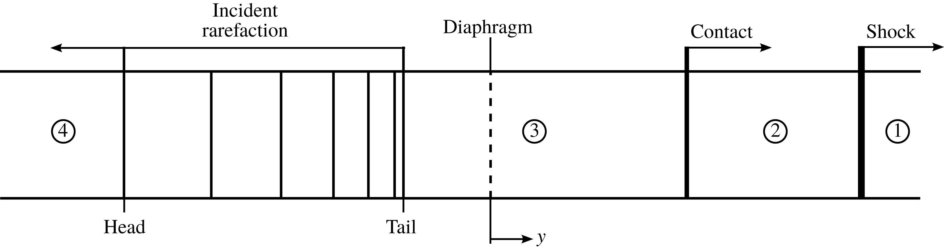
Before further investigation, one-dimensional inviscid shock tube theory is reviewed. In a typical single-phase shock tube, a diaphragm separates a high pressure (driver) and a low pressure (driven) section. When the diaphragm ruptures, there are traditionally four well-defined states as shown in figure 1 (Oosthuizen & Carscallen Reference Oosthuizen and Carscallen2013). The states are separated by travelling waves that work to equilibrate the pressure in the tube. These waves include a shock and contact wave that travel toward the driven section. Additionally, a rarefaction wave moves into the driver section. States 1 and 4 correspond to the original undisturbed driven and driver portions of the shock tube, respectively. After the diaphragm bursts, the region between the tail of the rarefaction wave and the moving shock is called the star region. In the star region, the pressure and velocity are constant. Across the shock, all gas properties are discontinuous. A contact wave follows behind the shock. Unlike the shock, only the temperature and density of the gas are discontinuous across the contact. From this, it is seen that the star region consists of states 2 and 3, where state 2 is the region between the shock and contact and state 3 is the region between the contact and rarefaction tail. For given driver and driven initial conditions, one-dimensional inviscid conservation equations can be used to fully determine the properties in each of these states along with the relative wave speeds.
The standard states and their numbering are shown here for a one-dimensional shock tube.

As previously noted, multiphase shock tubes have been used to study the dynamics of volcanic eruptions. In doing this, particles are added to the driver portion of the shock tube (state 4). While the contact and shock move away from the particle bed, the incident rarefaction wave generated at the diaphragm interacts directly with the particle bed and causes the bed to swell and move in the same direction as the shock. The section below the diaphragm continues to depressurize as the pressure equilibrates in the tube. This process causes the particle bed to expand and become less dense and particle–particle interactions become less frequent.
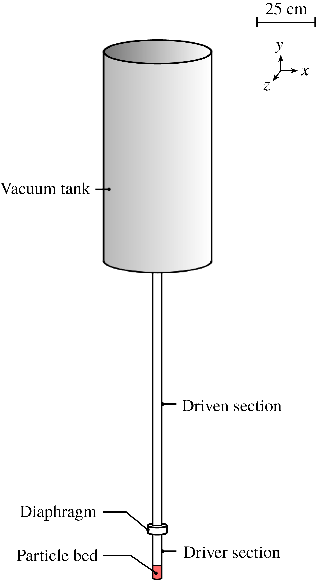
While there are several experiments to compare with, in this work the main experiments that we will use for comparison are those performed by Cagnoli et al. (Reference Cagnoli, Barmin, Melnik and Sparks2002). The experiments consist of a multiphase vertical air shock tube with particles at the bottom of the tube as shown in figure 2. The tube is divided into two smaller Pyrex™ sections of inner diameter 3.8 cm that are separated by a diaphragm. The gas inside both sections is air, which is initially at atmospheric conditions. A large vacuum tank that is approximately 50 cm in diameter and 1 m in height is connected to the driven tube. Compared to the horizontal shock tube in figure 1, in this vertical shock tube the lower section is the driver section and the upper section is the driven section. Spherical glass particles are used in this case as analogues to volcanic fragments. Before the start of each experiment, particles are poured into the driver portion of the tube by weight. The vacuum tank is then evacuated to a sub-atmospheric pressure. In doing this, the pressure difference between the driver and driven sections is increased. Once a desired pressure drop has been reached, the diaphragm is ruptured. Depending on the pressure difference and particle mass loading, the rapid depressurization and subsequent particle expansion will typically result in the ejection of particles from the shock tube into the vacuum tank. Although, for mild pressure differences the particles may be entirely contained within the shock tube.
Configuration for the experiments of Cagnoli et al. (Reference Cagnoli, Barmin, Melnik and Sparks2002).

While there have been multiple experimental studies that use multiphase shock tubes to understand the dynamics of volcanic eruptions, there have been few, if any, similar computational studies. The experiments reported in Cagnoli et al. (Reference Cagnoli, Barmin, Melnik and Sparks2002) are well suited for Euler–Lagrange simulations. The shock tube gas is air, which is accurately modelled as an ideal gas at the modest experimental pressures. The particle bed also consists of manufactured spherical glass particles with relatively uniform properties. When compared to other experiments, this is useful from a modelling perspective as other experiments may often use volcanic ash field samples that are composed of highly irregularly shaped particles (Alatorre-Ibargüengoitia et al. Reference Alatorre-Ibargüengoitia, Scheu, Dingwell, Delgado-Granados and Taddeucci2010).
In addition to the materials, the experiments of Cagnoli et al. (Reference Cagnoli, Barmin, Melnik and Sparks2002) present clear comparison metrics. In their experiments, the pressure drop across the diaphragm was varied. At each pressure drop, three similar experiments were run. During the simulation, the expanding particle bed front was tracked in time. After a short duration, the leading particle front moves at a near constant velocity. This velocity, called the bed front rise velocity, has been measured for each experiment and reported. In addition to the front rise velocity, high speed images were captured of the expanding particle bed at many different instances in time.
3 Governing equations and discretizations
In this section, the governing equations are presented for both the gas and the particle phases. It is noted that multiphase flow can often involve many different notations. For this reason, the notation used in the remainder of this work will be the following unless otherwise indicated. A subscript will be added when necessary to denote the fluid (gas) (
 $f$
) and the particle (
 $p$
) phases. Lower-case letters will refer to Eulerian field quantities while upper-case letters will refer to Lagrangian quantities. Finally, vectors and tensors will be denoted by bold letters. Note that the fluid velocity in the Eulerian reference frame will be denoted by
 $\boldsymbol{u}$
and the particle velocity in the Lagrangian reference frame will be denoted by
 $\boldsymbol{V}$
.
3.1 Gas equations
The governing gas equations are now presented in the Eulerian reference frame. For a general multiphase system, the governing equations are given by Ling, Balachandar & Parmar (Reference Ling, Balachandar and Parmar2016) for conservation of mass, momentum, and energy as
 $$\begin{eqnarray}\displaystyle & \displaystyle \frac{\unicode[STIX]{x2202}(\unicode[STIX]{x1D719}_{f}\unicode[STIX]{x1D70C}_{f})}{\unicode[STIX]{x2202}t}+\unicode[STIX]{x1D735}\boldsymbol{\cdot }(\unicode[STIX]{x1D719}_{f}\unicode[STIX]{x1D70C}_{f}\boldsymbol{u})=0, & \displaystyle\end{eqnarray}$$
 $$\begin{eqnarray}\displaystyle & \displaystyle \frac{\unicode[STIX]{x2202}(\unicode[STIX]{x1D719}_{f}\unicode[STIX]{x1D70C}_{f}\boldsymbol{u})}{\unicode[STIX]{x2202}t}+\unicode[STIX]{x1D735}\boldsymbol{\cdot }(\unicode[STIX]{x1D719}_{f}\unicode[STIX]{x1D70C}_{f}\boldsymbol{u}\boldsymbol{u}+\unicode[STIX]{x1D719}_{f}p\unicode[STIX]{x1D644})=p\unicode[STIX]{x1D735}\unicode[STIX]{x1D719}_{f}+\boldsymbol{f}_{pf}, & \displaystyle\end{eqnarray}$$
 $$\begin{eqnarray}\displaystyle & \displaystyle \frac{\unicode[STIX]{x2202}(\unicode[STIX]{x1D719}_{f}\unicode[STIX]{x1D70C}_{f}E_{f})}{\unicode[STIX]{x2202}t}+\unicode[STIX]{x1D735}\boldsymbol{\cdot }(\unicode[STIX]{x1D719}_{f}\unicode[STIX]{x1D70C}_{f}\boldsymbol{u}E_{f}+p\boldsymbol{u}_{m})=g_{pf}+q_{pf}. & \displaystyle\end{eqnarray}$$
In the above equations,
 $\unicode[STIX]{x1D70C}_{f}$
and
 $\unicode[STIX]{x1D719}_{f}$
are the density and volume fraction of the gas and
 $\unicode[STIX]{x1D719}_{p}$
is the volume fraction of the particulate phase (
 $\unicode[STIX]{x1D719}_{f}=1-\unicode[STIX]{x1D719}_{p}$
). Additionally,
 $\boldsymbol{f}_{pf}$
is the coupling force from the particles on the gas,
 $g_{pf}$
is the work done by that force,
 $p$
is the gas pressure and
 $E_{f}$
is the total energy of the gas per unit mass. Note that the stress tensor here is taken to be the isotropic component (pressure) as viscous effects in the bulk are ignored, since the inviscid forces dominate this compressible flow. Viscous effects due to inter-phase interactions are handled by the particle–gas coupling terms. In the energy equation, the mixture velocity
 $\boldsymbol{u}_{m}=\unicode[STIX]{x1D719}_{f}\boldsymbol{u}+\unicode[STIX]{x1D719}_{p}\boldsymbol{v}$
has been used where
 $\boldsymbol{u}$
and
 $\boldsymbol{v}$
are the Eulerian velocity vectors of the gas and the particles, respectively. Note that the direct heat exchange between the fluid and the particles
 $q_{pf}$
has been neglected here due to the modest shock tube pressures used in this work. These conservation equations are coupled through an equation of state for the gas. In this work, the equation of state is assumed to be that of a calorically perfect ideal gas, which can be written as
 $$\begin{eqnarray}p=\unicode[STIX]{x1D70C}_{f}(\unicode[STIX]{x1D6FE}-1)e_{f}=\unicode[STIX]{x1D70C}_{f}RT_{f},\end{eqnarray}$$
where
 $e_{f}=E_{f}-|\boldsymbol{u}|^{2}/2$
is the internal energy of the gas,
 $\unicode[STIX]{x1D6FE}$
is the ratio of specific heats,
 $R$
is the specific gas constant and
 $T_{f}$
is the temperature of the gas.
3.2 Particle equations
Following this, the governing particle equations are represented in the Lagrangian reference frame. Unless otherwise stated, it will be assumed that the particles in this work do not lose mass and are thermally equilibrated with the ambient fluid. This latter assumption is consistent with
 $q_{pf}=0$
. Therefore, the governing equations for each individual particle are the position evolution and conservation of momentum (velocity evolution) equations, which are given by
 $$\begin{eqnarray}\displaystyle & \displaystyle \frac{\text{d}\boldsymbol{X}}{\text{d}t}=\boldsymbol{V}, & \displaystyle\end{eqnarray}$$
 $$\begin{eqnarray}\displaystyle & \displaystyle M_{p}\frac{\text{d}\boldsymbol{V}}{\text{d}t}=\boldsymbol{F}_{qs}+\boldsymbol{F}_{un}+\boldsymbol{F}_{b}+\boldsymbol{F}_{c}, & \displaystyle\end{eqnarray}$$
respectively (Balachandar & Eaton Reference Balachandar and Eaton2010; Ling et al.
Reference Ling, Wagner, Beresh, Kearney and Balachandar2012, Reference Ling, Balachandar and Parmar2016). Here,
 $\boldsymbol{X}$
,
 $\boldsymbol{V}$
and
 $M_{p}$
are the position, velocity and mass of each particle in the Lagrangian reference frame. The terms on the right-hand side of the velocity evolution equation are the momentum forcing terms. The vectors
 $\boldsymbol{F}_{qs}$
and
 $\boldsymbol{F}_{un}$
are the quasi-steady and undisturbed flow forces which comprise the total hydrodynamic force contribution to each particle. Additionally,
 $\boldsymbol{F}_{b}$
is an external body force applied to each particle and
 $\boldsymbol{F}_{c}$
is the net collisional force on the particle, due to its interaction with other neighbouring particles and nearby obstacles.
There are different choices to model the quasi-steady force. Here, we have employed a general framework so that the quasi-steady force is given by
 $$\begin{eqnarray}\boldsymbol{F}_{qs}=\unicode[STIX]{x1D6FD}V_{p}(\boldsymbol{U}-\boldsymbol{V}),\end{eqnarray}$$
where
 $V_{p}$
is the volume of an individual particle,
 $\boldsymbol{U}$
is the gas velocity at the particle’s location and
 $\unicode[STIX]{x1D6FD}$
is the drag coefficient given by an individual drag model. This coefficient often involves the particle Reynolds number
 $Re_{p}=|\boldsymbol{U}-\boldsymbol{V}|\unicode[STIX]{x1D70C}_{f}D_{p}/\unicode[STIX]{x1D707}_{f}$
, particle Mach number
 $Ma_{p}=|\boldsymbol{U}-\boldsymbol{V}|/a_{f}$
and the local particle volume fraction
 $\unicode[STIX]{x1D719}_{p}$
. Here, the gas dynamic viscosity is
 $\unicode[STIX]{x1D707}_{f}$
,
 $D_{p}$
is the diameter of a particle and
 $a_{f}$
is the local speed of sound in the gas. Note that
 $\unicode[STIX]{x1D6FD}$
is often highly nonlinear and its functional form is theoretically motivated but empirically fit. Unless otherwise noted, the drag force will be modelled as that of a fluidized bed through the Gidaspow drag correlation (Gidaspow Reference Gidaspow1994). This empirical model is given by
 $$\begin{eqnarray}\unicode[STIX]{x1D6FD}=\left\{\begin{array}{@{}ll@{}}150{\displaystyle \frac{\unicode[STIX]{x1D719}_{p}}{\unicode[STIX]{x1D719}_{f}}}{\displaystyle \frac{\unicode[STIX]{x1D707}_{f}}{D_{p}^{2}}}+1.75{\displaystyle \frac{\unicode[STIX]{x1D70C}_{f}}{D_{p}}}|\boldsymbol{U}-\boldsymbol{V}|,\quad & \unicode[STIX]{x1D719}_{p}>0.2,\\ 0.75C_{D}^{\ast }{\displaystyle \frac{\unicode[STIX]{x1D719}_{f}}{D_{p}}}\unicode[STIX]{x1D70C}_{f}|\boldsymbol{U}-\boldsymbol{V}|\unicode[STIX]{x1D719}_{f}^{-2.65},\quad & \unicode[STIX]{x1D719}_{p}\leqslant 0.2,\end{array}\right.\end{eqnarray}$$
where the drag coefficient
 $C_{D}^{\ast }$
is based on the volume weighted Reynolds number
 $Re_{p}^{\ast }=\unicode[STIX]{x1D719}_{f}Re_{p}$
and given by
 $$\begin{eqnarray}C_{D}^{\ast }=\left\{\begin{array}{@{}ll@{}}{\displaystyle \frac{24}{Re_{p}^{\ast }}}(1+0.15(Re_{p}^{\ast })^{0.687}),\quad & Re_{p}^{\ast }\leqslant 10^{3},\\ 0.44,\quad & Re_{p}^{\ast }>10^{3}.\end{array}\right.\end{eqnarray}$$
While the Gidaspow drag model has traditionally been used at much lower velocities than are initially seen in a shock tube, the relative velocities in and around the particle bed are orders of magnitude smaller after the incident rarefaction wave has initially impacted the bed. Furthermore, the Gidaspow drag model has been used with success even in cases where the shock propagates directly over higher concentrations of particles (Shallcross & Capecelatro Reference Shallcross and Capecelatro2018).
In addition to the quasi-steady force, the undisturbed force is given by
 $$\begin{eqnarray}\boldsymbol{F}_{un}=-V_{p}\unicode[STIX]{x1D735}P,\end{eqnarray}$$
where
 $\unicode[STIX]{x1D735}P$
refers to the gas pressure gradient evaluated at each particle’s location. Particles also receive an external body force due to the gravitational acceleration on each particle, resulting in
 $$\begin{eqnarray}\boldsymbol{F}_{b}=M_{p}\boldsymbol{g},\end{eqnarray}$$
where
 $\boldsymbol{g}$
is the gravitational acceleration. Due to the large density difference between the gas and particles, the buoyancy force can be ignored. Lastly, particle–particle and particle–wall collisional forces are handled through a soft-sphere spring-damper collision model, similar to the one originally proposed by Cundall & Strack (Reference Cundall and Strack1979). For the
 $i$
th particle, the normal collision force from each overlapping
 $j$
th particle is computed by
 $$\begin{eqnarray}\boldsymbol{F}_{c,ij}=-k_{c}\unicode[STIX]{x1D6FF}_{ij}\boldsymbol{n}_{ij}-\unicode[STIX]{x1D702}\boldsymbol{V}_{ij},\end{eqnarray}$$
where
 $k_{c}$
is the normal spring stiffness parameter,
 $\unicode[STIX]{x1D6FF}_{ij}$
is the relative overlap between colliding particles,
 $\boldsymbol{n}_{ij}$
is the unit vector from the centre of particle
 $i$
to the centre of particle
 $j$
,
 $\unicode[STIX]{x1D702}$
is the normal damping coefficient and
 $\boldsymbol{V}_{ij}$
is the normal relative contact velocity. The damping coefficient is a function of the spring stiffness, mass of colliding particles, and normal coefficient of restitution
 $e_{n}$
. Thus, the two model parameters controlling collision strength and dissipation are
 $k_{c}$
and
 $e_{n}$
. After each individual collision force has been accounted for, the total collision force on a particle
 $\boldsymbol{F}_{c}$
is the sum of all collisions with each overlapping
 $j$
th particle. Note that collisions with walls are handled in this model by assuming the wall to be a particle of infinite mass and zero diameter. For further details on this model see Zwick & Balachandar (Reference Zwick and Balachandar2019).
3.3 Gas discretization
In order to solve the governing equations for the gas, we have extended the single-phase discontinuous Galerkin spectral element method (DG-SEM) of Hackl et al. (Reference Hackl, Shringarpure, Koneru, Delchini and Balachandarsubmitted) to include the aforementioned multiphase components. The extension of the DG-SEM methodology from the single-phase governing equations to the multiphase equations found in (3.1), (3.2) and (3.3) requires three steps. The first step is projection of specific particle quantities onto the Eulerian reference frame. Note that the process of projection is described in the next section and results in the Eulerian fields
 $\unicode[STIX]{x1D719}_{f}$
,
 $\unicode[STIX]{x1D719}_{p}$
,
 $\boldsymbol{f}_{pf}$
,
 $g_{pf}$
and
 $\unicode[STIX]{x1D719}_{p}\boldsymbol{v}$
, which in turn are needed in the evolution of the gas phase properties. After obtaining the fluid volume fraction, the second step requires multiplication of the original conserved variables and fluxes by the fluid volume fraction. Lastly, the right-hand side of (3.1), (3.2) and (3.3) are added as source terms in the governing equations. From this, it is noted that the fluid solver itself has not been modified since the conserved variables and fluxes have only been multiplicatively altered. All other multiphase terms are added as volumetric source terms. Thus, the original DG-SEM implementation of Hackl et al. (Reference Hackl, Shringarpure, Koneru, Delchini and Balachandarsubmitted) has been used and is now briefly described.
The entire simulation domain is broken into hexahedral spectral elements (Deville, Fischer & Mund Reference Deville, Fischer and Mund2002) that span the entire domain. The nodal discontinuous Galerkin method (Hesthaven & Warburton Reference Hesthaven and Warburton2008) is applied within each element. For each elemental domain, the conservation equations are solved in the weak form by invoking the Galerkin statement that both the solution and the test function are approximated by the same basis expansion. The solution to the system of equations (3.1), (3.2) and (3.3) is the conserved variables at each grid point, so that the solution may be written as
 $\boldsymbol{u}_{c}=(\unicode[STIX]{x1D719}_{f}\unicode[STIX]{x1D70C}_{f},\unicode[STIX]{x1D719}_{f}\unicode[STIX]{x1D70C}_{f}u,\unicode[STIX]{x1D719}_{f}\unicode[STIX]{x1D70C}_{f}v,\unicode[STIX]{x1D719}_{f}\unicode[STIX]{x1D70C}_{f}w,\unicode[STIX]{x1D719}_{f}\unicode[STIX]{x1D70C}_{f}E_{f})$
, where
 $\boldsymbol{u}=(u,v,w)$
. Then, the solution is approximated by a series expansion of the Lagrange polynomials
 $$\begin{eqnarray}\boldsymbol{u}_{c}(\boldsymbol{x})\approx \mathop{\sum }_{k=1}^{N}\mathop{\sum }_{j=1}^{N}\mathop{\sum }_{i=1}^{N}\hat{\boldsymbol{u}}_{c,i,j,k}L_{i}(x)L_{j}(y)L_{k}(z),\end{eqnarray}$$
where the
 $i$
th Lagrange polynomial is
 $$\begin{eqnarray}L_{i}(x)=\mathop{\prod }_{q=1,q\neq i}^{N}\frac{(x-x_{q})}{(x_{i}-x_{q})},\end{eqnarray}$$
and similarly for the
 $y$
and
 $z$
directions. Note that the coefficients
 $\hat{\boldsymbol{u}}_{c,i,j,k}$
are now the unknowns in the system. Since Lagrange polynomials are used, the unknowns correspond to
 $\boldsymbol{u}_{c}$
collocated at the grid points. Recall that the solution is expressed on each local elemental basis. Each element contains a sub-elemental resolution that utilizes the clustered Legendre–Gauss–Lobatto (GLL) points, where in one-dimension,
 $x_{i}$
are the
 $N$
GLL points that satisfy
 $P_{N-1}^{\prime }|_{x=x_{i}}=0$
, where
 $P_{N-1}(x)$
is the
 $N-1$
associated Legendre polynomial. Similarly, the GLL weights
 $w_{i}$
are defined as
 $$\begin{eqnarray}w_{i}=\left\{\begin{array}{@{}ll@{}}{\displaystyle \frac{2}{N(N-1)}},\quad & i=1,\ldots ,N,\\ {\displaystyle \frac{2}{N(N-1)[P_{N-1}(x_{i})]^{2}}},\quad & \text{otherwise}.\end{array}\right.\end{eqnarray}$$
Note that the grid resolution
 $N$
has been introduced, which corresponds to the number of unidirectional GLL grid points within each element. Now, for a given field
 $f(r,s,t)$
, integrals can discretely be written in the following form:
 $$\begin{eqnarray}F=\int _{-1}^{1}\int _{-1}^{1}\int _{-1}^{1}f(r,s,t)\,\text{d}r\,\text{d}s\,\text{d}t\approx \mathop{\sum }_{k=1}^{N}\mathop{\sum }_{j=1}^{N}\mathop{\sum }_{i=1}^{N}w_{i}w_{j}w_{k}\,f(r_{i},s_{j},t_{k}).\end{eqnarray}$$
This quadrature approximation is exact for polynomials up to
 $2N-3$
. The bounds on the integrals imply that each element has a mapping to go from its original spatial extent in the
 $x,y,z$
coordinates to a reference unit element in the
 $r,s,t$
coordinates. The reference element is a non-skewed element whose spatial extent is in
 $r,s,t\in [-1,1]$
. The discrete system of conserved variables at each GLL grid point is then advanced in time using a third-order Runge–Kutta method.
Finally, while not shown here, entropy bounded artificial mass, momentum and energy diffusion have been added as source terms in the governing equations to stabilize the Galerkin method around discontinuities. In this work, we follow Hackl et al. (Reference Hackl, Shringarpure, Koneru, Delchini and Balachandarsubmitted) by using their artificial viscosity implementation which has been set according to their recommendation.
3.4 Particle discretization
The key computational steps in the particle solution can be summarized by Zwick & Balachandar (Reference Zwick and Balachandar2019): (i) interpolation of fields from the grid points to each particle’s location, (ii) time advancement of each particle’s position and velocity using (3.5) and (3.6), (iii) projection of particle quantities to the surrounding grid points and (iv) collision detection between neighbouring particles.
Given a field with discrete values at each GLL grid point, interpolation is computed by evaluating a field’s Lagrange polynomial representation at the off-grid locations of each particle. Since the GLL grid is defined on an element-by-element basis, interpolation only requires the values of interpolated fields of the element that a particle is in. Clever factorization of Lagrange interpolation, called barycentric Lagrange interpolation, is used which only requires
 $O(N^{3})$
operations for spectrally accurate interpolation of each particle (Berrut & Trefethen Reference Berrut and Trefethen2004). Once the required fields have been interpolated, the particle force models found on the right-hand side of (3.5) and (3.6) are evaluated. The system of equation is then advanced in time using a third-order Runge–Kutta method.
In the third step, particle quantities are projected to the surrounding grid points. Projection can be thought of as the inverse of interpolation and consists of evaluating a kernel, which in this case is a normalized Gaussian function, whose centre coincides with the position of the particle. Different Lagrangian quantities are projected which results in an Eulerian field for each projected quantity. Table 1 represents the Eulerian field variable
 $a(\boldsymbol{x})$
that results from the projection of the Lagrangian quantity
 $A(\boldsymbol{X})$
. For
 $N_{p}$
total particles, projection of the Lagrangian quantity to the Eulerian field is computed by
 $$\begin{eqnarray}a(\boldsymbol{x})=\mathop{\sum }_{i=1}^{N_{p}}A_{i}(\boldsymbol{X})g_{{\mathcal{M}}}(\boldsymbol{x}-\boldsymbol{X}),\end{eqnarray}$$
where
 $g_{{\mathcal{M}}}$
is a Gaussian function. In this way, projection can be equated with a filtering operation. Thus, the Gaussian function is characterized by a filter half-width
 $\unicode[STIX]{x1D6FF}_{f}$
, which is a measure of how many local grid points a projected particle quantity will spread over relative to its position. This is used in conjunction with the Eulerian mesh spacing
 $\unicode[STIX]{x1D6E5}$
and particle diameter to define the two non-dimensional parameters
 $\unicode[STIX]{x1D6FF}_{f}/\unicode[STIX]{x1D6E5}$
and
 $\unicode[STIX]{x1D6FF}_{f}/D_{p}$
(Zwick & Balachandar Reference Zwick and Balachandar2019). In table 1,
 $G_{pf}$
is the work done by the particle–gas hydrodynamic force
 $\boldsymbol{F}_{pf}$
and the negative signs have been added due to Newton’s third law to account for the back influence on the gas phase (Ling et al.
Reference Ling, Balachandar and Parmar2016). In this work, the work done by the undisturbed flow force is included implicitly while the work done by the quasi-steady force is not considered. While the quasi-steady force’s energy contribution will undoubtedly be important in more extreme compressible flows, its effects are of secondary importance for the milder conditions under investigation. In the present formulation the hydrodynamic coupling force is the quasi-steady contribution, so that
 $\boldsymbol{F}_{pf}=\boldsymbol{F}_{qs}$
.
Parameters used in projection.

The last computationally intensive step is in collision detection. From (3.12) it is observed that every
 $i$
th particle may collide with every other
 $j$
th particle. Such a search for all possible collisions may be prohibitively expensive as this scales as
 $O(N_{p}^{2})$
collision checks, where
 $N_{p}$
is the number of particles. While not discussed here, this cost is significantly reduced through the binned ghost particle algorithm (Zwick & Balachandar Reference Zwick and Balachandar2019). When two particles overlap, they each receive a spring-damper force which is governed by the spring stiffness
 $k_{c}$
and the coefficient of restitution
 $e_{n}$
. For more details on the particle solver and its implementation, see Zwick (Reference Zwick2019a
).
4 Physical regime classification
We now turn our attention to classification of the underlying physics. While there have been attempts to classify these flow regimes experimentally, these classifications have not been detailed. In particular, classification of experimental results have typically been exploratory in nature (Anilkumar Reference Anilkumar1989). In the remainder of this work, we aim to reconcile the observed physical phenomena from analysis of our simulations. In pursuit of this goal, three cases at different pressure ratios across the diaphragm have been simulated in three-dimensions. In this section, we first begin by describing the set-up of the simulations. Then, we provide a regime map from the simulations to illustrate the partitioning between different physical regimes that have been observed. Each regime is then more thoroughly detailed and the simulations are compared to the accompanying experiments.
4.1 Simulation set-up
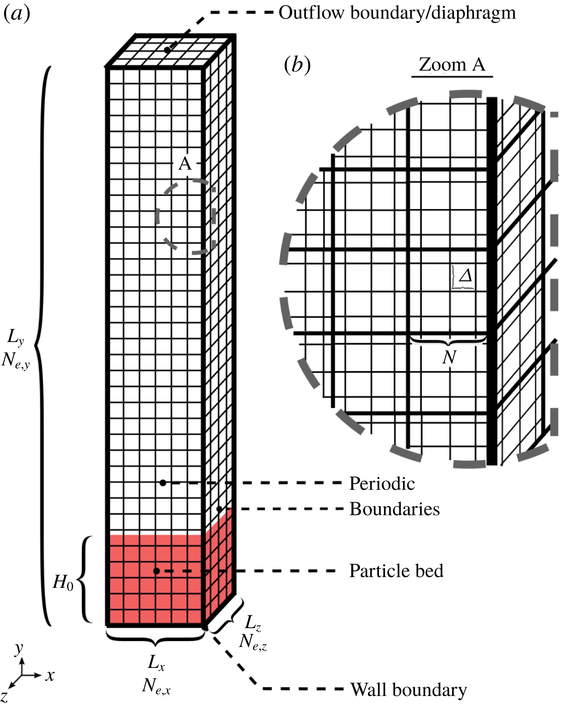
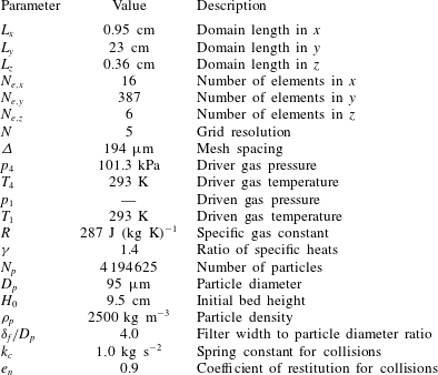
The set-up for the present simulations is shown in figure 3. The parameters are meant to mimic those of experimental set Q of Cagnoli et al. (Reference Cagnoli, Barmin, Melnik and Sparks2002). Here, we are only simulating the portion of the shock tube below the diaphragm. Additionally, in this work we are not concerned with the effects of the shock tube geometry on the flow. The reason for this is that we seek to understand how the particle–fluid and particle–particle coupling mechanisms lead to various phenomena in and around the particle bed in the absence of geometric constraints. Instead of the experimental vertical side walls, periodic boundary conditions have been used in the simulation resembling a domain of infinite width. Thus, although the simulation domain appears to have a rectangular cross-section, the resulting features are expected to be isotropic due to periodicity. Our simulations can be characterized by the fluid and particle parameters depicted in figure 3 and described in table 2.
Schematic of simulation domain. In (a), the spectral elements are shown. In (b), a zoomed section is given which shows the sub-element GLL grid within each element. The boundary conditions are also given in the figure.

Description of simulation parameters and their values.

Here, the domain is of length
 $L_{x}$
,
 $L_{y}$
,
 $L_{z}$
in the
 $x,y,$
and
 $z$
directions. In each direction there are
 $N_{e,x}$
,
 $N_{e,y}$
, and
 $N_{e,z}$
elements. The sub-elemental GLL grid resolution is given by
 $N$
. Due to the non-uniform nature of the GLL grid points, the actual mesh spacing
 $\unicode[STIX]{x1D6E5}$
is computed from the element spacing and the GLL resolution and represents the average spacing between grid points within each element (Beyer Reference Beyer1987). In this work, the element spacing, which is computed by the domain length divided by the number of elements in each direction is equal so that the mesh spacing is the same in each direction. Prior to the diaphragm burst, the temperature of the gas is kept at ambient conditions
 $T_{4}=T_{1}$
. The driver section is held at ambient pressure
 $p_{4}$
while the driven section is evacuated to a lower pressure
 $p_{1}$
. Three different driven pressures are used in this work, which are
 $p_{1}=71.3$
, 51.3 and 31.3 kPa which correspond to cases F1, F2 and F3, respectfully. Additionally, the gas used is air, which has the specific gas constant
 $R$
and specific heat ratio
 $\unicode[STIX]{x1D6FE}$
given in the table. The particle bed of initial height
 $H_{0}$
is composed of monodisperse spherical particles of diameter
 $D_{p}$
and density
 $\unicode[STIX]{x1D70C}_{p}$
.
Extensive two-dimensional simulations of this problem set-up using the Euler–Lagrange method have been studied (Zwick Reference Zwick2019b
). Simulations were carried out to detail the sensitivity of the results to various numerical and modelling parameters in the coupled gas–particle equations. From the two-dimensional results, reasonable values for the projection filter width
 $\unicode[STIX]{x1D6FF}_{f}$
and collisional parameters
 $k_{c}$
and
 $e_{n}$
were chosen and are presented in table 2.
In the simulations the initial conditions are specified for both the gas and the particle phases. The initial conditions for the gas phase can be thought of as specifying values for the conserved variables
 $\unicode[STIX]{x1D719}_{f}\unicode[STIX]{x1D70C}_{f}$
,
 $\unicode[STIX]{x1D719}_{f}\unicode[STIX]{x1D70C}_{f}\boldsymbol{u}$
and
 $\unicode[STIX]{x1D719}_{f}\unicode[STIX]{x1D70C}_{f}E_{f}$
. The gas density, velocity and total energy are computed at the instant directly before the rarefaction head hits the particle bed through NUMERICA, which is a library that uses an exact Riemann solver to obtain the initial shock tube gas states (Toro Reference Toro1999). The inputs to NUMERICA are the initial driver and driven section pressures and densities and the diaphragm position. Using the outputs from NUMERICA and the ideal gas law, the initial gas density, velocity, and total energy are obtained in the simulation domain. Note that the position of the diaphragm corresponds to the simulation outflow boundary. The implementation of the outflow boundary is such that it mimics a driven section of infinite length. Thus, the outflow is initially at the shock tube star state 3 (figure 1) since both the incident rarefaction head and tail travel down the shock tube in this work. At later times, the gas properties at the outflow (pressure, density, velocity, etc.) will change due to the incident rarefaction wave interacting with the particle bed.
The initial positions of the particles in the particle bed are obtained through a pre-simulation in which particles are randomly distributed in the entire domain and allowed to settle. After the particles have come to rest, the uppermost portion of the bed is removed so that the experimental bed height
 $H_{0}$
is matched and the initial bed front is flat. The generated particle bed is then used as the initial condition for the simulation. As previously noted, projection of each particle’s volume results in the particle volume fraction field
 $\unicode[STIX]{x1D719}_{p}$
which is used to compute the gas volume fraction
 $\unicode[STIX]{x1D719}_{f}=1-\unicode[STIX]{x1D719}_{p}$
. The gas volume fraction is then multiplied to the gas density, velocity and total energy from NUMERICA to complete the initial conditions of the conserved gas variables. Following initialization, the governing equations are advanced in time.
4.2 Regime map
From the results of the simulations, we observe multiple regimes of interest. In order to describe these regimes, we have put together a typical position versus time wave diagram of our results in figure 4. In the figure, only the most prominent waves and regimes are shown. Note that there may be additional waves that are weaker and therefore are not pictured here. Figure 4 provides a reasonable starting point for better understanding the physical processes at work.
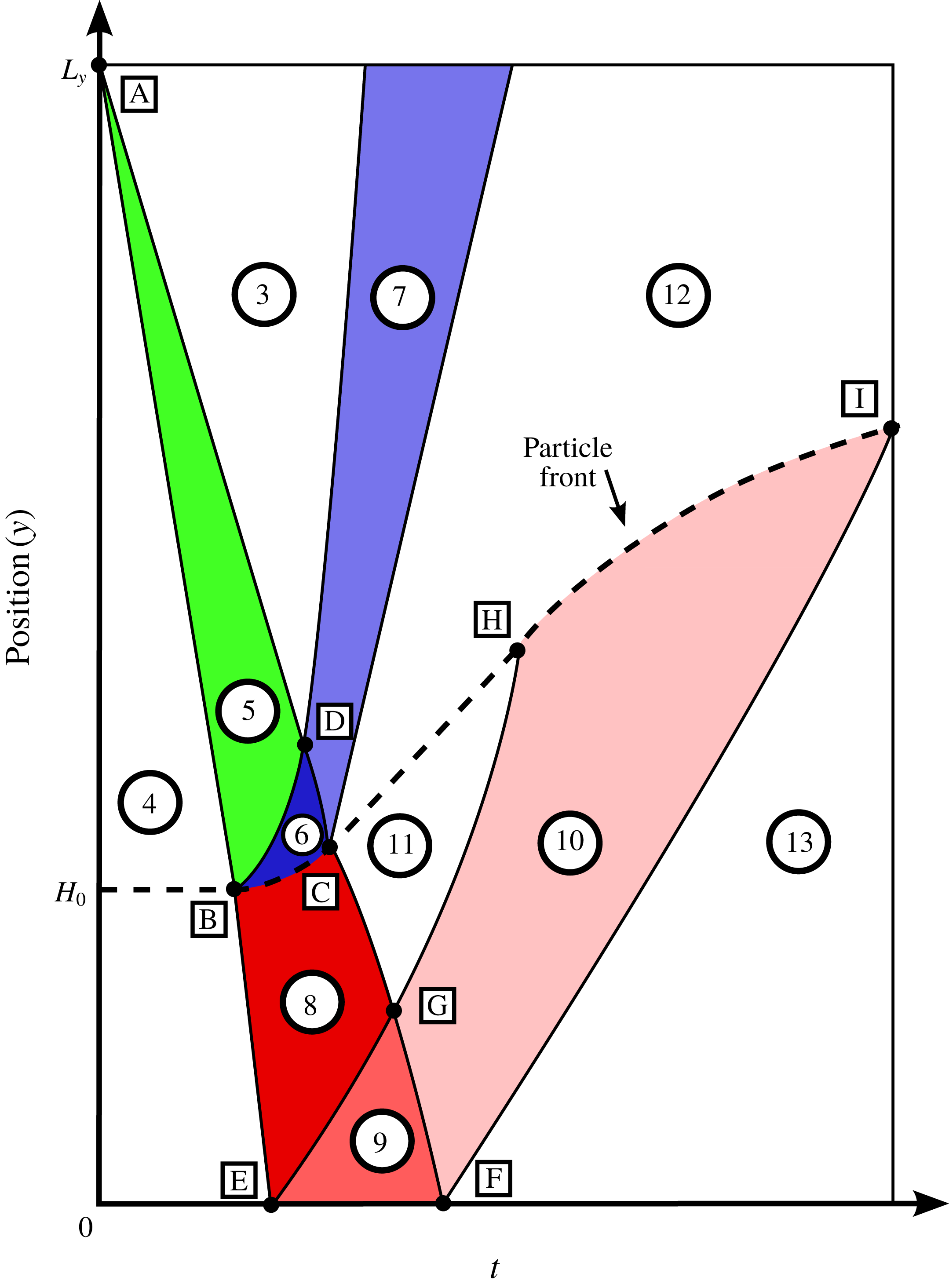
A model position versus time wave diagram for the present simulations. The numbers and letters here denote the shaded regimes and intersection points, respectively. The dashed line demarcates the particle front, with a particle–gas mixture below the line and only gas above the line. The colours denote the incident rarefaction waves (green), reflected rarefaction waves at the particle front (blue) and transmitted rarefaction waves into the bed (red).

In figure 4, the dashed line shows the particle front position as a function of time. Above the dashed line is entirely gas, while below the line is gas–particle mixture. The diaphragm is initially positioned at point A and the instant the diaphragm is burst is the reference point from which later times are measured. The diaphragm burst initiates the incident rarefaction wave in regime 5 (coloured green in the figure). The initial driver section and star states are regimes 4 and 3, respectively. The particle bed is first impacted by the rarefaction head at point B. At this instant, the incident rarefaction head is both transmitted and reflected from the particle bed. The transmitted head will reach the bottom wall at point E while the reflected rarefaction head will travel through the entire incident rarefaction wave packet and exit at point D. The incident rarefaction tail will accelerate once it sees the reflected waves travelling away from the particle bed and eventually impact the bed at point C. Similar to the incident rarefaction head, the tail will be both reflected and transmitted at the bed surface. Points B, C and D form regime 6 where the particle front accelerates from rest to a near constant velocity. After leaving regime 6, the reflection of the incident rarefaction wave form regime 7 as it travels back toward the diaphragm. In regime 8, the particle bed expands from both the particle front acceleration and the incident rarefaction wave transmission into the bed. When the particle front stops accelerating, the particle front and the gas just above the front travel at a constant velocity. In this state, the mixture in the upper portion of the bed forms regime 11 while above the bed is regime 12. In regime 10, the particle bed will see reflections off the bottom wall from the waves that were originally transmitted into the bed. Similar to the incident reflection from the top of the bed, the reflection from the bottom wall will accelerate the head from point E to point G and the tail from point G to point F. The waves reflected from the bottom wall make up regimes 9 and 10. Note that this is a more simplified view of the reflection from the bottom wall. In reality, the reflection at the bottom wall is more complicated since the bed is already moving. Due to this, there are characteristics of a reflected rarefaction in regimes 9 and 10 but their appearance is non-traditional when compared to a gas only case. Finally, the tail of the transmitted wave will reflect off the bottom wall at point F and eventually travel up into the expanding bed until it hits the front at point I. This demarcates the final regime 13, where the mixture has seen both the transmission of the incident rarefaction wave and its subsequent reflection from the bottom wall.
In order to arrive at the diagram in figure 4, we have numerically generated similar wave diagrams from each simulation. As it is customary in compressible flow simulation, we have used a synthetic Schlieren image generated through visualization of the gas density gradients to visualize the different waves (Haselbacher et al.
Reference Haselbacher, Balachandar and Kieffer2007). The first step is computing the fluid density gradient magnitude at every grid point. Then, the mean density gradient magnitude in every
 $x$
–
 $z$
plane along the simulation domain is evaluated. This is done at every simulation output time so that a position versus time contour plot of the density gradient magnitude can be produced. The simulation Schlieren images are shown for the three cases in figure 5.
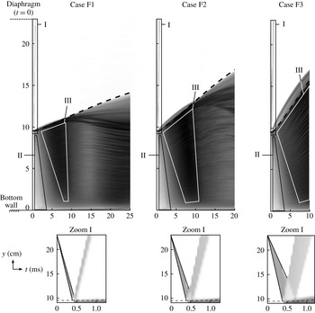
Numerical wave position versus time diagram. The diagram has been generated by evaluating the mean density gradient magnitude
 $\bar{|\unicode[STIX]{x1D735}\unicode[STIX]{x1D70C}_{f}|}$
in each
 $x$
–
 $z$
plane at every position and time in the domain. The grey-scale contours are coloured according to
 $\log _{10}\bar{|\unicode[STIX]{x1D735}\unicode[STIX]{x1D70C}_{f}|}$
with bounds of
 $-1$
(pure white) and 3 (pure black). A zoomed portion of region I at early times is also shown below each case. The dashed line in each case shows the highest particle’s trajectory in time so that below the line is a gas–particle mixture and above the line is entirely gas.

In figure 5, the incident rarefaction wave is seen in the zoomed views of region I in the bottom row and each wave is bounded by the two solid lines. The left line is the incident rarefaction head which has been plotted until
 $t_{B}$
, which is when it first impacts the particle bed. The right line is slower and corresponds to the incident tail and is plotted until
 $t_{D}$
, which is when the reflected incident head has reached the incident tail. Note that later, an estimate for
 $t_{D}$
is given. The reflected rarefaction wave is also seen in the zoomed region I figures, with their thickness increasing for increased pressure difference. In the upper figures, there also appears to be a large density gradient ahead of the particle front (demarcated by the dashed line) which grows initially and is more pronounced with increasing pressure differences. However, after some time this feature disappears. Inside the particle bed, large density gradients are observed. The larger gradients originate at the top of the bed and propagate into the interior of the bed as time increases.
While the transmission of the incident rarefaction wave is not as clear as its reflection, there are similarities between the three cases. The first is that the early transmitted wave inside the bed at times less than approximately 2–3 ms appears the same between cases as illustrated in region II. This is likely because the initial states below the diaphragm are the same between each case. Due to this, the incident rarefaction head initially travels at speed
 $a_{4}$
until it encounters the particle front, where it is then transmitted into the bed at the frozen sound speed. Thus, irrespective of pressure ratio, sound propagates at the same speed both inside and outside the bed. Secondly, after the front stops accelerating around 2–3 ms, the highest density gradients, which are the darkest colours, are observed in each case in region III. These high gradients persist until later times with increasing pressure ratio, as is seen from case F1 to F2. In case F3, there has not been enough time simulated to see this trend but we speculate that it continues at later times. While they appear smooth, the high density gradients in region III are composed of streaks of both high and lower density gradients. This is from the fluctuations in fluid density as the flow passes between voids and more densely packed regions of the bed. Due to this, bulk changes to the streamwise density gradient are difficult to detect at later times.
Position versus time diagrams for case F1. The contours correspond to mean values in each
 $x$
–
 $z$
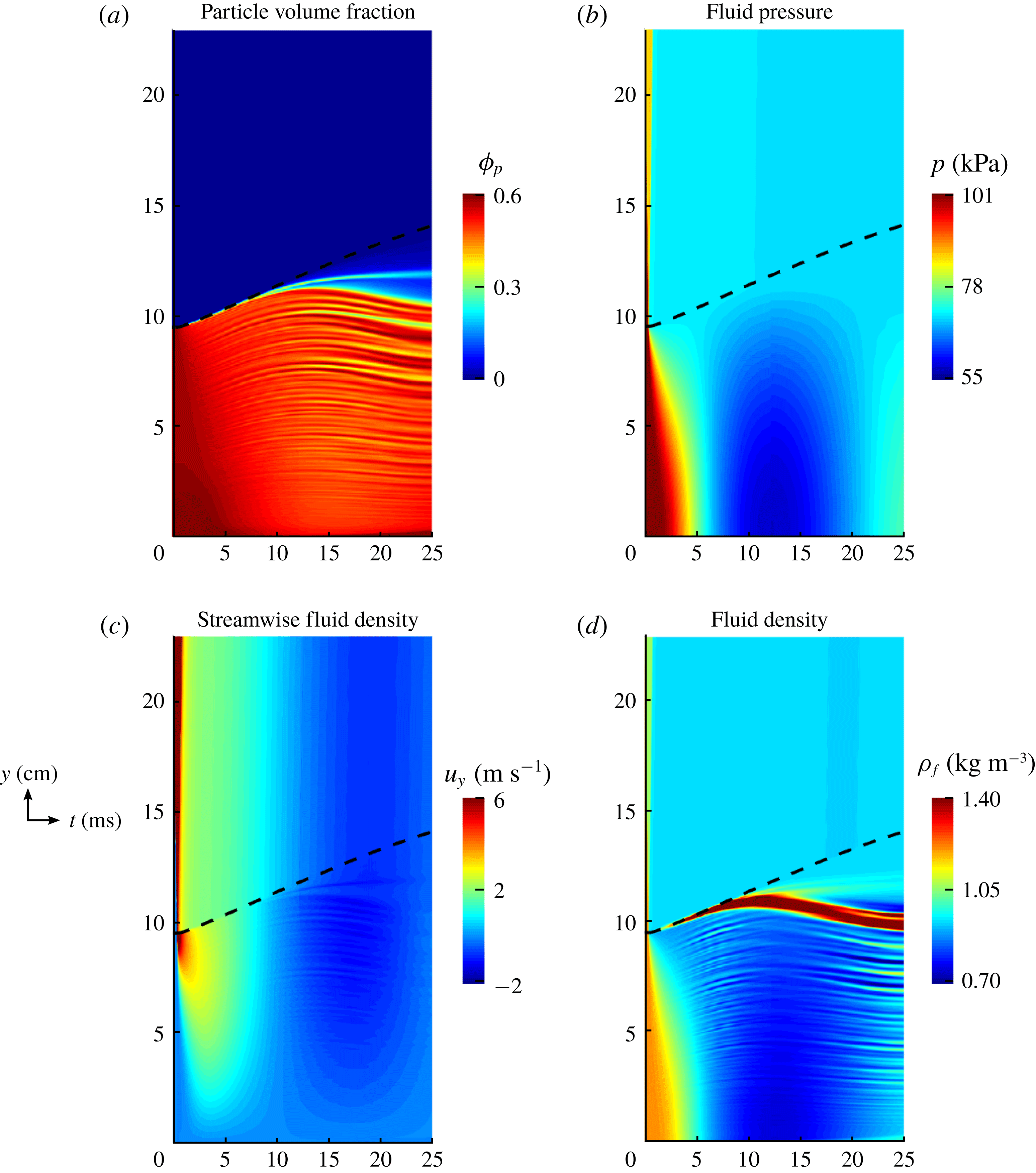
plane of each property. The dashed line in each case shows the highest particle’s trajectory in time so that below the line is a gas–particle mixture and above the line is entirely gas. (a) Particle volume fraction, (b) fluid pressure, (c) streamwise fluid velocity and (d) fluid density.

We have produced similar position versus time diagrams for the particle volume fraction, fluid pressure, streamwise fluid velocity and fluid density. The position versus time contours for case F1 are shown in figure 6. In the figure, there are many interesting characteristics that are observed. From the volume fraction contours, there are streaks of both low and high volume fractions which disappear and reappear within the bed. This happens even when initially there appears to be little variation in the original packing. Additionally, there is a very dilute region of particles which forms at late times at the top portion of the bed. Regarding the fluid pressure, a near constant low pressure is observed at the front of the bed after the front has accelerated. This initial drop in pressure occurs within a millisecond after the incident rarefaction head has impacted the bed. This finding is in agreement with the exponential pressure decay model of McGuinness & Singh (Reference McGuinness and Singh2015). At late times, an extremely low pressure is observed at the base of the bed which reaches its minimum value at approximately 12.5 ms. Interestingly, this low pressure is approximately 55 kPa and is the lowest pressure in the entire shock tube, being even lower than the original driven section pressure of 71 kPa in this case. It also appears that while the density gradient magnitude was sensitive to the voids present in the bed, the transmitted rarefaction wave (regimes 9 and 10 from figure 4) are more clearly seen in the pressure contours in figure 6(b). The reflection occurs after the mean pressure inside the bed is nearly constant around 6 ms. The pressure at the bottom of the bed then begins to drop at a faster rate than the top of the bed indicating the reflection of a pressure wave. From the streamwise fluid velocity, we can see that a high fluid velocity initially penetrates the upper portion of the bed but soon diminishes as the mixture equilibrates. At late times, the velocity fluctuates between positive and negative values meaning that the flow eventually travels in the opposite direction of the originally generated flow. Finally, from the fluid density, there appears to be a large increase in fluid density at the top of the bed, even above that of the original driver section’s density. It is clear that there are also strong fluctuations in density inside the bed at moderate times which appear correlated with the fluctuations in particle volume fraction. As previously suggested, this leads to higher density gradients inside the particle bed which are not representative of the bulk wave interactions.
Using these position versus time regime maps along with the previous particle bed characterization methods, some of the more prominent characteristics of our simulations will be studied in more detail. To do this, we have broken the remaining sections into two broader categories: (i) particle front dynamics and (ii) interior bed dynamics. Each will be analysed in what follows.
4.3 Acceleration of the particle front
Since traditional shock tube theory already predicts regimes 3, 4 and 5, we first begin by studying regime 6. In this regime, the particle front is accelerated from rest at point B to a constant velocity at point C. The time of arrival of the incident rarefaction head at the particle bed location is
 $t_{B}$
and is easily computed as
 $$\begin{eqnarray}t_{B}=\frac{L_{y}-H_{0}}{a_{4}},\end{eqnarray}$$
where
 $a_{4}$
is the speed of sound in the driver section, which is constant for every case since the driver section is held at ambient conditions. However, the coordinates of point C are harder to determine due to the nonlinear reflections off the particle front.
The acceleration delivered to the particle bed in regime 6 has been estimated experimentally by Cagnoli et al. (Reference Cagnoli, Barmin, Melnik and Sparks2002). For the companion experiments to simulation case F1, the reported average acceleration was around
 $75g$
. This can also be estimated by dividing the front rise velocity by the time taken to accelerate to this velocity. From the experiments, this corresponds to the front being accelerated from 0 to approximately 1.7–
 $1.9~\text{m}~\text{s}^{-1}$
. Since this increase in velocity occurred over a window of 2.5 ms, average accelerations of
 $69g$
to
 $77g$
can reasonably be estimated. While these are unarguably large accelerations, the present simulations show that the instantaneous accelerations of particles at the front can be much higher.
This can be explained from consideration of an extreme case related to this flow. Consider a case where a single particle is initially placed at the location of the particle front relative to the diaphragm. However, in this simple example both the particle bed and the bottom wall are absent. In this case, the particle is assumed to be one-way coupled with the gas flow, meaning that it will not alter the ambient conditions and the flow will follow standard shock tube theory as presented in figure 1. Then, exactly at time
 $t_{B}$
after the diaphragm burst, the particle will be accelerated by the incident rarefaction wave and eventually enter the shock tube star region (regime 3) where the particle will eventually come to travel at the shock tube star velocity. This scenario can be also considered as the very dilute limit. This isolated particle has been numerically simulated for the conditions corresponding to case F1. For a fair comparison, the drag model is evaluated as if the single particle was in a bed of packed particles (
 $\unicode[STIX]{x1D719}_{p}\approx 0.64$
) as it would normally be. (We tested this assumption using different
 $\unicode[STIX]{x1D719}_{p}$
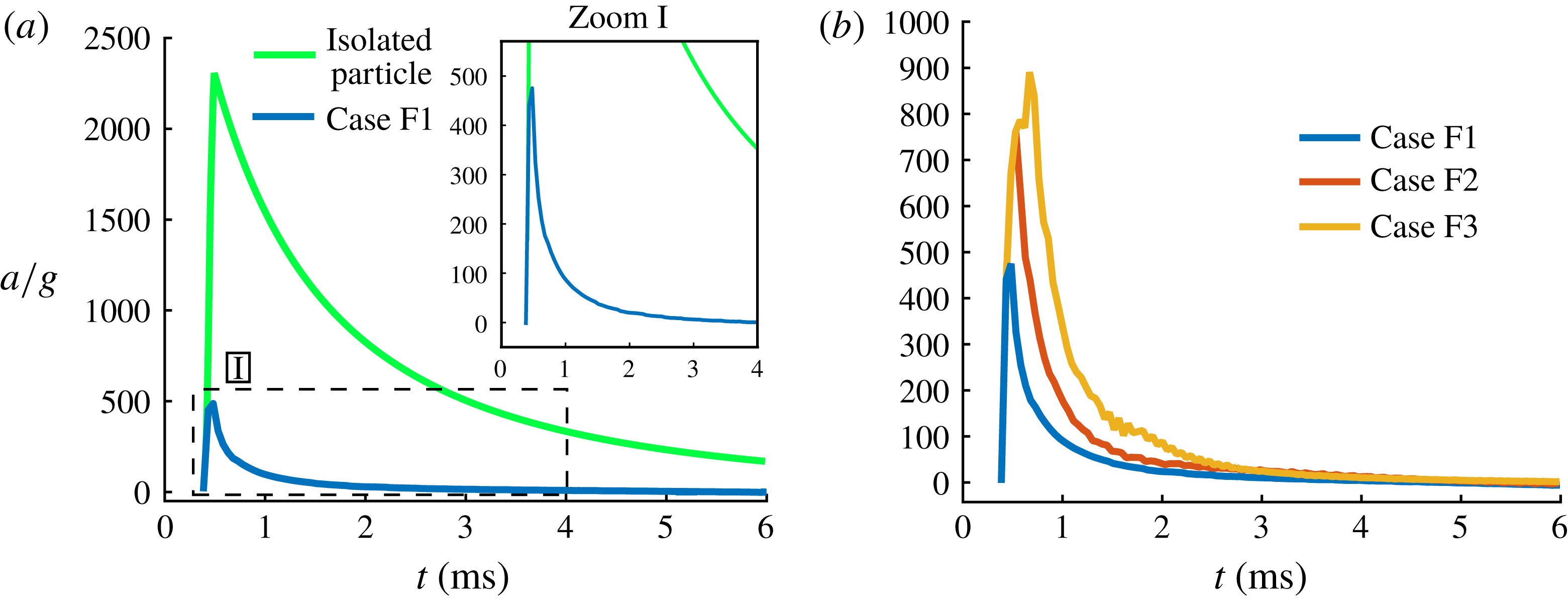
values in the drag model and the shape of the resulting curves exhibited similar characteristics.) The acceleration of the isolated particle was numerically evaluated through integration of the system (3.5) and (3.6). The instantaneous acceleration of this particle is shown in figure 7(a). Additionally, the instantaneous front acceleration is also extracted from the simulation results in case F1 by taking the mean acceleration of particles in the
 $x$
–
 $z$
plane of the uppermost element in which
 $\unicode[STIX]{x1D719}_{p}>0$
. This acceleration is also shown in figure 7(a) for comparison.
Particle front accelerations in time. (a) Case F1 is compared against an isolated particle case and (b) cases F1, F2 and F3.

In figure 7(a), it is clear that the isolated particle overpredicts the acceleration of the front. This is expected since this simple model does not account for the two-way coupling effects of reflection and transmission of the incident rarefaction wave at the front surface, which will weaken the ambient flow as compared to the one-way coupled case. In the zoomed portion of the figure, it is observed that initially the simulated front accelerates much faster than the average value of approximately
 $75g$
, but exponentially decays over a short period. It is interesting to note that the impulse delivered to the particle front, which is proportional to the area under the acceleration curves, is nearly the same between the average
 $75g$
acceleration over 2.5 ms and the time-dependent acceleration from the simulation results. The instantaneous acceleration is much larger than the mean acceleration, with peak accelerations in the simulation reaching nearly
 $475g$
in case F1 and even higher in cases F2 and F3.
In the experiments it was possible to only measure the average acceleration over a sufficiently long time window of 2.5 ms due to the experimental frame rate of 2000 frames per second. As a result, the very strong acceleration at early time was not directly observable in the experiments and therefore was not reported. It appears in figure 7(a) that the simulation results nearly coincide with that of the isolated particle model, during the very early period, when acceleration undergoes a near sudden increase. This very early period is when the head of the expansion fan encounters the top of the initially static particle bed. It can be gathered that during this period the rarefaction wave is not considerably altered by the particle front in case F1. However, when similar results are generated for the cases F2 and F3, the very early time particle front acceleration did not agree with that of the simple isolated particle model nearly as well. Nevertheless, in all cases we observe that the particle front experiences a sudden impulse that can be observed as the rapid rise in the acceleration. The normalized acceleration reaches a peak in a fraction of a millisecond due to the rapid impulsive increase. The acceleration of the particle front remains positive for several milliseconds, but during this period the acceleration magnitude decays exponentially from its peak value.
In figure 7(b) the accelerations from the cases F1, F2 and F3 are given. In all cases it was noted that the simulation impulses well match the experimental impulses obtained from their reported average accelerations. With increasing pressure ratio, the peak acceleration tends to increase and occur somewhat later in time. In essence, even within regime 6, where the particle front undergoes a positive acceleration, two different sub-regimes can be identified based on the rate of change of acceleration: (i) a very short impulsive period when the acceleration reaches a peak and (ii) and a slightly longer period of slow decay of acceleration.
In the work of McGuinness & Singh (Reference McGuinness and Singh2015), a one-dimensional model for the early-time behaviour of the current set-up was developed. The model was able to capture the initial rupture of similar particle beds, which occurred when the gas-induced effective stress in the bed overcame the bed cohesion. The rupture of the bed partitions the initially packed bed into alternating layers of horizontally oriented voids and particle slabs. In the absence of wall friction, it was found that a packed bed of spheres will rupture at a non-dimensional time of
 $\tilde{t}\approx 4\times 10^{-4}$
, corresponding to physical times of
 $t\approx 21,15$
and
 $9.0~\unicode[STIX]{x03BC}\text{s}$
for the present cases F1, F2 and F3. As a result, the peak in acceleration that was observed at early times in figure 7(b) may in part be associated with the initial rupture of the bed. However, while the initial simulation time step of
 $\unicode[STIX]{x0394}t\approx 50$
ns was small enough to resolve these time scales, the solution dump frequency in the simulations was not since output files were only generated every
 $50~\unicode[STIX]{x03BC}\text{s}$
. Thus, we may only speculate that the rupture of the bed plays a role in the initial acceleration of the particle front.
An alternative explanation for the high front acceleration is proposed by considering an individual particle whose acceleration is directly related to the net force acting on it. Thus, we will investigate the two hydrodynamic force components (pressure gradient force
 $\boldsymbol{F}_{un}$
and quasi-steady force
 $\boldsymbol{F}_{qs}$
) that act of the particles during the early period of rarefaction wave interaction with the top of the particle bed. We first note that though pressure is continuous across the head of the rarefaction wave, pressure gradient is discontinuous. Thus, as soon as the rarefaction wave touches the particles, it will instantaneously be subjected to a strong streamwise pressure gradient. The time it takes for an entire particle to be immersed within the non-zero pressure gradient is the particle acoustic time, or the time it takes for the rarefaction head (acoustic wave) to sweep past a particle diameter. In the present case this time scale is very short and can be evaluated to be
 $D_{p}/a_{4}\approx 0.3~\unicode[STIX]{x03BC}\text{s}$
. This is the reason in (3.10) the pressure gradient across the particle was simplified to be a constant. In the simulation however, the discontinuity in pressure gradient is smoothened over several grid spacings, thus contributing to a finite time for the rapid increase in the pressure gradient force. Since the
 $x$
–
 $z$
averaged pressure gradient is nearly a constant across the rarefaction wave, the pressure gradient is the strongest when the rarefaction head first encounters the particle front. At later times, as the rarefaction wave penetrates into the bed, the magnitude of pressure gradient decreases, due to the thickening of the rarefaction wave. This weakening of the pressure gradient force occurs even in the absence of two-way coupling effects.
In contrast to the average pressure gradient, the average gas velocity linearly increases from zero velocity at the rarefaction head to the maximum value of star velocity at the rarefaction tail. Thus, initially the quasi-steady drag is quite small, when only the rarefaction head has penetrated across the top layer of particles. The quasi-steady force, slowly increases as more of the rarefaction wave passes over the particle front. The gas velocity at the particle front will reach its peak value at the instant C when the rarefaction tail reaches the front. In a one-way coupled case, without a reflection at the bottom wall, the gas velocity seen by the advancing particle front will remain the same in the star region. This however is not the case in the present simulations due to both the back effect of particles on the rarefaction wave and due to reflection off the bottom wall. As can be seen in figure 6(c), the gas velocity at the particle front starts to decrease after it initially increases over a fraction of a millisecond.
As the particles start to accelerate upward, they begin to acquire a velocity comparable to the local streamwise gas velocity. For this reason, the relative velocity between the gas and the particles decreases over time, contributing to the post-peak rapid decrease in particle front acceleration. Based on the expression for the quasi-steady force, the particle time scale can be evaluated as
 $$\begin{eqnarray}\unicode[STIX]{x1D70F}_{p}={\displaystyle \frac{\unicode[STIX]{x1D70C}_{p}}{\unicode[STIX]{x1D6FD}}}.\end{eqnarray}$$
Using the largest possible value for
 $\unicode[STIX]{x1D6FD}$
, corresponding to the early time of peak acceleration, we estimate a particle time scale of
 $\unicode[STIX]{x1D70F}_{p}\approx 4$
ms. (Here,
 $\unicode[STIX]{x1D6FD}$
has been estimated for an initially packed bed with
 $|\boldsymbol{U}-\boldsymbol{V}|\approx 10~\text{m}~\text{s}^{-1}$
and
 $\unicode[STIX]{x1D70C}_{f}\approx \unicode[STIX]{x1D70C}_{4}$
.) At later times, when
 $\unicode[STIX]{x1D6FD}$
decreases the particle time scale will increase even more. Thus, we see that the particle time scale is much longer than the decay time scale seen in the acceleration plots of figure 7. As a result, the decay is primarily associated with the rapid reduction in both the gas pressure gradient and the gas velocity at the particle front.
4.4 Back effect of particle front on gas
The previous description has been for the particle front which forms the lower bound of regime 6 in figure 4. Regime 6 is also bounded by the original rarefaction tail and the reflection of the incident rarefaction head. The coordinates of point D can be estimated by assuming the particle front to behave as a solid wall in that the incident rarefaction wave is entirely reflected off it. This is a reasonable assumption since the particle bed rises at a much slower rate than the local sound speed. Under this assumption, it is known from the theoretical work of Tasissa et al. (Reference Tasissa, Hautefeuille, Fitek and Radovitzky2016) that the exit time of the reflected rarefaction head is
 $$\begin{eqnarray}t_{D}=t_{B}\left(\frac{p_{4}}{p_{3}}\right)^{3(\unicode[STIX]{x1D6FE}-1)/2\unicode[STIX]{x1D6FE}},\end{eqnarray}$$
which occurs at the location
 $y_{D}=L_{y}+(u_{3}-a_{3})t_{D}$
where the subscripts correspond to the regimes in figure 4. Note that
 $u_{3}-a_{3}$
is the initial velocity at which the incident rarefaction tail travels. For lower pressure ratios across the diaphragm,
 $a_{3}>u_{3}$
indicating the tail travels down the tube. However, increasing the pressure past a certain critical point will make
 $u_{3}>a_{3}$
so that the incident tail will travel up the tube and the position
 $y_{D}$
will be located above the diaphragm. In the simulations considered, both the incident rarefaction head and tail travel down the tube. For cases F1, F2 and F3, the time
 $t_{D}$
can be estimated as
 $t_{D}\approx 0.42$
, 0.46, 0.51 ms, respectively, which appears to correspond to the slight shift in peaks of the initial front accelerations in figure 7(b).
To estimate the location C we make the approximation that the location of the particle front has not changed much during the early period (
 $\,y_{C}\approx H_{0}$
). The speed of the rarefaction tail is a constant equal to
 $a_{3}-u_{3}$
until it encounters the reflected head at
 $t_{D}$
. After the encounter the speed of the tail continues to increase and increases toward
 $a_{3}$
(Ling et al.
Reference Ling, Wagner, Beresh, Kearney and Balachandar2012). With this observation we can bound the time of interaction between the rarefaction tail and the particle front to be
 $$\begin{eqnarray}t_{D}+{\displaystyle \frac{y_{D}-H_{0}}{a_{3}}}\leqslant t_{C}\leqslant t_{D}+{\displaystyle \frac{y_{D}-H_{0}}{a_{3}-u_{3}}},\end{eqnarray}$$
where the lower limit applies if the tail has increased to the local acoustic speed and the upper limit applies if the tail continued at its original speed. Irrespective, we expect
 $t_{B}<t_{D}<t_{C}$
. During the particle front’s acceleration, the interior shaded region marked as regime 6 in figure 13 sees a spatially and temporally non-uniform gas flow that is imposed on top of the particle front and contributes to the non-zero acceleration of the particle front.
Two mechanisms by which particles alter the flow near the particle front are: (i) reflection and diffraction of the incident wave and (ii) flow channelling. The first mechanism is due to obstruction and is a result of the gas not being able to penetrate the particles. As an extreme example, consider the particle front to be a solid, immovable wall. As the incident rarefaction wave impacts the wall, the gas at the surface of the wall has zero velocity since the wall prevents the flow from penetrating it. In the present case though, the flow is not entirely blocked at the particle front since there are porous void regions between the particles. From this, we can surmise that while the gas velocity at the particle front is not fully zero as it would be if the particles were an impenetrable wall, the gas velocity is substantially slowed at the particle front when compared to a standard single-phase shock tube. The second mechanism that alters the gas flow near the particle front is channelling. Channelling works to locally accelerate the gas through regions of constricted area. The random arrangement of particles leads to nearby regions of locally higher and lower particle volume fractions inside the particle bed. These regions are channels of relatively low particle volume fraction where the gas is able to move more freely than in the neighbouring high volume fraction regions. Due to this, there will be local fluctuations in the gas velocity within the particle bed.
In regime 11, both wave reflection and flow channelling effects are at work near the particle front. These competing effects are seen in case F1 through horizontal
 $x$
–
 $z$
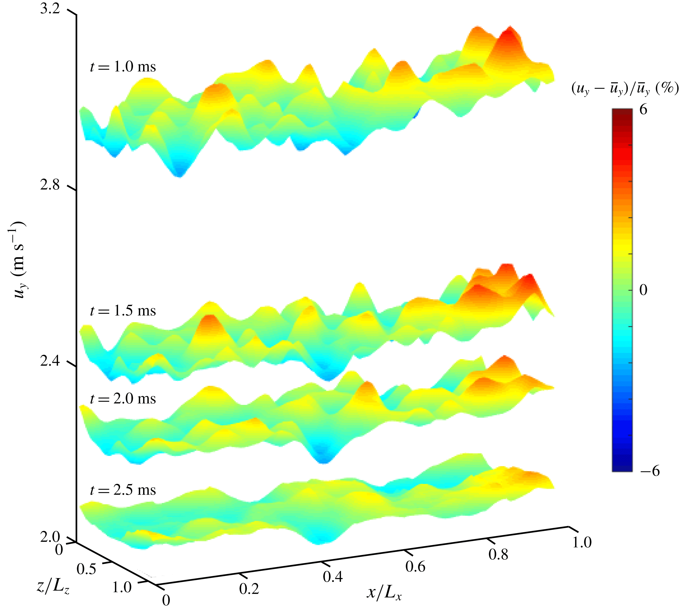
slices of the streamwise fluid velocity at the particle front in figure 8. In this figure, four contours are shown at times of 1, 1.5, 2 and 2.5 ms. These time instants are well past
 $t_{C}$
. The contours are coloured to accentuate the fluctuations from the instantaneous mean flow. The fluctuation intensities are computed by taking the velocity fluctuations
 $u_{y}-\bar{u}_{y}$
and scaling them by the mean instantaneous velocity at the front surface
 $\bar{u}_{y}$
. It is clear that as time progresses, the mean velocity decreases at the particle front as successive contours are shifted down along the vertical axis. This decease in mean streamwise fluid velocity is owed to the obstruction of particles to the gas flow. Simultaneously, as the pressure equilibrates near the particle front, a vertical pressure gradient forms which forces gas through the porous particle bed. In low particle volume fraction channels, the gas is locally accelerated which results in fluctuations of the gas velocity at the particle front. The fluctuations are as much as 6 % of the mean at 1 ms but decrease rapidly thereafter.
Early streamwise fluid velocity at the particle bed front for different times in case F1. The colours are shown as a per cent fluctuation from the mean to accentuate the fluctuations while the vertical axis shows the total velocity.

4.5 Post acceleration evolution of particle front
After the front has finished its initial acceleration, the front enters what we call the constant rise regime. This can be seen in figure 4 from points C and H. Directly above the particle front surface at this stage is regime 12 while below the front surface is regime 11. The properties in regime 12 are of practical importance since they are used to estimate the speeds at which material is ejected in volcanic eruptions (Turcotte et al. Reference Turcotte, Ockendon, Ockendon and Cowley1990; Woods Reference Woods1995; Cagnoli et al. Reference Cagnoli, Barmin, Melnik and Sparks2002; Alatorre-Ibargüengoitia et al. Reference Alatorre-Ibargüengoitia, Scheu, Dingwell, Delgado-Granados and Taddeucci2010).
Due to this, there have been multiple efforts to estimate the post acceleration flow properties at the particle front. In Turcotte et al. (Reference Turcotte, Ockendon, Ockendon and Cowley1990), a relationship between the velocity and pressure of an isothermally expanding pseudo-gas was derived. A pseudo-gas refers to the assumption that the mixture phases are in velocity equilibrium. Following this, Cagnoli et al. (Reference Cagnoli, Barmin, Melnik and Sparks2002) used traditional one-dimensional isentropic theory to provide another relationship between the gas pressure and velocity directly above the particle front by assuming that the incident rarefaction wave fully reflects off the bed. These two pressure–velocity relationships are then solved to obtain a theoretical estimate for the pressure and velocity at the particle front.
Due to wave reflection at the front, a near constant pressure, and therefore velocity, is obtained. In the simulations, we also expect a constant velocity since it was shown in figure 7(b) that the acceleration of the particle front decays to zero after a few milliseconds. We now extract the front velocity from the simulations. This is obtained by tracking the mean position of the particle front in time. Linear regression is then used during the time interval from 2.5 to 6.0 ms to obtain the slope of this curve, which is taken as the front rise velocity. The simulation front velocities are plotted in figure 9, along with the front velocities of the experimental set Q and accompanying one-dimensional theory (Cagnoli et al. Reference Cagnoli, Barmin, Melnik and Sparks2002). It is observed that while there are slight differences, the simulations are in general agreement with the theory and experiments for all the pressure drops considered.
Particle front simulation rise velocities compared to theory and companion experiments of Cagnoli et al. (Reference Cagnoli, Barmin, Melnik and Sparks2002).

4.6 Visualization of bed interior
In figure 4, the interior of the expanding particle bed is characterized by regimes 8, 9, 10, 11 and 13. These regimes include the transmission of the incident rarefaction wave into the particle bed and their subsequent reflection from the bottom wall. In these regimes, the particle bed expands and voids form within the interior of the bed. This expansion can be seen at different times in the volume fraction fields in figure 10.
Volume rendering of particle volume fraction at different times. (a) Case F1, (b) case F2 and (c) case F3.

In figure 10, volume renderings of the particle volume fraction fields every 5 ms are shown for the present simulations. Increasing the initial pressure drop across the diaphragm is associated with a higher rate of expansion of the particle bed. While the structural details of the particle bed are time and space dependent and vary between each case, the overall void evolution can be partitioned into similar stages during each expansion. The stages we observe are: (i) crack formation, (ii) transition of cracks to bubbles and (iii) vertical stretching of the bubbles. While these stages are visible in each of the three simulations, we will use case F1 as a guide to describe the stages.
The formation of cracks is distinguished by the nucleation of horizontally oriented void structures within the bed. The cracks start forming near the top of the bed, as shown at 5 ms in case F1. Even at this time incipient cracks can be discerned throughout the bed, although the strongest ones appear at the front. As time progresses, cracks also begin to strengthen at lower sections of the bed as seen between times of 10 and 20 ms. However, cracks do not appear in the lowest
 ${\approx}1$
cm of the bed near the wall. The original cracks in the upper portion of the bed continue to expand and eventually transition to bubbles, which are more spherical in shape. This is observed around 15–20 ms. Finally, the bubbles near the top of the bed are vertically stretched. An example of this stretching is visible in time from 15–25 ms for the bubble located at approximately
 $y=12$
cm. As time progresses, this bubble elongates from approximately 0.5 cm to nearly 2 cm in the
 $y$
direction.
While the initial conditions of the present simulations are meant to mimic the experiments of Cagnoli et al. (Reference Cagnoli, Barmin, Melnik and Sparks2002), the high speed imaging of the experiments of Anilkumar (Reference Anilkumar1989) and Anilkumar et al. (Reference Anilkumar, Sparks and Sturtevant1993) can be qualitatively compared to the present particle volume fraction renderings. In particular, figure 2 of Anilkumar et al. (Reference Anilkumar, Sparks and Sturtevant1993), which was also reproduced in figure 1 of McGuinness & Singh (Reference McGuinness and Singh2015), is remarkably similar to figure 10 in this work. Most notably, figure 2 of Anilkumar et al. (Reference Anilkumar, Sparks and Sturtevant1993) depicts a similar transition of cracks to bubbles at early times near the top of the bed while cracks at the bottom of the bed appear to remain as cracks.
4.6.1 Void characterization
As the particle bed expands in time, the bed is lengthened due to the rapid depressurization. Due to the expansion, particles are dispersed in a region of fluid that spans a greater volume than the initial packed bed state. Since the number of particles remains constant, there will be a decrease in the average particle volume fraction within the particle–fluid mixture. Due to instabilities this dilution of volume fraction does not occur in a homogeneous manner. We observe the formation of high concentration gas pockets, which are called voids. These voids can be described as either cracks or bubbles. Cracks occur when the horizontal extent of a void is much larger than its vertical extent. Alternatively, bubbles are voids that extend nearly the same distance in all three directions. Here, we characterize the voids based on three main properties: (i) void size, (ii) void position and (iii) void shape.
While it may be difficult to visualize and quantify voids in experiments, this can be done with relative ease in the simulations. Numerically, voids can be identified from the volume fraction field
 $\unicode[STIX]{x1D719}_{p}(\boldsymbol{x})$
by creating closed isosurfaces where the volume fraction on each isosurface is specified as
 $\unicode[STIX]{x1D719}_{p,v}$
. The void region is then the volume inside each closed isosurface whose particle volume fraction within it is less than or equal to
 $\unicode[STIX]{x1D719}_{p,v}$
. Note that the cut-off volume fraction
 $\unicode[STIX]{x1D719}_{p,v}$
must be chosen carefully since the void intensity will directly depend on the problem set-up. The number of closed isosurfaces at a given volume fraction threshold will be called the number of voids and denoted by
 ${\mathcal{N}}_{{\mathcal{V}}}$
.
At a given time for a given volume fraction threshold, the size of each individual void can be characterized by its volume. In particular, a non-dimensional void size
 ${\mathcal{V}}_{{\mathcal{V}}}$
is computed as the volume inside a given closed isosurface
 $V_{v}$
divided by the particle volume
 $V_{p}$
. In this way,
 ${\mathcal{V}}_{{\mathcal{V}}}$
is a measure of how much larger a void is compared to the particle’s volume. The position of each void can be characterized by its volumetric centroid. The vertical coordinate of the centroid, given by
 $Y_{c}$
, is then non-dimensionalized by the initial height of the particle bed
 $H_{0}$
to obtain the non-dimensional void position
 ${\mathcal{Y}}_{{\mathcal{V}}}$
. Values of
 ${\mathcal{Y}}_{{\mathcal{V}}}$
less than one correspond to voids within the original unexpanded bed, while values greater than one are voids occurring above the original bed. Finally, the shape of each void is quantified by the extent of each isosurface in the horizontal and vertical directions. The minimum point on each surface in each direction is subtracted from the maximum point on the surface in the corresponding direction to form the directional void lengths
 $l_{v,x}$
,
 $l_{v,y}$
and
 $l_{v,z}$
. The ratio of this length in the vertical to the horizontal directions then provides an estimate of a void’s shape. This ratio will characterize the void shape and will be called the void aspect ratio
 ${\mathcal{A}}_{{\mathcal{V}}}$
. The void aspect ratio will typically range from nearly zero to around one. Aspect ratios close to one corresponds to bubbles while values much less than one correspond to cracks. These three void properties are computed by
 $$\begin{eqnarray}{\mathcal{V}}_{{\mathcal{V}}}=\frac{V_{v}}{V_{p}},\quad {\mathcal{Y}}_{{\mathcal{V}}}=\frac{Y_{c}}{H_{0}},\quad {\mathcal{A}}_{{\mathcal{V}}}=\frac{l_{v,y}}{\max (l_{v,x},l_{v,z})}.\end{eqnarray}$$
Following this, each void has a set of properties associated with it, which include its volume, position, and aspect ratio. If we examine a single simulation at a particular instance in time, an empirical cumulative distribution function (ECDF) can be built for each property. Here, we define the void ECDF in each case as
 $$\begin{eqnarray}F_{{\mathcal{N}}_{{\mathcal{V}}}}^{\unicode[STIX]{x1D719}_{p,v}}(x)=\frac{1}{{\mathcal{N}}_{{\mathcal{V}}}}\mathop{\sum }_{i=1}^{{\mathcal{N}}_{{\mathcal{V}}}}I(x_{i}\leqslant x),\end{eqnarray}$$
where
 $x$
may be any of the three void properties previous listed and
 $I(x_{i}\leqslant x)$
is the indicator function for property
 $x$
. The indicator function is zero unless
 $x_{i}\leqslant x$
, otherwise it is one. Due to the scaling by the number of voids, it is seen then that
 $F_{{\mathcal{N}}_{{\mathcal{V}}}}^{\unicode[STIX]{x1D719}_{p,v}}(x)$
ranges from zero to one and indicates the cumulative probability of a void property taking a value less than
 $x$
.
4.6.2 Void dynamics
When the incident rarefaction head initially impacts the particle bed, it propagates at the speed of sound in the particle bed. Since the particles are much heavier than the gas, the bed is initially at rest as the flow travels inside the bed. Under these conditions, the frozen speed of sound within the bed can be approximated (Rudinger Reference Rudinger1980) as
 $$\begin{eqnarray}a_{E}=\frac{a_{4}}{\sqrt{\unicode[STIX]{x1D719}_{f}}}.\end{eqnarray}$$
If we assume a random close packing of
 $\unicode[STIX]{x1D719}_{p}\approx 0.64$
and a driver gas sound speed of
 $a_{4}=343~\text{m}~\text{s}^{-1}$
, the frozen sound speed is
 $a_{E}=572~\text{m}~\text{s}^{-1}$
. The time
 $t_{E}$
(refer to figure 4) when the transmitted head reaches the bottom wall is then
 $t_{E}\approx t_{B}+H_{0}/a_{E}=0.56$
ms. Thus, after a very short time, void formation can initiate within the entire bed. Despite the rapid transmission of the rarefaction wave into the bed, the formation of voids will be delayed, since particles require a finite time in order to respond to the increased gas flow around them.
For case F1, the empirical cumulative distribution function of void position, volume and aspect ratio are shown in figure 11 at various stages in the bed’s expansion. In the figure, we have used
 $\unicode[STIX]{x1D719}_{p,v}=30\,\%$
as the cutoff volume fraction. In figure 11(a), the void position is shown. At 5 ms, nearly all of the voids are located near the top of the bed. By 10 ms, these voids have travelled up with the particle front while new ones have opened deeper within the bed. Additionally, at this time there is a near uniform distribution of voids throughout the upper half of the bed, as shown by the near linear cumulative distribution. From 10–15 ms, the position of voids transitions from this uniform distribution to what appears to be two distinctive uniform distributions that are separated at
 ${\mathcal{Y}}_{{\mathcal{V}}}\approx 0.4$
. Reading directly from the plot then, we can see that approximately 50 % of the voids are found between
 ${\mathcal{Y}}_{{\mathcal{V}}}\in [0.2,0.4]$
while the remaining half are found in
 ${\mathcal{Y}}_{{\mathcal{V}}}\in [0.4,1.1]$
. In
 ${\mathcal{Y}}_{{\mathcal{V}}}\in [0.0,0.2]$
, there are no discernible voids. Thus, there is a higher density of voids in the bottom portion of the bed than in the upper portion of the bed at 15 ms. This is indicative of the fact that the voids are smaller in size in the bottom portion of the bed as compared to the top. The voids at later times remain similarly distributed.
Regarding the void volumes, figure 11(b) shows that initially at 5 ms the voids are relatively small with the maximum volume of a void being
 ${\mathcal{V}}_{{\mathcal{V}}}\approx 2000$
. As time progresses, the voids grow in size, resulting in the largest void at 25 ms being of size
 ${\mathcal{V}}_{{\mathcal{V}}}\approx 10^{5}$
. Even still, at this stage the larger voids are uncommon since approximately 70 % of the voids are over 10 times smaller than the largest void. Regarding the void aspect ratio in figure 11(c), an increase from low to moderate aspect ratios is observed as time progresses. Nearly all of the voids at 5 ms have
 ${\mathcal{A}}_{{\mathcal{V}}}<0.5$
, meaning that they appear as cracks rather than bubbles. At later times, the aspect ratios increase as the cracks transition to bubbles.
Particle void ECDF at different times in case F1 for cutoff volume fraction
 $\unicode[STIX]{x1D719}_{p,v}=30\,\%$
. (a) Void position, (b) void volume and (c) void aspect ratio.

4.6.3 Correlation of void properties
We now consider joint probability distributions of void properties. A two-variable empirical cumulative density function is computed by
 $$\begin{eqnarray}F_{{\mathcal{N}}_{{\mathcal{V}}}}^{\unicode[STIX]{x1D719}_{p,v}}(x,y)=\frac{1}{{\mathcal{N}}_{{\mathcal{V}}}}\mathop{\sum }_{i=1}^{{\mathcal{N}}_{{\mathcal{V}}}}I(x_{i}\leqslant x,y_{i}\leqslant y),\end{eqnarray}$$
where
 $x$
and
 $y$
are the two void properties that we seek to correlate. The joint probability function
 $f_{{\mathcal{N}}_{{\mathcal{V}}}}^{\unicode[STIX]{x1D719}_{p,v}}$
can then be computed by taking the directional derivatives with respect to each property as
 $$\begin{eqnarray}f_{{\mathcal{N}}_{{\mathcal{V}}}}^{\unicode[STIX]{x1D719}_{p,v}}(x,y)=\frac{\unicode[STIX]{x2202}^{2}F_{{\mathcal{N}}_{{\mathcal{V}}}}^{\unicode[STIX]{x1D719}_{p,v}}}{\unicode[STIX]{x2202}x\unicode[STIX]{x2202}y}.\end{eqnarray}$$
This process can be extended to obtain a joint probability density function correlating all three void properties. However, we have limited the present work to correlations between only two void properties.
The joint probability density functions for void position and void aspect ratio in case F1 are shown in figure 12. In the figure, the void position is on the vertical axis while the void aspect ratio is on the horizontal axis. The time increases from 5 ms in frame A to 25 ms in frame E. The red regions are associated with high probabilities, while the blue regions correspond to low probabilities. From this figure, we can see that the initial voids appear near the top of the bed as cracks, which is indicated by the smaller aspect ratio. As time progresses, cracks also begin to form at lower portions of the bed. While the voids at the lower portion of the bed appear to remain as cracks, the cracks near the top of the bed increase in their aspect ratio as they transition to bubbles.
While not shown here, we have also looked at the joint probability distribution of void position paired with void volume and the joint probability distribution of void volume paired with void aspect ratio. These joint distributions also show a positive correlation between void volume and void position and a positive correlation between void volume, void position and void aspect ratio. From these results, it can be surmised that cracks that appear near the top of the bed will turn into bubbles as time goes on. During this transition at the top of the bed, the lower portions of the bed will also start to form cracks. In contrast to the cracks at the top of the bed, the cracks in the lower portion of the bed tend to stay as cracks.
Additionally, we see that bubbles are associated with the larger volumes, which has practical consequences. The outflow of particle–gas mixture at the upper portions of the domain will be highly inhomogeneous. The inhomogeneity is characterized by bubble-like pockets of gas dispersed throughout regions of gas–particle mixture. In these regions of gas–particle mixture, we see higher than average concentrations of particles, with local particle volume fractions that are just as large as their initially packed state.
Joint probability distributions of the void aspect ratio (horizontal axis) and the void position (vertical axis) for case F1. The panels are presented every 5 ms and are ordered in increasing time; (a) 5.0 ms, (b) 10.0 ms, (c) 15.0 ms, (d) 20.0 ms and (d) 25.0 ms.

4.6.4 Mechanism of void growth
In the experiments of Cagnoli et al. (Reference Cagnoli, Barmin, Melnik and Sparks2002), another interesting feature that was observed was the vertical slow down and reversal of voids within the bed for lower pressure drops in the range of 20–40 kPa. We see a similar behaviour in simulation F1, which falls within this range since
 $\unicode[STIX]{x0394}p=30$
kPa. For example, in figure 13, the slow down and reversal of a void is shown in the upper portion of the bed through a zoomed view of the particle volume fraction contours. The void can hardly be seen initially but becomes clear as time goes on. As the void opens, it initially travels upwards from 7.5–15.0 ms. Then, from 15.0–22.5 ms the void travels back downwards. On its descent, it is observed that it is much more devoid of particles than it was initially.
Zoomed view of case F1 particle volume fraction. The window is of
 $x\in [0.48,0.95]$
cm and
 $y\in [8.33,9.07]$
cm. The slow down and reversal of a single void is shown in the dashed box.

In addition to Cagnoli et al. (Reference Cagnoli, Barmin, Melnik and Sparks2002), similar experiments were earlier performed by Anilkumar (Reference Anilkumar1989) in order to study the growth of voids within the bed. This work observed the voids to start as cracks and transition to bubbles. It was noted that the growth of bubbles was due to the column-like dripping of particles from the top of a void to the bottom of the void. Due to the high mass loading of particles, it was suggested that the mechanism was, ‘analogous to the Rayleigh–Taylor instability observed in continuous media’ (Anilkumar Reference Anilkumar1989). Rayleigh–Taylor instabilities occur when a fluid of high density is stacked on top of a fluid of low density. When perturbed, the lighter fluid will rise and partition the stratified mixture into column-like vertical structures of alternating fluids. The simulation results do not fully support this viewpoint since particles do not necessarily behave as a continuous media, and an alternative mechanism is advanced.
Initially, the particles in the present multiphase shock tube appear to be fluidized. While not always the case, fluidized particles will often behave as a continuum. (A notable exception of this is given by Fortes, Joseph & Lundgren (Reference Fortes, Joseph and Lundgren1987) where it was found that the relative locations of nearby particle–wake interactions dominated the fluidized system dynamics.) Despite the similarity to fluidization, there are also important differences. In fact, Cagnoli et al. (Reference Cagnoli, Barmin, Melnik and Sparks2002) pointed out some of the key differences between traditional fluidization and the rapid depressurization of particles. Most important among these differences is in the generation of bed expansion. In fluidization, expansion occurs by an injection of gas through the bottom of a particle bed, while in the shock tube the bed expansion starts from the top and moves down due to the transmission of the incident rarefaction wave. Perhaps, due to these differences, the growth of voids is not necessarily a result of a multiphase Rayleigh–Taylor-type instability.
We offer an alternative mechanism for void growth that is based solely on direct observations from the present simulations. In order to motivate our explanation, we have presented a schematic of two possible void growth mechanisms in figure 14. In frame A, a single void is shown at early times with a small aspect ratio. Note that the centroid is shown inside the void, which corresponds to the void’s volume fraction weighted mean vertical position. The shaded regions in and around the void denote high and low particle volume fractions. By definition, the volume fraction outside the void is
 $\unicode[STIX]{x1D719}_{p}>\unicode[STIX]{x1D719}_{p,v}$
while inside it is
 $\unicode[STIX]{x1D719}_{p}\leqslant \unicode[STIX]{x1D719}_{p,v}$
. As time progresses, the model void both grows and travels in the vertical direction as shown in frame B. At this later time, the volume fraction inside the void is still less than the threshold
 $\unicode[STIX]{x1D719}_{p,v}$
. While the growth is associated with an increase in void volume, its motion is indicated by the movement of the centroid. To explore the mechanistic roots of this simultaneous growth and motion of the void, we must allow for both entrainment of particles into the void from surrounding higher volume fraction regions and detrainment of particles from the void to the surroundings. The asymmetry in the manner which this entrainment and detrainment process occurs at the periphery of the void will determine the different mechanisms and the mode of void growth.
Possible void growth mechanisms. (a) The original void is shown, (b) the void is vertically stretched as time progresses and (c) different particle concentrations are shown inside the stretched void and are indicative of different growth mechanisms.

Since the entire region occupied by the void at later times (frame B) is above the upper surface of its initial configuration, the void has clearly travelled upwards (also indicated by the centroid). For the moment consider a frame of reference travelling at the mean upward velocity of the void, so attention can focus only on the void growth process. In frame C, two possible mechanisms are used to explain the void growth. The first will be called the dripping mechanism, which is the previously mentioned Rayleigh–Taylor type growth. The second is the lifting mechanism and is shown on the right of frame C. The differences between the mechanisms are found in where particles are entrained and detrained at the void surface. In this case, we define entrainment to be the process of particles originally outside of voids entering into the voids. Conversely, detrainment is defined as the process of particles originally inside voids exiting to the surroundings. From the present simulations, we have observed a gradual change in volume fraction at the void surface to be associated with entrainment while a sharp change in volume fraction is associated with detrainment.
In the dripping mechanism, the particles entrain into the void from the top while they are detrained at the bottom of the void. The volume fraction variation is gentle at the top of the void where the particles entrain into the void by dripping (although, by definition, the upper boundary of the void is denoted by a sharp interface of
 $\unicode[STIX]{x1D719}_{p}=\unicode[STIX]{x1D719}_{p,v}$
). As particles rain down to the bottom surface of the void, their path is blocked from below by the high particle concentration outside the void. Thus, the particle volume fraction variation at the detraining front at the bottom is expected to be much sharper. In the figure this blockage is shown by the discontinuity in volume fraction at the bottom of the void. Furthermore, as the particles pile up at the bottom of the void, there will be increased collisions. Since the concentration of particles inside the void is higher near the top, the particle volume fraction weighted centroid is shown skewed towards the upper half of the void when compared to the void’s geometric centre.
Alternatively, the void can be enlarged by the lifting mechanism which is shown in the right of frame C. In this mechanism, the particles entrain into the void from the bottom while they are detrained at the top. The volume fraction variation is gentle at the bottom where the particles are lifted. As particles pile up at the top, the particle volume fraction variation there will be sharp. As a result, we can expect increased collisions and higher inter-particle collisional forces at the top. In this mechanism, the centroid will be skewed towards the bottom half of the void.
We now use the simulation results to explore the possibility of these different void growth mechanisms. This will be accomplished by focusing on the following three void growth characteristics: (i) the relative location of a void’s particle volume fraction weighted centroid to its geometric centre, (ii) the sharpness of volume fraction variation near a void’s surface and (iii) the number and intensity of collisions at the top and the bottom of the void region. Thus, monitoring these features from our simulations will give us confidence in determining the mechanism by which we observe void growth.
Zoomed view of the time evolution of particles in case F2. The region is bounded by
 $y\in [12,13]$
cm and spans the entire domain width in
 $x$
. When present, the axes tick marks occur every 0.25 cm. (a) Contours of particle volume fraction field, (b) closed volume fraction isosurfaces showing the voids with
 $\unicode[STIX]{x1D719}_{p,v}=15\,\%$
, (c) volume fraction contours on a planar slice at
 $z=1.78$
mm and (d) collision force magnitude of individual colliding particles outside the voids.

In order to determine which growth mechanism is dominant, we have looked at a zoomed view of the particle evolution in time for case F2 in figure 15. In the figure, a window of
 $x\in [0,0.95]$
cm and
 $y\in [12,13]$
cm is shown. From the left column to the right column time increases from 13.5 to 15.0 ms at 0.5 ms increments. In row (a), contours of the projected volume fraction field are shown. Then, in row (b) closed isosurfaces of the volume fraction are depicted, which correspond to voids with
 $\unicode[STIX]{x1D719}_{p,v}=15\,\%$
. In the dashed portion of this frame, the vertical growth of a single void in the interior of the bed is observed. In row (c), a slice midway through the domain with
 $z$
normal direction is taken at
 $z=1.78$
mm. Here, the particle volume fraction is still plotted but the bounds have been changed to accentuate the lower volume fractions seen inside the voids. The dashed region at each time in row (c) is the planar slice of the void circled in row (b). It is observed that within the void, the change in volume fraction at the bottom surface is more gradual than at the top. In the figure, this is illustrated by the thickness of the transition between red (
 $\unicode[STIX]{x1D719}_{p}=15\,\%$
) and green (
 $\unicode[STIX]{x1D719}_{p}=7.5\,\%$
) from 13.5 to 15.0 ms on the top and bottom surfaces of the void. Additionally, we computed the volume fraction weighted centroid to be approximately 1 % lower than the geometric centre when compared to the void’s vertical extent
 $l_{v,y}$
. This trend of a gradual change on the bottom surface and a sharp change on top surface persists at every time shown here, suggesting that the lifting mechanism is dominant.
In row (d), individual particles in collision outside of voids are shown coloured by their collision force magnitude. Thus, the empty spaces devoid of particles represent the void regions. It is seen that collision force bands appear with horizontal striations of alternating high and low magnitude collision forces. The high collision force bands are located directly above each void while the low collision forces occur near the bottom surfaces of voids. This is interpreted as more collisions taking place at the top surfaces of voids because the detraining particles are blocked by the high concentration layer of particles just above each void. Due to this, the collision force bands provide further support for the lifting growth mechanism since the sharp blockage in the voids occur at the top surface. Each of these observations in support of the lifting mechanism were made not only for the void shown in figure 15 but also for many other voids that we similarly tested.
5 Conclusions
Numerical simulations of the rapid depressurization of a packed bed of glass particles in a shock tube were performed using the Euler–Lagrange method. Our results were compared and contrasted with the experimental work of Cagnoli et al. (Reference Cagnoli, Barmin, Melnik and Sparks2002). In order to characterize the simulation results, surface features of the particle front and void dynamics inside the bed were detailed.
Three high-fidelity three-dimensional simulations were considered. Between each simulation, the pressure difference across the shock tube diaphragm was varied resulting in pressure differences of 30, 50 and 70 kPa. From the simulation results, a regime map was constructed which detailed the various wave interactions observed in the simulations. It was shown that the presence of the particles in the shock tube resulted in considerably more complex wave interactions than in a traditional single-phase shock tube. These interactions are understood as transmitted and reflected waves at both the particle front surface and within the interior of the bed.
At the particle front, the fluid pressure and velocity reached a constant state within only a few milliseconds after the diaphragm burst. In this short time, the particles at the front were rapidly accelerated, reaching peak accelerations of nearly 1000 times that of standard gravity. While the impulses delivered to the particle bed were comparable between our work and the experiments of Cagnoli et al. (Reference Cagnoli, Barmin, Melnik and Sparks2002), the simulations showed more highly time-varying accelerations than the experiments. The initial rapid increase in acceleration occurred at the acoustic time scale and was associated with the initial transmission and reflection of the incident rarefaction wave at the particle bed surface. Following this, the particles equilibrated with the surrounding fluid flow and we saw a more gradual decrease in the particle’s acceleration due to viscous drag. After accelerating, the particle–gas mixture at the bed front then travelled at a near constant velocity, with speeds in good agreement with both the experiments and a one-dimensional theoretical model.
In the interior of the bed, the formation and growth of voids was detailed. The voids initially appeared as horizontally oriented cracks in the expanding bed. At the top of the bed, the cracks transitioned to bubbles at later times, and were more isotropic in shape than the cracks. As this transition occurred, the voids also grew in size. During the void growth process, we found evidence for a lifting mechanism of void growth, which was different from a previously suggested dripping mechanism (Anilkumar Reference Anilkumar1989). We found that rather than particles raining down from the top to the bottom layers inside voids, the particles were being lifted from the bottom to the top of each void. The lifting of particles inside voids was unexpected and may help to explain surprising behaviour, such as the slow down and reversal of voids (Cagnoli et al. Reference Cagnoli, Barmin, Melnik and Sparks2002). Future studies, both experimental and numerical, should be performed to see if this mechanism persists at higher pressure ratios and under what conditions the lifting mechanism dominates the dripping mechanism.
Acknowledgements
We would like to thank Dr J. Hackl for his help in extending the conservation equations in the gas solver to include multiphase coupling terms. This material is based upon work supported by the National Science Foundation Graduate Research Fellowship under grant no. DGE-1315138. This work was also supported in part by the US Department of Energy, National Nuclear Security Administration, Advanced Simulation and Computing Program, as a Cooperative Agreement under the Predictive Science Academic Alliance Program, under contract no. DE-NA0002378.