1 Introduction
The mathematical analysis of stochastic point processes has been an object of study for applied probabilities for many years (Cox, Reference Cox1955; Bartlett, Reference Bartlett1963; Snyder, Reference Snyder1975; Cox & Isham, Reference Cox and Isham1980, Reference Cox and Isham1986; Brémaud, Reference Brémaud1981; Daley & Vere-Jones, Reference Daley and Vere-Jones2003, Reference Daley and Vere-Jones2008). In practice, to count number of points in time on which a point process is defined, counting processes such as the Poisson, Cox, Hawkes and dynamic contagion process have been used. They have been used to count the number of claims/losses in insurance modelling and the number of defaults in credit risk modelling.
The Poisson process, named after the French mathematician Siméon-Denis Poisson, is found to be an appropriate model in many applications including experiments on radioactive decay, and telephone call arrivals. It has been used in numerous disciplines such as astronomy, biology, ecology, geology, seismology, physics, economics, image processing and telecommunications (https://en.wikipedia.org/wiki/Poisson_point_process). The Poisson process is the simplest process associated with counting number of points as it has deterministic intensity and memoryless property. However, even though it is the simplest process in the counting process family, the Poisson process is important as it is an essential building block to move up to more complicated counting processes, i.e., the Cox process, the Hawkes process, shot-noise Poisson process and the dynamic contagion process.
The Cox process, named after the British statistician David Cox (Reference Cox1955), is a generalisation of the Poisson process. Under the Cox process, its intensity function is assumed to be stochastic. The Cox process provides flexibility by letting the intensity not only depending on time but also allowing it to be a stochastic process. Hence, in the Cox process, we can consider various stochastic processes for its intensity. The applications of Cox process in insurance context can be found in Grandell (Reference Grandell1991, Reference Grandell1997), Rolski et al. (Reference Rolski, Schmidli, Schmidt and Teugels1998), Basu & Dassios (Reference Basu and Dassios2002), Bening & Korolev (Reference Bening and Korolev2002), Dassios & Jang (Reference Dassios and Jang2003, Reference Dassios and Jang2005, Reference Dassios and Jang2008), Albrecher & Asmussen (Reference Albrecher and Asmussen2006), Dassios et al. (Reference Dassios, Jang and Zhao2015) and Jang et al. (Reference Jang, Park and Jang2018b).
The Hawkes process, named after the British statistician Alan Hawkes (Reference Hawkes1971a, Reference Hawkesb), is an extension of the Poisson process with self-exciting property, where points show clustering effects. Self-exciting (or Hawkes) processes (Hawkes, Reference Hawkes1971a, Reference Hawkesb, Reference Hawkes1972; Hawkes & Oakes, Reference Hawkes and Oakes1974; Daley & Vere-Jones, Reference Daley and Vere-Jones2003) are versatile point processes, interesting from both a theoretical and a practical point of view. The theoretical foundation of Hawkes processes can be traced from a series of paper written by Brémaud & Massoulié (Reference Brémaud and Massoulié1996, Reference Brémaud and Massoulié2001, Reference Brémaud and Massoulié2002) and Liniger (Reference Liniger2009). Relevant publications in seismology and the modelling of the occurrence of earthquakes are Vere-Jones (Reference Vere-Jones1975, Reference Vere-Jones1978), Adamopoulos (Reference Adamopoulos1976), Ozaki (Reference Ozaki1979), Vere-Jones & Ozaki (Reference Vere-Jones and Ozaki1982) and Ogata (Reference Ogata1988).
The applications and modelling of Hawkes processes in finance can be found in Chavez-Demoulin et al. (Reference Chavez-Demoulin, Davison and McNeil2005), McNeil et al. (Reference McNeil, Frey and Embrechts2005), Bowsher (Reference Bowsher2007), Bauwens & Hautsch (Reference Bauwens and Hautsch2009), Bacry et al. (Reference Bacry, Mastromatteo and Muzy2015) and Hawkes (Reference Hawkes2018). Credit default modelling using these processes can be noticed in Errais et al. (Reference Errais, Giesecke and Goldberg2010) and Giesecke & Kim (Reference Giesecke and Kim2011). Stabile & Torrisi (Reference Stabile and Torrisi2010) applied Hawkes process in insurance context studying the asymptotic behaviour of infinite and finite horizon ruin probabilities.
Embrechts et al. (Reference Embrechts, Liniger and Lin2011) showed that multivariate Hawkes processes can be applied to the stock market indices. The applications and modelling of multivariate Hawkes process in high-frequency limit order book data can be found in Rambaldi et al. (Reference Rambaldi, Bacry and Lillo2017) and Lu & Abergel (Reference Lu and Abergel2018). Yang et al. (Reference Yang, Liu, Chen and Hawkes2018) investigated the interactions between market return events and investor sentiment using a multivariate Hawkes process. Gao et al. (Reference Gao, Zhou and Zhu2018) applied the joint Laplace transform of the classical Hawkes process and its compound process in dark pool trading, which do not display bid and ask quotes to the public. Jang & Dassios (Reference Jang and Dassios2013) introduced a bivariate shot-noise self-exciting process that can be used for the modelling of catastrophic losses. Dassios & Zhao (Reference Dassios and Zhao2013) introduced the numerical algorithm of exact simulation for Hawkes process with exponentially decaying intensity extending it to multi-dimensions.
Numerous papers have also looked at the modelling of financial and insurance risks incorporating Hawkes processes into diffusion models. Aït-Sahalia et al. (Reference Aït-Sahalia, Cacho-Diaz and Laeven2015) used a mutually exciting jump-diffusion process to model six stock market indices. Portfolio selections using Hawkes jump-diffusion models can be noticed in Aït-Sahalia & Hurd (Reference Aït-Sahalia and Hurd2016) and Bian et al. (Reference Bian, Chen and Zeng2019). Liu & Zhu (Reference Liu and Zhu2019), Hainaut & Moraux (Reference Hainaut and Moraux2018, Reference Hainaut and Moraux2019) and Ma et al. (Reference Ma, Shrestha and Xu2017, Reference Ma, Pan and Wang2020) contain Hawkes jump-diffusion models in pricing and hedging context. Maneesoonthorn et al. (Reference Maneesoonthorn, Forbes and Martin2017) modelled the price and stochastic volatility of an asset using a joint Hawkes process in conjunction with a bivariate jump diffusion for an empirical investigation on the S $\&$P 500 market index. The applications of Hawkes jump-diffusion models have been reviewed by Hawkes (Reference Hawkes2020). Dassios & Zhao (Reference Dassios and Zhao2017a) developed exact simulation algorithms for a family of generalised self-exciting point processes with Cox-Ingersoll-Ross (CIR) type intensities. Dassios et al. (Reference Dassios, Jang and Zhao2019) studied a generalised CIR process with externally exciting and self-exciting jumps for insurance premium calculations and default-free zero-coupon bond pricing.
Shot noise occurs in connection with electron emissions from the cathode. Walter Schottky (Reference Schottky1918), who studied fluctuations of current in vacuum tubes, introduced the concept of shot noise. Shot-noise Poisson process is another extension of the Poisson process, where it is capable of displaying the frequency, magnitude and time period needed to determine the effect of points. The applications of shot-noise Poisson process in insurance and credit risk context can be noticed in Klüppelberg & Mikosch (Reference Klüppelberg and Mikosch1995), Jang (Reference Jang2004), Jang & Krvavych (Reference Jang and Krvavych2004), Herbertsson et al. (Reference Herbertsson, Jang and Schmidt2011) and Jang et al. (Reference Jang, Dassios and Zhao2018a).
The dynamic contagion process, which is a generalisation of the externally exciting Cox process with shot-noise intensity and the self-exciting Hawkes process, was introduced by Dassios & Zhao (Reference Dassios and Zhao2011) applying to credit risk. Dassios & Zhao (Reference Dassios and Zhao2012) also examined infinite horizon ruin probability with its Monte Carlo simulation using this process as the claim arrival process. Dassios & Zhao (Reference Dassios and Zhao2017b) extended this process with diffusion component, i.e., self-exciting, externally exciting and mean-reverting stochastic intensity to calculate the default probability and to price defaultable zero-coupon bonds.
Multivariate extension on the dynamic contagion process can be noticed in Dong (Reference Dong2014). She introduced the bivariate dynamic contagion process including the cross-exciting contagion effect, providing its exact simulation algorithm. The stationarity and the diffusion approximation of this process have been explored, where obtained Kalman–Bucy filter was used to calculate stop-loss reinsurance premium. She also showed that a sequence of scaled intensity process of the univariate dynamic contagion processes converges to a CIR process weakly in the path space, with which an alternative approximation simulation scheme for CIR process and the Heston model was developed. Jang & Oh (Reference Jang and Oh2020) introduced a bivariate compound dynamic contagion process for the modelling of aggregate losses from cyber events.
To promote the Poisson, Cox, Hawkes, shot-noise Poisson and dynamic contagion process and their compound processes widespread dissemination in academia and industry further, we revisit their distributional properties. What we present in this paper facilitate the usage of them in practice, enabling researchers to understand their probability characteristics. Given the current COVID-19 pandemic, it is envisaged that more multivariate works will be made to deal with the arrival of multiple, catastrophic and contagious losses accommodating the interdependence between risks.
This paper is structured as follows. In section 2, we provide a mathematical definition of the dynamic contagion process. We also provide the infinitesimal generator of the dynamic contagion process, a generalised Hawkes process and the Cox process with shot-noise Poisson intensity, respectively. This section offers the joint Laplace transform – probability generating function, which is adopted from Dassios & Zhao (Reference Dassios and Zhao2011). By setting appropriate values to the relevant parameters, shot-noise self-exciting Poisson process, shot-noise self-exciting process, shot-noise Poisson process, the compound Poisson process and the Poisson process are also discussed. In section 3, we deal with the compound dynamic contagion process, a generalised compound Hawkes process and the compound Cox process with shot-noise Poisson intensity. We analyse the compound dynamic contagion process systematically for its theoretical distributional property, based on the piecewise deterministic Markov process theory developed by Davis (Reference Davis1984), and the martingale methodology used by Dassios & Jang (Reference Dassios and Jang2003). In section 4, we present the moments and simulation algorithms for the compound processes. We also provide numerical comparisons of value-at-risk (VaR) and tail conditional expectation (TCE or TailVaR) as an application of these processes. Section 5 concludes the paper.
2 Dynamic Contagion Process, Hawkes Process and Cox Process
2.1 Definition
In this section, we present the dynamic contagion process, based on which a generalised Hawkes process and the Cox process with shot-noise Poisson intensity are presented as its special cases. These processes are within the general framework of affine processes, for that see Duffie et al. (Reference Duffie, Pan and Singleton2000), Duffie et al. (Reference Duffie, Filipović and Schachermayer2003) and Glasserman & Kim (Reference Glasserman and Kim2010). By setting appropriate values to the relevant parameters, we also deal with shot-noise self-exciting Poisson process, shot-noise self-exciting process, shot-noise Poisson process, the compound Poisson process and the Poisson process.
2.1.1 Dynamic contagion process
Let us start with a mathematical definition for the dynamic contagion process (DCP) in Definition 2.1 via the stochastic intensity representation. For an alternative definition for this process, we refer you Dassios & Zhao (Reference Dassios and Zhao2011), Jang & Dassios (Reference Jang and Dassios2013) and Dong (Reference Dong2014), where they gave a cluster process representation for this process.
Definition 2.1 (Dynamic contagion process). Dynamic contagion process is a point process  $N_{t}=\sum\limits_{j\geq 1}\mathbb{I}\left(T_{2,j}\leq t\right) _{j=1,2,\ldots }$ with the non-negative
 $\Im _{t}-$stochastic intensity process
 $\lambda _{t}$, i.e.,
 \begin{equation}\lambda _{t}=a+\left( \lambda _{0}-a\right) e^{-\delta t}+\sum\limits_{i\geq1}X_{i}e^{-\delta \left( t-T_{1,i}\right) }\mathbb{I}\left( T_{1,i}\leq t\right) +\sum\limits_{j\geq 1}Y_{j}e^{-\delta \left( t-T_{2,j}\right) }\mathbb{I}\left( T_{2,j}\leq t\right) \end{equation}
which is shot-noise self-exciting Poisson process, where
•
 $\left\{ \Im _{t}\right\} _{t\geq 0}$ be a history of the process $N_{t},$ with respect to which $\left\{ \lambda _{t}\right\} _{t\geq 0}$ is adapted;
-
•
$\lambda _{0}$ $>0$ is the initial intensity at time $t=0$; -
• a
$\geq 0$ is the constant mean-reverting level; -
•
$\delta $ $>0$ is the rate of exponential decay; -
•
$\left\{ X_{i}\right\} _{i=1,2,\ldots }$ is a sequence of i.i.d. positive externally excited jumps with distribution F(x), $x>0,$ at the corresponding random times $\{ T_{1,i}\} _{i=1,2,\ldots }$ following a Poisson process $M_{t}$ with constant rate $\rho >0$, and $\mathbb{I}$ is the indicator function. -
•
$\{ Y_{j}\} _{j=1,2,\ldots }$ is a sequence of i.i.d. positive self-excited jumps with distribution function G(y), $y>0$, at the corresponding random times $ \{ T_{2,j}\} _{j=1,2,\ldots }$ generated by the intensity process $\lambda_{t}$. -
•
$\{ X_{i}\} _{i=1,2,\ldots }$, $\{ Y_{j}\} _{j=1,2,\ldots }$, $\{ T_{1,i}\} _{i=1,2,\ldots }$ and $\{ T_{2,j}\} _{j=1,2,\ldots }$ are assumed to be independent of each other.


With the aid of piecewise deterministic Markov process theory and using the results in Davis (Reference Davis1984), the infinitesimal generator of the dynamic contagion process  $\left( \lambda_{t},N_{t},t\right) $ acting on a function
 $f\left( \lambda ,n,t\right) $ within its domain
 $\mathcal{D}\left( \mathcal{A}\right) $ is given by
 \begin{align}\mathcal{A}\text{ }f\!\left( \lambda ,n,t\right) &=\frac{\partial f}{\partial t}+\delta \left( a-\lambda \right) \frac{\partial f}{\partial \lambda }+\lambda \left[ \int\limits_{0}^{\infty }f\!\left( \lambda +y,n+1,t\right)dG(y)-f\!\left( \lambda ,n,t\right) \right] \notag \\
&\quad+\rho \left[ \int\limits_{0}^{\infty }f\!\left( \lambda +x,n,t\right)dF(x)-f\left( \lambda ,n,t\right) \right] \end{align}
where  $\mathcal{D}\left( \mathcal{A}\right) $ is the domain of the generator
 $\mathcal{A}$ such that
 $f\!\left( \lambda ,n,t\right) $ is differentiable with respect to
 $\lambda $ and t for all
 $\lambda $ and t, and
 \begin{equation*}\left\vert \int\limits_{0}^{\infty }f\!\left( \lambda +y,n+1,t\right)dG(y)-f\!\left( \lambda ,n,t\right) \right\vert <\infty \text{ \ and \ }\left\vert \int\limits_{0}^{\infty }f\!\left( \lambda +x,n,t\right) dF\left(x\right) -f\!\left( \lambda ,n,t\right) \right\vert <\infty \end{equation*}
If we ignore  $N_{t}$ in (2), it becomes the infinitesimal generator of shot-noise self-exciting Poisson process.
2.1.2 Generalised Hawkes process
If there are no externally excited jumps in (2), i.e.,  $\rho =0$, we have the infinitesimal generator of a generalised Hawkes process
 $\left( \lambda _{t},N_{t},t\right) $ acting on a function
 $f\!\left( \lambda,n,t\right) $ within its corresponding domain
 $\mathcal{D}\!\left( \mathcal{A}\right) $, i.e.,
 \begin{equation}\mathcal{A}\text{ }f\!\left( \lambda ,n,t\right) =\frac{\partial f}{\partial t}+\delta \left( a-\lambda \right) \frac{\partial f}{\partial \lambda }+\lambda \left[ \int\limits_{0}^{\infty }f\left( \lambda +y,n+1,t\right)dG(y)-f\!\left( \lambda ,n,t\right) \right] \end{equation}
If we ignore  $N_{t}$ in (3), it becomes the infinitesimal generator of shot-noise self-exciting process, that is called “Hawkes process with exponential decay” in Dassios & Zhao (Reference Dassios and Zhao2011). All of these processes are extensions of the initial self-exciting processes proposed by Hawkes (Reference Hawkes1971a, Reference Hawkesb, Reference Hawkes1972).
2.1.3 Cox process
In this section, we start with a definition of the Cox process. Many alternative definitions of the Cox process can be given. We will offer the one adopted by Dassios & Jang (Reference Dassios and Jang2003).
Definition 2.2 (Cox process). Let ( $\Omega ,$ F, P) be a probability space with information structure given by
 $F=\left\{ \Im _{t}{,}\text{ }t\in \left[ {0,T}\right] \right\} $. Let
 $N_{t}$ be a point process adapted to F. Let
 $\lambda _{t}$ be a non-negative process adapted to F such that
 \begin{equation*}\int_{0}^{t}\lambda _{s}ds<\infty \text{ \ \textit{almost\ surely}}\ \text{(\textit{no\ explosions})}\end{equation*}
If for all  $0\leq t_{1}\leq t_{2}$ and
 $u\in R$
 \begin{equation}\mathbb{E}\left\{ e^{iu\left( N_{t_{2}}-N_{t_{1}}\right) }\!\left\vert\Im_{t_{2}}\right.\right\} =\exp\!\left\{ \left( e^{iu}-1\right)\int\limits_{t_{1}}^{t_{2}}\lambda _{s}ds\right\} \end{equation}
then  $N_{t}$ is called a
 $\Im _{t}$-Cox process with intensity
 $\lambda _{t}$.
Equation (4) gives us
 \begin{equation}\Pr \left\{ N_{t_{2}}-N_{t_{1}}=k{\mid }\lambda {{_{s};}}\text{ }t_{1}\leq s\leq t_{2}\right\} =\frac{\exp\!\left( -\int\limits_{t_{1}}^{t_{2}}\lambda_{s}ds\right) \left( \int\limits_{t_{1}}^{t_{2}}\lambda _{s}ds\right) ^{k}}{k!} \end{equation}
and consider the process  $\Lambda _{t}=\int_{0}^{t}\lambda _{s}ds$, that is, the aggregated intensity process (also known as the compensator of point process
 $N_{t}$), then we can easily find the probability generating function of
 $N_{t}$ as
 \begin{equation}\mathbb{E}\left( \theta ^{N_{t_{2}}-N_{t_{1}}}\!\left\vert \Im _{t_{1}}\right.\right) =\mathbb{E}\left\{ e^{-\left( 1-\theta \right) \left( \Lambda_{t_{2}}-\Lambda _{t_{1}}\right) }\!\left\vert \Im _{t_{1}}\right.\right\} \end{equation}
where  $0\leq \theta \leq 1$. Equation (6) suggests that the problem of finding the distribution of
 $N_{t}$, the point process, is equivalent to the problem of finding the distribution of
 $\Lambda _{t}$. It means that we just have to find the p.g.f. (probability generating function) of
 $N_{t}$ to retrieve the m.g.f. (moment generating function) of
 $\Lambda _{t}$ and vice versa.
In the Cox process  $N_{t}$, we can consider various stochastic processes for
 $\lambda _{t}$. This allows us to have flexibility in counting numbers of points including the Poisson counting when
 $\lambda _{t}$ becomes deterministic.
Now if we set  $a=0$, and there are no self-excited jumps in (2), we have the infinitesimal generator of the Cox process with shot-noise Poisson intensity
 $\left( \lambda _{t},N_{t},t\right) $ acting on a function
 $f\left( \lambda,n,t\right) $ within its corresponding domain
 $\mathcal{D}\left( \mathcal{A}\right) $, i.e.,
 \begin{align}\mathcal{A}\text{ }f\left( \lambda ,n,t\right) &=\frac{\partial f}{\partial t}-\delta \lambda \frac{\partial f}{\partial \lambda }+\lambda \left[f\left( \lambda ,n+1,t\right) -f\left( \lambda,n,t\right) \right] \notag \\& \quad +\,\rho \left[ \int\limits_{0}^{\infty }f\left( \lambda +x,n,t\right)dF(x)-f\left( \lambda ,n,t\right) \right] \end{align}
Remark 2.1. The dynamic contagion process  $N_{t}$ in Definition 2.1 is not a classical Cox process. Conditional on
 $\lambda _{t}$,
 $N_{t}$ is not of the Poisson type and it does not satisfy (6), i.e.,
 \begin{equation}\mathbb{E}\left( \theta ^{N_{t_{2}}-N_{t_{1}}}\mid \Im _{t_{1}}\right) \neq\mathbb{E}\left\{ e^{-\left( 1-\theta \right) \left( \Lambda_{t_{2}}-\Lambda _{t_{1}}\right) }\mid \Im _{t_{1}}\right\} \end{equation}
If we ignore  $N_{t}$ in (7), it becomes the infinitesimal generator of shot-noise Poisson process. Furthermore, if we set
 $\delta =0$, we have the infinitesimal generator of the compound Poisson process, i.e.,
 \begin{equation}\mathcal{A}\text{ }f\left( \lambda ,t\right) =\frac{\partial f}{\partial t}+\rho \left[ \int\limits_{0}^{\infty }f\left( \lambda +x,t\right)dF(x)-f\left( \lambda ,t\right) \right] \end{equation}
where it becomes the Poisson process if all the sizes of externally excited jumps are fixed to be the same.
2.2 Distributional properties
As the distributional property of the processes presented in section 2.1, we offer their probability generating functions adopted from Dassios & Zhao (Reference Dassios and Zhao2011) and Dassios & Jang (Reference Dassios and Jang2003). To do so, we start with stating the propositions adopted from Dassios & Zhao (Reference Dassios and Zhao2011), where  $N_{t}$ is the dynamic contagion process and
 $\lambda _{t}$ is the shot-noise self-exciting Poisson process. They studied the joint distributional property of the intensity process and the point process via the joint Laplace transform – probability generating function of
 $(\lambda _{T},N_{T})$ for a fixed time
 $T $ using the infinitesimal generator of (2) with the martingale methodology.
We denote the first-order moments of X and Y by
 \begin{equation*}\mu _{1_{F}}=\int\limits_{0}^{\infty }xdF\left( x\right)\!,\text{ }\mu_{1_{G}}=\int\limits_{0}^{\infty }\text{ }ydG(y)\end{equation*}
and their Laplace transforms by
 \begin{equation*}\hat{f}\left( \eta \right) =\int\limits_{0}^{\infty }e^{-\eta x}dF\left( x\right)\!,\text{ }\hat{g}\left( \varphi \right)=\int\limits_{0}^{\infty }e^{-\varphi y}dG(y)\end{equation*}
where it is assumed that they are finite.
Proposition 2.1. Considering the constants,  $0\leq\theta \leq 1,$
 $\upsilon \geq 0$ and time
 $0\leq t\leq T,$ we have the conditional joint Laplace transform – probability generating function of the process
 $\lambda _{T}$ and the point process
 $N_{T}$ is given by
 \begin{equation}\mathbb{E}\left[ \theta ^{\left( N_{T}-N_{t}\right) }e^{-\upsilon \lambda_{T}}\mid \Im _{t}\right] =e^{-B(t)\lambda _{t}}e^{-\left\{C(T)-C(t)\right\} } \end{equation}
where B(t) is determined by the non-linear ordinary differential equation (ODE)
 \begin{equation}-B^{\prime }\left( t\right) +\delta B\left( t\right) +\theta \text{ }\hat{g}\left\{ B\left( t\right) \right\} -1=0 \end{equation}
with the boundary condition  $B(T)=\upsilon $, and C(t) is determined by
 \begin{equation}C(t)=\rho \int\limits_{0}^{t}\left[ 1-\hat{f}\left\{ B\left(s\right) \right\} \right] ds+a\delta \int\limits_{0}^{t}B\left( s\right) ds\end{equation}
Proposition 2.2. The conditional probability generating function of the dynamic contagion process  $N_{T}$ given
 $\lambda _{0}$ and
 $N_{0}=0$ at time
 $t=0$, under the condition
 $\delta >\mu _{1_{G}}$, is given by
 \begin{equation}\mathbb{E}\left[ \theta ^{N_{T}}\mid \lambda _{0}\right] =\exp\!\left\{ -\mathcal{G}_{0,\theta }^{-1}(T)\text{ }\lambda _{0}\right\} \times \exp\!\left[ {-}\int\limits_{0}^{\mathcal{G}_{0,\theta }^{-1}(T)}\left[ \frac{a\delta \text{ }u+\rho \left\{ 1-\hat{f}\left( u\right)\right\} }{1-\delta \text{ }u-\theta \hat{g}\left( u\right) }\right] du\right] \end{equation}
where
 \begin{equation*}\mathcal{G}_{0,\theta }(\Psi )=\!:\,\int\limits_{0}^{\Psi }\frac{1}{1-\delta\text{ }u-\theta \hat{g}\left( u\right) }du\end{equation*}
If there are no externally excited jumps in (13), i.e.,  $\rho =0$, the conditional probability generating function of a generalised Hawkes process
 $N_{T}$ given
 $\lambda _{0}$ and
 $N_{0}=0$ at time
 $t=0$, under the condition
 $\delta >\mu _{1_{G}}$, is given by
 \begin{equation}\mathbb{E}\left[ \theta ^{N_{T}}\mid \lambda _{0}\right] =\exp\!\left\{ -\mathcal{G}_{0,\theta }^{-1}(T)\text{ }\lambda _{0}\right\} \times \exp\!\left[ {-}\int\limits_{0}^{\mathcal{G}_{0,\theta }^{-1}(T)}\left[ \frac{a\delta \text{ }u}{1-\delta \text{ }u-\theta \hat{g}\left(u\right) }\right] du\right] \end{equation}
If we set  $a=0$, and there are no self-excited jumps in (13), the conditional probability generating function of the Cox process with shot-noise Poisson intensity
 $N_{T}$ given
 $\lambda _{0}$ and
 $N_{0}=0$ at time
 $t=0$ is given by
 \begin{equation}\mathbb{E}\left[ \theta ^{N_{T}}\mid \lambda _{0}\right] =\exp\!\left\{ -\frac{1-\theta }{\delta }\left( 1-e^{-\delta T}\right) \lambda _{0}\right\}\times \exp\!\left[ {-}\rho \int\limits_{0}^{T}\left[ 1-\hat{f}\left\{ \frac{1-\theta }{\delta }\left( 1-e^{-\delta u}\right) \right\} \right] du\right] \end{equation}
for which, see Dassios & Jang (Reference Dassios and Jang2003).
If we set  $\theta =1$ in (10), we can easily obtain the conditional Laplace transform of shot-noise self-exciting Poisson process
 $\lambda _{T}$ given
 $\lambda _{0}$, i.e.,
 $\mathbb{E}\left[ e^{-\upsilon \lambda_{T}}\mid \lambda _{0}\right] $ as its distributional property. By setting appropriate values to the relevant parameters in this Laplace transform, the corresponding conditional Laplace transforms of shot-noise self-exciting Poisson process, shot-noise self-exciting process, shot-noise Poisson process and the compound Poisson process can also be obtained, respectively.
3 Compound Dynamic Contagion Process, Compound Hawkes Process and Compound Cox Process
3.1 Definition
In section 2, we presented the dynamic contagion process, a generalised Hawkes process and the Cox process with shot-noise Poisson intensity. So in this section, let us study their compound processes that can be used for the modelling of aggregate claims/losses. These compound processes belong to the more general class of affine processes. The compound Poisson process was discussed in section 2.
3.1.1 Compound dynamic contagion process
Let us start with a mathematical definition for the compound dynamic contagion process (CDCP) in Definition 3.1 via the stochastic intensity representation.
Definition 3.1 (Compound dynamic contagion process). Compound dynamic contagion process is a compound point process  $L_{t}=\sum\limits_{j\geq 1}\Xi _{j}\mathbb{I}\left( T_{2,j}\leq t\right)_{j=1,2,\ldots }$ with the non-negative
 $\Im _{t}-$stochastic intensity process
 $\lambda _{t}$ which is in the form of (1), where
 $\left\{ \Xi_{j}\right\} _{j=1,2,\ldots }$ is a sequence of i.i.d. positive individual claim/loss amounts with distribution function
 $J(\xi )$,
 $\xi >0$, at the corresponding random times
 $\left\{T_{2,j}\right\} _{j=1,2,\ldots }$. It is assumed that
 $\left\{X_{i}\right\} _{i=1,2,\ldots }$,
 $\left\{ Y_{j}\right\} _{j=1,2,\ldots }$,
 $\left\{ \Xi _{j}\right\} _{j=1,2,\ldots }$,
 $\left\{ T_{1,i}\right\}_{i=1,2,\ldots }$ and
 $\ \left\{ T_{2,j}\right\} _{j=1,2,\ldots }$ are independent of each other.
The infinitesimal generator of the compound dynamic contagion process  $\left( \lambda _{t},N_{t},L_{t},t\right) $ acting on a function
 $f\left(\lambda ,n,l,t\right) $ within its domain
 $\mathcal{D}\left( \mathcal{A}\right) $ is given by
 \begin{align}\mathcal{A}\text{ }f\left( \lambda ,n,l,t\right)& =\frac{\partial f}{\partial t}+\delta \left( a-\lambda \right) \frac{\partial f}{\partial\lambda } \notag \\&\quad+\lambda \left[ \int\limits_{0}^{\infty }\int\limits_{0}^{\infty }f\left(\lambda +y,n+1,l+\xi ,t\right) dG(y)dJ(\xi )-f\left( \lambda ,n,l,t\right) \right] \notag \\&\quad+\rho \left[ \int\limits_{0}^{\infty }f\left( \lambda +x,n,l,t\right)dF(x)-f\left( \lambda ,n,l,t\right) \right] \end{align}
where  $\mathcal{D}\left( \mathcal{A}\right) $ is the domain of the generator
 $\mathcal{A}$ such that
 $f\left( \lambda ,n,l,t\right) $ is differentiable with respect to
 $\lambda $ and t for all
 $\lambda $ and t, and
 \begin{equation*}\left\vert \int\limits_{0}^{\infty }\int\limits_{0}^{\infty }f\left( \lambda+y,n+1,l+\xi ,t\right) dG(y)dJ(\xi )-f\left( \lambda ,n,l,t\right)\right\vert <\infty\end{equation*}
 \begin{equation*}\left\vert \int\limits_{0}^{\infty }f\left( \lambda +x,n,l,t\right) dF\left(x\right) -f\left( \lambda ,n,l,t\right) \right\vert <\infty\end{equation*}
3.1.2 Generalised compound Hawkes process
If there are no externally excited jumps in (16), we have the infinitesimal generator of a generalised compound Hawkes process  $\left( \lambda _{t},N_{t},L_{t},t\right) $ acting on a function
 $f\left( \lambda ,n,l,t\right) $ within its corresponding domain
 $\mathcal{D}\left( \mathcal{A}\right) $, i.e.,
 \begin{align}\mathcal{A}\text{ }f\left( \lambda ,n,l,t\right) &=\frac{\partial f}{\partial t}+\delta \left( a-\lambda \right) \frac{\partial f}{\partial\lambda } \notag \\&\quad+\lambda \left[ \int\limits_{0}^{\infty }\int\limits_{0}^{\infty }f\left(\lambda +y,n+1,l+\xi ,t\right) dG(y)dJ(\xi )-f\left( \lambda ,n,l,t\right) \right] \end{align}
3.1.3 Compound Cox process
If we set  $a=0$, and there are no self-excited jumps in (16), we have the infinitesimal generator of the compound Cox process with shot-noise Poisson intensity
 $\left( \lambda _{t},N_{t},L_{t},t\right) $ acting on a function
 $f\left( \lambda ,n,l,t\right) $ within its corresponding domain
 $\mathcal{D}\left( \mathcal{A}\right) $, i.e.,
 \begin{align}\mathcal{A}\text{ }f\left( \lambda ,n,l,t\right) &=\frac{\partial f}{\partial t}-\delta \lambda \frac{\partial f}{\partial \lambda } \notag \\&\quad+\lambda \left[ \int\limits_{0}^{\infty }f\left(\lambda ,n+1,l+\xi ,t\right) dJ(\xi )-f\left( \lambda ,n,l,t\right) \right]\notag \\&\quad+\rho \left[ \int\limits_{0}^{\infty }f\left( \lambda +x,n,l,t\right)dF(x)-f\left( \lambda ,n,l,t\right) \right] \end{align}
3.2 Distributional properties
As the distributional property of the compound processes, we offer their Laplace transforms in this subsection. To do so, we start with deriving the joint distributional property of the intensity process, the point process and the compound point process via joint Laplace transform, probability generating function of  $(\lambda _{t},$
 $N_{t},$
 $L_{t})$ for a fixed time T, where
 $L_{t}$ is the compound dynamic contagion process,
 $N_{t}$ is the dynamic contagion process and
 $\lambda _{t}$ is the shot-noise self-exciting Poisson process.
We denote the first-order moment of  $\xi $ by
 \begin{equation*}\mu _{1_{J}}=\int\limits_{0}^{\infty }\xi dJ(\xi )\end{equation*}
and its Laplace transform by
 \begin{equation*}\hat{j}\left( \kappa \right) =\int\limits_{0}^{\infty}e^{-\kappa \xi }dJ(\xi )\end{equation*}
where it is assumed to be finite.
Theorem 3.1. Considering the constants,  $0\leq \theta\leq 1,$
 $\nu \geq 0,$
 $\upsilon \geq 0$ and time
 $0\leq t\leq T,$ the conditional joint Laplace transform, probability generating function of the process
 $\lambda _{T}$, the point process
 $N_{T}$ and the compound point process
 $L_{T} $, is given by
 \begin{equation}\mathbb{E}\left[ \theta ^{\left( N_{T}-N_{t}\right) }e^{-\nu \left(L_{T}-L_{t}\right) }\times e^{-\upsilon \lambda _{T}}\mid \Im _{t}\right]=e^{-B(t)\lambda _{t}}e^{-\left\{ C(T)-C(t)\right\} } \end{equation}
where B(t) is determined by the non-linear ODE
 \begin{equation}-B^{\prime }\left( t\right) +\delta B\left( t\right) +\theta \text{ }\hat{g}\left\{ B\left( t\right) \right\} \text{ }\hat{j}\left( \nu \right) -1=0 \end{equation}
with the boundary condition  $B(T)=\upsilon $, and C(t) is determined by
 \begin{equation}C(t)=\rho \int\limits_{0}^{t}\left[ 1-\hat{f}\left\{ B\left(s\right) \right\} \right] ds+a\delta \int\limits_{0}^{t}B\left( s\right) ds\end{equation}
Proof. See Appendix A.
Theorem 3.2. The conditional joint Laplace transform of the process  $\lambda _{T}$ and the compound point process
 $L_{T}$ given
 $\lambda _{0}$ and
 $L_{0}=0$ at time
 $t=0$ is given by
 \begin{align}& \mathbb{E}\left[ e^{-\nu L_{T}}e^{-\upsilon \lambda _{T}}\mid \lambda _{0}\right]\notag \\
&\quad=\exp\!\left\{ -\mathcal{G}_{\upsilon ,\nu }^{-1}(T)\text{ }\lambda_{0}\right\} \notag \\&\qquad\times \exp\!\left[ {-}\rho \int\limits_{0}^{T}\left[ 1-\hat{f}\left\{ \mathcal{G}_{\upsilon ,\nu }^{-1}(\tau )\right\} \right] d\tau \right] \notag \\&\qquad\times \exp\!\left[ {-}\int\limits_{\mathcal{G}_{\upsilon ,\nu}^{-1}(T)}^{\upsilon }\left\{ \frac{a\delta \text{ }u}{\delta \text{ }u+\text{ }\hat{j}\left( \nu \right) \hat{g}\left(u\right) -1}\right\} du\right] \end{align}
where
 \begin{equation*}\mathcal{G}_{\upsilon ,\nu }(\Psi )=\int\limits_{\Psi }^{\upsilon }\left[\frac{1}{\delta \text{ }u+\text{ }\hat{j}\left( \nu \right)\hat{g}\left( u\right) -1}\right] du\text{ \ and \ }\delta > \hat{j}\left( \nu \right) \mu _{1_{G}}\end{equation*}
Proof. See Appendix B.
Now let us derive the conditional Laplace transform of the process  $L_{T}$ for a fixed time T in Theorem 3.3, where
 $N_{t}$ is the dynamic contagion process and
 $\lambda _{t}$ is the shot-noise self-exciting Poisson process.
Theorem 3.3. The conditional Laplace transform of the compound dynamic contagion process  $L_{T}$ given
 $\lambda _{0}$ and
 $L_{0}=0$ at time
 $t=0$ is given by
 \begin{eqnarray}&&\mathbb{E}\left[ e^{-\nu L_{T}}\mid \lambda _{0}\right] \notag \\
&&\quad =\exp\!\left\{ -\mathcal{G}_{0,\nu }^{-1}(T)\text{ }\lambda _{0}\right\}\times \exp\!\left[ {-}\int\limits_{0}^{\mathcal{G}_{0,\nu }^{-1}(T)}\left\{\frac{a\delta \text{ }u+\rho \left\{ 1-\hat{f}\left( u\right)\right\} }{1-\delta \text{ }u-\text{ }\hat{j}\left( \nu \right)\hat{g}\left( u\right) }\right\} du\right] \end{eqnarray}
Proof. See Appendix C.
If there are no externally excited jumps in (23), i.e.,  $\rho =0$, the conditional Laplace transform of a generalised compound Hawkes process
 $L_{T}$ given
 $\lambda _{0}$ and
 $L_{0}=0$ at time
 $t=0$, under the condition
 $\delta >$
 $\hat{j}\left( \nu \right) $
 $\mu _{1_{G}}$, is given by
 \begin{eqnarray}&&\mathbb{E}\left[ e^{-\nu L_{T}}\mid \lambda _{0}\right] \notag \\
&&\quad =\exp\!\left\{ -\mathcal{G}_{0,\nu }^{-1}(T)\text{ }\lambda _{0}\right\}\times \exp\!\left[ {-}\int\limits_{0}^{\mathcal{G}_{0,\nu }^{-1}(T)}\left\{\frac{a\delta \text{ }u}{1-\delta \text{ }u-\text{ }\hat{j}\left( \nu \right) \hat{g}\left( u\right) }\right\} du\right]\end{eqnarray}
If we set  $a=0$, and there are no self-excited jumps in (23), the conditional Laplace transform of the compound Cox process with shot-noise Poisson intensity
 $L_{T}$ given
 $\lambda _{0}$ and
 $L_{0}=0$ at time
 $t=0$ is given by
 \begin{eqnarray}&&\mathbb{E}\left[ e^{-\nu L_{T}}\mid \lambda _{0}\right] \notag \\
&&\quad =\exp\!\left\{ -\frac{1-\hat{j}\left( \nu \right) }{\delta }\left( 1-e^{-\delta T}\right) \lambda _{0}\right\} \times \exp\!\left[ {-}\rho\int\limits_{0}^{T}\left[ 1-\hat{f}\left\{ \frac{1-\hat{j}\left( \nu \right) }{\delta }\left( 1-e^{-\delta u}\right)\right\} \right] du\right] \notag \\ \end{eqnarray}
Remark 3.1. The compound dynamic contagion process  $L_{t}$ in Definition 3.1 is not a classical compound Cox process. Conditional on
 $\lambda _{t}$,
 $L_{t}$ is not of the compound Poisson type and it does not satisfy the below, i.e.,
 \begin{equation}\mathbb{E}\left[ e^{-\nu \left( L_{t_{2}}-L_{t_{1}}\right) }\mid \Im _{t_{1}}\right] \neq \mathbb{E}\left[ e^{-\left\{ 1-\hat{j}\left( \nu\right) \right\} \left( \Lambda _{t_{2}}-\Lambda _{t_{1}}\right) }\!\left\vert \Im_{t_{1}}\right.\right] \end{equation}
4 Moments, VaR and TCE
In this section, we start with presenting the conditional expectations for the compound processes studied in section 3.
Theorem 4.1. The conditional expectation of the compound dynamic contagion process  $L_{t}$ given
 $\lambda _{0}$ at time
 $t=0$ is given by
 \begin{equation}\mathbb{E}\left( L_{t}\mid \lambda _{0}\right) =L_{0}+\mu _{1_{J}}\left\{\begin{array}{c}\left( \lambda _{0}-\frac{\mu _{1_{F}}\text{ }\rho +a\delta }{\delta-\mu _{1_{G}}}\right) \left( \frac{1-e^{-\left( \delta-\mu _{1_{G}}\right) t}}{\delta -\mu _{1_{G}}}\right) \\[12pt]
+\left( \frac{\mu _{1_{F_{1}}}\text{ }\rho +a\delta }{\delta -\mu _{1_{G}}}\right) t\end{array}\right\}\!,\text{ \textit{for} }\delta \neq \mu _{1_{G}} \end{equation}
Proof. See Appendix D.
The conditional variance of the compound dynamic contagion process can also be obtained; however, as its expression would be very long with various simple exponential functions, we omit it.
If there are no externally excited jumps in (27), i.e.,  $\rho =0$, the conditional expectation of a generalised compound Hawkes process given
 $\lambda _{0}$ at time
 $t=0$ is given by
 \begin{equation}\mathbb{E}\left( L_{t}\mid \lambda _{0}\right) =L_{0}+\mu _{1_{J}}\left\{\begin{array}{c}\left( \lambda _{0}-\frac{a\delta }{\delta -\mu _{1_{G}}}\right) \left(\frac{1-e^{-\left( \delta -\mu _{1_{G}}\right) t}}{\delta -\mu _{1_{G}}}\right) \\[12pt]
+\left( \frac{a\delta }{\delta -\mu _{1_{G}}}\right) t\end{array}\right\}\!,\text{ for }\delta \neq \mu _{1_{G}} \end{equation}
If there are no self-excited jumps in (27), the conditional expectation of the compound Cox process with mean-reverting shot-noise Poisson intensity given  $\lambda _{0}$ at time
 $t=0$ is given by
 \begin{equation}\mathbb{E}\left( L_{t}\mid \lambda _{0}\right) =L_{0}+\mu _{1_{J}}\left\{\begin{array}{c}\left( \lambda _{0}-\frac{\mu _{1_{F}}\text{ }\rho +a\delta }{\delta }\right) \left( \frac{1-e^{-\delta t}}{\delta }\right) \\[12pt]
+\left( \frac{\mu _{1_{F}}\text{ }\rho +a\delta }{\delta }\right) t\end{array}\right\}\!,\text{ for }\delta \neq 0 \end{equation}
If we set  $a=0$, and there are no self-excited jumps in (27), the conditional expectation of the compound Cox process with shot-noise Poisson intensity given
 $\lambda _{0}$ at time
 $t=0$ is given by
 \begin{equation}\mathbb{E}\left( L_{t}\mid \lambda _{0}\right) =L_{0}+\mu _{1_{J}}\left\{\left( \lambda _{0}-\frac{\mu _{1_{F}}\text{ }\rho }{\delta }\right) \left(\frac{1-e^{-\delta t}}{\delta }\right) +\left( \frac{\mu _{1_{F}}\text{ }\rho }{\delta }\right) t\right\}\!,\text{ for }\delta \neq 0 \end{equation}
If we denote  $\lambda _{t}$ with
 $L_{t}$ in (9) replacing
 $\mu _{1_{F}}$ with
 $\mu _{1_{J}}$, and also
 $\rho $ with
 $\eta $, the expectation of the compound Poisson process is given by
 \begin{equation}\mathbb{E}\left( L_{t}\right) =\mu _{1_{J}}\eta t \end{equation}
For the moments of  $N_{t}$ and
 $\lambda_{t}$ presented in section 2, we refer to Jang & Dassios (Reference Jang and Dassios2013), Dassios & Zhao (Reference Dassios and Zhao2011) and Dassios & Jang (Reference Dassios and Jang2003).
The moments of  $L_{t}$ can be used for net actuarial premium calculations for the aggregate claim amounts up to time t. It can also be used to model for the aggregate losses from operational or credit risk, so we compare numerical values of VaR and TCE, assuming that
 $L_{0}=0$. The VaR of
 $L_{t}\mid \lambda _{0}$ at the level q is the threshold level l such that
 \begin{equation*}\mathbb{P}\left\{ \left( L_{t}\mid \lambda _{0}\right) >l\right\} =q\end{equation*}
That is to say, if VaR $_{q}\left( L_{t}\mid \lambda _{0}\right) $ denotes the VaR of
 $L_{t}\mid \lambda _{0}$ at the level q, then it satisfies
 \begin{equation*}\mathbb{P}\left\{ \left( L_{t}\mid \lambda _{0}\right) >VaR_{q}\left(L_{t}\mid \lambda _{0}\right) \right\} =q\end{equation*}
and
 \begin{equation*}TCE_{q}\left( L_{t}\mid \lambda _{0}\right) =\mathbb{E}\left\{ \left(L_{t}\mid \lambda _{0}\right) \mid \left( L_{t}\mid \lambda _{0}\right) \geq VaR_{q}\left( L_{t}\mid \lambda _{0}\right) \right\}\end{equation*}
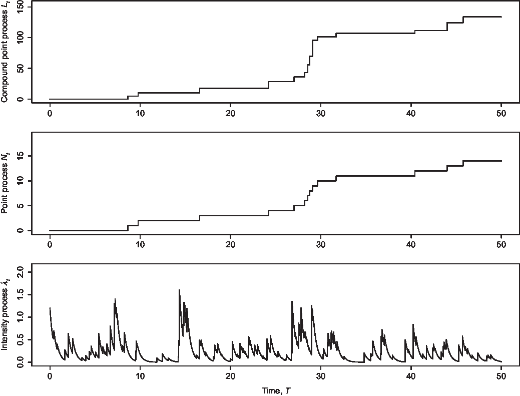
For this purpose, and to make it easier for statistical analysis, further business applications and research, we provide the simulation algorithm for one sample path of the compound dynamic contagion process  $\left(L_{t},N_{t},\lambda _{t}\right) $, with m jump times
 $\{T_{1}^{\ast},T_{2}^{\ast },\ldots ,T_{m}^{\ast }\}$ in the process
 $\lambda _{t}$ (see Figure 1). This algorithm is from Dassios & Zhao (Reference Dassios and Zhao2011) section 5 algorithm, where they have shown how to simulate the dynamic contagion process. We also refer Ogata’s thinning method (Reference Ogata1981) and Møller & Rasmussen (Reference Møller and Rasmussen2005) for Hawkes processes simulations.
Simulated sample path of the compound dynamic contagion process: intensity process  $\protect\lambda_t$, point process
 $N_t$ and compound point process
 $L_t$, with the parameters
 $\left(a;\,\protect\rho;\,\protect\delta;\,\protect\alpha;\,\protect\psi;\,\protect\varsigma;\,c;\,\protect\omega;\,\protect\zeta;\,k;\,\protect\lambda_0\right)=(1;\,3;\,2.5;\,5;\,1;\,5.5;\,3;\,3;\,4;\,6;\,1.2)$.

We provide the simulation algorithm for one sample path of the compound Cox process with shot-noise intensity over a time interval [0, T], adapted the one in Čížek et al. (Reference Cizek, Härdle and Weron2011) (see Figure 2). We omit the simulation algorithm for one sample path of the compound Poisson process at it is trivial.
Simulated sample path of the compound Cox process with shot-noise intensity: intensity process  $\protect\lambda_t$, point process
 $N_t$ and compound point process
 $L_t$, with the parameters
 $\left( \protect\rho;\,\protect\delta;\,\protect\alpha;\,\protect\omega;\,\protect\zeta;\,k;\,\protect\lambda_0\right) = \left(3;\,2.5;\,5;\,3;\,4;\,6;\,1.2 \right) $.

Algorithm 4.1 (The compound dynamic contagion process simulation algorithm).
1. Set the initial conditions
$T_{0}^{\ast }=0,$ $\lambda _{T_{0}^{\ast+}}=\lambda _{0}>a$, and $i\in \{0,1,2,\ldots ,m-1\}$.-
2. Simulate the
$(i+1)^{\text{th}}$ externally excited jump waiting time $E_{i+1}^{\ast }$ by
\begin{equation*}E_{i+1}^{\ast }=-\frac{1}{\rho }\ln U,\text{ \ \ \ \ }U\sim \text{U}(0,1)\end{equation*}
-
3. Simulate the
$(i+1)^{\text{th}}$ self-excited jump waiting time $S_{i+1}^{\ast }$ by
where
\begin{equation*}S_{i+1}^{\ast }=\begin{cases}S_{i+1}^{\ast \left( 1\right)}\wedge S_{i+1}^{\ast \left( 2\right)} & \left(d_{i+1}>0\right) \\[3pt]S_{i+1}^{\ast \left( 2\right)} & \left( d_{i+1}<0\right)\end{cases}\end{equation*}
and
\begin{equation*}d_{i+1}=1+\frac{\delta \ln U_{1}}{\lambda _{T_{i}^{\ast +}}-a} \text{, \ \ \ \ \ \ \ \ }U_{1}\sim \text{U}(0,1)\end{equation*}
\begin{equation*}S_{i+1}^{\ast \left( 1\right) }=-\frac{1}{\delta }\ln d_{i+1}\text{;}\quad S_{i+1}^{\ast \left( 2\right) }=-\frac{1}{a}\ln U_{2}\text{,}\quad U_{2}\sim \text{U}(0,1)\end{equation*}
-
4. Simulate the
$(i+1)^{\text{th}}$ overall jump time $T_{i+1}^{\ast }$ by
\begin{equation*}T_{i+1}^{\ast }=T_{i}^{\ast }+S_{i+1}^{\ast } \wedge E_{i+1}^{\ast }\end{equation*}
-
5. The change at jump time
$T_{i+1}^{\ast }$ in the intensity process $\lambda _{t}$ is given by
where
\begin{equation*}\lambda _{T_{i+1}^{\ast +}}=\begin{cases}\lambda _{T_{i+1}^{\ast -}}+Y_{i+1},\text{ \ \ }Y_{i+1}\sim G(y)\text{ \ }&\left( S_{i+1}^{\ast }\wedge E_{i+1}^{\ast }=S_{i+1}^{\ast }\right) \\\lambda _{T_{i+1}^{\ast -}}+X_{i+1},\text{ \ }X_{i+1}\sim F(x)\text{ \ }&\left( S_{i+1}^{\ast }\wedge E_{i+1}^{\ast }=E_{i+1}^{\ast }\right)\end{cases}\end{equation*}
\begin{equation*}\lambda _{T_{i+1}^{\ast -}}=(\lambda _{T_{i}^{\ast +}}-a)e^{{-\delta(T_{i+1}^{\ast }-T_{i}^{\ast })}}+a\end{equation*}
-
6. The change at jump time
$T_{i+1}^{\ast }$ in the point process $N_{t}$ is given by
\begin{equation*}N_{T_{i+1}^{\ast +}}=\begin{cases}N_{T_{i+1}^{\ast -}}+1 &\left( S_{i+1}^{\ast }\wedge E_{i+1}^{\ast}=S_{i+1}^{\ast }\right) \\[3pt]N_{T_{i+1}^{\ast -}} &\left( S_{i+1}^{\ast }\wedge E_{i+1}^{\ast }=E_{i+1}^{\ast }\right)\end{cases}\end{equation*}
-
7. The change at jump time
$T_{i+1}^{\ast }$ in the compound point process $L_{t}$ is given by
\begin{equation*}L_{T_{i+1}^{\ast +}}=\begin{cases}L_{T_{i+1}^{\ast -}}+\xi _{i+1},\text{ \ }\xi _{i+1}\sim J(\xi ) &\left( S_{i+1}^{\ast }\wedge E_{i+1}^{\ast }=S_{i+1}^{\ast }\right) \\[3pt]L_{T_{i+1}^{\ast -}} &\left( S_{i+1}^{\ast }\wedge E_{i+1}^{\ast }=E_{i+1}^{\ast }\right)\end{cases}\end{equation*}


Algorithm 4.2 (The compound Cox process with shot-noise intensity simulation algorithm).
1. Generate the intensity process
$\lambda _{t}$ over a time interval [0, T] with H(T) jump times $\{t_{1},t_{2},\ldots ,t_{H(T)}\}$:
(i) Simulate H(T) number of jumps by
\begin{equation*}H(T)\sim \mathrm{Poisson}(\rho T)\end{equation*}
-
(ii) Set the initial conditions
$t_{0}=0,$ $\lambda _{0}>0$, and $j\in \{0,1,2,\ldots ,H(T)-1\}$ -
(iii) Conditional on the number of jumps in a Poisson process in the time interval [0,T], the arrival times have a uniform (0, T) distribution. Hence, simulate the
${(j+1)}^{\text{th}}$ conditional jump arrival time $t_{j+1}$ by
\begin{equation*}t_{j+1}\sim \text{U}(0,T)\end{equation*}
-
(iv) The change at jump time
$t_{j+1}$ in the intensity process $\lambda_{t}$ is given by
where
\begin{equation*}\lambda _{t_{j+1}^{+}}=\lambda _{t_{j+1}^{-}}+X_{j+1},\text{ \ \ }X_{j+1}\sim F(x)\end{equation*}
\begin{equation*}\lambda _{t_{j+1}^{-}}=\lambda _{t_{j}^{+}}\,e^{{-\delta (t_{j+1}-t_{j})}}\end{equation*}
-
2. Set the initial conditions
$T_{0}^{\ast }=0$, $\tau =0$, $\lambda^{\#}=\max \left\{ \lambda _{t};\text{ }t\in \lbrack 0,T]\right\} $, and $i\in \{0,1,2,\ldots ,\break K(T)-1\}$, where $K(T)=\max \left\{ i;\text{ }T_{i}^{\ast }<T\right\} $. -
3. Simulate jump times
$\{T_{1}^{\ast },T_{2}^{\ast },\ldots ,T_{K(T)}^{\ast}\}$ by the following steps:
-
(i) Simulate the jump waiting time
$E^{\ast }$ with intensity $\lambda ^{\#}$ by
\begin{equation*}E^{\ast }=-\frac{1}{\lambda ^{\#}}\ln U_{1},\text{ \ \ \ \ }U_{1}\sim \text{U}(0,1)\end{equation*}
-
(ii) Simulate the candidate jump time
$\tau $ by
\begin{equation*}\tau =\tau +E^{\ast }\end{equation*}
-
(iii) The jump time
$T_{i+1}^{\ast }$ is given by $\tau $ if
where
\begin{equation*}U_{2}\leq \dfrac{\lambda _{\tau }}{\lambda ^{\#}},\text{ \ \ \ \ }U_{2}\sim\text{U}(0,1)\end{equation*}
\begin{equation*}\lambda _{\tau }=\lambda _{t^{\ast }}\,e^{{-\delta (\tau -t^{\ast })}}\text{\ \ and \ \ }t^{\ast }=\max \left\{ t_{s};\text{ }t_{s}<\tau ,\text{ }s\in\{0,1,\ldots ,H(T)\}\right\}\end{equation*}
-
-
4. The change at
$T_{i+1}^{\ast }$ in the point process $N_{t}$ is given by
\begin{equation*}N_{T_{i+1}^{\ast +}}=N_{T_{i+1}^{\ast -}}+1\end{equation*}
-
5. The change at
$T_{i+1}^{\ast }$ in the compound point process $L_{t}$ is given by
\begin{equation*}L_{T_{i+1}^{\ast +}}=L_{T_{i+1}^{\ast -}}+\xi _{i+1},\ \xi _{i+1}\sim J(\xi)\end{equation*}


Value-at-risk (VaR)

Tail conditional expectation (TCE or TailVaR)

Let us now illustrate the calculations of two risk measures. For  $F\left(x\right) $, we use an exponential distribution, i.e.,
 \begin{equation*}1-e^{-\alpha x}\text{, \ }\alpha >0\end{equation*}
and for G(y), we use a Loggamma distribution with probability density, i.e.,
 \begin{equation*}\frac{\varsigma ^{c}}{\psi \Gamma \left( c\right) }\left\{ \ln \left( \frac{y}{\psi }+1\right) \right\} ^{c-1}\left( \frac{y}{\psi }+1\right)^{-\varsigma -1},\psi >0,\ \varsigma >0\ \ \text{and}\ \ c>0\end{equation*}
to capture the effect of sudden increases of the intensity, i.e., after-incidents/shocks driven by initial incidents/shocks. For  $J(\xi ),$ we use a Pareto distribution with probability density, i.e.,
 \begin{equation*}\frac{\Gamma \left( \omega +k\right) \text{ }\zeta ^{\omega }\text{ }\xi^{k-1}}{\Gamma \left( \omega \right) \text{ }\Gamma \left( k\right) \text{ }\left( \zeta +\xi \right) ^{\omega +k}},\ \omega >0,\ \zeta >0\ \ \text{and}\ \ k>0\end{equation*}
Hence, the parameter values to simulate the compound processes and calculate two risk measures are
 \begin{eqnarray*}a &=&1,\text{ }\rho =3,\text{ }\delta =2.5,\text{ }\alpha =5,\text{ }\psi =1,\text{ }\varsigma =5.5\text{, }c=3 \\\omega &=&3,\text{ }\zeta =4,\text{ }k=6\text{\ and }\lambda _{0}=1.2\end{eqnarray*}
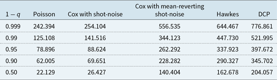
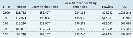
Simulations were run with 20,000 paths for each compound process using R. Tables 1 and 2 show the values of VaR and TCE at confidence level q at time  $t=10$.
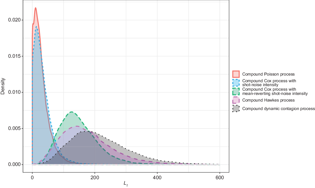
Remark 4.1. Tables 1 and 2 show that two risk measures significantly increase when changing  $N_{t}$ from the Cox process with shot-noise Poisson intensity to a generalised Hawkes process due to self-excited jumps, and to the dynamic contagion process due to both externally excited jumps and self-excited jumps (see Figure 3).
Density plots of the compound point processes  $L_t$: compound Poisson process, compound Cox process with shot-noise intensity, compound Cox process with mean-reverting shot-noise intensity, compound Hawkes process and compound dynamic contagion process at
 $t = 10$ with the parameters given as
 $\protect\eta=0.24$ and
 $\left(a;\,\protect\rho, \protect\delta;\,\protect\alpha;\,\protect\psi;\protect\varsigma;\,c;\,\protect\omega;\,\protect\zeta;\,k;\,\protect\lambda_0\right) = (1;\,3;\,2.5;\,5;\,1;\,5.5;\,3;\,3;\,4;\,6;\,1.2)$.

5 Conclusion
We have reviewed and studied the compound processes of the Poisson, Cox, Hawkes, shot-noise Poisson and dynamic contagion process. The analytic expressions of the Laplace transforms of these processes and their moments have been presented, which have the potential to be applicable to a variety of problems in economics, finance and insurance. To make it easier for statistical analysis, further business applications and research, we provided the simulation algorithm for compound dynamic contagion process and compound Cox process with shot-noise intensity, respectively. We also made numerical comparisons of VaR and TCE as an application of the compound processes.
This work can be extended by incorporating interarrival jump times with renewal processes, where the moments of renewal shot-noise processes have been shown in Jang et al. (Reference Jang, Dassios and Zhao2018a) and Dassios et al. (Reference Dassios, Jang and Zhao2015) studied a risk model with renewal shot-noise Cox process.
Given the current COVID-19 pandemic, a significant challenge ahead is to model the number of losses and their magnitudes from the interruption of businesses and its economic impact. Public and private sector organisations face unexpected credit risks resulting from pandemic events. Taking into account the impact of pandemic risk in modelling the price and stochastic volatility of an asset will be the new normal post-COVID-19. Insurers will need tools to deal with the challenge of new risk dynamics arising from pandemic events. Work-from-home arrangements can expose corporate networks to the vulnerabilities found in home Wi-Fi routers as cyber risks. Hence, when credit, cyber, economic, financial, insurance and other risks are extreme/non-extreme losses in practice (i.e. their distributions are heavy-tailed/light-tailed), reviewed point processes can be used for these risks with flexibility.
We hope that findings of this paper provide academics/practitioners with feasible models to count numbers of claims/losses and their aggregation. We also recommend the use of more multivariate models of these processes to deal with the arrival of multiple, catastrophic and contagious losses accommodating the interdependence between risks.
Acknowledgements
Rosy Oh’s research was supported by Basic Science Research Program through the National Research Foundation of Korea (NRF) funded by the Ministry of Education (Grant No. 2019R1A6A1A11051177 and 2020R1I1A1A01067376).
Appendix A Proof of Theorem 3.1
Consider a function  $f\left( \lambda ,n,l,t\right) $ with an exponential affine form
 \begin{equation*}f\left( \lambda ,n,l,t\right) =\theta ^{n}e^{-\nu l}e^{-B\left( t\right)\lambda }e^{C(t)}\end{equation*}
substitute into  $\mathcal{A}$
 $f=0$ in (16), we have
 \begin{equation*}-\lambda B^{\prime }\left( t\right) +C^{\prime }\left( t\right) +\lambda\left[ \theta \text{ }\hat{g}\left\{ B\left( t\right) \right\}\text{ }\hat{j}\left( \nu \right) \right] +\delta \left(a-\lambda \right) \left\{ -B\left( t\right) \right\} +\rho \left[ \hat{f}\left\{ B\left( t\right) \right\} -1\right] =0\end{equation*}
 \begin{equation*}\left[ {-}B^{\prime }\left( t\right) +\delta B\left( t\right) +\theta \text{ }\hat{g}\left\{ B\left( t\right) \right\} \text{ }\hat{j}\left( \nu \right) -1\right] \lambda +\left[ C^{\prime }\left(t\right) +\rho \text{ }\hat{f}\left\{ B\left( t\right) \right\}-\rho -\delta aB\left( t\right) \right] =0 \notag\end{equation*}
Since this equation holds for any l, n and  $\lambda $, it is equivalent to solving two separated equations, i.e.,
 \begin{equation}-B^{\prime }\left( t\right) +\delta B\left(t\right) +\theta \text{ }\hat{g}\left\{ B\left( t\right)\right\} \text{ }\hat{j}\left( \nu \right) -1=0 \end{equation}
 \begin{equation}C^{\prime }\left( t\right) +\rho \text{ }\hat{f}\left\{ B\left(t\right) \right\} -\rho -\delta aB\left( t\right) =0 \end{equation}
We have two ODEs of (A.1) and (A.2) with the boundary condition  $B\left(T\right) =\upsilon $. By (A.2) with boundary condition
 $C\left( 0\right)=0,$ the integration of (21) follows. Since
 $\theta ^{N_{t}}e^{-\nu L_{t}}e^{-B\left( t\right) \lambda _{t}}e^{C(t)}$ is a
 $\Im $-martingale by the property of the infinitesimal generator, we have
 \begin{equation*}\mathbb{E}\left[ \theta ^{N_{T}}e^{-\nu L_{T}}e^{-B(T)\lambda _{T}}e^{C(T)}\mid \Im_{t}\right] =\theta ^{N_{t}}e^{-\nu L_{t}}e^{-B(t)\lambda _{t}}e^{C(t)}\notag\end{equation*}
Then, by the boundary condition  $B\left( T\right) =\upsilon ,$ (19) follows.
Appendix B Proof of Theorem 3.2
By setting  $t=0$ and
 $\theta =1$ in (19), we have
 \begin{equation}\mathbb{E}\left[ e^{-\nu L_{T}}e^{-\upsilon \lambda _{T}}\mid \Im _{0}\right]=e^{-B(0)\lambda _{0}}e^{-C(T)} \end{equation}
where B(0) is uniquely determined by the non-linear ordinary differential equation (ODE)
 \begin{equation}-B^{\prime }\left( t\right) +\delta B\left( t\right) +\hat{g}\left\{ B\left( t\right) \right\} \text{ }\hat{j}\left( \nu\right) -1=0 \end{equation}
with boundary condition  $B\left( T\right) =\upsilon $. (B.2) can be solved, under the condition
 $\delta >$
 $\hat{j}\left( \nu \right) $
 $\mu _{1_{G}}$, by the following steps (1)–(7):
(1) Let us set
$B(t)=\Psi (T-t)=\Psi (\tau ).$ Then it becomes
(B.3)with initial condition
\begin{equation}\frac{d\Psi (\tau )}{d\tau }=1-\delta B(t)-\hat{g}\left\{B(t)\right\} \hat{j}\left( \nu \right) =1-\delta \Psi (\tau )-\hat{g}\left\{ \Psi (\tau )\right\} \hat{j}\left(\nu \right) =\!:\,f(\Psi ) \end{equation}
$\Psi (0)=\upsilon ;$ we define the right-hand side as the function, $f(\Psi )$.
-
(2) Under the condition of
$\delta >$ $\hat{j}\left( \nu \right) $ $\mu _{1_{G}}$, we have
then
\begin{equation*}\frac{\partial f(\Psi )}{\partial \Psi }=\hat{j}\left( \nu\right) \int\limits_{0}^{\infty }ye^{-\Psi \text{ }y\text{ }}dG(y)-\delta\text{ }\leq \text{ }\hat{j}\left( \nu \right)\int\limits_{0}^{\infty }\text{ }ydG(y)-\delta =\text{ }\hat{j}\left( \nu \right) \mu _{1_{G}}-\delta <0,\text{ \ for }\Psi \geq 0\end{equation*}
$f(\Psi )<0$ for $\Psi >0$.
-
(3) (B.3) can be written as
Integrate both sides from time 0 to
\begin{equation*}\frac{d\Psi (\tau )}{\delta \Psi (\tau )+\text{ }\hat{j}\left(\nu \right) \hat{g}\left\{ \Psi (\tau )\right\} -1}=-d\tau\end{equation*}
$\tau $ with initial condition $\Psi(0)=\upsilon >0,$ then we have
where
\begin{equation*}\int\limits_{\Psi }^{\upsilon }\left[ \frac{1}{\delta \text{ }u+\text{ }\hat{j}\left( \nu \right) \hat{g}\left( u\right) -1}\right] du=\tau\end{equation*}
$\Psi \geq 0.$ Now we define the left-hand side as the function
Then, we have
\begin{equation*}\mathcal{G}_{\upsilon ,\nu }(\Psi )=\!:\,\int\limits_{\Psi }^{\upsilon }\left[\frac{1}{\delta \text{ }u+\text{ }\hat{j}\left( \nu \right)\hat{g}\left( u\right) -1}\right] du\end{equation*}
which is the time difference between T and t and it is obvious that
\begin{equation*}\mathcal{G}_{\upsilon ,\nu }(\Psi )=\tau \text{ }(=T-t)\end{equation*}
$\Psi \rightarrow \upsilon $ when $\tau $ $(\!=T-t)\break\rightarrow 0.$
-
(4) As
$\delta -$ $\hat{j}\left( \nu \right) \mu _{1_{G}}>0$ by convergence test, we have
so
\begin{equation*}\int\limits_{0}^{\upsilon }\left[ \frac{1}{\delta \text{ }u+\text{ }\hat{j}\left( \nu \right) \hat{g}\left( u\right) -1}\right]du=\infty\end{equation*}
$\Psi \rightarrow 0$ when $\tau \rightarrow \infty .$ The integrand is positive in the domain $u\in (0,\upsilon ]$ and also for $\Psi \leq \upsilon $. The function $\mathcal{G}_{\upsilon ,\nu }(\Psi )$ is strictly decreasing, therefore
is a well-defined (monotone) function and its inverse function
\begin{equation*}\mathcal{G}_{\upsilon ,\nu }(\Psi )=\tau :\,(0,\upsilon ]\rightarrow \lbrack0,\infty )\end{equation*}
exists.
\begin{equation*}\mathcal{G}_{\upsilon ,\nu }^{-1}(\tau )=\Psi :\,[0,\infty )\rightarrow(0,\upsilon ]\end{equation*}
-
(5) The unique solution is found by
and hence B(0) is obtained,
\begin{equation*}\Psi \left( \tau \right) =\Psi \left( T-t\right) =B(t)=\mathcal{G}_{\upsilon,\nu }^{-1}(\tau )=\mathcal{G}_{\upsilon ,\nu }^{-1}(T-t)\end{equation*}
\begin{equation*}B(0)=\Psi \left( T\right) =\mathcal{G}_{\upsilon ,\nu }^{-1}(T)\end{equation*}
-
(6) Now C(T) is determined by
By the change of variable
\begin{equation*}C(T)=\rho \int\limits_{0}^{T}\left[ 1-\hat{f}\left\{ \mathcal{G}_{\upsilon ,\nu }^{-1}(\tau )\right\} \right] d\tau +a\delta\int\limits_{0}^{T}\mathcal{G}_{\upsilon ,\nu }^{-1}(\tau )d\tau\end{equation*}
$\mathcal{G}_{\upsilon ,\nu }^{-1}(\tau )=u,$ we have $\tau =\mathcal{G}_{\upsilon ,\nu }^{-1}(u)$, and
\begin{equation*}\int\limits_{0}^{T}\mathcal{G}_{\upsilon ,\nu }^{-1}(\tau )d\tau=\int\limits_{\mathcal{G}_{\upsilon ,\nu }^{-1}(0)}^{\mathcal{G}_{\upsilon,\nu }^{-1}(T)}u\frac{\partial \tau }{\partial u}du=\int\limits_{\mathcal{G}_{\upsilon ,\nu }^{-1}(T)}^{\upsilon }\left\{ \frac{u}{\delta \text{ }u+\text{ }\hat{j}\left( \nu \right) \hat{g}\left(u\right) -1}\right\} du\end{equation*}
-
(7) Finally, substitute B(0) and C(T) into (B.1) and the result follows.


Appendix D Proof of Theorem 4.1
Setting  $\mathcal{A}$
 $f\left( \lambda ,n,l,t\right) =l$ in (16), we have
 \begin{equation*}\mathcal{A}\text{ }l=\mu _{1_{J}}\lambda\end{equation*}
As  $L_{t}-L_{0}-\int\limits_{0}^{t}\mathcal{A}$
 $l_{s}ds$ is a
 $\Im _{t}$ -martingale, we have
 \begin{equation*}\mathbb{E}\left\{ L_{t}-\int\limits_{0}^{t}\mathcal{A}\text{ }l_{s}ds\mid \lambda_{0}\right\} =L_{0}\end{equation*}
Hence
 \begin{equation*}\mathbb{E}\left( L_{t}\mid \lambda _{0}\right) =L_{0}+\mathbb{E}\left\{ \int\limits_{0}^{t}\mathcal{A}\text{ }l_{s}ds\mid \lambda _{0}\right\} =L_{0}+\mu_{1_{J}}\int\limits_{0}^{t} \mathbb{E}\left( \lambda _{s}\mid \lambda _{0}\right) ds\end{equation*}
From Proposition 3.1 in Jang & Dassios (Reference Jang and Dassios2013), the conditional expectation of the process  $\lambda _{t}$ given
 $\lambda _{0}$ at time
 $t=0$ is given by
 \begin{equation*}\mathbb{E}\left( \lambda _{t}\mid \lambda _{0}\right) =\lambda _{0}e^{-\left( \delta-\mu _{1_{G}}\right) t}+\frac{\mu _{1_{F}}\text{ }\rho +a\delta }{\delta-\mu _{1_{G}}}\left( 1-e^{-\left( \delta -\mu _{1_{G}}\right) t}\right)\!,\text{ \ \textit{for} }\delta \neq \mu _{1_{G}} \notag\end{equation*}
and (27) follows.