

Introduction
Digital elevation models (DEMs) find a growing range of applications, such as terrain visualisation, planning and maintenance of infrastructure, land-use mapping, hydrological characterisation, orthorectification of airborne and satellite imagery, energy-balance modelling of glaciers, and detection of topographic change over time (Racoviteanu and others Reference Racoviteanu, Manley, Arnaud and Williams2007; Jones and others Reference Jones, Poole, O'Daniel, Mertes and Stanford2008; Fisher and Tate Reference Fisher and Tate2006). DEMs have traditionally tended to be supplied by national mapping agencies, often at some expense, although researchers have increasingly been producing their own, using a variety of methods including field survey, stereophotography, stereo radargrammetry, interferometric synthetic aperture radar and LiDAR.
Since the early 1990s, global, or near global, DEMs have been freely available for most or all of the Earth's land surface at a resolution of 1 km or finer. These have proved to be a hugely valuable resource for research. At first these global DEMs were derived from existing topographic maps: the GTOPO30 DEM, described briefly below, was the first example of this type of DEM, and the NOAA GLOBE project is a more recent example. At the beginning of the new millennium, however, a new type of global, or near global, DEM became available, generated from satellite data. This was the shuttle radar topography mission (SRTM, also outlined below), which provided data for most of the Earth's land surface at an unprecedentedly high spatial resolution. Satellite-derived DEMs offer substantial advantages compared with global DEMs compiled from existing topographic maps, notably spatial and temporal consistency and a recent date of compilation.
Since 2009, a new global satellite-derived DEM has become freely available: the global DEM (GDEM), generated from data collected by the ASTER (advanced spaceborne thermal emission and reflection radiometer) instrument carried on board the Terra satellite. As well as having a generally higher spatial resolution than SRTM, it extends to a latitude of 83 °N whereas SRTM data extend only to a latitude of 60°. Thus, GDEM represents the first truly Arctic global DEM derived from satellite data. However, little has so far been published on the accuracy of GDEM. It is therefore of some interest to assess its accuracy in a number of differentiated Arctic locations, and that is the aim of this paper.
Characteristics of a DEM
The fundamental characteristic of a DEM is its coverage; simply the area of the Earth's surface represented by it. In a straightforward way the DEM may also be fixed in time, through its date of compilation or acquisition. spatial resolution is a more difficult concept to define. All the DEMs considered in this paper are in raster format, so the concept of a horizontal sampling (sometimes called ‘posting’) interval is meaningful. However, the spatial resolution may be coarser than implied by the sampling interval. Many DEMs show spatial correlation of errors (Fisher Reference Fisher1998; Fisher and Tate Reference Fisher and Tate2006; Erdogan Reference Erdogan2010) for a variety of reasons, and the sampling interval may fail to reflect this correlation. We may also need to consider the horizontal accuracy of the DEM, that is the typical horizontal displacement between a point as represented in the DEM and its true location. This is equivalent to the concept of georeferencing accuracy. Analogous considerations apply to the height information contained in the DEM, which can be characterised by its precision and its accuracy. Finally, we can try to represent the nature of the errors in the DEM by characterising its artefacts.
The GTOPO30 DEM can be considered in these terms. It is a truly global DEM in the sense that it represents the whole of the Earth's surface. Ocean surfaces are defined to have an elevation of zero. The sample interval is 30 arcseconds, that is roughly 0.93 km in latitude and (0.93 cos φ) km in longitude, where φ is the latitude, and the vertical precision is 1 m. The sampling interval of 30 arcseconds and the global coverage implies that the entire DEM is represented by just under one billion points, and since each elevation can be represented by a 2 byte number the total uncompressed data volume is around 1.74 gigabytes. The spatial resolution and height accuracy of the dataset are variable: it was compiled from eight different DEMs. In the Arctic, most of the data are derived from the digital chart of the world (DCW), digital terrain elevation data (DTED) and the USGS 1-degree DEM. While the last two have sampling intervals of 3 seconds of arc (around 90 m in latitude), the DCW was digitised from maps having a scale of 1:1 million and a contour interval of 1000 feet (305 m) (GTOPO30 Documentation 2011). It is perhaps reasonable to state that the elevation accuracy of GTOPO30 ranges from around 20 to above 100 m. Artefacts in GTOPO30 arise mainly from the low precision of the input elevation data, and from forming a mosaic of different DEMs.
The SRTM was a space shuttle mission flown during February 2009 (Shuttle Radar Topography Mission 2011). The latitudinal coverage of the data is from 56 °S to 60 °N and, like GTOPO30, data are available for land covered areas (a few water covered areas were also included). The sampling interval for most parts of the world is 3 seconds (about 90 m in latitude) although for the USA the sampling interval is 1 second (30 m). The entire DEM is represented by around 2 × 10¹⁰ points and a data volume of around 100 GB (ignoring repeat coverage of some locations). The data are distributed in 1° tiles, each tile containing 1201 × 1201 elevations. Unlike GTOPO30, the spatial resolution and height accuracy are spatially uniform, the latter being around 10 m. The principal artefact in the SRTM DEM is ‘voids’, or areas of missing data. Although these are not generally a major problem, they are more numerous in areas of high relief.
GDEM
The GDEM was developed jointly by the Japanese Ministry of Economy, Trade and Industry (METI) and by NASA. It uses stereogrammetric data from the ASTER instrument carried on board the Terra satellite since 2000. Automated processing of the stereo images, without manual intervention, is used to generate DEMs and surface elevations are based on the average of several DEMs. Version 1 of the GDEM product was released in June 2009. The data are distributed in 1° square tiles at a sampling interval of 1 second, so each tile consists of 3601 × 3601 points. The elevation precision is 1 m and the nominal accuracy of the product is stated to be 20 m in elevation and 30 m in horizontal position. The spatial coverage is between 83° north and south latitudes, potentially including a huge area of the Arctic (and indeed the Antarctic) inaccessible to the SRTM. It is a large dataset: in total it consists of around 22600 tiles, each of which consists of just under 50 MB, so the total data volume is around 1 terabyte. Version 1 of the GDEM, released in 2009, is described as preliminary and of research grade. The aim of the work described in this paper is to assess its likely utility for arctic research.
Methods and test sites
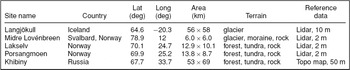
GDEM data were downloaded for five Arctic test sites, in Iceland, Svalbard, mainland Noway, and Russia, detailed below (Table 1). The test sites were all selected on the basis that they were areas of significant research interest at the Scott Polar Research Institute so that their general characteristics were well understood, and they provided a range of surface cover types including ice, tundra, boreal forest and bare rock. Reference elevation data were available for all five of the test sites. In four cases the data were provided through airborne LiDAR campaigns, with elevation accuracies of significantly better than 1 m and spatial resolutions of 2 m or 10 m. The one exception to this was the Russian test site where the only topographic data available for comparison were derived by digitisation of a paper topographic map at a scale of 1:100,000. The map, compiled by the Russian General Staff in 1981, had a contour interval of 20 m. All the reference DEMs were supplied in UTM projection on the WGS84 datum.
Test sites. The first two columns identify the name and country, while the next two give a nominal location of the site. The column ‘area’ shows the dimensions of the bounding rectangle around the study site, with the east-west dimension shown first. ‘Terrain’ shows the main land cover types present in the test site and the last column shows the type of reference data, together with its horizontal sampling interval, used to compare the GDEM data against.

GDEM data were acquired for each of the test sites. In all cases, the GDEM data consisted of two 1° tiles, one containing the elevation data and the other containing a quality indicator which, in all cases, was the stacking number, that is the number of independent estimates of the elevation contributing to the average. Both tiles were reprojected and resampled to the UTM projection and spatial resolution of the corresponding reference data. The reprojection algorithm took no account of the altitude, that is the DEMs were reprojected in the same way as an image would be. Nearest neighbour resampling was employed in all cases. The decision to resample the GDEM data to the resolution of the reference data was a pragmatic one, since the reference datasets had widely differing sampling intervals. It clearly resulted in massive oversampling of the GDEM data where they were compared against the 2 m LiDAR data, and this dictated the choice of nearest neighbour resampling of the GDEM to avoid introducing spurious spatial resolution at scales finer than 30 m.
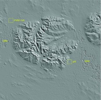
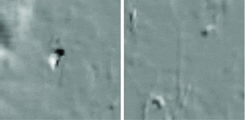
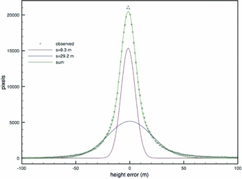
Fig. 1 shows the GDEM data for the Khibiny test site. The GDEM data are not masked for areas of water, and the test site of Fig. 1 includes two large lakes over which the DEM is clearly unsatisfactory. The figure also illustrates two common types of artefact, termed ‘pits’ and ‘mole runs’ (ASTER GDEM Validation Team 2009). Enlargements of these features are shown in Fig. 2. Pits (and bumps) are point like anomalies and mole runs are linear anomalies, most probably related to the boundary between areas with different stacking numbers. A preliminary assessment of the errors in the DEM shown in Fig. 1 was performed by calculating the difference between the GDEM data and the corresponding reference data, excluding water areas. After subtracting the mean from the difference to allow for any possible difference in datum, and also for errors introduced by the resampling process, the histogram of the residual errors was calculated. This is shown in Fig. 3.
Slope-shaded GDEM of the Khibiny test site.

Enlargements of the artefacts identified in fig. 1. Left: pit; right: mole run.

Histogram of height error in the DEM of figure 1, fitted to the sum of two Gaussian distributions.

The histogram of height errors is not well described by a single Gaussian distribution but much better described as the sum of two Gaussians, with standard deviations of around 10 m and 30 m respectively. These are tentatively identified as the distributions of ‘normal errors’ and ‘blunders’ respectively. Although not conclusive, the data of Fig. 3 are at least suggestive of the existence of two populations. Detailed analysis of the spatial distribution of errors in the DEMs from each of the five test sites was carried out as follows. First, the mean of the GDEM data was adjusted to correspond to that of the reference data, again to allow for the possibility of a difference in datum between the two datasets. Then two intersecting linear transects were defined, by eye and roughly orthogonal, and the elevation profiles h(x) were calculated for these transects from both the GDEM and the reference data. For each transect, the error transect e(x) was defined as

and this was used to calculate the error semivariance

where the angle brackets denote averaging over all x′ along the transect. Although the use of semivariances is well established in geostatistics, it does not appear to have found much application to the analysis of DEM errors, although it would appear rather well suited to this task. The semivariance was described through

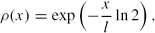
where σ is the standard deviation of the error and ρ(x) is its autocorrelation function. Three candidate models of the autocorrelation function (acf) were tried: the negative exponential model
the Gaussian model
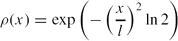
and the Lorentzian (or Cauchy) model
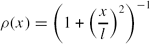
In each case the acf is parameterised by the correlation length l, defined as the length scale at which the acf falls to ½. The method of least squares was used to determine which of the three models of acf fitted the data best, and the appropriate values of σ and l. None of these models has a particular physical basis, and they have been chosen as examples of simple monotonically increasing functions. Comparison between the fits gives some indication of the robustness of the calculated values of σ and l.
In addition, the mean value n of the stacking number was calculated for each transect.
Results
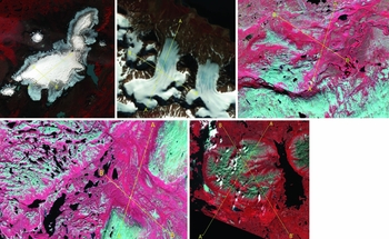
Fig. 4 shows the locations of the transects in each of the test sites. In each case the transects have been superimposed on false colour infrared (FCIR) composites of extracts of Landsat images which were used to guide the choice of transects. The Landsat images were all downloaded from the University of Maryland's global land cover facility.
FCIR Landsat image extracts showing the locations of the transects analysed in this paper. The images are presented in the same order as in table 1. In each case transect 1 runs from A to A′ and transect 2 from B to B′.

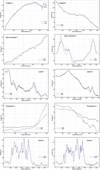
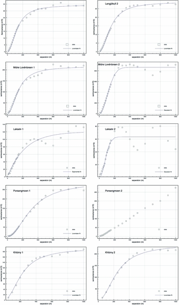
The elevation profiles for each transect are shown in Fig. 5, and the corresponding error semivariograms are shown in Fig. 6, together with the best fitting model selected from amongst equations (4a), (4b) and (4c). No model could meaningfully be fitted to the results for transect 2 from the Porsangmoen test site. Fig. 6 shows oscillatory behaviour in some of the semivariograms. For this reason, a ‘wave-hole-effect’ autocorrelation function (equation 4d) was also tested.
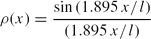
This did not, however, improve the fit in any case.
Elevation transects from GDEM and reference data.

Semivariograms of GDEM error with best-fitting models.

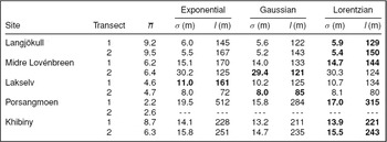
The results of this analysis are summarised in Table 2, which shows that the estimated values of σ and l are in most cases not strongly dependent on the particular model of autocorrelation function. This lends some confidence to the estimates of these values. In most cases the best fitting model is, qualitatively, a good fit to the observed semivariogram, although as noted earlier some of the semivariograms also exhibit some unmodelled oscillatory behaviour.
Mean stacking number n and error parameters for each transect. - - - denotes that values could not be meaningfully determined. Bold entries show the best fitting model.

The GDEM transects over Langjökull are impressively faithful. Fig. 5 shows some large errors, of the order of 100 m, in transect 1. These are all in places where the stacking number n is less than 5. Elsewhere, however, the GDEM transects appear to be well characterised by the rms error of 5–6 m with a correlation length of 130–150 m. The two transects over Midre Lovénbreen show rather different behaviour. Transect 1, which is mainly along the length of the glacier, follows the topography reasonably closely, with an rms error of around 15 m and maximum errors of around 50 m. Transect 2, on the other hand, is transverse to the glacier and includes a significant amount of exposed rock. The rms error is about twice as great in this case, although the largest errors are still mostly around 50 m. Most of the large errors occur on the steepest terrain, again where n is below about 5. The correlation length of the errors is similar to that observed for Langjökull.
The data from Lakselv transect 1 show a broadly similar pattern, with maximum errors of around 50 m over the steepest slopes. Transect 2 shows considerably smaller errors, and a significantly shorter correlation length. Both the Lakselv transects are characterised by rather low values of the stacking number n. The two Porsangmoen transects have even lower values of n, averaging below 3, and the GDEM transects are very poor. While it was possible to fit a model to the error semivariogram of transect 1, and hence to estimate values of σ and l, these values are not particularly useful. It did not prove possible to fit a model to the semivariogram from transect 2, and the simplest statement is probably that the GDEM algorithm has failed to produce a valid DEM for the Lakselv test site.
The final test site, Khibiny, shows remarkable fidelity between the GDEM and reference transects. This is in part, however, a consequence of the high degree of relief in the test site: in fact transect 2 shows an error over 100 m at one location. The estimates of σ and l for the Khibiny transects are not directly comparable to those from the other test sites, since the reference data have been generated from a paper map and will have a significantly poorer spatial resolution. Thus the values of 14–16 m for σ and of 220–240 m for l may be taken as upper limits to the true values.
Discussion
Although the range of test sites examined here is not large, some patterns are suggested by the results. The correlation length of elevation errors is typically around 130 m, similar to the estimated figure of 100–120 m (ASTER GDEM validation team 2009). This is a more meaningful figure for the spatial resolution of the data than the 1-arcsecond sampling interval. The Lorentzian model usually appears to provide a reasonable description of the spatial distribution of the elevation errors. The rms error appears to be rather strongly dependent on the stacking number n, which is not particularly surprising if the errors in each of the n DEMs contributing to the GDEM product can be regarded as independent of the others. The limited range of data examined here suggests that the DEM is reliable only if n > 6, approximately, while the DEMs generated from n < 3 contained major errors. This is a particularly interesting result, suggesting that the error in the DEM cannot simply be modelled as proportional to n −1/2. Slope appears to affect accuracy, again not particularly surprisingly, though the stacking number tends to be lower on steeply sloping terrain so it is possible that the effect of slope on accuracy is entirely represented by the effect of n. There is no strong evidence that the nature of the land cover (whether snow, ice, bare rock, tundra or forest) affects the accuracy, although again any such influence may be manifested through an effect on n. For stacking number n greater than about 6, the rms error appears to be typically 5–10 m, with maximum errors of around 50 m. Comparison of GDEM data with over 13,000 ground control points across the USA (ASTER GDEM validation team 2009) showed an rms error of about 9 m, consistent with the figure reported here.
These results suggest, firstly, that the general performance figures estimated for ASTER GDEM (ASTER GDEM validation team 2009) on the basis of measurements from the USA are also valid for the terrestrial Arctic and, secondly, that GDEM data have a useful role to play in Arctic research even while they are still at their preliminary, version-1, stage. As noted earlier, GDEM extends the coverage of satellite derived DEMs from a latitude of 60° to 83°, to include almost all of the terrestrial Arctic. The QA data, in the form of the stacking number, give a strong indication of the likely usefulness and accuracy of the DEM. The ASTER GDEM validation report shows (ASTER GDEM validation team 2009) the global distribution of stacking number in the current GDEM product. In the latitudinal band between 60 and 83 °N this exceeds 6 in most of Alaska, the Canadian north, Iceland, Scandinavia, the islands of the high Arctic and significant parts of northern Asia. In Greenland however, the stacking number is below 6 over most of the ice sheet (as it is over most of the Antarctic ice sheet, in fact).
Apart from questions about its accuracy and the presence of artefacts, one criticism of the GDEM dataset is that it does not include a water mask. This is however fairly easily remedied, for example through the classification of satellite imagery (and clearly if GDEM coverage is available then so must be ASTER imagery). Potentially more significant is the ambiguity over the date of acquisition. Images used in constructing the GDEM could have been acquired at any time between the years 2000 and 2008. This is clearly problematic if the topography is expected to vary over time, as would be the case for a glacier. However, the contribution of this uncertainty to an estimate of glacier mass balance can be estimated.
The ASTER GDEM dataset should also be placed in the context of future developments. We may confidently expect that GDEM will itself be refined and improved, but there other initiatives directed towards the development of accurate, high resolution DEMs with near global coverage. A number of countries are currently engaged in, or have already completed, programmes to acquire LiDAR DEMs at a spatial resolution of 1 m. In an arctic context, Sweden and Finland have programmes currently in progress. Other national programmes exist, for example the Canadian plan to use Radarsat-2 SAR data to map the entire country (CSA Mapping 2011). By 2016, the TanDEM-X/TerraSAR-X project (DLR Earth Observation 2011) is scheduled to have mapped the whole of the Earth's surface using InSAR at a spatial resolution of 12 m and with a vertical accuracy of 2 m.
Conclusions
While the ASTER GDEM product is currently supplied on the basis that it is ‘experimental’ and of ‘research grade’, it evidently fills a significant gap in the availability of high resolution DEM data, especially at high latitudes, and it can be used with caution. Its elevation accuracy is typically 5–10 m (although absolute accuracy was not investigated in this study) and its spatial resolution is of the order of 100 m. The stacking number appears to be a good indicator of the likely quality, and the data examined here suggest that provided this is at least 6 the data should be reliable. The provision of global covcrage high resolution DEM data is likely to improve significantly over the next few years, not least through improvements to the GDEM product itself, but for now, in the early 2010s, GDEM is likely to find extensive use in Arctic (and other) research.
Acknowledgements
ASTER GDEM data are a product of METI and NASA. Data were downloaded from Earth Observing System Data and Information System (EOSDIS). 2009. Earth Observing System ClearingHOuse (ECHO) / Warehouse Inventory Search Tool (WIST) Version 10.X [online application]. Greenbelt, MD: EOSDIS, Goddard Space Flight Center (GSFC) National Aeronautics and Space Administration (NASA) (URL: https://wist.echo.nasa.gov/api/). Landsat satellite imagery was downloaded from the Global Land Cover Facility, University of Maryland (URL: http://www.glcf.umd.edu). Data processing was conducted on an Apple Macintosh computer using free software: ImageJ (Rasband Reference Rasband1997) and Multispec (Biehl and Landgrebe Reference Biehl and Landgrebe2002). This paper is a product under the IPY core project PPS Arctic.