1. Introduction
High-fidelity experimental measurements with fine spatial and temporal resolution are essential in fluid mechanics research, e.g. to uncover new physical mechanisms, to validate theoretical models and to provide data for model development (Tropea, Yarin & Foss Reference Tropea, Yarin and Foss2007). In this context, experimental fluid mechanics relies heavily on particle image velocimetry (PIV) and its tomographic and volumetric variants to visualise and quantify complex flow phenomena over extended spatial domains. However, practical constraints on camera resolution, optical access, particle seeding and light intensity impose a fundamental trade-off among field of view, spatial resolution and temporal sampling rate (Raffel et al. Reference Raffel, Willert, Scarano, Kähler, Wereley and Kompenhans2018). As a result, many laboratory measurements are strongly under-resolved in either space or time, or both: small-scale vortices and shear layers are filtered out by finite interrogation windows (Lavoie et al. Reference Lavoie, Avallone, De Gregorio, Romano and Antonia2007), and high-frequency dynamics is attenuated or aliased when the sampling interval approaches or exceeds the characteristic time scales of the flow (Manovski et al. Reference Manovski, Vinuesa, Schlatter and Schlatter2025). These limitations are particularly severe in turbulent or highly unsteady configurations, where accurate gradients and pressure fields are required for force estimation, flow control and model validation (Tirelli, Ianiro & Discetti Reference Tirelli, Ianiro and Discetti2023). Consequently, there is a pressing need for reconstruction techniques that can enhance the effective space–time resolution of PIV data while remaining faithful to the underlying flow physics.
A substantial body of work has focused on improving the spatial resolution of PIV measurements. Classical approaches include higher-order interpolation, spline or Kriging reconstructions, and variational smoothing constrained by incompressibility, which can reduce noise but tend to oversmooth sharp gradients and do not recover truly sub-grid scales (Gunes & Rist Reference Gunes and Rist2007; de Baar et al. Reference Baar, Percin, Dwight, van Oudheusden and Bijl2014). More advanced methods exploit reduced-order models, e.g. reconstructing dense velocity fields from a small number of modes or sensors via proper orthogonal decomposition (POD), compressed sensing or Bayesian data assimilation (Callaham, Maeda & Brunton Reference Callaham, Maeda and Brunton2019; Carter et al. Reference Carter, de Voogt, Soares, Esfahani and Heitz2021; Tirelli et al. Reference Tirelli, Grille Guerra, Ianiro, Sciacchitano, Scarano and Discetti2025). These methods can substantially improve spatial coherence and reduce measurement noise, but the reconstruction remains confined to the span of the chosen basis or prior and thus struggles to reproduce genuinely new small-scale features. More recently, learning-based super-resolution techniques have become popular: convolutional neural networks and generative models have been trained to map coarse velocity snapshots to fine-grid reconstructions, achieving impressive spatial sharpening of vortical structures in canonical turbulent flows (Deng et al. Reference Deng, He, Liu and Kim2019; Fukami et al. Reference Fukami, Fukagata and Taira2019, Reference Fukami, Fukagata and Taira2023; Kim et al. Reference Kim, Kim, Won and Lee2021). Similar ideas have been applied directly to raw particle images, where optical-flow networks or convolutional architectures infer dense velocity fields at a resolution beyond that of standard correlation-based PIV processing (Yu et al. Reference Yu, Bi, Fan, Han and Kuai2021; Manickathan, Mucignat & Lunati Reference Manickathan, Mucignat and Lunati2023; Reddy Reference Reddy2024). While these approaches significantly enhance spatial detail, they usually operate snapshot by snapshot, and remain essentially data-driven, with only weak or implicit enforcement of the Navier–Stokes equations; as a result, their generalisation to different flow regimes and measurement conditions is not guaranteed. Recent efforts to incorporate physical consistency into such frameworks – e.g. the physics-constrained GAN of Shen, Deng & Wang (Reference Shen, Deng, Wang, Zhang and Liu2024) – improve reconstruction fidelity but retain only indirect constraints and target spatial super-resolution alone.
In parallel, a number of studies have targeted an increase in the temporal resolution of temporally sub-sampled measurement sequences. One broad class of methods constructs low-dimensional dynamical models from PIV or time-resolved point measurements, and uses them to interpolate or extrapolate in time. Examples include linear and weakly nonlinear reduced-order models based on POD-Galerkin projection, dynamic mode decomposition, and related sparse-regression formulations of the governing equations (Nonomura et al. Reference Nonomura, Nankai, Iwasaki, Komuro and Asai2021; Yuan et al. Reference Yuan, Zhou, Zhou, Wen and Liu2021; Hong et al. Reference Hong, Chen, Lu and Xiao2025). In these approaches, coarse PIV sequences are first projected onto a reduced basis, and the temporal coefficients are advanced using calibrated evolution laws, yielding reconstructed snapshots between the measured frames. Beyond deterministic reduced-order models, stochastic data-assimilation approaches have also been proposed, in which low-resolution velocity measurements are combined with dynamical priors through sequential Bayesian updates or flow-based generative models to reconstruct finely resolved space–time fields (Van Nguyen, Laval & Chainais Reference Van, Laval and Chainais2015; He & Liu Reference He and Liu2020; Chen et al. Reference Chen, Jia, Qu, Sun and Fessler2025). Although these approaches can substantially densify the sampling in time, they still treat the measurements as discrete-time sequences and are ultimately constrained by the Nyquist limit associated with the measurement cadence: frequencies beyond half the sampling rate cannot be uniquely recovered and tend either to be suppressed or to reappear as aliased artefacts rather than genuine physical dynamics.
Fewer contributions have attempted to enhance spatial and temporal resolution simultaneously, especially for experimentally acquired PIV data. Recent machine-learning-based spatio-temporal super-resolution studies have demonstrated that deep networks can map sparse space–time samples to dense reconstructions in simple canonical flows. For instance, Fukami, Fukagata & Taira (Reference Fukami, Fukagata and Taira2021) used an encoder–decoder architecture to reconstruct turbulent channel flows from severely sub-sampled data by exploiting correlations in both space and time; Dong et al. (Reference Dong, Zhang, Xiao and Mao2025) employed a generative-adversarial framework to obtain spatio-temporally super-resolved vortex flows from low-resolution PIV measurements; and Yang, Yang & Li (Reference Yang, Yang, Li, Kang and Yin2023) combined super-resolution networks with tailored acquisition strategies to realise high spatial and temporal resolution in practical PIV experiments. In a different vein, Jiao, Bi & Yang (Reference Jiao, Bi and Yang2024) proposed a flow-feature-enhanced implicit neural representation that maps space–time coordinates directly to flow field variables via a fully connected network with periodic activation functions, enabling spatio-temporal super-resolution at arbitrary scale factors from a single trained model. These studies clearly show that deep learning can leverage spatio-temporal correlations to fill in missing information beyond what purely spatial or purely temporal models can provide. However, the reconstructions are obtained via purely data-driven mappings, and do not explicitly enforce the Navier–Stokes equations, so that physical consistency must be inferred indirectly from the training data, and may degrade when the network is applied outside the training distribution.
More recently, physics-informed neural networks (PINNs) have emerged as a powerful framework for solving forward and inverse problems governed by partial differential equations (Raissi, Perdikaris & Karniadakis Reference Raissi, Perdikaris and Karniadakis2019). By embedding the residuals of the governing equations in the loss function, PINNs have been used in fluid mechanics to infer velocity and pressure fields from scalar flow visualisations, to reconstruct three-dimensional flows from optical diagnostics, and to recover fields from sparse or noisy measurements (e.g. Raissi, Yazdani & Karniadakis Reference Raissi, Yazdani and Karniadakis2020; Sun & Wang Reference Sun and Wang2020; Cai et al. Reference Cai, Wang, Fuest, Jeon, Gray and Karniadakis2021; Xu et al. Reference Xu, Sun, Huang, Guo, Yang and Ju2023). Eivazi, Wang & Vinuesa (Reference Eivazi, Wang and Vinuesa2024) provided a systematic account of such physics-informed deep-learning methods in experimental fluid mechanics, and demonstrated, on canonical test cases and hot-wire anemometry measurements, that PINNs can perform joint space–time super-resolution and denoising without access to high-resolution labels, while enforcing the Navier–Stokes equations throughout the domain. Of particular relevance here, Zhang et al. (Reference Zhang, Chen, Xie, Wen and Hu2025) proposed a multi-fidelity PINN that fuses low-resolution experimental velocity fields with a small number of high-fidelity numerical snapshots to reconstruct high-resolution flow fields, showing that appropriately constraining the network with auxiliary physical information markedly improves the recovery of fine-scale structures from under-resolved measurements. In principle, these PINN-based approaches offer a route to space–time super-resolution that is explicitly constrained by the Navier–Stokes equations. Unlike data-driven super-resolution methods that learn generalised input–output mappings and have been shown to successfully transfer across flow configurations (Ekwonu, Zhang & Chen Reference Ekwonu, Zhang, Chen, Peng and Kim2023), PINNs are optimised independently for each measurement by minimising a combined data-fidelity and physics-residual loss, thereby achieving physically consistent reconstructions directly from sparse data without the need for cross-configuration pre-training. However, when applied directly to planar PIV data using the conventional velocity–pressure formulation, the governing equations are only approximately closed: the missing out-of-plane velocity and pressure boundary conditions, together with the saddle-point structure of the incompressible Navier–Stokes equations, make the learning problem stiff, and provide relatively weak constraints on in-plane velocity gradients and small-scale shear.
In the present study, we address these issues by formulating a vorticity–velocity physics-informed network (VVPINN) for spatio-temporal super-resolution of planar PIV data. By taking the curl of the Navier–Stokes equations, we eliminate pressure and obtain a continuity constraint and a vorticity transport equation that can be evaluated entirely from the in-plane velocity components, thereby imposing direct constraints on the velocity field and its derivatives, and strengthening the control of small-scale shear and rotational structures. We note that vortex-in-cell data assimilation (Schneiders & Scarano Reference Schneiders and Scarano2016) also exploits the vorticity–velocity formulation, but operates as a forward solver requiring a complete, well-resolved initial field; the VVPINN, by contrast, acts as an inverse solver that directly ingests coarse, sub-sampled measurements without prior interpolation. Within this framework, we focus on three questions. First, we quantify how much the reconstruction accuracy improves when replacing the conventional velocity–pressure formulation by the vorticity–velocity formulation, in terms of global
 $L_2$
errors in the velocity components, vorticity, shear and pressure gradients. Second, we assess the extent to which the reconstructed vorticity, shear and pressure gradient fields are physically plausible, exhibit finer small-scale structure and remain consistent with reference data. Third, we analyse spatial wavenumber and temporal frequency spectra to assess the recovery of high-wavenumber and high-frequency content – in particular, whether effective spatio-temporal super-resolution beyond the nominal Nyquist limits is achievable. To this end, we systematically compare the VVPINN with a baseline velocity–pressure PINN (VPPINN) on three cases of increasing complexity: a laminar multi-cylinder wake, a two-dimensional Taylor–Green vortex, and an experimental wake behind two cylinders. These tests allow us to quantify how the choice of governing-equation formulation affects the recovery of small-scale structures, gradients and spectra from strongly sub-sampled PIV measurements, and to demonstrate that the vorticity–velocity formulation offers a more effective route towards physics-consistent spatio-temporal super-resolution.
2. Methodology
Figure 1 summarises the PINN framework used in this study. Low spatio-temporal resolution PIV measurements of the planar velocity components,
 $u(x,y,t)$
and
 $v(x,y,t)$
, are used to train a fully connected neural network, which approximates the mapping from space–time coordinates to the underlying velocity field. The trained network is then queried on a dense space–time mesh to obtain high-resolution reconstructions. Spatial and temporal derivatives are computed by automatic differentiation, and are used to evaluate the residuals of the governing equations. Two formulations are considered: a VPPINN and a VVPINN. Both models share the same architecture and normalisation strategy; they differ only in the choice of governing equations entering the physics-informed loss and thus in the way small-scale flow structures are constrained.
Schematic of the PINN framework. Low-resolution PIV data for the planar velocity components,
 $u(x,y,t)$
and
 $v(x,y,t)$
, are used to train a fully connected network. The network predicts high-resolution velocity fields on a dense space–time mesh, while automatic differentiation provides all required derivatives to evaluate the residuals of either the velocity–pressure or the vorticity–velocity form of the Navier–Stokes equations.

2.1. Neural network architecture
Let
 $\boldsymbol{x}=(x,y,t)^{{\rm T}}$
denote space–time coordinates, where
 $x$
and
 $y$
are the streamwise and transverse coordinates, respectively, and
 $t$
is time. The neural network defines a nonlinear mapping
 \begin{align} \boldsymbol{u}_{\textit{net}}(\boldsymbol{x};\boldsymbol{\theta }) = \big \{ u_{\textit{net}}(\boldsymbol{x};\boldsymbol{\theta }), v_{\textit{net}}(\boldsymbol{x};\boldsymbol{\theta }) \big \} \end{align}
from the normalised coordinates (see § 2.2) to the two components of the planar velocity field, where
 $\boldsymbol{\theta }$
denotes the collection of all trainable parameters. In other words, the network acts as a data-driven surrogate of the solution operator of the Navier–Stokes equations restricted to the measurement domain.
Both VPPINNs and VVPINNs employ the same fully connected feed-forward architecture. Denoting the input to the first hidden layer by
 $\boldsymbol{z}^{0}$
, and the output of the
 $\ell$
th hidden layer by
 $\boldsymbol{z}^{\ell }$
(
 $\ell =1,\ldots ,N_{\ell }$
), the layer-wise mapping is
 \begin{align} \boldsymbol{z}^{\ell } = f\big (\boldsymbol{W}^{\ell }\boldsymbol{z}^{\ell -1} +\boldsymbol{b}^{\ell }\big ), \quad \ell =1,\ldots ,N_{\ell }, \end{align}
where
 $\boldsymbol{W}^{\ell }$
and
 $\boldsymbol{b}^{\ell }$
are the weight matrix and bias vector of the
 $\ell$
th layer, respectively, and
 $f({\cdot })$
is the activation function. Throughout this work, we use the hyperbolic tangent, which provides a smooth, bounded nonlinearity, and has been found to perform robustly for physics-informed networks. The final network output is
 \begin{align} \hat {\boldsymbol{\psi }} = ( \hat {u},\hat {v})^{{\rm T}} = \boldsymbol{W}^{o}\boldsymbol{z}^{N_{\ell }} +\boldsymbol{b}^{o}, \end{align}
where
 $\boldsymbol{W}^{o}$
and
 $\boldsymbol{b}^{o}$
are the weights and biases of the output layer, and
 $\hat {\boldsymbol{\psi }}$
denotes the normalised velocity prediction. The complete set of trainable parameters is therefore
 \begin{align} \boldsymbol{\theta } = \big\{\boldsymbol{W}^{\ell },\boldsymbol{b}^{\ell } \big\}_{\ell =1}^{N_{\ell }} \cup \{\boldsymbol{W}^{o},\boldsymbol{b}^{o}\}. \end{align}
All spatial and temporal derivatives of
 $u_{\textit{net}}$
and
 $v_{\textit{net}}$
with respect to
 $(x,y,t)$
are evaluated by automatic differentiation within the PyTorch framework. This allows high-order derivatives to be computed consistently with the network representation, thereby avoiding numerical differentiation errors and ensuring that the physics constraints are enforced on the exact network outputs.
2.2. Input normalisation and Z-score inverse normalisation
2.2.1. Input normalisation
The coordinates
 $(x,y,t)$
may differ by orders of magnitude and possess different units. To render them comparable and improve the conditioning of the optimisation problem, each coordinate
 $q\in \{x,y,t\}$
is linearly mapped to a non-dimensional variable
 $q^{\ast }$
according to
 \begin{align} q^{\ast } = 2\, \frac {q-q_{\textit{min}}} {q_{\textit{max}}-q_{\textit{min}}} -1, \end{align}
where
 $q_{\textit{min}}$
and
 $q_{\textit{max}}$
are the minimum and maximum values of
 $q$
in the training set, respectively. This affine transformation maps the computational domain to
 $[-1,1]$
in each direction, which is well suited to activation functions such as
 $\tanh$
. The vector of normalised inputs is then
 $\boldsymbol{x}^{\ast }=(x^{\ast },y^{\ast },t^{\ast })^{{\rm T}}$
and is fed into the first hidden layer, i.e.
 $\boldsymbol{z}^{0}=\boldsymbol{x}^{\ast }$
.
2.2.2. Z-score inverse normalisation of the outputs
The network is trained to predict standardised (dimensionless) velocity components, denoted by
 $\hat {u}$
and
 $\hat {v}$
. Let
 $\tilde {u}$
and
 $\tilde {v}$
be the low-resolution PIV measurements, and define their sample means and standard deviations as
 \begin{align} \mu _{u} = \langle \tilde {u} \rangle , \quad \sigma _{u} = \sqrt { \big\langle (\tilde {u}-\mu _{u})^{2} \big\rangle }, \quad \mu _{v} = \langle \tilde {v} \rangle , \quad \sigma _{v} = \sqrt {\big\langle (\tilde {v}-\mu _{v})^{2} \big\rangle }, \end{align}
where
 $\langle {\cdot }\rangle$
denotes averaging over all measurement points and time instants. The corresponding physical predictions,
 $u^{\ast }(x,y,t)$
and
 $v^{\ast }(x,y,t)$
, are obtained by the inverse Z-score transformation
 \begin{align} u^{\ast } = \hat {u}\,\sigma _{u} + \mu _{u}, \quad v^{\ast } = \hat {v}\,\sigma _{v} + \mu _{v}. \end{align}
This linear rescaling keeps the network outputs within a numerically convenient range during training, while the inverse mapping restores the correct dimensional scales of the velocity field. Because the transformation is affine, it preserves the structure of the governing equations: derivatives of
 $u^{\ast }$
and
 $v^{\ast }$
simply incur constant factors, and the relative weighting between convective and diffusive terms is unchanged.
2.3. Physics-informed loss
The parameters
 $\boldsymbol{\theta }$
are obtained by minimising a composite loss function
 \begin{align} L_{\textit{total}} = L_{\textit{data}} + \alpha L_{\textit{eqns}}, \end{align}
where
 $L_{\textit{data}}$
measures the mismatch between the network prediction and the PIV data,
 $L_{\textit{eqns}}$
penalises the residuals of the governing equations, and
 $\alpha \gt 0$
is a dimensionless weighting factor that balances data fidelity and physical consistency. In the limit
 $\alpha \to 0$
, the method reduces to a purely data-driven regression of the velocity field; for large
 $\alpha$
, the solution approaches a residual-minimising (weak) solution of the Navier–Stokes equations subject to sparse data constraints.
Let
 $\{\boldsymbol{x}_{d}^{n}\}_{n=1}^{N_{d}}$
denote the set of measurement locations, where
 $N_{d}$
is the number of data points, and let
 $\tilde {\boldsymbol{u}}^{n} = (\tilde {u}^{n},\tilde {v}^{n})^{{\rm T}}$
be the corresponding measured velocities. The data mismatch term is defined as
 \begin{align} L_{\textit{data}} = \frac {1}{N_{d}} \sum _{n=1}^{N_{d}} \left \| \boldsymbol{u}_{\textit{net}}^{\ast }(\boldsymbol{x}_{d}^{n}) - \tilde {\boldsymbol{u}}^{n} \right \|_{2}^{2}, \end{align}
where
 $\boldsymbol{u}_{\textit{net}}^{\ast } = (u^{\ast },v^{\ast })^{{\rm T}}$
denotes the dimensional network prediction obtained after inverse normalisation, and
 $\|{\cdot }\|_{2}$
is the Euclidean norm. Thus
 $L_{\textit{data}}$
is a discrete approximation of the
 $L_{2}$
error between the reconstructed and measured velocity fields.
The physics term
 $L_{\textit{eqns}}$
is constructed from the residuals of the Navier–Stokes equations evaluated at collocation points
 $\{\boldsymbol{x}_{e}^{n}\}_{n=1}^{N_{e}}$
, where
 $N_{e}$
is the number of equation points. These collocation points include the PIV measurement locations as well as additional interior points that provide coverage of the entire domain in space and time, so that the governing equations are enforced not only at the measurements but also in regions where data are absent.
2.3.1. Velocity–pressure formulation (VPPINN)
In the VPPINN, the incompressible Navier–Stokes equations are enforced in velocity–pressure form as
 \begin{align} \frac {\partial \boldsymbol{u}}{\partial t} + (\boldsymbol{u}\boldsymbol{\cdot }\boldsymbol{\nabla })\boldsymbol{u} = -\boldsymbol{\nabla }p + \frac {1}{Re}{\nabla} ^{2}\boldsymbol{u}, \quad \boldsymbol{\nabla }\boldsymbol{\cdot }\boldsymbol{u}=0, \end{align}
where
 $\boldsymbol{u}=(u,v,w)^{{\rm T}}$
is the three-component velocity vector,
 $p$
is the kinematic pressure, and
 $Re = U_{\infty } L / \nu$
is the Reynolds number based on a characteristic velocity
 $U_{\infty }$
, length
 $L$
and kinematic viscosity
 $\nu$
. The first equation represents momentum conservation, balancing local acceleration, nonlinear convection, pressure gradients and viscous diffusion, while the second equation expresses mass conservation for an incompressible fluid.
In practice, the planar components
 $u$
,
 $v$
and the pressure
 $p$
are represented by the network, whereas
 $w$
is set to zero for the planar flows considered here. Residuals of (2.10) are evaluated at each collocation point
 $\boldsymbol{x}_{e}^{n}$
and accumulated in
 $L_{\textit{eqns}}$
. This formulation directly constrains the pressure gradients
 $p_{x}$
and
 $p_{y}$
, but it couples the velocity and pressure fields through a saddle-point structure, which may render the learning problem stiff.
2.3.2. Vorticity–velocity formulation (VVPINN)
In the VVPINN, pressure is eliminated by taking the curl of (2.10). Introducing the vorticity vector
 $\boldsymbol{\omega }=\boldsymbol{\nabla }\times \boldsymbol{u}$
, the governing equations can be written as
 \begin{align} e_{1} = \boldsymbol{\nabla }\boldsymbol{\cdot }\boldsymbol{u}, \quad e_{2} = \frac {\partial \boldsymbol{\omega }}{\partial t} + \boldsymbol{\nabla }\times (\boldsymbol{\omega }\times \boldsymbol{u}) - \frac {1}{Re}{\nabla} ^{2}\boldsymbol{\omega }, \end{align}
where
 $e_{1}$
and
 $e_{2}$
denote the continuity and vorticity-transport residuals, respectively. The vorticity equation expresses the competition between vortex stretching/tilting (encoded in
 $\boldsymbol{\omega }\times \boldsymbol{u}$
) and viscous diffusion, and is therefore particularly sensitive to the small-scale structure of the flow.
For the quasi-two-dimensional flows considered here, the out-of-plane velocity component
 $w$
and all derivatives with respect to the out-of-plane coordinate are neglected. The only non-zero vorticity component is then
 \begin{align} \omega = \frac {\partial v}{\partial x} - \frac {\partial u}{\partial y}, \end{align}
and the residuals reduce to
 \begin{align} e_{1} = \frac {\partial u}{\partial x} + \frac {\partial v}{\partial y}, \quad e_{2} = \frac {\partial \omega }{\partial t} + u\frac {\partial \omega }{\partial x} + v\frac {\partial \omega }{\partial y} - \frac {1}{Re} \left ( \frac {\partial ^{2} \omega }{\partial x^{2}} + \frac {\partial ^{2} \omega }{\partial y^{2}} \right )\!. \end{align}
In this formulation, incompressibility is enforced directly through
 $e_{1}$
, while
 $e_{2}$
constrains the evolution of the scalar vorticity field. The pressure field does not appear explicitly, but can be reconstructed a posteriori from the recovered velocity and vorticity fields.
The physics loss is finally defined as
 \begin{align} L_{\textit{eqns}} = \frac {1}{N_{e}} \sum _{n=1}^{N_{e}} \left ( \bigl | e_{1}(\boldsymbol{x}_{e}^{n}) \bigr |^{2} + \bigl | e_{2}(\boldsymbol{x}_{e}^{n}) \bigr |^{2} \right )\!, \end{align}
for the VVPINN, and in an analogous way using the velocity–pressure residuals for the VPPINN. Hence
 $L_{\textit{eqns}}$
can be interpreted as a discrete measure of the global violation of mass and momentum conservation. All computations are implemented in PyTorch and executed on an AMD Ryzen 9 9950X CPU and an NVIDIA RTX 5090 GPU with
 $32$
GB GDDR6 memory.
3. Results and discussion
To assess the performance of the proposed VVPINN and to compare it with the baseline VPPINN, we consider three representative test cases of increasing complexity: (i) the wake behind multiple cylinders obtained from direct numerical simulations (DNS), (ii) the two-dimensional Taylor–Green vortex from DNS, and (iii) an experimental case of flow past two side-by-side cylinders of different sizes measured by planar PIV. For each case, we investigate both spatial and temporal super-resolution from sparse, noisy measurements, and quantify the reconstruction accuracy of velocity, vorticity and derived quantities such as shear strain and pressure gradients.
3.1. Multi-cylinder wake (DNS)
We first apply the method to the incompressible wake behind multiple cylinders, a configuration characterised by strong vortex interactions and complex unsteady dynamics. The reference flow is computed by DNS with a free-stream velocity
 $U_\infty = 1\,\mathrm{m\,s^{-1}}$
, reference cylinder diameter
 $D_1 = 1\,\mathrm{m}$
, kinematic viscosity
 $\nu = 0.01\,\mathrm{m^{2}\,s^{-1}}$
, and Reynolds number
 $Re = U_\infty D_1 / \nu = 100$
. The computational domain spans
 $[-10,25]\times [-10,10]\ \mathrm{m^2}$
in the streamwise
 $(x)$
and transverse
 $(y)$
directions, respectively, as shown in the left-hand panel of figure 2. To exclude initial transient effects, the time origin
 $t=0$
is defined at a statistically stationary state. The DNS reference sequence spans the time interval
 $t \in [0,20]$
s, from which 201 snapshots are stored at a uniform interval of
 $\Delta t_{\textit{DNS}} = 0.1$
s. The DNS solutions provide the high-fidelity reference data against which the VPPINN and the VVPINN are evaluated. Both models use the same neural network architecture, normalisation and optimisation settings; they differ only in the governing equations embedded in the physics-informed loss.
Workflow for generating synthetic PIV measurements from the multi-cylinder DNS at
 $Re=100$
. (a) instantaneous vorticity field on the full computational domain. Middle: synthetic particle images generated in the measurement window. (b) low-resolution PIV velocity field obtained from cross-correlation processing.

3.1.1. Data
To emulate realistic laboratory measurements, the DNS velocity fields are converted into synthetic particle images within a measurement window
 $[1,13]\times [-6,6]\ \mathrm{m^2}$
(black box in figure 2). Randomly distributed tracer particles are seeded with number density 8–12 particles per interrogation area of
 $32\times 32$
px
 $^2$
, consistent with standard PIV practice. The resulting particle images, of size
 $1024\times 1024$
pixels, are processed using a multi-pass cross-correlation algorithm with
 $32\times 32$
interrogation windows and 50 % overlap, yielding planar velocity vector fields on a
 $63\times 63$
grid. This procedure closely mimics the optical acquisition process, including spatial filtering, noise and finite window sampling effects.
The synthetic PIV velocity fields, together with the DNS reference solution, constitute the datasets used for training and evaluation. Spatial super-resolution is performed from the PIV resolution
 $63\times 63$
to a high-resolution grid of
 $1024\times 1024$
points. Temporal super-resolution is examined at four sampling levels. The sampling interval
 $\Delta t$
is chosen such that the associated convective length scale
 $L_c = U_\infty\, \Delta t$
takes the values
 $0.5D$
,
 $1.0D$
,
 $2.0D$
and
 $4.0D$
, where
 $D$
is the cylinder diameter, thereby covering measurement sequences from weakly to strongly under-resolved with respect to the characteristic wake dynamics.
3.1.2. Metrics
The accuracy of the reconstructed fields is quantified using the relative
 $L_2$
error
 \begin{align} \epsilon _O (\%) = \frac {\bigl \| O_{\textit{pred}} - O_{\textit{DNS}} \bigr \|_{2}} {\bigl \| O_{\textit{DNS}} \bigr \|_{2}} \times 100, \end{align}
where
 $O_{\textit{pred}}$
and
 $O_{\textit{DNS}}$
denote the predicted and DNS reference values, respectively, for the quantity of interest
 \begin{align} O \in \{u, v, \omega , p_x, p_y\}. \end{align}
Here,
 $u$
and
 $v$
are the streamwise and transverse velocity components,
 $\omega$
is the out-of-plane vorticity, and
 $p_x = \partial p/\partial x$
and
 $p_y = \partial p/\partial y$
are the streamwise and transverse pressure gradient components. The discrete
 $L_2$
norm is defined as
 $\|A\|_2 = ( \sum _{k=1}^{N} A_k^2 )^{1/2}$
, where
 $A_k$
is the value at the
 $k$
th grid point, and
 $N$
is the total number of grid points. The corresponding relative errors
 $\epsilon _u$
,
 $\epsilon _v$
,
 $\epsilon _\omega$
,
 $\epsilon _{p_x}$
and
 $\epsilon _{p_y}$
are reported as percentages.
For the VPPINN, the pressure gradients
 $p_x$
and
 $p_y$
are obtained directly by differentiating the network-predicted pressure field
 $p$
:
 \begin{align} p_x = \frac {\partial p}{\partial x}, \quad p_y = \frac {\partial p}{\partial y}. \end{align}
For the VVPINN, the network predicts only the velocity components
 $u$
and
 $v$
. The pressure gradients are then recovered a posteriori from the planar Navier–Stokes momentum equations in velocity–pressure form. For two-dimensional incompressible flow with out-of-plane velocity set to zero, the momentum equations in the
 $x$
- and
 $y$
-directions are
 \begin{align} \begin{aligned} \frac {\partial u}{\partial t} + u\frac {\partial u}{\partial x} + v\frac {\partial u}{\partial y} &= -\,\frac {\partial p}{\partial x} + \frac {1}{Re} \left ( \frac {\partial ^2 u}{\partial x^2} + \frac {\partial ^2 u}{\partial y^2} \right )\!,\\[4pt]\frac {\partial v}{\partial t} + u\frac {\partial v}{\partial x} + v\frac {\partial v}{\partial y} &= -\,\frac {\partial p}{\partial y} + \frac {1}{Re} \left ( \frac {\partial ^2 v}{\partial x^2} + \frac {\partial ^2 v}{\partial y^2} \right )\!. \end{aligned} \end{align}
Rearranging (3.4) yields explicit expressions for the pressure gradients in terms of the reconstructed velocity field:
 \begin{align} \begin{aligned} p_x &= - \left [ \frac {\partial u}{\partial t} + u\frac {\partial u}{\partial x} + v\frac {\partial u}{\partial y} - \frac {1}{Re} \left ( \frac {\partial ^2 u}{\partial x^2} + \frac {\partial ^2 u}{\partial y^2} \right ) \right ]\!,\\[4pt]p_y &= - \left [ \frac {\partial v}{\partial t} + u\frac {\partial v}{\partial x} + v\frac {\partial v}{\partial y} - \frac {1}{Re} \left ( \frac {\partial ^2 v}{\partial x^2} + \frac {\partial ^2 v}{\partial y^2} \right ) \right ]\!, \end{aligned} \end{align}
where all derivatives are evaluated by automatic differentiation of the VVPINN velocity field. Equations (3.5) provide a consistent means of comparing the pressure gradient reconstruction of VPPINN and VVPINN despite their different sets of primary network outputs.
3.1.3. Training settings
The training data consist of velocity measurements on the coarse PIV grid and equation (collocation) points on the high-resolution space–time mesh. At each optimisation step, a mini-batch of size
 $N_b = 15\,360$
is assembled using a mixed sampling strategy. A fraction
 $\chi _{{meas}} = 0.20$
of the batch entries are randomly drawn from the PIV measurement points, whereas the remaining
 $1-\chi _{{meas}} = 0.80$
correspond to collocation points in the space–time domain. The collocation points are generated by Latin hypercube sampling to ensure good coverage of the high-dimensional domain.
The network is trained for
 $N_{{it}} = 52\,000$
optimisation iterations. An Adam optimiser is employed, with base learning rate
 $\ell _0 = 10^{-3}$
. The learning rate
 $\ell (n)$
at iteration
 $n$
follows a cosine schedule with warm-up:
 \begin{align} \ell (n) = \begin{cases} \displaystyle \ell _0 \, \frac {1 - \cos (\pi n / n_w)}{2}, & 0 \le n \lt n_w, \\[8pt]\displaystyle \ell _{\textit{min}} + \big (\ell _0 - \ell _{\textit{min}}\big ) \frac {1 + \cos \big [\pi (n-n_w)/(N_{{it}}-n_w)\big ]}{2}, & n_w \le n \le N_{{it}}, \end{cases} \end{align}
where
 $n_w = 2000$
is the number of warm-up iterations, and
 $\ell _{\textit{min}} = 10^{-6}$
is the minimum learning rate. The same training schedule is used for both VPPINN and VVPINN so that any difference in performance can be attributed solely to the choice of governing-equation constraints.
3.1.4. Reconstruction performance
We first examine how the vorticity reconstruction evolves during training. Figure 3 shows the predicted vorticity fields
 $\omega _{\textit{VPPINN}}$
and
 $\omega _{\textit{VVPINN}}$
at
 $t=12.3$
s for a temporal scaling factor of
 $10\times$
, at several representative optimisation iterations. Both models start from a smooth, nearly linear vorticity distribution, and gradually develop the characteristic vortex-shedding street in the wake region. The VVPINN recovers small-scale vortical structures more rapidly, whereas the VPPINN exhibits a delayed emergence of fine features and retains noticeable large-scale biases at intermediate iterations.
Evolution of the reconstructed vorticity field
 $\omega$
at
 $t=12.3$
s during training for a temporal scaling factor of
 $10\times$
: (a) VPPINN, (b) VVPINN. Columns correspond to different optimisation iterations as indicated.

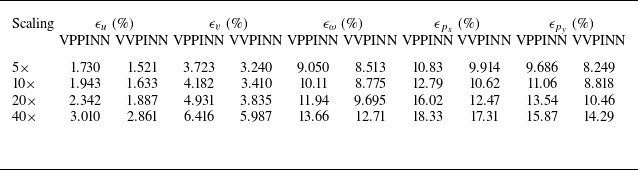
After training, both models are evaluated on the high-resolution space–time grid, and their reconstruction accuracies are summarised in table 1. For the multi-cylinder wake at
 $Re=100$
, the relative errors in the velocity components remain below
 $3.5\,\%$
for all temporal scaling factors, which is consistent with the comparatively simple dynamics of this laminar configuration. Nevertheless, systematic differences between the two formulations are evident. For all scaling factors, the VVPINN yields smaller errors in
 $\epsilon _u$
,
 $\epsilon _v$
and
 $\epsilon _\omega$
than the VPPINN, with the largest improvements observed for the vorticity, which is particularly sensitive to small-scale shear and rotation. For instance, at
 $10\times$
, the vorticity error decreases from
 $10.11\,\%$
(VPPINN) to
 $8.78\,\%$
(VVPINN), and at
 $20\times$
, from
 $11.94\,\%$
to
 $9.70\,\%$
. The velocity errors show a similar trend: at
 $20\times$
,
 $\epsilon _u$
decreases from
 $2.34\,\%$
to
 $1.89\,\%$
, and
 $\epsilon _v$
from
 $4.93\,\%$
to
 $3.84\,\%$
.
Relative
 $L_2$
errors (%) of velocity components, vorticity and pressure gradients for different temporal scaling factors in the multi-cylinder wake case.

A similar behaviour is observed for the pressure gradient errors
 $\epsilon _{p_x}$
and
 $\epsilon _{p_y}$
. For the VPPINN,
 $p_x$
and
 $p_y$
are obtained by differentiating the network-predicted pressure field, whereas for the VVPINN the pressure gradients are reconstructed a posteriori from the recovered velocity field using the planar momentum (3.11). Despite this indirect procedure, the VVPINN still delivers consistently smaller pressure gradient errors. At
 $10\times$
,
 $\epsilon _{p_x}$
decreases from
 $12.79\,\%$
to
 $10.62\,\%$
, and
 $\epsilon _{p_y}$
from
 $11.06\,\%$
to
 $8.82\,\%$
; at
 $20\times$
,
 $\epsilon _{p_x}$
decreases from
 $16.02\,\%$
to
 $12.47\,\%$
, and
 $\epsilon _{p_y}$
from
 $13.54\,\%$
to
 $10.46\,\%$
. These values indicate that the vorticity–velocity constraints lead to a more self-consistent reconstruction of both velocity gradients and pressure gradients in the multi-cylinder wake.
The temporal behaviour of the reconstruction error is shown in figure 4, which reports the time evolution of the relative
 $L_2$
errors
 $\epsilon _u(t)$
,
 $\epsilon _v(t)$
,
 $\epsilon _\omega (t)$
,
 $\epsilon _{p_x}(t)$
and
 $\epsilon _{p_y}(t)$
for the four temporal scaling factors. Solid and dashed lines denote VVPINN and VPPINN results, respectively. For all scaling factors, the VVPINN exhibits lower and smoother error levels, most notably for vorticity and the pressure gradients. As the temporal scaling factor increases from
 $5\times$
to
 $40\times$
, the errors of both models increase, reflecting the loss of temporal information in the input data. In the most extreme case of
 $40\times$
, the error curves display pronounced oscillations, with minima aligned with the available measurement instants and larger errors in between, particularly for the VPPINN. This behaviour shows that the reconstructions become increasingly tied to the sparse observation times when the sampling interval is large, whereas the vorticity–velocity formulation provides a more regularised representation and maintains a systematically lower error level under temporally sparse sampling.
Time evolution of relative
 $L_2$
errors (%) of velocity components, vorticity and pressure gradients under different temporal scaling factors in the multi-cylinder wake case. Solid lines indicate VVPINN; dashed lines indicate VPPINN.

To further illustrate the instantaneous reconstruction quality, figure 5 compares the fields
 $u$
,
 $v$
,
 $\omega$
,
 $p_x$
and
 $p_y$
predicted by the two models with the DNS reference at
 $t=12.3$
s for temporal scaling factor
 $20\times$
, together with the corresponding absolute error maps. The leftmost column shows the coarse PIV input, illustrating the loss of small-scale information that the super-resolution methods are tasked with recovering. Both methods reproduce the overall wake structure and vortex-shedding pattern. The VPPINN, however, displays noticeable smoothing and attenuation of small-scale features, particularly in the vorticity and pressure gradient fields. The VVPINN retains sharper shear layers and more distinct vortical structures, and its error fields are generally of lower amplitude and less spatially correlated, consistent with the quantitative trends in table 1 and figure 4.
Instantaneous reconstruction at
 $t=12.3$
s for temporal scaling
 $20\times$
in the multi-cylinder wake case. From left to right: coarse PIV input, VPPINN prediction, VVPINN prediction and DNS reference, followed by the absolute error fields of each formulation. Rows correspond to
 $u$
,
 $v$
,
 $\omega$
,
 $p_x$
and
 $p_y$
.

3.2. Taylor–Green vortex
To further assess the reconstruction capability in turbulent regimes, we consider the two-dimensional Taylor–Green vortex as a canonical test case. This flow evolves from an analytically prescribed initial condition into broadband, approximately homogeneous turbulence with well-defined small-scale structures (Kim & Moin Reference Kim and Moin1985). The flow is governed by the incompressible Navier–Stokes equations with periodic boundary conditions in a square domain
 $[-\pi ,\pi ]^2$
of size
 $L_x = L_y = 2\pi$
, discretised on a
 $1024\times 1024$
grid. The governing equations are
 \begin{align} \frac {\partial u}{\partial t} + u \frac {\partial u}{\partial x} + v \frac {\partial u}{\partial y} &= - \frac {1}{\rho } \frac {\partial p}{\partial x} + \nu \left ( \frac {\partial ^2 u}{\partial x^2} + \frac {\partial ^2 u}{\partial y^2} \right ) + g_x, \\[-10pt] \nonumber \end{align}
 \begin{align} \frac {\partial v}{\partial t} + u \frac {\partial v}{\partial x} + v \frac {\partial v}{\partial y} &= - \frac {1}{\rho } \frac {\partial p}{\partial y} + \nu \left ( \frac {\partial ^2 v}{\partial x^2} + \frac {\partial ^2 v}{\partial y^2} \right ) + g_y, \\[-10pt] \nonumber \end{align}
 \begin{align} \frac {\partial u}{\partial x} + \frac {\partial v}{\partial y} &= 0, \\[10pt] \nonumber \end{align}
where
 $u$
and
 $v$
are the velocity components in the
 $x$
- and
 $y$
-directions,
 $p$
is the pressure,
 $\rho$
is the density, and
 $\nu$
is the kinematic viscosity. The external forcing is prescribed as
 $g_x = 0.01 \sin 8x \cos 8y$
and
 $g_y = -0.01 \cos 8x \sin 8y$
, while
 $\nu = 4\times 10^{-4}$
and
 $\rho = 1$
, corresponding to Reynolds number
 $Re = 2500$
. The DNS are integrated over the non-dimensional time interval
 $t \in [0,60]$
. To exclude initial transient effects, 201 snapshots of the velocity fields are extracted from the statistically stationary regime (
 $t \in [20,60]$
) at sampling interval
 $\Delta t_{\textit{DNS}} = 0.2$
, and the time origin is shifted such that the analysed sequence spans
 $t \in [0,40]$
.
3.2.1. Synthetic PIV data and reconstruction set-up
To emulate planar PIV measurements, synthetic particle images are generated from the DNS velocity field on the computational plane. Randomly distributed tracer particles are seeded and advected between successive DNS snapshots. A three-level, multi-pass cross-correlation algorithm is applied, with the smallest interrogation window of
 $32\times 32$
pixels and
 $50\,\%$
overlap. This procedure yields coarse velocity fields on a
 $63\times 63$
grid, which constitute the input PIV-like measurements for the reconstruction task.
Spatial super-resolution is performed from the PIV resolution
 $63\times 63$
to the DNS resolution
 $1024\times 1024$
. Temporal super-resolution is examined at three sampling levels, denoted by scaling factors
 $5\times$
,
 $10\times$
and
 $20\times$
. Starting from the DNS sampling interval
 $\Delta t_{\textit{DNS}} = 0.2$
, coarse sequences are constructed by retaining every 5th, 10th and 20th DNS snapshot, respectively, which yields effective sampling intervals
 $\Delta t = 1$
,
 $2$
and
 $4$
. The corresponding sampling frequencies are
 $f_s = 1/\Delta t = 1.0$
,
 $0.5$
and
 $0.25$
, so that the Nyquist frequencies
 $f_{{Ny}} = f_s/2$
are
 $0.5$
,
 $0.25$
and
 $0.125$
.
The DNS sampling frequency
 $f_{s,{DNS}} = 1/\Delta t_{\textit{DNS}} = 5$
yields a DNS Nyquist frequency
 $f_{{Ny,DNS}} = 2.5$
, which is much larger than the coarsened Nyquist frequencies listed above. All sub-sampled sequences are therefore strongly temporally under-resolved relative to the DNS reference. An analogous relation holds in space. The DNS grid spacing
 $\Delta x = \Delta y = 2\pi /1024$
yields a Nyquist wavenumber
 $k_{{Ny,DNS}} = \pi /\Delta x$
that fully resolves the finest scales present in the DNS. By contrast, the coarse PIV grid of
 $63\times 63$
points has a Nyquist wavenumber
 $k_{{Ny,\textit{PIV}}}$
that is much lower than
 $k_{{Ny,DNS}}$
, so that a wide range of fine scales is filtered out. Reconstructing the flow on the
 $1024\times 1024$
grid therefore amounts to recovering wavenumbers from the under-resolved PIV measurements up to the DNS resolution, in particular across the range
 $k \gt k_{{Ny,\textit{PIV}}}$
.
3.2.2. Error metrics and pressure gradient recovery
The reconstruction accuracy is quantified using the relative
 $L_2$
error (3.1), now applied to the set of quantities
 \begin{align} O \in \{u, v, \omega , S_{12}, p_x, p_y\}, \end{align}
where
 $u$
and
 $v$
are the velocity components in the
 $x$
- and
 $y$
-directions,
 $\omega$
is the scalar vorticity,
 $S_{12}$
is the shear strain rate, and
 $p_x = \partial p / \partial x$
and
 $p_y = \partial p / \partial y$
are the pressure gradient components. The shear strain rate characterises the local deformation due to shear, and is defined as
 \begin{align} S_{12} = \frac {1}{2} \left ( \frac {\partial u}{\partial y} + \frac {\partial v}{\partial x} \right ) \!. \end{align}
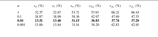
Sensitivity of VVPINN reconstruction errors to the weighting factor
 $\alpha$
for the Taylor–Green vortex at
 $10\times$
temporal super-resolution. Bold indicates the selected value.

In the VPPINN, the pressure field
 $p$
is an explicit network output, and
 $p_x$
and
 $p_y$
are obtained by automatic differentiation. In the VVPINN, the pressure is eliminated from the training loss; the pressure gradients are instead recovered a posteriori from the reconstructed velocity field by rearranging the non-dimensional form of the forced momentum equations (3.7). In non-dimensional variables with
 $\rho =1$
and
 $\nu = 1/Re$
, these equations are
 \begin{align} \frac {\partial u}{\partial t} + u \frac {\partial u}{\partial x} + v \frac {\partial u}{\partial y} &= - p_x + \frac {1}{Re} \left ( \frac {\partial ^2 u}{\partial x^2} + \frac {\partial ^2 u}{\partial y^2} \right ) + g_x, \\[-10pt] \nonumber \end{align}
 \begin{align} \frac {\partial v}{\partial t} + u \frac {\partial v}{\partial x} + v \frac {\partial v}{\partial y} &= - p_y + \frac {1}{Re} \left ( \frac {\partial ^2 v}{\partial x^2} + \frac {\partial ^2 v}{\partial y^2} \right ) + g_y. \\[10pt] \nonumber \end{align}
Solving for the pressure gradients yields
 \begin{align} p_x &= - \biggl [ \frac {\partial u}{\partial t} + u \frac {\partial u}{\partial x} + v \frac {\partial u}{\partial y} - \frac {1}{Re} \left ( \frac {\partial ^2 u}{\partial x^2} +\frac {\partial ^2 u}{\partial y^2} \right ) - g_x \biggr ], \\[-10pt] \nonumber \end{align}
 \begin{align} p_y &= - \biggl [ \frac {\partial v}{\partial t} + u \frac {\partial v}{\partial x} + v \frac {\partial v}{\partial y} - \frac {1}{Re} \left ( \frac {\partial ^2 v}{\partial x^2} +\frac {\partial ^2 v}{\partial y^2} \right ) - g_y \biggr ], \\[10pt] \nonumber \end{align}
which are evaluated using the VVPINN-predicted velocity field and its derivatives.
3.2.3. Training settings
The construction of training data (coarse PIV measurements plus collocation points on the high-resolution space–time mesh) and the mixed mini-batch sampling strategy are identical to those in the multi-cylinder wake case: each mini-batch contains
 $N_b = 15\,360$
samples with measurement fraction
 $\chi _{{meas}} = 0.20$
, and collocation points are generated by Latin hypercube sampling. Both VPPINNs and VVPINNs employ the same network architecture as in the previous case (one input layer, eight hidden layers with 512 neurons each, and one output layer with
 $\tanh$
activation). The physics-informed loss uses the same data and equation terms (2.9)–(2.14), but with a reduced weight
 $\alpha = 0.01$
to account for the stronger small-scale activity of Taylor–Green turbulence. The guiding principle for selecting
 $\alpha$
is to balance the magnitudes of
 $L_{\textit{data}}$
and
 $\alpha L_{\textit{eqns}}$
during the initial phase of training. In the multi-cylinder wake case,
 $\alpha = 1$
suffices because the flow is dominated by large-scale vortex shedding, and the two loss components remain of similar order; here, the broadband multi-scale dynamics produces equation residuals that are orders of magnitude larger than the data loss, necessitating a reduced weight. Table 2 summarises the sensitivity of the VVPINN reconstruction errors to
 $\alpha$
for the
 $10\times$
case: values that are too large (
 $\alpha = 1$
) prevent adequate data fitting, while values that are too small (
 $\alpha = 0.001$
) weaken the physics regularisation and increase errors in derived quantities such as pressure gradients. The value
 $\alpha = 0.01$
yields the best overall trade-off and is adopted herein. The optimisation is carried out for
 $N_{{it}} = 52\,000$
iterations using the Adam optimiser with base learning rate
 $\ell _0 = 10^{-3}$
, following the same cosine warm-up and decay schedule as in the multi-cylinder wake case.
3.2.4. Training behaviour
We first examine how the vorticity reconstruction evolves during training. Figure 6 shows the predicted vorticity fields
 $\omega _{\textit{VPPINN}}$
and
 $\omega _{\textit{VVPINN}}$
at
 $t=10.6$
for temporal scaling factor
 $10\times$
, which represents one of the most challenging cases considered. Both models start from smooth, large-scale fields, and progressively develop small-scale vortical structures as optimisation proceeds. The VVPINN recovers fine-scale features earlier and more clearly than the VPPINN, whose vorticity field remains overly smooth at intermediate iterations, indicating slower convergence towards the turbulent attractor.
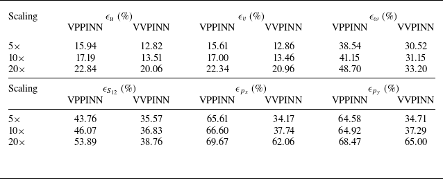
Relative
 $L_2$
errors (%) of velocity components, vorticity, shear strain rate and pressure gradients for different temporal super-resolution factors in the Taylor–Green vortex case.

Evolution of reconstructed vorticity fields
 $\omega$
at
 $t=10.6$
during training for temporal scaling factor
 $10\times$
in the Taylor–Green vortex case: (a) VPPINN, (b) VVPINN. Columns correspond to different optimisation iterations as indicated.

3.2.5. Global error statistics
After training, the two models are evaluated on the
 $1024\times 1024$
space–time grid, and the relative
 $L_2$
errors are summarised in table 3. Because the Taylor–Green turbulence contains a broad range of active scales, the reconstruction errors are larger than in the multi-cylinder wake. The VVPINN consistently outperforms the VPPINN across all temporal scaling factors and all quantities. For the velocity components, the errors lie between
 $13\,\%$
and
 $23\,\%$
; at
 $5\times$
and
 $10\times$
, the VVPINN reduces
 $\epsilon _u$
from
 $15.9$
–
 $17.2\,\%$
to
 $12.8$
–
 $13.5\,\%$
, and
 $\epsilon _v$
from
 $15.6$
–
 $17.0\,\%$
to
 $12.9$
–
 $13.5\,\%$
, whereas at
 $20\times$
, both models deteriorate, and the improvement becomes more modest. The gains are more pronounced for vorticity and shear strain rate:
 $\epsilon _\omega$
decreases from
 $38.5\,\%$
,
 $41.2\,\%$
and
 $48.7\,\%$
to
 $30.5\,\%$
,
 $31.2\,\%$
and
 $33.2\,\%$
, and
 $\epsilon _{S_{12}}$
from
 $43.8\,\%$
,
 $46.1\,\%$
and
 $53.9\,\%$
to
 $35.6\,\%$
,
 $36.8\,\%$
and
 $38.8\,\%$
at
 $5\times$
,
 $10\times$
and
 $20\times$
, respectively, corresponding to reductions of approximately
 $8$
–
 $16$
percentage points. For the pressure gradients, the VPPINN errors range from
 $65.6\,\%$
to
 $69.7\,\%$
for
 $p_x$
, and from
 $64.6\,\%$
to
 $68.5\,\%$
for
 $p_y$
, while the VVPINN lowers these values to
 $34.2$
–
 $37.3\,\%$
at
 $5\times$
and
 $10\times$
(a reduction of approximately
 $30$
percentage points), but only to
 $62.1\,\%$
and
 $65.0\,\%$
at
 $20\times$
, where the strong temporal under-sampling limits the achievable improvement. Thus although the vorticity–velocity formulation yields systematic improvements at all scaling levels, the most aggressive super-resolution factor (
 $20\times$
) remains strongly under-resolved and is associated with higher, more oscillatory error levels discussed below.
3.2.6. Temporal error evolution
Figure 7 shows the temporal evolution of the relative
 $L_2$
errors for all quantities and temporal scaling factors. For every quantity and scaling factor, the VVPINN (solid lines) exhibits lower and smoother errors than the VPPINN (dashed lines), with the most pronounced differences in
 $\omega$
,
 $S_{12}$
and the pressure gradients. As the scaling factor increases from
 $5\times$
to
 $20\times$
, the errors of both models increase, reflecting the stronger temporal under-sampling, but the growth is systematically weaker for the VVPINN. At the moderate scaling factors (
 $5\times$
and
 $10\times$
), the VPPINN curves display sharp intermittent spikes, whereas the VVPINN errors vary more smoothly in time, indicating greater robustness. For the most strongly under-sampled case (
 $20\times$
), the error histories develop pronounced oscillations, with local minima close to the measurement instants, and significantly larger errors in between, again with consistently lower levels for the vorticity–velocity formulation.
Temporal evolution of relative
 $L_2$
errors (%) of velocity components, vorticity, shear strain rate and pressure gradients under different temporal scaling factors in the Taylor–Green vortex case. Solid lines indicate VVPINN; dashed lines indicate VPPINN.

3.2.7. Instantaneous fields
Figure 8 shows instantaneous fields of
 $u$
,
 $v$
,
 $\omega$
,
 $S_{12}$
,
 $p_x$
and
 $p_y$
at
 $t=10.6$
for temporal scaling factor
 $10\times$
, together with the DNS reference and the corresponding absolute error maps. The coarse PIV input (leftmost column) highlights the substantial loss of fine-scale structures at this resolution, against which the improvement achieved by the reconstructions can be directly assessed. Additional snapshots at other times and for temporal super-resolution factors
 $5\times$
,
 $10\times$
and
 $20\times$
are provided in supplementary movies 1, 2 and 3 are available at https://doi.org/10.1017/jfm.2026.11469. Both models reproduce the large-scale velocity patterns reasonably well, and the reconstructed
 $u$
and
 $v$
fields closely match the DNS. By contrast, the vorticity and shear fields exhibit more pronounced differences: the VPPINN displays irregular, noisy structures, with spurious small-scale patches (indicated by dashed circles) that have no counterpart in the DNS, indicating a lack of physical consistency in the velocity gradients under the velocity–pressure formulation.
Instantaneous reconstructed fields at
 $t=10.6$
for temporal scaling factor
 $10\times$
in the Taylor–Green vortex case. From left to right: coarse PIV input, VPPINN prediction, VVPINN prediction and DNS reference, followed by the absolute error fields of each formulation. Rows correspond to
 $u$
,
 $v$
,
 $\omega$
,
 $S_{12}$
,
 $p_x$
and
 $p_y$
.

For the pressure gradients
 $p_x$
and
 $p_y$
, both reconstructions capture the overall sign distribution, but they differ markedly in their small-scale organisation. The VPPINN fields are comparatively diffuse, and miss many of the filamentary structures and localised extrema visible in the DNS, which is reflected in broad patches of elevated error in the corresponding difference maps. By contrast, the VVPINN recovers a much richer set of fine-scale
 $p_x$
and
 $p_y$
structures in closer visual agreement with the DNS, and the associated absolute error fields are more fragmented and of generally smaller amplitude.
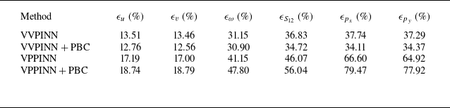
Although the periodic boundary conditions of the Taylor–Green vortex can be explicitly enforced as an additional loss term to further reduce boundary errors (see Appendix A), most practical PIV experiments do not provide such periodicity information. Therefore, the main results presented in this work are obtained without imposing periodic boundary conditions, and the relative advantage of the VVPINN over the VPPINN is preserved in both settings.
3.2.8. Spectral behaviour
Figure 9 compares the spectra of the reconstructed fields with those of the DNS. Figure 9(a) shows the turbulent kinetic energy spectrum
 $E(k)$
as a function of wavenumber
 $k$
, obtained by averaging over all DNS snapshots in time. Figure 9(b) presents the temporal energy spectrum
 $E(f)$
as a function of frequency
 $f$
, computed by averaging over all spatial locations. The vertical dashed lines indicate the Nyquist wavenumber
 $k_{{Ny}}$
and Nyquist frequency
 $f_{{Ny}}$
associated with the PIV sampling.
Spectral comparison between DNS (solid black), VPPINN (dashed blue) and VVPINN (dash-dotted red) for the Taylor–Green vortex case: (a) turbulent kinetic energy spectrum
 $E(k)$
; (b) temporal energy spectrum
 $E(f)$
. Vertical dashed lines indicate the Nyquist wavenumber
 $k_{{Ny}}$
and Nyquist frequency
 $f_{{Ny}}$
.

Both reconstructions follow the DNS spectra closely at large scales, but differences emerge at higher wavenumbers. As
 $k$
approaches and exceeds the Nyquist wavenumber
 $k_{{Ny}}$
, the spectral discrepancies increase. The VPPINN tends to overestimate the energy content beyond
 $k_{{Ny}}$
, leading to larger errors in the high-wavenumber range. The VVPINN, by contrast, preserves the spectral slope and magnitude more accurately well beyond
 $k_{{Ny}}$
. Both reconstructions yield temporal spectra
 $E(f)$
that agree well with the DNS well beyond the Nyquist frequency
 $f_{{Ny}}$
, demonstrating effective temporal super-resolution.
This apparent asymmetry between frequency and wavenumber space is consistent with how information enters the reconstruction problem. In the present set-up, the training data provide strong constraints on the time history at each sampled location, whereas the smallest spatial scales are never directly observed because the interrogation grid is much coarser than the DNS grid spacing, and wavenumbers beyond
 $k_{{Ny}}$
are entirely inferred rather than measured. Coupled with the Navier–Stokes dynamics, these temporal constraints are sufficient to recover the evolution of the energy-containing structures and their high-frequency signatures at fixed locations, but they do not uniquely determine the detailed spatial arrangement of sub-grid vortices and shear layers. Moreover, the PINN loss and network parametrisation favour smooth fields, so that the reconstructions reproduce the measured temporal signals while distributing kinetic energy over comparatively low wavenumbers, and under-populating the high-
 $k$
tail. From a physical point of view, the temporal spectrum at a fixed location is dominated by the sweeping of large-scale coherent structures, so modest smearing or displacement of fine-scale vortices has only a limited impact on
 $E(f)$
. By contrast, the wavenumber spectra are extremely sensitive to such small spatial misalignments: even slight broadening or diffusion of the smallest scales tends to redistribute energy towards lower wavenumbers, and under-populate the high-
 $k$
tail. As a result, the temporal spectrum
 $E(f)$
is recovered very accurately, whereas the wavenumber spectra remain more susceptible to discrepancies in the representation of fine-scale structures.
Taken together, these observations confirm that the vorticity–velocity formulation provides a more faithful and physically consistent representation of the small-scale dynamics than the velocity–pressure formulation in the Taylor–Green vortex case, while also highlighting that temporal super-resolution is intrinsically better conditioned than the recovery of high-wavenumber spatial content from strongly under-resolved planar data.
3.3. An experimental case of flow past two cylinders of different sizes
The proposed method is further validated using an experimental case of flow past two side-by-side circular cylinders of different diameters (the smaller cylinder diameter is
 $D = 8$
mm), conducted in a recirculating open water channel with cross-section
 $150\times 250$
mm
 $^2$
(see Liu et al. (Reference Liu, Shi and Yu2011) for facility details). We note that PIV data from this platform were successfully employed in the pioneering work of Deng et al. (Reference Deng, He, Liu and Kim2019), who demonstrated the impressive capability of ESRGAN to recover high-fidelity spatial structures in turbulent velocity fields. A spacing ratio
 $G/D = 2.0$
was tested to investigate the wake interaction between the cylinders. The free-stream velocity was maintained at
 $U_0 = 0.125$
m s
 $^{-1}$
, corresponding to Reynolds number
 $Re_D = U_0 D/\nu \approx 1000$
based on the smaller cylinder diameter. The turbulence intensity of the incoming flow was less than
 $2\,\%$
. The water channel walls were made of Plexiglas to ensure optical access for planar PIV measurements.
The mid-plane of the flow field was illuminated by an 8 W continuous wave laser (wavelength
 $532$
nm, sheet thickness
 $\approx 1$
mm), and the flow was seeded with glass particles (
 $\rho _p \approx 1.05$
kg m
 $^{-3}$
,
 $d_p \approx 10$
 $\unicode{x03BC}$
m). The measurement region spanned
 $7.2D\times 7.2D$
downstream of the cylinders, as illustrated in figure 10. A high-speed CMOS camera (Mikrotron,
 $1024\times 1024$
px) was operated at framing rate 250 Hz. After multi-pass cross-correlation with minimum interrogation window
 $32\times 32$
px and
 $50\,\%$
overlap, the PIV processing yielded
 $63\times 63$
velocity vectors, corresponding to physical spacing
 $0.9\times 0.9$
mm
 $^2$
. Using
 $U_0$
and
 $D$
to render velocity and length dimensionless, the measurement domain becomes
 $[0,7.2]\times [0,7.2]$
. From the full PIV sequence, 201 snapshots were extracted, with non-dimensional time step
 $\Delta t = 0.125$
, spanning a total interval
 $t \in [0,25]$
in convective units (
 $U_0 t/D$
), providing a high time resolution reference sequence that resolves the unsteady wake dynamics.
Schematic of the experimental set-up for the wake behind two side-by-side circular cylinders of different diameters. The shaded region indicates the PIV measurement window, covering
 $7.2D\times 7.2D$
in the downstream wake of the cylinders.

Spatial super-resolution is performed from the PIV resolution
 $63\times 63$
to a reconstruction grid
 $1024\times 1024$
. Temporal super-resolution is examined at four sampling levels, obtained by retaining every 4th, 8th, 16th and 32nd snapshot of the reference sequence. These correspond to effective time steps
 $\Delta t^* = 0.5$
,
 $1.0$
,
 $2.0$
and
 $4.0$
, so that the flow is advanced by approximately
 $0.5D$
,
 $1D$
,
 $2D$
and
 $4D$
, respectively, between two consecutive measurements. The coarsened PIV sequences therefore represent strongly under-resolved observations in time, especially at the largest interval.
3.3.1. Instantaneous fields
We first examine the instantaneous reconstruction quality for representative temporal super-resolution factor
 $8\times$
. Additional snapshots and results for temporal super-resolution factors
 $4\times$
,
 $8\times$
,
 $16\times$
and
 $32\times$
are provided in supplementary movies 4, 5, 6 and 7. Figure 11 shows the reconstructed fields of
 $u$
,
 $v$
,
 $\omega$
,
 $S_{12}$
,
 $p_x$
and
 $p_y$
at
 $t=4.125$
, together with the corresponding raw PIV fields. Both reconstructions reproduce the large-scale wake structure and the main shear-layer undulations, whereas the PIV data exhibit pronounced small-scale noise. The VPPINN yields reasonably smooth velocity components, but its vorticity and shear-strain fields still contain fragmented patches and short filaments that are difficult to associate with coherent flow features. In contrast, the VVPINN recovers well-defined vortex cores and continuous shear layers, with structures that are more clearly organised along the separated shear layers and in the near-wake region.
For the pressure gradients, the fields obtained directly from the PIV measurements are dominated by pixel-scale fluctuations, and lack coherent large-scale organisation. Both reconstructions strongly suppress this measurement noise, and produce smoother
 $p_x$
and
 $p_y$
distributions. The VPPINN, however, tends to generate relatively diffuse extrema, and misses part of the organised pattern associated with the shear layers, whereas the VVPINN produces more localised positive- and negative-gradient lobes that are aligned with the vortical and shear structures seen in
 $\omega$
and
 $S_{12}$
. Overall, the VVPINN fields exhibit a clearer separation between the wake region and the outer flow, and provide a more physically plausible picture of the instantaneous vorticity, shear and pressure gradient distributions than either the VPPINN or the PIV-derived quantities.
Instantaneous reconstructed fields at
 $t=4.125$
for temporal scaling factor
 $8\times$
in the two-cylinder experiment. From left to right: VPPINN reconstruction, VVPINN reconstruction and PIV field. Rows correspond to
 $u$
,
 $v$
,
 $\omega$
,
 $S_{12}$
,
 $p_x$
and
 $p_y$
, respectively.

3.3.2. Root mean square statistics
To assess how well the unsteady wake dynamics are reproduced, we compute root mean square (RMS) fluctuations of the reconstructed velocity and gradient fields,
 \begin{align} u'_{\textit{rms}}(x,y) & = \sqrt {\frac {1}{T}\int _0^T \bigl [u(x,y,t)-\overline {u}(x,y)\bigr ]^2\,\mathrm{d}t}, \nonumber \\[4pt] v'_{\textit{rms}}(x,y) & = \sqrt {\frac {1}{T}\int _0^T \bigl [v(x,y,t)-\overline {v}(x,y)\bigr ]^2\,\mathrm{d}t}, \end{align}
with analogous definitions for
 $\omega '_{\textit{rms}}$
and
 $S'_{12,{rms}}$
, where
 $\overline {({\cdot })}$
denotes temporal averaging over the sampling interval
 $T$
.
Comparison of reconstructed RMS fields for temporal scaling factor
 $8\times$
in the two-cylinder experiment. From left to right: VPPINN, VVPINN and PIV reference. Rows correspond to
 $u'_{\textit{rms}}$
,
 $v'_{\textit{rms}}$
,
 $\omega '_{\textit{rms}}$
and
 $S'_{12,{rms}}$
, respectively.

Figure 12 compares the RMS distributions of
 $u'_{\textit{rms}}$
,
 $v'_{\textit{rms}}$
,
 $\omega '_{\textit{rms}}$
and
 $S'_{12,{rms}}$
for temporal scaling factor
 $8\times$
. For the velocity components, both reconstructions correctly identify the main regions of enhanced fluctuations in the upper and lower shear layers and in the near-wake recirculation zone, and the amplitude levels are close to those inferred from the PIV data, but without the small-scale speckle noise that contaminates the raw measurements. The VPPINN fields are somewhat more diffuse, whereas the VVPINN preserves sharper
 $u'_{\textit{rms}}$
and
 $v'_{\textit{rms}}$
bands along the shear layers.
Differences between the two formulations are more evident in the gradient statistics. For
 $\omega '_{\textit{rms}}$
and
 $S'_{12,{rms}}$
, the PIV-derived fields show a noisy background on which the dominant shear-layer peaks are superimposed. Both reconstructions suppress much of this small-scale noise, but the VPPINN tends to produce elongated streaks and locally overdamped regions that only loosely follow the shear layers. By contrast, the VVPINN yields more continuous high-intensity bands that are better aligned with the vortical and shear structures seen in the mean wake. Overall, the RMS statistics confirm that the vorticity–velocity formulation provides a more physically plausible and better organised representation of the fluctuating vorticity and shear than the velocity–pressure formulation.
4. Conclusions
We have investigated the reconstruction of high-resolution unsteady flow fields from low space–time resolution planar PIV data using physics-informed neural networks (PINNs). The focus has been on how the choice of governing-equation formulation affects the ability of PINNs to recover small-scale structures, shear and pressure gradients from sparse and noisy measurements. To this end, two architectures with identical network structure, normalisation and training strategy were compared: a conventional velocity–pressure PINN (VPPINN) and a vorticity–velocity PINN (VVPINN), which differ only in the physical constraints enforced in the loss function.
First, in terms of global error measures, the vorticity–velocity formulation systematically outperforms the velocity–pressure formulation in all three test cases. In the laminar multi-cylinder wake, the VVPINN yields slightly smaller
 $L_2$
errors in the velocity components and vorticity, together with consistently lower pressure gradient errors for all temporal scaling factors. In the two-dimensional Taylor–Green vortex, where broadband multi-scale dynamics and intense small-scale activity make the reconstruction more demanding, the advantage of the vorticity–velocity formulation becomes more pronounced: over the range
 $5\times$
–
 $20\times$
temporal super-resolution, the VVPINN reduces the
 $L_2$
errors in the velocity components by a few percentage points, and in vorticity and shear strain rate by approximately
 $10\,\%$
, while the pressure gradient errors are lowered by up to approximately
 $30\,\%$
at the moderate factors (
 $5\times$
and
 $10\times$
).
Second, the instantaneous fields and derived gradient quantities obtained from the VVPINN are more consistent with the underlying flow physics than those from the VPPINN. In the Taylor–Green vortex, the VPPINN produces highly irregular and noisy patterns in vorticity and shear that lack clear correspondence with the DNS structures, as well as comparatively diffuse and biased pressure gradient fields. The VVPINN, by contrast, recovers coherent small-scale vortices and shear layers that align well with the reference fields, and yields finer, more organised
 $p_x$
and
 $p_y$
structures. In the experimental wake of two side-by-side cylinders, both PINNs suppress part of the measurement noise present in the raw PIV data, but the VVPINN provides smoother velocity fields, more coherent vorticity and shear distributions, and pressure gradients that are less contaminated by small-scale speckle and more consistent with the large-scale wake organisation. The RMS statistics corroborate these findings, showing that the vorticity–velocity formulation gives a more physically plausible and better organised representation of the fluctuating vorticity and shear.
Third, the spectral analysis reveals a clear contrast between the recovery of frequency and wavenumber content. In the Taylor–Green vortex case, both formulations reproduce the temporal energy spectrum
 $E(f)$
accurately over a wide frequency range, including frequencies well beyond the Nyquist frequency
 $f_{{Ny}}$
, confirming that the physics-informed reconstruction successfully breaks through the temporal Nyquist limit. By contrast, neither model fully recovers the highest wavenumbers in the turbulent kinetic energy spectrum: even with the VVPINN, the reconstructed spectra deviate from the DNS for wavenumbers beyond the Nyquist limit of the sampled PIV data, and tend to under-populate the high-
 $k$
range. This behaviour reflects the way information enters the reconstruction problem: the training data strongly constrain the temporal histories at the sampled locations, whereas the smallest spatial scales are only indirectly informed by the combination of coarse PIV resolution and pointwise partial differential equation residuals. As a result, temporal super-resolution is better conditioned than the recovery of high-wavenumber spatial content from strongly under-resolved planar PIV data.
Overall, the present results demonstrate that vorticity-based constraints provide a more effective route to physics-consistent super-resolution of sub-sampled PIV data than the conventional velocity–pressure formulation, especially for quantities involving velocity gradients. All test cases considered here are two-dimensional, reflecting the focus on planar PIV – the most widely used velocity measurement configuration in experimental fluid mechanics. The VVPINN formulation can in principle be extended to three-dimensional flows by incorporating the full vorticity transport equation, including the vortex stretching term
 $(\boldsymbol{\omega }\boldsymbol{\cdot }\boldsymbol{\nabla })\boldsymbol{u}$
, although practical challenges related to the increased computational cost of four-dimensional inputs, the higher-order derivatives introduced by the stretching term, and the sparsity of volumetric experimental data remain to be addressed. Future work will therefore explore the extension to three-dimensional turbulent flows, application to more challenging strongly unsteady configurations such as sweeping jets or flows with large-scale separation, the incorporation of explicit spectral information into the PINN framework, e.g. via Fourier-feature embeddings or multi-resolution spectral losses, and the use of irregularly sampled particle tracking velocimetry measurements to compute wavenumber spectra without resorting to fast Fourier transforms on coarse interrogation grids, with the aim of further improving the reconstruction of fine-scale flow structures from sparse experimental data.
Supplementary movies
Supplementary movies are available at https://doi.org/10.1017/jfm.2026.11469.
Acknowledgements
The authors gratefully acknowledge Professor Y. Chen (Eastern Institute of Technology, Ningbo, China) and Professor C. Lin (Fudan University, Shanghai, China) for kindly providing the Taylor–Green vortex DNS dataset used in § 3.2. C.T. also gratefully acknowledges support from the international exchange programme ‘Carbon neutral power technology and systems’, funded by the State Administration of Foreign Experts Affairs (SAFEA) of China.
Funding
This work was supported by the National Natural Science Foundation of China (grant nos. U25B2088, 12572382 and 12521002) and the Shanghai Municipal Science and Technology Commission (grant no. 25ZR1401194).
Declaration of interests
The authors report no conflict of interest.
Appendix A. Effect of periodic boundary conditions
The main results for the Taylor–Green vortex presented in § 3.2 are obtained without imposing explicit boundary constraints, since such exact global spatial information is generally unavailable in practical PIV measurements. However, the theoretical Taylor–Green vortex is spatially periodic on the domain
 $[-\pi ,\pi ]^{2}$
, and this prior knowledge can in principle be exploited to regularise the reconstruction near the domain edges. In this appendix, we systematically compare the performance of both the VVPINN and VPPINN formulations with and without periodic boundary conditions (PBC).
A.1. Implementation of PBC
The periodic constraint is explicitly enforced during training by augmenting the total loss function with a boundary penalty term
 $\mathcal{L}_{{PBC}} = \mathcal{L}_{\textit{PBC},x} + \mathcal{L}_{{PBC},y}$
, defined as
 \begin{align} \begin{aligned} \mathcal{L}_{\textit{PBC},x} &= \frac {1}{N_{bc}}\sum _{i=1}^{N_{bc}} \left \lVert \boldsymbol{u}(-\pi , y_i, t_i) - \boldsymbol{u}(\pi , y_i, t_i) \right \rVert _{2}^{2}, \\[4pt] \mathcal{L}_{{PBC},y} &= \frac {1}{N_{bc}}\sum _{i=1}^{N_{bc}} \left \lVert \boldsymbol{u}(x_i, -\pi , t_i) - \boldsymbol{u}(x_i, \pi , t_i) \right \rVert _{2}^{2}, \end{aligned} \end{align}
where
 $N_{bc}$
is the number of collocation pairs randomly sampled on opposite boundaries at each iteration (set to
 $N_{bc}=1024$
in this study).
For both the baseline VPPINN and the proposed VVPINN, the periodic constraint is applied identically to the primary velocity components, i.e.
 $\boldsymbol{u} = (u, v)^{{\rm T}}$
. The total loss is then given by
 $\mathcal{L}_{\textit{total}} = \mathcal{L}_{\textit{data}} + \alpha \mathcal{L}_{\textit{eqns}} + \beta \mathcal{L}_{{PBC}}$
, where
 $\beta =1.0$
is the weighting factor for the boundary conditions.
A.2. Performance comparison
Table 4 compares the global reconstruction errors for both PINN methods with and without the inclusion of
 $\mathcal{L}_{{PBC}}$
.
Relative
 $L_2$
errors (%) of velocity components, vorticity, shear strain rate and pressure gradients for the VVPINN and the VPPINN, with and without PBC, in the Taylor–Green vortex case at
 $10\times$
temporal super-resolution. The VVPINN benefits from the additional constraint, whereas the VPPINN accuracy degrades due to the unconstrained pressure boundaries, causing optimisation conflicts.

For the VVPINN, imposing periodicity yields a modest but highly consistent improvement across all physical quantities. The velocity errors decrease by approximately
 $0.8$
percentage points, shear strain rate errors by
 $2.1$
percentage points, and pressure gradient errors by
 $3$
–
 $3.6$
percentage points. Because the VVPINN completely eliminates pressure from the governing equations, enforcing periodic boundaries solely on the velocity field is physically sufficient and highly compatible with the vorticity transport mechanism, allowing the network to natively benefit from the additional boundary regularisation.
By contrast, the VPPINN exhibits a significant degradation in accuracy when the identical PBC are added. Velocity errors increase by over
 $1.5$
percentage points, and the pressure gradient errors rise sharply from approximately
 $65\,\%$
to nearly
 $79\,\%$
. This counter-intuitive behaviour is rooted in the mathematical structure of the formulations. In the VPPINN, the momentum equations tightly couple velocity and pressure. When periodic constraints are imposed solely on the velocity field (
 $\boldsymbol{q} = (u, v)^{{\rm T}}$
), the implicit pressure field remains unconstrained at the boundaries. The network therefore struggles to reconcile the forced velocity boundary conditions with the unregularised pressure gradients within the Navier–Stokes residuals. This mismatch introduces conflicting gradient signals (stiffness) during back propagation, which ultimately destabilises the training dynamics and exacerbates the errors in derivative quantities.
Figure 13 visualises the absolute vorticity error fields for all four configurations. Comparing the top row (VPPINN) with the bottom row (VVPINN) confirms that the VVPINN produces consistently lower error magnitudes regardless of whether periodicity is enforced. Furthermore, the VPPINN + PBC field (top right) shows notably increased error concentrations relative to the baseline VPPINN (top left), corroborating the quantitative trends in table 4. Conversely, for the VVPINN (bottom row), the periodic constraint leads to a visible reduction of errors near the physical boundaries, reflecting the numerical improvements reported above.
Absolute vorticity error fields
 $|\omega _{{ref}}-\omega |$
for the Taylor–Green vortex reconstruction at
 $t = 10.6$
. Top row: VPPINN without (left) and with (right) PBC. Bottom row: VVPINN without (left) and with (right) PBC. The VVPINN maintains robust performance and lower errors in both settings, while the VPPINN shows increased errors and structural deterioration when periodicity is imposed.

These results reinforce two central conclusions. First, the VVPINN robustly outperforms the VPPINN with or without exact PBC, confirming that the advantage of the vorticity–velocity formulation is inherent and not contingent on specific boundary information. Second, imposing partial boundary constraints (e.g. on velocity but not pressure) into PINNs does not unconditionally guarantee improved accuracy; the VPPINN’s strong-form residual is evidently less resilient to the resulting unconstrained boundary derivatives. Because exact and complete PBC are rarely available in realistic experimental configurations, the primary analysis in this paper appropriately employs the unconstrained formulation (
 $\beta =0$
).