



1. Introduction
Acoustic cavitation has been an active area of research since the early twentieth century. In this phenomenon, bubbles – typically in the micron-size range at the lower end – are placed inside a liquid domain and excited by high-frequency ultrasound (Neppiras Reference Neppiras1980; Leighton Reference Leighton2012). The developed periodic pressure field drives the bubbles through cycles of expansion followed by violent collapse (Suslick et al. Reference Suslick, Didenko, Fang, Hyeon, Kolbeck, McNamara, Mdleleni and Wong1999; Mettin Reference Mettin2005; Mettin Reference Mettin2007). Under certain conditions, the bubble-wall velocity during collapse can approach the speed of sound in the liquid, producing extreme local conditions (Flint & Suslick Reference Flint and Suslick1991; Suslick & Flannigan Reference Suslick and Flannigan2008) that motivate continued scientific interest. When the collapse is sufficiently intense, temperatures of the order of 8000 K and pressures approaching 1000 bar have been reported inside the bubble (Brennen Reference Brennen1995), accompanied by the emission of strong shock waves into the surrounding liquid (Birkin et al. Reference Birkin, Offin, Joseph and Leighton2005; Yasui Reference Yasui2017; Khavari et al. Reference Khavari, Priyadarshi, Morton, Porfyrakis, Pericleous, Eskin and Tzanakis2023). Potential applications of acoustic cavitation are diverse and can broadly be classified into two categories: those that aim to exploit the extreme conditions generated within the bubble, and those that seek to utilise the intense shock waves transmitted into the liquid. The elevated pressures and temperatures inside collapsing bubbles have been investigated as a means to drive chemical reactions, including the synthesis of ammonia (Kubicsek et al. Reference Kubicsek, Kozák, Turányi, Zsély, Papp, Al-Awamleh and Hegedûs2024; Kubicsek & Hegedűs Reference Kubicsek and Hegedűs2025; Kubicsek et al. Reference Kubicsek, Hegedűs and Csizmadia2025), hydrogen (Hegedűs et al. Reference Hegedűs, Kalmár, Turányi, Zsély and Papp2022; Kalmár et al. Reference Kalmár, Turányi, Zsély, Papp and Hegedűs2022) and reactive radicals (e.g. H
 $\bullet$
) (Merouani et al. Reference Merouani, Hamdaoui, Rezgui and Guemini2015), the formation of nanoparticles (Kwan et al. Reference Kwan, Graham, Myers, Carlisle, Stride and Coussios2015; Kumar et al. Reference Kumar, Singh and Garg2019a
,
Reference Kumar, Singh and Gargb
) and the degradation of anionic surfactants in wastewater treatment (Yi et al. Reference Yi, Lu, Wang, Wang and Yang2018). The shock waves emitted into the surrounding liquid are being explored in biomedical contexts, such as lithotripsy for kidney stone fragmentation (Bailey et al. Reference Bailey, Crum, Sapozhnikov, Evan, McAteer, Colonius and Cleveland2003; Ikeda et al. Reference Ikeda, Yoshizawa, Tosaki, Allen, Takagi, Ohta, Kitamura and Matsumoto2006; Ikeda et al. Reference Ikeda, Yoshizawa, Koizumi, Mitsuishi and Matsumoto2016), histotripsy for ablation of tumours and blood clots (Yeats et al. Reference Yeats, Lu, Sukovich, Xu and Hall2023) and the enhancement of drug delivery across cell membranes (Coussios & Roy Reference Coussios and Roy2008; Ueda et al. Reference Ueda, Mutoh, Seki, Kobayashi and Morimoto2009). In materials science, ongoing research considers the use of cavitation-induced shock waves for surface cleaning (Potter et al. Reference Potter, Tokranova, Rastegar and Castracane2016; Verhaagen & Rivas Reference Verhaagen and Rivas2016), peening (Soyama Reference Soyama2024; Siva Rao et al. Reference Siva Rao, Chakladar and Paul2025), hardening (Shchukin et al. Reference Shchukin, Skorb, Belova and Möhwald2011; Tsvetkov et al. Reference Tsvetkov, Gorbachenko and Fiaktistov2019) and modification.
From an application standpoint, larger bubbles are generally considered advantageous as they can accommodate greater quantities of chemicals and displace larger liquid volumes, thereby generating stronger shock waves. However, as the bubble radius increases, surface tension becomes insufficient to maintain sphericity (Mettin Reference Mettin2005, Reference Mettin2007). The resulting non-spherical oscillations reduce energy focusing, weaken compression and may ultimately cause bubble fragmentation (Brennen Reference Brennen1995; Dollet et al. Reference Dollet, van der Meer, Garbin, de Jong, Lohse and Versluis2008; Holzfuss Reference Holzfuss2008). Thus, sustaining large bubbles that oscillate in a spherical or nearly spherical manner is a fundamental requirement for many prospective applications. Conversely, some applications intentionally exploit stable non-spherical oscillations, as these promote efficient microstreaming in the surrounding liquid – a phenomenon leveraged for cell (Ahmed et al. Reference Ahmed, Ozcelik, Bojanala, Nama, Upadhyay, Chen, Hanna-Rose and Huang2016) and microparticle (Peng et al. Reference Peng, Zhou, Yuan and Jiang2021) manipulation, as well as biochemical analysis (Gogate & Kabadi Reference Gogate and Kabadi2009). Therefore, accurate numerical models capable of capturing non-spherical bubbly dynamics, validated by experimental measurements, are essential for the design and optimisation of these applications.
Experimental investigations of non-spherical bubble dynamics are rare in the literature due to the inherent challenges of observing micron-scale phenomena on a microsecond time scale. One of the most extensive and accurate experimental studies to date is that of Cleve et al. (Reference Cleve, Guédra, Mauger, Inserra and Blanc-Benon2019), whose measurement methodology inherently assumes axisymmetric bubble geometries. This study comprises approximately 70 measurements conducted at different equilibrium bubble radii and pressure amplitudes under a constant excitation frequency. The experiments captured a wide variety of distorted bubble shapes, making the resulting dataset highly suitable for validating numerical models. However, the determination of the key input parameters – namely, the equilibrium bubble radius and the applied pressure amplitude – was subject to considerable uncertainty, as these quantities were not directly controlled. This uncertainty stems from the experimental procedure, in which the initial bubble radius was achieved by merging smaller, laser-induced bubbles and the final size was approximated from the recorded images with the uncertainty of
 $\pm 1 \;{\unicode[Arial]{x03BC}} \text{m}$
. Furthermore, the pressure amplitude was not measured directly but was inferred from a presumed linear relationship with the transducer voltage, leading to an estimated uncertainty that could reach
 $\pm 5$
 $\text{kPa}$
.
A straightforward way to assess how severely uncertainties affect the measured parameters – and to determine how many are influenced – is to compare the measurement signals with the results of an efficient reduced-order model at the corresponding parameter values. For this purpose, the present study employs one of the most general second-order perturbation models available in the literature, developed by Shaw (Reference Shaw2006) for slightly non-spherical bubbles. This model is computationally efficient and has been shown in our previous work (Kalmár et al. Reference Kalmár, Hegedűs and Klapcsik2024) to accurately capture moderately non-spherical bubble dynamics arising from the growth and eventual saturation of parametric shape instabilities, making it an excellent candidate for the present analysis. Worth noting that the chosen perturbation model has been extensively benchmarked in the literature against several other methods. For instance, Shaw (Reference Shaw2006) compared his framework with Doinikov’s (Doinikov Reference Doinikov2004) inviscid model and the work of Reddy & Szeri (Reference Reddy and Szeri2002). Furthermore, Shaw (Reference Shaw2019) numerically reproduced and confirmed the phenomenon of self-propulsion documented in Benjamin & Ellis (Reference Benjamin and Ellis1990), Feng & Leal (Reference Feng and Leal1995) and Doinikov (Reference Doinikov2004). Additionally, Wang et al. (Reference Wang, Liu, Corbett and Smith2022) compared the Shaw model with the method of matched asymptotic expansions, and Lindkvist compared it with indirect boundary element methods in his PhD work (Lindkvist Reference Lindkvist2008). More recently, Nagy et al. (Reference Nagy, Kalmár and Heged’us2026) performed comparisons with the ALPACA software. These previous studies often reveal that while results are broadly consistent, deviations occur in certain regimes; in the absence of reliable experimental data, it has often been impossible to determine which numerical approach provides a more accurate representation of reality. In light of these previous examinations, the critical question is not whether the Shaw model provides correct results (it is already proven), but rather identifying the method’s validity limit.
The comparison is performed using a Fourier coefficient-based error metric. Figure 1 presents the results in a shape mode map (see (2.1)), where each measurement–simulation pair is plotted as a cross within the parameter space explored by our in-house graphics processing unit (GPU) solver incorporating Shaw’s model. Green crosses indicate an acceptable match according to the metric, whereas red crosses denote significant discrepancies. In the parameter map,
 $R_0$
represents the equilibrium bubble radius, and
 $p_A$
the pressure amplitude. White regions correspond to purely spherical bubble dynamics, in which the shape-mode amplitudes decay to zero after the initial perturbation. Black regions indicate numerical instability, characterised by continuously increasing shape-mode amplitudes, for which bubble break-up (BB) is assumed. The non-spherical regimes, exhibiting steady-state shape-mode oscillations, are further classified according to the dominant shape mode: blue denotes second-mode dominance, yellow third-mode dominance and orange fourth-mode dominance. The poor agreement observed between measured and simulated signals leads to the following hypotheses: (i) uncertainties in the reported experimental parameters are substantial and affect the majority of the dataset; (ii) a robust parameter identification method is required to enable meaningful comparison between simulations and measurements.
High-resolution parameter scan in the
 $R_0 = 40$
–
 $80 \,{\unicode[Arial]{x03BC}}\text{m}$
and
 $p_a = 5$
–
 $30 \,\text{kPa}$
parameter space and the results of the measurement–simulation comparison. In the visualisation, regions dominated by different shape modes are shown (see (2.1)). Blue indicates dominance of the second mode, yellow the third mode and orange the fourth mode. The white region corresponds to spherically stable regimes, whereas the black region indicates BB. Green crosses denote good agreement with measurements, while red crosses indicate poor agreement.

The present paper aims to test the proposed hypotheses by leveraging the computational power of the in-house GPU solver and by developing both an error metric and a robust parameter identification framework. The parameter identification demonstrates excellent performance, yielding consistent and reliable results. Accordingly, the main outcome of this work is a set of validated measurements with corrected parameter values, which can be employed for the validation of computational fluid dynamics simulations, such as Yamamoto et al. (Reference Yamamoto, Hatanaka and Komarov2019), Yang et al. (Reference Yang, Tu, Shan, Zhang, Chen and Li2025), Nagy et al. (Reference Nagy, Adami and Hegedűs2025) and Nagy & Hegedűs (Reference Nagy and Hegedűs2025), as well as other perturbation methods. In addition, the proposed identification method offers a tool for future experimental studies facing similar challenges in determining the equilibrium bubble radius and pressure amplitude. The latter is particularly difficult, as measuring the pressure in the vicinity of bubbles without disturbing the dynamics remains highly non-trivial. Moreover, as the result of a systematic comparison of measurements and simulations, the validity limit of the applied method is successfully estimated.
2. Governing equations
To model the non-spherical oscillations of a bubble, the present study utilises a second-order perturbation framework originally developed by Shaw (Reference Shaw2006). This methodology employs a modal decomposition of the bubble surface, thereby circumventing the need for spatial discretisation and the associated solution of partial differential equations. The complex bubble shape, denoted by
 $r_s$
, is described in an axisymmetric spherical polar coordinate system
 $(r, \theta )$
as an infinite series of Legendre polynomials,
 \begin{align} r_s(\theta ,t) = R(t) + \sum _{n=2}^{\infty }{\varepsilon a_n(t) P_n(\mu )}, \end{align}
where
 $R(t)$
is the mean bubble radius (volume mode),
 $a_n(t)$
represents the amplitude of the
 $n$
th shape mode corresponding to the Legendre polynomial
 $P_n$
and
 $\mu = \cos (\theta )$
. In this framework,
 $\varepsilon$
is a small dimensionless parameter used as a small ordering parameter to denote the smallness of the mode amplitudes relative to the mean bubble radius, while the mode amplitudes
 $a_n(t)$
are treated as the generalised coordinates of the dynamical system. These coordinates represent the total non-spherical deformation for each mode.
For computational simplicity, the translational mode (
 $n=1$
) is neglected. The primary objective of this study is not to develop an exhaustive physical model, but rather to establish a numerical framework that strikes an optimal balance between physical fidelity and computational feasibility. This balance is essential for a robust parameter identification process, which requires a dense parameter sweep. Regarding the impact of omitting translational motion, several factors justify this simplification. First, the scope of impact is limited because translational motion primarily interacts with odd-numbered shape modes; in the current dataset, this interaction is only relevant in the regime where the third mode is dominant. For measurements involving other dominant modes (DMs), the influence of neglecting
 $n=1$
is negligible. Furthermore, even in cases where the third mode dominates, many experimental observations do not exhibit significant translational motion relative to the radial oscillation or the dominant shape mode amplitude. In these instances, the model remains highly effective.
The temporal evolution of the mode amplitudes is governed by a system of coupled, second-order ordinary differential equations. These equations are derived using a Lagrangian approach, considering the kinetic and potential energies of the bubble–liquid system under the assumptions of incompressible, inviscid flow and axisymmetric dynamics. The nonlinear coupling terms in the equations allow for interaction between the different modes, which is a crucial aspect of accurately modelling non-spherical bubble dynamics (Shaw Reference Shaw2017, Reference Shaw2019). Further extensions to the model have incorporated the effects of viscosity through the use of the Rayleigh dissipation function (Shaw Reference Shaw2009) and weak compressibility (Shaw Reference Shaw2017). The `second-order’ nature of the model refers to the consistency of the resulting dynamical equations. As detailed in Shaw (Reference Shaw2006), the expansions for the bubble surface
 $r_s$
and the velocity potential are substituted into the kinetic and potential energy integrals. These integrals are then truncated at a specific order (e.g.
 $O(\epsilon ^3)$
in the Lagrangian to obtain second-order equations of motion
 $O(\epsilon ^2)$
). This consistent truncation at the energy level ensures that the resulting Euler–Lagrange equations correctly capture the nonlinear coupling and energy transfer between modes at the desired dynamical order. This results in an implicit,
 $n$
-dimensional system of ordinary differential equations that describes the temporal evolution of the bubble’s shape.
The governing equation for the volume mode, incorporating these effects, takes the form
 \begin{align} \left (1 - \frac {\dot {R}}{c_L} \right ) R \ddot {R} + \left (1 - \frac {\dot {R}}{3c_L} \right ) \frac {3}{2} \dot {R}^2 = G + \frac {1}{c_L} \left ( \dot {R}G + R \dot {G} \right ) + \varepsilon ^2 [g_0(\ddot {R},\ddot {a}_n) + g_{0,v}], \end{align}
where
 $c_L$
is the speed of sound in the liquid, and the forcing term
 $G(t)$
is given by
 \begin{align} G(t) = \frac {p_{B_0}}{\rho _L} \left ( \frac {R_0}{R} \right )^{3\gamma } + \frac {p_v}{\rho _L} - \frac {1}{\rho _L} \left ( p_0 + p_A \sin (\omega t) \right ) - \frac {4 \mu _L \dot {R}}{\rho _L R} - \frac {2 \sigma }{\rho _L R}. \end{align}
In the above expression,
 $p_{B_0}$
is the initial pressure inside the bubble,
 $\rho _L$
is the liquid density,
 $R_0$
is the equilibrium radius and
 $\gamma$
is the ratio of specific heat. The parameters
 $\mu _L$
and
 $\sigma$
denote the dynamic viscosity and surface tension of the liquid, respectively. Acoustic forcing is introduced through the angular frequency
 $\omega$
and pressure amplitude
 $p_A$
. The ambient and vapour pressures are denoted by
 $p_0$
and
 $p_v$
, respectively. The inviscid
 $g_0$
and viscous damping
 $g_{0,v}$
coupling terms appear at order
 $\varepsilon ^2$
, accounting for nonlinear mode interactions. The detailed form of these terms is available in Appendix A. In the absence of these couplings, (2.2) reduces to the Keller–Miksis equation, describing spherically symmetric bubble dynamics.
List of the constants parameters; subscript L indicates that the constant refers to the liquid.

Table 1. Long description
A table with three columns and nine rows. The columns are labeled Parameter name, Abbreviation, and Value. The rows list various parameters with their abbreviations and values. Row 1: Speed of sound, c_L, 1481 m s^-1. Row 2: Density, ρ_L, 998.19 kg m^-3. Row 3: Ratio of specific heat, γ, 1.4. Row 4: Dynamic viscosity, μ_L, 0.0010005 Pa s. Row 5: Surface tension, σ_L, 0.07275 N m^-1. Row 6: Ambient pressure, p_0, 1 bar. Row 7: Vapour pressure, p_v, 2353 Pa. Row 8: Driving frequency, f, 31.25 kHz.
The dynamics of the surface modes are governed by the following equation:
 \begin{align} \begin{split} \varepsilon \left \{R \ddot {a}_{n}+\,3 \dot {R} \dot {a}_{n}\right .&+\left [\big (n^{2}-1\big )(n+2) \frac {\sigma }{\rho _L R^{2}}-(n-1) \ddot {R}\right ] a_{n} \\[4pt]&\left .+\,\frac {2 \mu _{L}}{\rho _L}\left [(n-1)(n+2) \frac {\dot {R}}{R^{2}} a_{n}+(n+2)(2 n+1) \frac {\dot {a}_{n}}{R}\right ]\right \} \\[4pt]&\,=\varepsilon ^{2}\left [g_n(\ddot {R},\ddot {a}_n)+g_{n,v}\right ] \!, \end{split} \end{align}
which, upon neglecting the nonlinear coupling terms on the right-hand side, reduces to the classical stability formulation developed by Plesset (Reference Plesset1954), Prosperetti (Reference Prosperetti1984) and Brenner et al. (Reference Brenner, Lohse and Dupont1995). As in the case of the zeroth mode, the second-order terms
 $g_n$
and
 $g_{n,v}$
represent the inviscid and viscous coupling effects between modes. Their explicit forms are given in Appendix A. Due to these nonlinearities and the implicit nature (see how
 $g_{n}$
and
 $g_{0}$
depend on the second derivatives), solving (2.2)–(2.4) requires a numerical method such as Gaussian elimination or an iterative approach. The values of the constant parameters are provided in table 1.
3. Numerics
This section addresses the efficient numerical integration of the implicit second-order differential system given by (2.2)–(2.4), which can be separated into an initial value problem and a nonlinear algebraic problem.
In sonochemical modelling, Runge–Kutta methods are standard for solving the initial value problem. Here, the adaptive Runge–Kutta–Cash–Karp scheme (RKCK) is employed – a fourth-order method with fifth-order embedded error control, enabling accurate results with absolute and relative tolerances of
 $10^{-9}$
. Adaptive time stepping avoids globally small time steps, significantly reducing computational cost and maintaining precision in regimes where significant collapses occur.
The coupled implicit nonlinear system of differential equations (2.2)–(2.4) is advanced in time using the RKCK scheme. At each RKCK stage (i.e. an intermediate derivative evaluation, or slope, within a single time step), the time derivatives and the time are known from the stage values, which reduces the problem to the solution of a single linear system. This linear system is efficiently solved using Gaussian elimination or LU decomposition. While suitable for central processing unit (CPU)-based single-bubble simulations, these methods face memory bandwidth limitations on GPUs. To address this, a tailored iterative scheme was introduced in Kalmár et al. (Reference Kalmár, Hegedűs, Nagy, Sándor and Klapcsik2023), enabling efficient parallel GPU simulations and large-scale parameter studies.
For such large-scale parameter studies, the GPU-based solver simultaneously computes the previously described system of differential equations for all specified parameter combinations. However, storing the complete time series of mode amplitudes for each combination places a significant demand on memory bandwidth and storage capacity, resulting in a major performance bottleneck. This limitation persists even when the transient phase is omitted and only two periods of the converged solution are retained. To mitigate this limitation, the time signals of the first
 $N=12$
shape mode amplitudes for each parameter set are approximated using a Fourier series expansion of order
 $M=8$
, applied after convergence is achieved. The employed number of shape modes and harmonics was determined through an extensive analysis of the experimental signals. Because the measurement dataset provides time signals for the first 12 mode shapes, this same number is maintained in the simulations to ensure a direct and consistent comparison. Similarly, the harmonics for the Fourier expansion were selected based on the physical requirements of the system: using fewer than eight harmonics often resulted in a systematic underestimation of peak amplitudes and nonlinear dynamics. Conversely, exceeding eight harmonics tended to overfit the experimental noise rather than capturing the underlying physics, introducing unphysical high-frequency oscillations. The requirement for this relatively large number of harmonics is attributed to the expanded time window, which covers twice the period of both the acoustic excitation and the zeroth mode.
During the Fourier expansion, data from only the current and previous time steps are temporarily stored and used to calculate the corresponding Fourier coefficients,
 $\alpha$
and
 $\beta$
, by applying the trapezoidal rule to calculate the following integrals:
 \begin{align} \alpha _{n,0} &= \frac {1}{2T} \int _{0}^{2T} a_n(t)\,\text{d}t, &\quad n &= 0,\ldots , N; \\[-12pt] \nonumber \end{align}
 \begin{align} \alpha _{n,i} &= \frac {1}{T} \int _{0}^{2T} a_n(t) \cos (i\omega _0 t)\,\text{d}t, &\quad n &= 0,\ldots , N;\, i = 1,\ldots , M; \\[-12pt] \nonumber \end{align}
 \begin{align} \beta _{n,i} &= \frac {1}{T} \int _{0}^{2T} a_n(t) \sin (i\omega _0 t)\,\text{d}t, &\quad n &= 0,\ldots , N;\, i = 0,\ldots , M; \\[10pt] \nonumber \end{align}
where
 $T$
is the period of the acoustic excitation, and
 $\omega _0=2\pi /2T$
. The period of the acoustic excitation corresponds to that of the zeroth mode, whereas the period of the DM is
 $2T$
in the examined parameter space. The Fourier coefficients are stored in the
 $N \times M$
matrix
 $A$
, whose elements are determined as shown in the following:
 \begin{align} A_{n,i} = \sqrt {\alpha _{n,i}^2+\beta _{n,i}^2} \quad n = 0,\ldots ,N; \;\;i = 1,\ldots ,M. \end{align}
This approach significantly reduces the amount of data that must be stored, while maintaining appropriate precision.
The first 12 mode amplitudes are sufficient to characterise the bubble dynamics within the examined parameter space, as the DMs are modes 2, 3 and 4. The second DMs, i.e. those with the second-largest amplitudes, are modes 4, 6 and 8, respectively. The amplitudes of higher-order modes are typically orders of magnitude smaller than that of the DM.
4. Measurement–simulation comparison
In § 1, a comparison between measurements and simulations was presented (see figure 1), using simulation parameters determined by the measurement team in the associated measurement study (Cleve et al. Reference Cleve, Guédra, Mauger, Inserra and Blanc-Benon2019). The simulations at the suggested parameters are performed using a CPU-based solver with a built-in iteration technique since GPU-based approaches are only efficient for extensive parameter studies. The solver stores the full-time signals of the amplitudes of all 33 applied modes and extracts the Fourier coefficients from the final two acoustic periods of the driving frequency, starting from the peak of the DM. To reach steady-state oscillations, 400 acoustic periods were discarded as transients. The experimental dataset is restricted to cases dominated by modes 2, 3 and 4. For these cases, an analysis window of two acoustic periods is sufficient. Measurements with DM (i.e. the mode with the largest amplitude) 2 and 3 are excited via the fundamental resonance; thus, during two acoustic cycles, the shape mode completes a single full oscillation while the R completes two. In contrast, measurements with DM 4 are driven synchronously, resulting in two oscillations for both the volume and shape modes within the same timeframe. The agreement between the measured and simulated time signals must be quantitatively characterised, and an error metric must be defined to enable a consistent comparison. Based on this metric, the consistency between the measured and simulated signals can be either accepted or rejected. Conversely, a quantitative comparison is non-trivial, as each simulation–measurement pair requires comparing thirteen time signals – mode amplitudes from the zeroth up to the 12th as functions of time – with their corresponding simulation counterparts.
The idea is to approximate the measurement time signals using a Fourier series expansion, calculating the corresponding Fourier coefficients, deriving an error metric based on the differences between the Fourier coefficients of the measurements and those of the simulations, and applying systematic dimension reduction. Beyond memory efficiency, a primary advantage of this approach is phase independence; because the metric relies solely on spectral amplitudes, there is no need to synchronise the phase between measurements and simulations. To enhance robustness, the comparison is restricted to the volume mode
 $R$
, the DM and the second dominant mode (SDM) (the mode with the second largest amplitude). This restriction is necessary because the measured time signals of non-DMs are often small in magnitude and noisy, which could introduce numerical errors. As a first step, the three-dimensional (3-D) vector
 $D$
is introduced,
 \begin{align} D_n=\left |\left |A_{n,M}-A_{n,S}\right |\right |_2 \quad n = \rm R, DM, SDM; \end{align}
where the subscript indices
 $M$
and
 $S$
refer to the measurements and simulations, respectively. Observe that
 $A_n$
is a row vector – more precisely, the
 $n$
th row of the matrix
 $A$
– containing the Fourier coefficients of the
 $n$
th mode. Therefore, each element of the vector
 $D$
represents the Euclidean norm of the difference between the measured and simulated Fourier coefficients for a given mode. At this stage, the agreement between a single measurement–simulation pair is characterised by three scalar values. These are further reduced to a single scalar metric called total difference,
 \begin{align} D_{\varSigma } = \sqrt {D_{R}^2 + D_{DM}^2 + \gamma D_{\textit{SDM}}^2}, \end{align}
where
 $\gamma =0.1$
is a weighting factor introduced to mitigate the influence of the occasionally low signal-to-noise ratio measurement of the SDM.
An example of poor agreement is illustrated in figure 2, which corresponds to measurement S019 at
 $R_0 = 49.13 \;{\unicode[Arial]{x03BC}} \text{m}$
and
 $p_a = 22.46 \;\text{kPa}$
. Figures 2(a), 2(b) and 2(c) present the zeroth mode, DM and SDM, respectively.
Example of poor agreement for measurement S019 (
 $R_0 = 49.13 \,{\unicode[Arial]{x03BC}} \text{m}$
,
 $p_a = 22.46 \; {\text{kPa}}$
). Panels (a)–(c) show zeroth, dominant and SDM; subpanels (i)–(iii) show measurement, simulation and their truncated Fourier approximation (
 $FA$
) comparison. The signals are plotted over dimensionless time
 $\tau = t / T$
(
 $\tau = 1$
equals one acoustic period). The mode-specific
 $D$
values are shown on the right-hand side, while the total difference
 $D_{\varSigma }$
is in the title.

In figure 2(a i,b i,c i), the measurement signals are shown alongside their corresponding Fourier approximations (
 $\textit{FA}_m$
) as functions of the dimensionless time
 $\tau = t /T$
; therefore,
 $\tau = 1$
corresponds to one period of the acoustic excitation. Figure 2(a ii, b ii, c ii) follows the same structure, presenting the simulation signals, observe that the eight Fourier coefficients provide an excellent approximation for both cases (measurement and simulation). Figure 2(a iii, b iii, c iii) provides a comparison between the Fourier approximations of the measurement and simulation signals. On the right-hand side of the figure, the
 $D$
values for the given mode are displayed, while the total difference value,
 $D_{\varSigma }$
, is indicated in the title. As shown in figure 2(a), the frequency and shape of the spherical modes (R) are similar; however, the measurement signal exhibits smaller maximum values. Interestingly, the average values of the spherical mode signals from both measurement and simulation are approximately equal, suggesting similar initial bubble radii. The difference likely arises from the different pressure amplitudes (improper parameter identification), as higher amplitudes induce greater expansions, collapses, and more distorted bubble shapes. This is further supported by the substantial difference in the DM amplitude extrema. Figure 2 shows that the visually observed global difference is correctly quantified by
 $D_\varSigma$
, while the mode-specific
 $D$
values present the distribution of errors across individual modes.
An example of acceptable agreement can be found in figure 3, with an identical layout. In this case, the simulation results exhibit a more distorted bubble shape. The frequencies and shapes of the mode pairs (measurement versus simulation) are in good agreement, with only moderate amplitude differences. These discrepancies are acceptable given the limitations of the measurement devices, the presence of unavoidable perturbations during the experiments, inherent model simplifications, and numerical uncertainties.
Example of acceptable agreement for measurement S022 (
 $R_0 = 48.26 \,{\unicode[Arial]{x03BC}} \text{m}$
,
 $p_a = 23.38 \, {\text{kPa}}$
). Panels (a)–(c) show zeroth, dominant and SDM; subpanels (i)–(iii) show measurement, simulation and their truncated Fourier approximation comparison. The signals are plotted over dimensionless time
 $\tau = 1 / T$
(
 $\tau = 1$
equals one acoustic period). The mode-specific
 $D$
values are shown on the right-hand side, while the total difference
 $D_{\varSigma }$
is in the title.

All 73 available measurements were visually compared with the corresponding simulation results. Based on this comparison, a total difference threshold of
 $D_{\varSigma }=2$
was established as the acceptable limit. This represents a conservative criterion, as illustrated in figure 3. In some cases, however, the value of
 $D_{\varSigma }$
becomes mathematically ill-defined. These situations can be grouped into three categories. The first is different SDM, which arises when the SDM differs between the measurement and the simulation. For example, a measurement with
 $ \textit{DM}=4$
and
 $ \textit{SDM}=2$
cannot be directly compared with a simulation with
 $ \textit{DM}=4$
and
 $ \textit{SDM}=8$
. The second category is BB, which occurs when the simulation becomes numerically unstable and falsely predicts BB due to the low-order approximation of the mathematical model. In this case, no valid simulation data are available for comparison. The third category is SPH, in which the bubble remains spherical throughout the simulation, contrary to the measurements. This indicates fundamentally different bubble dynamics. All cases belonging to these categories are treated as inadequate matches. The remaining measurement–simulation pairs, i.e. those with matching DM and SDMs, were subsequently classified as either accepted (
 $D_{\varSigma }\lt 2$
) or rejected (
 $D_{\varSigma }\gt 2$
), depending on whether the threshold criterion was satisfied.
Figure 4(a) presents the distribution of these groups; only
 $26\,\%$
of the measurements exhibit acceptable agreement with the simulations. Moreover,
 $50\,\%$
of the measurements display fundamentally different bubble dynamics, characterised by a mismatch in the SDM, BB or nearly spherical oscillations. In figure 4(b), the distribution of the total difference is shown for those cases where
 $D_{\varSigma }$
is defined.
In (a), a doughnut chart shows the distribution of all measurement–simulation pairs. Here
 $D_{\varSigma } \lt 2$
denotes acceptable, while
 $D_{\varSigma } \gt 2$
indicates rejected cases; DSDM marks a mismatch in the SDM; BB refers to detected bubble breakup in simulations; SPH represents simulations exhibiting spherical oscillation contrary to measurements. In (b), the total error distribution and the kernel distribution function (blue continuous curve) are shown for cases where
 $D_{\varSigma }$
is defined (i.e.
 $D_{\varSigma } \lt 2$
and
 $D_{\varSigma } \gt 2$
).

It is evident that the difference values span a wide range and do not exhibit any clear trends. Furthermore, a significant proportion of the accepted cases lie close to the acceptance threshold. Additionally, no correlation was observed between the degree of bubble distortion, which reflects the limitations of the mathematical model, and the occurrence of either unacceptable matches or those that are acceptable but lie near the acceptance threshold. These observations suggest that the underlying cause of the discrepancy lies in the improper parameters, specifically, the initial bubble radii and the applied pressure amplitude, rather than in the limitations of the small perturbation model.
5. Parameter identification
The necessity for a parameter identification method had been established in the preceding sections. To address this, a fine parameter sweep was conducted using the self-developed GPU-based solver. The sweep covered the range
 $R_0 = 40{-}80\;{\unicode[Arial]{x03BC}} \text{m}$
and
 $p_A = 5{-}30\;{\text{kPa}}$
, each with a resolution of
 $400$
, resulting in 160 000 simulations. To ensure convergence, 400 acoustic periods were modelled prior to applying the Fourier approximation. A total of 33 modes were applied, accounting for higher-order mode interactions. The simulations were executed on the Hungarian supercomputer Komondor, using four NVIDIA A100 GPUs operating for 15 hr. A detailed benchmark regarding the GPU solver and the applied iteration scheme is available (Kalmár et al. Reference Kalmár, Hegedűs, Nagy, Sándor and Klapcsik2023).
High-resolution parameter scan in the
 $R_0=40 {-} 80$
 ${\unicode[Arial]{x03BC}}\text{m}$
and
 $p_a=5{-}30$
 $\text{kPa}$
parameter space and the results of the parameter identification. In the visualisation, blue indicates dominance of the second mode, yellow the third mode and orange the fourth mode. The white region corresponds to spherically stable regimes, while the black region indicates BB. Green crosses mark good agreement with measurements; white crosses indicate a potential exceedance of the model’s stability limit; magenta ‘Y’ symbol denotes questionable cases; red crosses represent poor agreement.

The idea is to use the previously defined total difference
 $D_{\varSigma }$
as an objective function and, based on this function, compare each measurement with every simulation result. The goal is to identify the smallest
 $D_{\varSigma }$
value. If this value is below
 $2$
, the corresponding measurement–simulation pair is considered an acceptable match, and the parameters of the measurement are assumed to match those of the simulation.
The results of the parameter identification are presented in a parameter map (see figure 5), which follows the structure introduced previously. This map captures four distinct cases. Case I corresponds to scenarios where an acceptable agreement is achieved, defined by
 $D_{\varSigma }\lt 2$
; these cases are indicated by green crosses and are located at the optimal parameter values identified by the procedure. Case II includes situations where the identification process does not yield acceptable results due to limitations of the applied mathematical model. These are marked with white crosses and are positioned at the parameter values corresponding to the minimum discrepancy observed. Case III represents scenarios of questionable agreement, where the zeroth mode, DM and higher-order modes from the simulation show reasonable consistency with the measurements. However, the SDM – and, in some cases, an additional mode – exhibits significant deviation. Consequently, these results are not considered acceptable, marked with magenta ‘Y’ symbol and are also shown at the parameter values with the least deviation. Finally, Case IV captures cases in which no acceptable match is found,
 $D_{\varSigma }\gt 2$
, and the dynamic differs significantly. The corresponding markers are placed at the original parameter values in these scenarios. A summary of these four cases is provided in table 2 for ease of reference. A detailed analysis and discussion of each case is presented in the following.
Summary of the classification cases for parameter identification results.

Table 2. Long description
A table categorizing parameter identification results into four cases. The table has two columns: Case and Description. It lists four cases: Case 1 describes acceptable agreement with D subscript sigma less than 2. Case 2 indicates above stability limit. Case 3 mentions questionable agreement with SDM deviation. Case 4 states unacceptable agreement with D subscript sigma greater than 2.
Results of the parameter identification for S019. Panel (a) shows a colour map of the objective function (
 $D_{\varSigma }$
) across parameter combinations. White areas represent excluded simulations due to spherical stability or mode mismatch; the black region corresponds to predicted BB. The measured parameter pair is marked with a red cross, and the optimised pair (
 $D_{\varSigma }=0.52$
) with a green cross. Panel (b) shows the volume, DM and SDM for the measured signal, its Fourier approximation and the optimised simulation.

Figure 6. Long description
Panel A: A color map displays the objective function across different parameter combinations. White areas indicate excluded simulations due to spherical stability or mode mismatch, while the black region corresponds to predicted BB. The measured parameter pair is marked with a red cross, and the optimized pair is marked with a green cross. Panel B: Three line graphs show the volume, DM, and SDM for the measured signal, its Fourier approximation, and the optimized simulation. The graphs compare these values over time, with the measured data represented by green dots, the Fourier approximation by a blue line, and the optimized simulation by an orange line.
Test case (TC) S019 is used to illustrate Case I (accepted) scenarios and the parameter identification process. A comparison between the measurement and the simulation using the original parameters for S019 was previously shown in figure 2, yielding
 $D_{\varSigma }=4.09$
. The results of the optimisation are presented in figure 6, which is divided into two main parts. Figure 6(a) displays a colour map of the objective function values
 $(D_{\varSigma })$
for each parameter combination. Simulations that remain spherically stable – defined as those where the absolute maximum amplitude of the DM is less than 1
 ${\unicode[Arial]{x03BC}}\text{m}$
– as well as simulations where the DM or SDM differ from those observed in the actual measurement, are shown in white and are excluded from the identification process. The black region indicates where the model becomes unstable and predicts BB and is also excluded from parameter identification. The measured parameter pair (
 $R_{0}=49.13 \;{\unicode[Arial]{x03BC}} \text{m} \; - \; p_a=22.47 \; \text{kPa}$
) from the experiment is marked with a red cross, while the optimised pair, corresponding to the minimum
 $D_{\varSigma }=0.52$
, is marked with a green cross. In figure 6(b), the R, DM and SDM are shown for the measured signal, its Fourier approximation and the Fourier approximation of the simulation corresponding to the optimised parameter combination. The time signals exhibit excellent agreement, demonstrating the effectiveness of the parameter identification. Notably, apart from the three modes mentioned above (R, DM and SDM), the amplitudes of the remaining modes remain stably zero or lie within an infinitesimal neighbourhood of zero. In general, following a successful parameter identification process, the simulation results show good agreement with the measurements, even for the other modes that were not explicitly included as constraints during the identification. On the other hand, for cases with DM 3, minor but non-negligible differences between the measurement and the simulation may appear in the second mode, the fourth mode, or both. These cases are accepted, as the affected modes are neither the dominant nor the second dominant ones,
 $D_{\varSigma }\lt 2$
, and the remaining modes show reasonable agreement. Increasing the number of constraints – i.e. the number of modes included in the parameter search – leads to a worse match and an unacceptable result.
Results of the parameter identification for S073. Panel (a) shows a colour map of the objective function (
 $D_{\varSigma }$
) across parameter combinations. White areas represent excluded simulations due to spherical stability or mode mismatch; the black region corresponds to predicted BB. The measured parameter pair is marked with a red cross, and the optimised pair (
 $D_{\varSigma }=3.52$
) with a white cross. Panel (b) shows the volume, DM and SDM for the measured signal, its Fourier approximation and the optimised simulation.

Case II scenarios contain cases in which the parameter identification fails to find a suitable parameter combination, as the bubble distortion exceeds the limitations of the mathematical model. In such cases, the simulation corresponding to the best parameter pair shows reasonable agreement with the measurement; however,
 $D_{\varSigma }\gt 2$
, and the identified parameters lie at the boundary of the assumed BB regime. This suggests that the identification process could yield an acceptable match if simulation results accounting for higher bubble distortion were available. It is important to note that the physically correct breakup regime is measurably narrower, and that the second-order method becomes numerically unstable as bubble distortion increases, leading to dynamics similar to BB. This phenomenon will hereafter be referred to as reaching the stability limit of the mathematical model. An example of this scenario is illustrated in figure 7, which presents the results of the identification process for measurement S073. The selected measurement–simulation pair exhibits the typical characteristics of this case. A reasonable agreement is observed between the time signals. The small temporal shift between the signals, introduced by the Fourier approximation process – which begins from the peak of the DM – does not affect the parameter optimisation, as the method is phase-independent and considers only amplitudes. The volume mode of the measurement and simulation shows good agreement, with only minor discrepancies observed at the minimum values. This indicates that the equilibrium bubble radius has been correctly identified, since, as a rule of thumb, it can be approximated by the time-average of the volume-mode signal. The shape and frequency of both the dominant and SDM align well between the measurement and simulation; however, a significant difference in their amplitudes indicates that a higher pressure amplitude would be required for a more accurate match. Notably, the identified parameter pair yielding the lowest value of
 $D_{\varSigma }=3.52$
lies in close proximity to the breakup regime – i.e. no stable simulation results are obtainable at higher pressure amplitudes (at the given
 $R_0$
), meaning that the identification has failed due to the model limitation.
Measurement simulation comparison corresponding to experiment S079, where the first nine mode amplitudes of the measurement (blue dots) and simulation (orange line) are presented as a function of dimensionless time. The simulation parameters (
 $R_0=54.67 \;{\unicode[Arial]{x03BC}} \text{m}$
,
 $16.81$
kPa) are obtained by the parameter identification using only R and DM.

The TC S079 (see figure 8) is used to illustrate a Case III scenario, in which parameter identification with three constraints fails to produce acceptable matches. The underlying issue is that these measurements exhibit rare combinations of DM and SDM. In this example, the DM is 4, and – contrary to expectations – the SDM is not 8 but 2. By reducing the number of constraints, specifically by removing the condition on the SDM, the parameter identification process can explore a significantly larger parameter space and achieve excellent agreement, except for the SDM. In figure 8, the first nine mode amplitudes of the measurement (blue dots) and simulation (orange line) are plotted as a function of dimensionless time. Excellent agreement is observed for the volume mode and the DM. Translational motion (
 $a_1$
) is neglected in the simulations and therefore cannot be compared. The remaining modes are either approximately zero or exhibit measurement noise, with the exception of modes 2, 6 and 8. For modes 6 and 8, excellent agreement is also observed, while mode 2 presents major discrepancies. This scenario raises several important questions. How is it possible for the overall dynamics to match closely, except for a single non-negligible mode exhibiting a significant amplitude discrepancy? This is particularly interesting given that the modes are directly coupled at the numerical level, and the effectiveness of this coupling has been demonstrated previously (Shaw Reference Shaw2025a
,
Reference Shawb
). Could this discrepancy be attributed to the small-distortion assumptions in the mathematical model, or does it originate from the limitations in signal acquisition and processing during the measurements? Furthermore, does this represent the same behaviour discussed in Case I, where discrepancies were observed in the second and fourth modes, but are more dominant in the present case? These questions shall be examined further.
Results of the parameter identification applying two constraints for S024. Panel (a) shows a colour map of the objective function (
 $D_{\varSigma }$
) across parameter combinations. White areas represent excluded simulations due to spherical stability or mode mismatch; the black region corresponds to predicted BB. The measured parameter pair is marked with a red cross, and the optimised pair with a green cross. Panel (b) shows the volume, and DM for the measured signal, its Fourier approximation and the optimised simulation.

Case IV includes measurements for which the identification process fails to find reasonable matches. These measurements typically exhibit a DM at 4; in rare instances, a DM at 3 and a secondary DM at 2 are observed (note that the secondary mode is not a harmonic of the dominant one). The key distinction between Case III and IV lies in the fact that, for Case IV, the identification fails even when only two constraints are applied. This indicates significant discrepancies in the dynamic behaviour, not only in the SDM, but also in the volume and DMs. An example of this scenario is illustrated in figure 9, which shows the failed parameter identification for measurement S024. In contrast to Case I, the objective function does not exhibit a well-defined minimum. Instead, the identification process yields several relatively high minima located near the boundary of spherical stability, all with approximately equal values. The simulation results based on the identified parameters deviate significantly from the measured data in terms of shape, frequency and amplitude.
In panel (a), a doughnut chart illustrates the distribution of measurement–simulation pairs, grouped into four categories. Case I represents acceptable scenarios, while Case IV denotes rejected ones. Case II includes scenarios where the stability limits of the numerical method may have been exceeded, and Case III marks questionable measurement–simulation pairs. In (b), the total error distribution and the kernel distribution function (blue continuous curve) are shown for cases where
 $D_{\varSigma }$
is defined (Cases I, II and IV).

In summary, the proposed parameter identification technique improved the proportion of accepted measurement–simulation pairs from 26 % to 55 % by accurately determining the corresponding model parameters (see figure 10). Furthermore, the identification process yielded more precise parameter estimates and reduced the discrepancies between measured and simulated results for cases previously classified as acceptable. This improvement is reflected in the maximum of the kernel density function shown in the histogram (blue continuous curve), which can be compared with the reference distribution in figure 4. Moreover, the maximum differences between the measured and identified parameters were 1.03
 ${\unicode[Arial]{x03BC}}\text{m}$
for
 $R_0$
and 5.05 kPa for
 $p_a$
. These maximum values correspond to extreme scenarios and are slightly above the determined measurement uncertainties; however, in the majority of cases, the differences are significantly smaller, underlining the reliability of the parameter identification. Notably, the accepted cases also demonstrate reasonable agreement with other modes not explicitly included in the identification process. In Case I, a few measurement–simulation pairs exhibited non-negligible discrepancies, primarily in the second and fourth modes. However, these deviations did not affect the parameter identification process, as these modes were neither dominant nor second dominant for the respective measurements, and the remaining modes showed excellent agreement. In contrast, Case III scenarios exhibited significantly larger discrepancies, again primarily in the second and fourth modes. Consequently, and contrary to expectations, the SDM did not correspond to a harmonic of the DM but instead aligned with one of the deviating modes. This resulted in a rare DM–SDM combination within the parameter space, for which parameter identification using all three constraints (R, DM and SDM) failed to produce an acceptable solution. However, when only two constraints were applied – excluding the SDM constraint and expanding the parameter search space – the identification yielded excellent agreement, with the exception of the SDM and, in certain cases, an additional mode. These cases typically feature a DM 3 or DM 4, and more rarely a DM 2. In scenarios with a DM 3 and an SDM of mode 2, discrepancies often appear in mode 4. Conversely, when the DM is 4 and the SDM is mode 2, significant deviations are frequently observed in mode 3. In both situations, the SDM is commonly mode 2, which also tends to exhibit the largest discrepancies. Furthermore, the vast majority of the unacceptable measurements, as seen in Case IV, featured a dominant fourth mode and exhibited dynamics that differed significantly from those observed in the simulations. Consequently, the identification process using only two constraints also fails to produce an acceptable match. Two main factors may underlie the seemingly related anomalies described above: either the model exceeds its range of validity, or the discrepancies stem from limitations in signal acquisition and processing during the measurements, or the combination of both. These aspects will be examined in detail in the following sections.
6. Extended parameter identification considering recording errors
Illustration of projection and orientation errors in bubble shape reconstruction. (a) The 3-D bubble at TC is aligned with the z-axis and projected onto the y–z plane. Concave regions at the top and bottom are obscured in the camera view, leading to a significant discrepancy between the true and projected contours. (b) The camera plane is rotated by
 $\alpha = 20^\circ$
, introducing orientation error. The resulting projection deviates further from the proper contour, highlighting the combined effect of projection and misalignment.

This section addresses the uncertainties associated with signal acquisition and measurement processing, specifically the errors introduced by projecting the 3-D bubble shape onto the two-dimensional (2-D) camera plane and by the incorrect bubble orientation. These phenomena are illustrated in figure 11, which shows the 3-D bubble shape at the time instant corresponding to the most significant distortion in a representative TC. This case is located at the midpoint of the DM 4 regime, near several measurement points where the parameter identification yielded the weakest agreement with experimental data (
 $R_0 = 56\;{\unicode[Arial]{x03BC}} \text{m}$
,
 $p_A = 17.5\;{\text{kPa}}$
). The projection errors are illustrated in figure11(a), where, in figure 11(a i, b i), the 3-D bubble corresponding to TC is positioned at the origin of the 3-D coordinate system, with its axis of symmetry aligned along the z-axis. The camera plane (orange plane) is assumed to coincide with the y–z plane. Notably, the bubble shape is concave, featuring pronounced ’valleys’ at the top and bottom. When viewed perpendicularly to the camera plane – as shown in figure 11(a ii, b ii) – these concave regions are obscured by the bubble’s edge, making them invisible to the observer and therefore to the camera itself. Figure 11(a iii, b iii) compares the true bubble contour – defined as the edge of the half-section of the 3-D bubble shape – with the contour of the projected 3-D bubble shape onto the camera plane, as recorded during the measurements and indicated by orange dots. The difference is non-negligible, as the projection effectively removes the entire concave region of the bubble. It is important to note that TC does not represent an extreme case; its parameters were selected intentionally. In fact, there are measurements with significantly larger recorded pressure amplitudes for the approximately same bubble radius, which result in even more distorted bubble shapes. The combined effect of incorrect bubble orientation and projection error is illustrated in figure 11(b), using the same layout as in figure 11(a). The key difference is that the camera plane is no longer aligned with the y–z plane; instead, it is rotated about the y-axis by an angle
 $\alpha$
(
 $\alpha =20^{\circ }$
in the present case). As a result, the bubble’s axis of symmetry no longer lies within the camera plane, representing an incorrect orientation. This misalignment introduces significant errors, as shown in figure 11(a ii, b ii) and figure 11(a iii, b iii). The projection error is straightforward and requires no further explanation, in contrast to the orientation error. The orientation error arises from the measurement process itself, in which large bubbles within the examined parameter range are generated by the coalescence of smaller bubbles. Specifically, the initial perturbation results from the controlled collision of bubbles, where the direction of impact defines the axis of symmetry. It is worth noting that the bubble symmetry was verified by the preliminary study (Guédra et al. Reference Guédra, Cleve, Mauger, Blanc-Benon and Inserra2017) associated with the experimental data used here. While this approach was examined in detail in Cleve (Reference Cleve2019), it introduces a degree of uncertainty regarding the true position of the axis of symmetry. The numerical response from our side to this uncertainty is to introduce
 $\alpha$
as a new parameter in the parameter identification process. Finally, although these phenomena – namely the projection and orientation errors – were recognised in Cleve’s PhD work (Cleve Reference Cleve2019), their significance was vastly underestimated, and their mode dependence remained undiscovered, as demonstrated in the following section.
These two closely related phenomena, i.e. projection and orientation errors, are treated jointly and referred to as the recording error, with
 $\alpha = 0^\circ$
representing the special case in which the bubble shape is projected onto the y–z plane without any orientation error. The 3-D bubble shape can be reconstructed and projected onto the camera plane, allowing the bubble contour to be determined at each time step during the last two periods of TC. Modal decomposition of the resulting bubble contours yields the mode amplitudes as functions of time. This method provides a means to numerically simulate the recording error encountered in the measurements. The effects of this error are illustrated in figure12, which compares the original mode amplitude signals obtained from simulations with their projected counterparts for various values of
 $\alpha$
. The original simulation results (blue solid line) exhibit a
 $ \textit{DM}=4$
and a
 $ \textit{SDM}=8$
, with a noticeable presence of the sixth mode. The second mode fluctuates around 5
 ${\unicode[Arial]{x03BC}}\text{m}$
but remains at a negligible amplitude, while the odd modes are close to zero. The effect of projection (
 $\alpha = 0^\circ$
, orange line) is clearly visible. The depth of the DM – specifically, the ‘valley’ of the fourth mode – decreases significantly, whereas the ‘peaks’ remain unchanged. This behaviour is expected, as the truncation of the concave shape caused by projection occurs during the compression phase. As a side effect of the truncation, pronounced peaks appear in the second mode. These peaks emerge and disappear concurrently with the deviation and subsequent rejoining of the projected fourth mode’s amplitude relative to the original signal. Simultaneously, additional ‘hills’ appear in the sixth mode amplitude, while the depth of the ‘valleys’ in the eighth mode is reduced during the same temporal interval – corresponding to the period of deviation observed in the fourth mode and mirrored in the second mode.
As a result of these deviations, the SDM became mode 2, replacing the eighth mode. Additionally, the odd modes, which previously exhibited near-zero amplitudes, now display high-frequency random noise. As
 $\alpha$
increases – that is, as the axis of symmetry moves further out of the camera plane – the previously described discrepancies become more pronounced. The impact of the recording error on the time signals explain phenomena observed during the parameter identification: seemingly unphysical, large amplitudes in the second and fourth modes, rare DM and SDM combinations and noisy higher modes. These anomalies can render the parameter optimisation ineffective, as restricting the search domain prevents the identification of an acceptable match.
Comparison of original simulation results with their projected counterparts for various values of
 $\alpha$
. The first nine mode amplitudes are shown as functions of dimensionless time. The simulation parameters for the TC are
 $R_0 = 56\ {\unicode[Arial]{x03BC}} \text{m}$
and
 $p_A = 17.5\ {\text{kPa}}$
.

A high-resolution parameter scan is conducted in the
 $R_0 = 40$
–
 $80\ {\unicode[Arial]{x03BC}} \text{m}$
and
 $p_a = 5$
–
 $30\ {\text{kPa}}$
parameter space. The results of the parameter optimisation are supplemented by the inclusion of the
 $\alpha$
parameter, enabling the effect of bubble orientation to be accounted for. In the visualisation, blue indicates dominance of the second mode, yellow the third mode and orange the fourth mode. The white region corresponds to spherically stable regimes, while the black region indicates BB. Green crosses mark good agreement with measurements; white crosses indicate a potential exceedance of the model’s stability limit; magenta ‘Y’ symbol represents questionable cases; and red crosses represent poor agreement. Furthermore, the questionable cases within the dominant four-mode regime are classified into three subgroups based on their deviation from the corresponding simulations.

Figure 13. Long description
A scatter plot representing the relationship between the variables pA (kPa) and R0 (μm). The horizontal axis represents R0 (μm) ranging from 40 to 80, and the vertical axis represents pA (kPa) ranging from 5 to 30. The plot includes several data points marked by different symbols: green crosses, white crosses, magenta Y symbols, and red crosses. The plot is divided into regions colored in blue, yellow, orange, white, and black, indicating different modes of bubble behavior. Green crosses indicate good agreement with measurements, white crosses indicate potential exceedance of the model’s stability limit, magenta Y symbols represent questionable cases, and red crosses represent poor agreement. The plot also includes annotations such as S055, S087, and S093, highlighting specific data points or regions of interest.
To exploit these observations, the following approach is employed: for each of the 160 000 parameter combinations generated in the GPU-based parameter study, the Fourier coefficients of the first 12 modes over the final two acoustic periods are available. From these, the mode amplitudes are reconstructed using a Fourier approximation, and the corresponding 3-D bubble shape is generated. This 3-D shape is then projected onto
 $21$
different camera planes, each defined by the rotation angle
 $\alpha$
ranging from
 $-20^\circ$
to
 $20^\circ$
in equidistant steps. This range was established following a technical consultation with the experimental personnel, where
 $\pm 20^\circ$
was identified as the maximum reasonable deviation from the camera plane. For each projection, the bubble contour is extracted, the mode amplitudes are determined at every time step, and their Fourier coefficients are computed. As a result,
 $21$
sets of Fourier coefficients are obtained for each parameter combination, totalling
 $3.36 \times 10^6$
sets. These are used as input for the parameter identification process, i.e. all sets are compared with the unmodified measurements. Basically, in this framework,
 $\alpha$
is treated as an additional parameter, enabling the effect of recording error to be incorporated directly into the optimisation. The results of the extended parameter identification (
 $R_0$
,
 $p_A$
,
 $\alpha$
) are presented in the parameter map shown in figure 13, following the structure introduced earlier. The map includes the four previously defined cases. For each case, the differences relative to the standard parameter optimisation are as follows.
Measurement–simulation comparison for experiment S004 (
 $R_0=74.3 \;{\unicode[Arial]{x03BC}} \text{m}$
,
 $p_a=10.5 \; \text{kPa}$
). The first nine mode amplitudes are shown as a function of dimensionless time, with measurement data represented by green dots and simulation results by a blue solid line and an orange dashed line. The blue line corresponds to the standard parameter identification (
 $R_0=73.87 \;{\unicode[Arial]{x03BC}} \text{m}$
,
 $p_a=11.6 \; \text{kPa}$
), while the orange dashed line represents the extended parameter identification (
 $R_0=73.77 \;{\unicode[Arial]{x03BC}} \text{m}$
,
 $p_a=12.1 \; \text{kPa}$
,
 $\alpha =20^\circ$
).

Case I includes scenarios with acceptable measurement–simulation matches, which can be categorised into two main groups. The first group comprises cases dominated by mode 2, where the inclusion of recording errors has only a moderate impact. In these scenarios, the error functions show slight improvement at the optimised parameters. These cases are primarily insensitive to projection and orientation uncertainties due to the bubble geometry, as previously demonstrated by Cleve (Reference Cleve2019) for a TC. Therefore, the standard parameter optimisation already performs well in this domain. In contrast, the second group – characterised by DM 3 – exhibits significant improvement when the extended parameter identification approach is applied. The impact of including the recording error is illustrated in figure 14 for measurement S004 (green dots) with moderate translation motion, in comparison with the results from the standard parameter identification (blue line), which employs only two constraints (R and DM). The optimised parameters found by the algorithm are:
 $R_0 = 73.87{\unicode[Arial]{x03BC}} \text{m}$
and
 $p_A = 11.6 \text{kPa}$
. The extended approach (orange dashed line), incorporating three constraints (R, DM and SDM), uses the optimiser-determined parameters
 $R_0 = 73.77{\unicode[Arial]{x03BC}} \text{m}$
,
 $p_A = 12.1 \text{kPa}$
and
 $\alpha = 20^\circ$
. Both the standard and extended parameter identification approaches approximate the measurement data well for the radial mode, the dominant third mode and its first harmonic, the sixth mode; only minor differences are observed between the two. This agreement is expected, as the sixth mode is the first harmonic of the third mode. A non-negligible fourth mode, present in the measurement as a SDM due to recording error, is accurately captured by the extended parameter identification, but not by the standard approach. For the second mode, the time signal obtained from the standard parameter identification oscillates slightly above zero with negligible amplitude. In contrast, the signal produced by the extended identification approach closely resembles the measured signal, but mirrored across the x-axis. This phenomenon was also observed in the PhD work of Cleve (Cleve Reference Cleve2019) and can be attributed to a geometric discrepancy: in measurements dominated by odd modes, the centre of the projected 2-D area does not necessarily align with the centre of the 3-D volume. This distinction is critical in postprocessing, as the orthogonal decomposition based on Legendre polynomials relies on an accurate definition of the geometric centre. The remaining modes, not discussed in detail, exhibit noisy signals as a byproduct of the recording error, as previously shown in figure 12. It is worth noting that, following the extended parameter identification, a clear correlation emerges between the error functions at the optimised parameters and the magnitude of the translational motion. Specifically, the error increases with increasing translational motion, which is expected, as translational motion is not accounted for in the mathematical model.
Case II represents cases in which the stability limit of the model is exceeded. The parameters obtained through the extended parameter identification are approximately the same as those determined using the standard identification, and no significant changes are observed in the resulting time signals. This indicates that the inclusion of the additional
 $\alpha$
parameter does not lead to overfitting. Furthermore, the fact that both identification methods yield essentially identical results supports the validity of the underlying assumption used to categorise these cases – namely, that they lie beyond the stability limit of the model.
Measurement–simulation comparison for experiment S055 (
 $R_0=68.56 \;{\unicode[Arial]{x03BC}} \text{m}$
,
 $p_a=16.04 \; \text{kPa}$
). The first nine mode amplitudes are shown as a function of dimensionless time, with measurement data represented by blue dots and simulation results by an orange solid line. The extended parameter identification determined the simulation parameters (
 $R_0=68.64 \;{\unicode[Arial]{x03BC}} \text{m}$
,
 $p_a=10.45 \; \text{kPa}$
,
 $\alpha =-20^\circ$
).

Case III includes scenarios where parameter identification either fails to produce acceptable matches or results fall below the acceptance threshold but are visually rejected – primarily due to significant discrepancies in the SDM. In some cases, moderate deviations are also observed in the second, fourth or sixth modes, depending on the DM. However, these cases cannot be considered outright mismatches either, as the overall dynamics remain aligned with the measurements. Following the same classification logic as before, this scenario can be divided into two groups based on the DM, noting that cases with DM 2 do not occur here – unlike in the standard parameter identification. The first group, characterised by DM 3, exhibits a significant reduction in the number of measurement–simulation pairs compared with the standard identification. Only three pairs are present in this group, corresponding to measurements S055, S087 and S093, see figure 13. Among these, measurement S055 (lower magenta ‘Y’ symbol shows notable discrepancies between measured and simulated signals (figure15). The volume mode exhibits weak agreement. In mode 2, the measurement fluctuates around
 $-4\,{\unicode[Arial]{x03BC}} \text{m}$
with an amplitude of approximately
 $\pm 1\,{\unicode[Arial]{x03BC}} \text{m}$
, while the simulation oscillates moderately around
 $2\,{\unicode[Arial]{x03BC}} \text{m}$
with an opposite phase. Mode 4 displays an approximate
 $2\,{\unicode[Arial]{x03BC}} \text{m}$
horizontal shift between the two signals. Mode 6 shows reasonable agreement, whereas the remaining modes appear noisy yet periodic, with limited correspondence between measurement and simulation. Despite these mismatches, the case is not considered an unacceptable match and is excluded from Case IV, as the deviations are likely attributable to a significant orientation error. Several indicators support this interpretation: (i) both the DM, its harmonic (mode 6) and the shape of the volume mode are captured accurately, but the maxima and minima of the volume mode are not; (ii) the second mode, while not strongly pronounced, is identified as the secondary DM due to its consistent oscillation around
 $-4\,{\unicode[Arial]{x03BC}} \text{m}$
– a hallmark of orientation-related distortion; (iii) the horizontal shift in mode four aligns with such an error; (iv) the presence of noisy but periodic higher modes with non-negligible amplitudes further reinforces this conclusion, as they are typical artefacts of severe recording misalignment. Extending the parameter identification to include larger
 $\alpha$
intervals would presumably yield satisfactory results. However, such modifications introduce a risk of overfitting, as extreme cases – such as
 $\alpha =90^\circ$
– would produce a perfectly spherical bubble, which is physically unrealistic. Based on these considerations, the S055 measurement is regarded as unreliable, and the parameters identified from it should be treated as uncertain. The discrepancies observed in S093 (upper magenta ‘Y’ symbol in figure 13) are caused by the imprecise determination of the projected 2-D area’s centre and the massive translational motion
 $\pm 6.2 \;{\unicode[Arial]{x03BC}} \text{m}$
– the latter being neglected in the numerical simulations. The optimal parameter combination for S087 (middle magenta ‘Y’ symbol in figure 13) was found at the boundary of the BB regime, suggesting a potential exceedance of the model’s stability limit – that is, the appropriate parameters may lie within a numerically unstable domain. This case is not classified as Case II, as the second mode exhibits floating behaviour similar to that of S055. Furthermore, significant translational motion
 $(8.76 \;{\unicode[Arial]{x03BC}} \text{m})$
is observed. The second group of the Case III scenario, which consists of measurement–simulation pairs characterised by a dominant fourth mode, can be divided into three subgroups based on their typical deviations (see figure13). Subgroup 1, delineated by a green dashed line and labelled ‘1’, comprises six pairs that share the following common attributes (see figure16, example case S080): (i) the volume and the DM exhibit reasonable agreement, with only minor discrepancies; (ii) for the second mode, the simulation captures the ‘peaks’; however, the ‘valleys’ are truncated, resulting in a ‘floating’ behaviour characterised by minor secondary peaks; (iii) the first harmonic of the DM (i.e. mode 8) also shows reasonable agreement, though it exhibits consistent truncation at every second ‘peak’ and ‘valley’; (iv) in the case of the sixth mode, both a phase shift and a minor horizontal shift are observed; (v) additionally, the remaining modes in the measurements produce small, noisy but periodic and non-negligible signals, which are not replicated by the simulation. Subgroup 2, separated with a black dashed line and labelled ‘2’, contains two pairs that exhibit the following characteristic differences (see figure 17, presenting measurement S109). The volume mode shows moderate agreement with a half-period phase shift. The higher-order modes align well between measurement and simulation, with the exception of mode 6, which deviates significantly. Finally, Subgroup 3, isolated by a blue dashed line and labelled ‘3’, consists of three mixed measurement–simulation pairs that do not exhibit common deviations. Here S023, which has the smallest pressure amplitudes, shows acceptable agreement in the volume mode; however, the minima and maxima of the second (SDM) and fourth mode amplitudes are underestimated. Here S031, with the second-largest pressure amplitude in the subgroup, exhibits a weak match in the volume mode. Moreover, the simulation results for the second mode (SDM) are in opposite phase, overestimated, and mirrored about the x-axis. Here S034 shows acceptable agreement in the volume mode, but the measured signal for the second mode amplitude has a frequency twice that of the simulated signal and is mirrored about the x-axis.
Measurement–simulation comparison for experiment S080 (
 $R_0=53.0 \;{\unicode[Arial]{x03BC}} \text{m}$
,
 $p_a=23.38 \; \text{kPa}$
). The first nine mode amplitudes are shown as a function of dimensionless time, with measurement data represented by blue dots and simulation results by an orange solid line. The extended parameter identification determined the simulation parameters (
 $R_0=52.86 \;{\unicode[Arial]{x03BC}} \text{m}$
,
 $p_a=15.68 \; \text{kPa}$
,
 $\alpha =4^\circ$
).

Measurement–simulation comparison for experiment S109 (
 $R_0=55.85 \;{\unicode[Arial]{x03BC}} \text{m}$
,
 $p_a=17.88 \; \text{kPa}$
). The first nine mode amplitudes are shown as a function of dimensionless time, with measurement data represented by blue dots and simulation results by an orange solid line. The extended parameter identification determined the simulation parameters (
 $R_0=56.08 \;{\unicode[Arial]{x03BC}} \text{m}$
,
 $p_a=14.99 \; \text{kPa}$
,
 $\alpha =-20^\circ$
).

Case IV stands for unacceptable matches. The number of simulation–measurement pairs classified under this scenario decreases significantly when recording errors are incorporated into the parameter identification process. These cases occur exclusively within the DM 4 regime, where the vast majority of pairs are instead classified as Case III. The remaining Case IV pairs typically exhibit large pressure amplitudes compared with the corresponding equilibrium bubble radii, suggesting a highly distorted bubble shape.
In panel (a), a doughnut chart illustrates the distribution of measurement–simulation pairs, grouped into four categories. Case I represents acceptable scenarios, while Case IV denotes rejected ones. Case II includes scenarios where the validity limits of the numerical method may have been exceeded and Case III marks questionable measurement–simulation pairs. In (b), the total error distribution and the kernel distribution function (blue continuous curve) are shown for cases where
 $D_{\varSigma }$
is defined (Cases I, II and IV).

Progressive improvement in the
 $D_{\varSigma }$
value – representing the error between measurement and simulation pairs – for acceptable cases with DMs 2 and 3. Boxplots illustrate the reduction in error from the original parameters (O) through the standard (SPI) to the extended parameter identification (EPI) process, highlighting both the increased number and improved quality of acceptable parameter pairs.

As a statistical overview (see figure 18), the extended parameter identification improved the match between measurements and simulations, raising the percentage of acceptable pairs (Case I) from 55 % to 70 %. At the same time, unacceptable cases (Case IV) dropped from 18 % to 5 %, while questionable cases (Case III) declined by 3 %. As expected, the number of measurement–simulation pairs in Case II remained the same. The maximum differences between the measured and identified parameters increased slightly compared with the standard parameter identification: from 1.03 to 1.25
 ${\unicode[Arial]{x03BC}}\text{m}$
for
 $R_0$
and from 5.05 to 5.051 kPa for
 $p_a$
. However, similar to the standard identification results, these maximum deviations correspond to extreme cases, and in the majority of instances, the differences are significantly smaller. Regarding the DMs, measurements with
 $ \textit{DM}=2$
show excellent agreement with the corresponding simulation results. Moderate
 $D_{\varSigma }$
values are observed, and no questionable or unacceptable matches occur in this range. For measurements with
 $ \textit{DM}=3$
, the number of unacceptable cases is reduced to zero. Moreover, a clear correlation is observed between translational motion and the global error: as the translational motion increases, the error increases accordingly. The remaining three questionable cases were analysed and are described in detail. As a result of the extended parameter identification process in the domain of DMs 2 and 3, not only did the number of acceptable parameter pairs increase, but the quality of these matches also improved. The progressive reduction in the
 $D_{\varSigma }$
value – representing the error between measurement and simulation pairs – can be observed in figure 19. This improvement is illustrated using boxplots, comparing acceptable cases with DMs 2 and 3, and demonstrating the enhancement from the original parameters through the standard to the extended parameter identification stages. In contrast, for measurements with
 $ \textit{DM}=4$
, no acceptable matches were found. In this domain, the majority of the previously unacceptable measurement–simulation pairs become questionable as a result of the extended parameter identification. These questionable cases exhibit a distinct pattern: measurements in Subgroup 1, located near the centre of the domain, show consistent discrepancies and the poorest matches. In contrast, the best agreement is observed in Subgroup 2, where the identified parameters lie at the edge of the domain and are associated with low pressure amplitudes. A similar tendency is observed for Subgroup 3: the best parameter sets are again found at the edge of the domain, but in this case, they correspond to higher pressure amplitudes, resulting in worse matches compared with Subgroup 2. The behaviour observed in the
 $ \textit{DM}=4$
region is best explained by the numerical solver being pushed beyond the validity limit. Once the bubble distortion exceeds a certain threshold, the solver produces unphysical solutions. When these solutions are fed into the parameter-identification routine, the algorithm ‘over-fits’ because there is no reliable data in that part of the parameter space. It utilises the excessive degrees of freedom within the unphysical solution space to produce time signals that roughly resemble the measurements but remain unacceptable. The characteristic signs of such over-fitting are most evident in Subgroup 1. Therefore, the hypothesis is the following: the bubble distortion rises sharply towards the centre of the domain, leaving physically meaningful simulations only near the boundary. Measurements whose real parameters lie close to this boundary (Subgroup 2) can still be matched approximately, yielding errors that are unacceptable but comparatively small. Subgroup 3 follows the same trend; the determined parameters are again near the boundary, but at higher pressure amplitudes and with equilibrium bubble radii similar to those in Subgroup 2, resulting in higher bubble distortion and slightly poorer agreement. A formal definition and detailed analysis of bubble distortion are required to verify or refute the proposed hypothesis. Furthermore, the implementation of a higher-order modelling approach should be considered to enhance the reliability of the simulation results in this regime.
7. Bubble distortion
The applied mathematical model assumes small-perturbation and is valid under the assumption of moderate mode amplitudes, corresponding to a slightly distorted bubble shape. A common approach to quantify the degree of bubble distortion (
 $d$
), i.e. the deviation from a perfectly spherical shape, is to compare the amplitude of the dominant surface mode to that of the volume mode over the convergent time regime (
 $2T$
), as expressed by the following relation:
 \begin{align} d= \textit{max} \left |\frac {a_{\textit{DM}}}{R}\right |. \end{align}
It is noteworthy that the bubble distortion cannot be determined or even estimated from the measurement signals due to recording errors. Therefore, the
 $d$
– related to the bubble distortion and therefore to the validity limit of the model – values are calculated from the simulation results for each
 $p_{A}$
–
 $R_0$
pair and presented as a colour map (see figure 20), in which the corresponding measurement–simulation pairs are also indicated; the DMs are not distinguished. Simulation results with negligible DM amplitude
 $(d\lt 0.025)$
are considered to represent spherical bubbles, region is demarked as white. The black regions indicate numerically unstable results, where BB may occur. The correlation between the degree of bubble distortion and the quality of the matches is strong. No acceptable match (green cross) with DM 2 occurs for distortion values above
 $d\gt 0.259$
, while the maximum distortion for accepted cases with DM 3 is
 $d=0.253$
. In the DM 2 regime, the distortion of the identified Case II scenarios – measurement–simulation pairs assumed to exceed the validity limit and signed with white crosses – ranges from
 $d=0.278$
to
 $d=0.297$
. In the DM 3 regime, the only Case II pair exhibits a distortion of
 $d=0.384$
. It is also noteworthy that the simulation matched with the S087 experiment – examined in detail in the previous section and excluded from Case II due to additional floating behaviour – shows a significant distortion of
 $d=0.319$
, as anticipated. The maximum acceptable distortion number
 $(d \approx 0.26)$
, obtained from the acceptable cases with DMs 2 and 3, lies within our previously estimated validity interval (Kalmár et al. Reference Kalmár, Hegedűs and Klapcsik2024)
 $(0.25\le d\lt 0.37)$
and can be interpreted as follows. For values below this threshold
 $(d \approx 0.26)$
, the mathematical model is proven to produce physically correct results. However, this value does not provide information about the actual validity limit at which the model begins to deviate from real physics. The distortion values corresponding to the Case II scenarios cannot be used to define a precise validity limit either, since it can only be assumed that the correct simulation pair for the measurement lies in the vicinity of the one determined by parameter identification, but could not be located due to the limitations of the low-order mathematical approach. Overall, based on the measurement–simulation pairs, it can be stated that the presented numerical method provides reliable results for
 $d\lesssim 0.26$
while the results obtained for
 $d\gtrsim 0.3$
are strongly questionable. This tendency can be observed in figure 20 and supports the hypothesis defined in the previous section, namely that bubble distortion in the DM 4 regime increases sharply towards the centre of the domain, leaving reliable simulation results
 $(d\lesssim 0.26)$
only in the immediate vicinity of the right-hand boundary. Consequently, the extended parameter identification was able to yield almost acceptable simulation pairs for measurements located relatively close to this boundary (Subgroups 1 and 2), but not for measurements at the centre of the domain (Subgroup 3), where severe bubble distortion occurs. As a result, a higher-order mathematical approach is required for measurement simulation comparison in the DM 4 regime.
The colourmap shows the bubble distortion values calculated from the simulation results using (7.1), for each equilibrium bubble radius and pressure amplitude. Nearly spherical bubbles
 $(d\lt 0.025)$
are indicated in white, while numerically unstable regions are shown in black. The measurement–simulation pairs are overlaid and classified (coloured) in the same manner.

Another interesting phenomenon can be observed. In the DM 4 regime, bubble distortion increases continuously and may reach values as high as
 $d\approx 0.8$
before numerical instabilities occur. In contrast, the DM 2 regime shows no such transition; it shifts abruptly from minor bubble distortion directly to the numerically unstable regime. The DM 3 regime represents an intermediate case, with only a narrow transition zone in which distortions increase up to
 $d\approx 0.4$
before instability sets in.
8. Parameter identification with third-order model
This section aims to extend the validity and the stability limit of the mathematical model introduced in § 2 by increasing the truncation order from second to third and taking into account the translation motion. The third-order formulation is derived and explained in detail in Shaw (Reference Shaw2006, Reference Shaw2009). The CPU-based numerical solver employed in this section, implemented in Fortran by Shaw, incorporates a specialised substitution technique to address the implicit structure of the governing equations. This method has become the standard approach in the literature, as a direct solution of the system is computationally prohibitive and entails excessively long derivations. The substitution technique is presented for the second-order volume mode only for clarity and simplicity. Expressing
 $\ddot {R}$
from the volume mode equation (2.2) and highlighting its dependence on
 $\ddot {R}$
and
 $\ddot {a}_n$
via
 $g_0$
yields the following expression:
 \begin{align} \ddot {R} = \frac {1}{\left (1 - \frac {\dot {R}}{c_L} \right ) R}\left[\!{-}\left (1 - \frac {\dot {R}}{3c_L} \right ) \frac {3}{2} \dot {R}^2 +G + \frac {1}{c_L} \left ( \dot {R}G + R \dot {G} \right ) + \varepsilon ^2 (g_0(\ddot {R},\ddot {a}_n) + g_{0,v}) \! \right ] \!, \end{align}
where
 $a_{n}$
can be substituted using the reorganised mode-amplitude equation (
 $\ddot {R}$
and
 $\ddot {a}_n$
are highlighted), which reads
 \begin{align} \begin{split} \varepsilon \ddot {a}_n & = -\,\,\varepsilon \frac {1}{R}\left\{3 \dot {R} \dot {a}_{n} + \left [\big(n^{2}-1\big)(n+2) \frac {\sigma }{\rho _L R^{2}}-(n-1) \ddot {R}\right ] a_{n} \right.\\[4pt]& \quad\left .+\,\frac {2 \mu _{L}}{\rho _L}\left [(n-1)(n+2) \frac {\dot {R}}{R^{2}} a_{n}+(n+2)(2 n+1) \frac {\dot {a}_{n}}{R}\right ]\right \} \\[4pt]& \,\quad+\varepsilon ^{2}\frac {1}{R}\left (g_n(\ddot {R},\ddot {a}_n)+g_{n,v}\right ). \end{split} \end{align}
After substituting
 $\ddot {a}_n$
into the volume mode, the
 $g_n$
term – which depends on
 $\ddot {R}$
and
 $\ddot {a}_n$
– is multiplied by
 $\varepsilon ^3$
, becoming a third-order term and therefore negligible. The same mathematically consistent substitution and truncation method was also applied during the derivation of the equation system in Shaw (Reference Shaw2006). The resulting volume mode amplitude equation, which depends only on
 $\ddot {R}$
, can then be rearranged by isolating
 $\ddot {R}$
on the left-hand side (no second derivatives remain on the right-hand side). The implicit nature can be eliminated by following the same logic for the higher mode amplitudes as well.
Given the computational demands of the third-order system and the limited capacity of CPU-based solvers, a focused parameter study was conducted in the DM 4 regime using the aforementioned Fortran solver with a built-in standard fourth-order Runge–Kutta method. The initial conditions and simulation time were kept identical to those of the GPU solver to ensure a fair comparison. The study investigated a 61
 $\times$
61 grid of equilibrium bubble radii (47.5–62.5
 ${\unicode[Arial]{x03BC}}\text{m}$
) and pressure amplitudes (12.5–27.5
 $\text{kPa}$
), resulting in 3721 parameter pairs. For a single parameter pair, the simulation required approximately 5 hr of computation on Komondor, the Hungarian national supercomputer, with the exact runtime depending strongly on the underlying dynamics. The Fortran solver was parallelised, allowing 240 independent tasks to run concurrently, each assigned to a dedicated CPU core. For each parameter pair, the time signals of the first 12 mode amplitudes were recorded over the last two acoustic periods. From these signals, the corresponding Fourier coefficients were computed. Using these coefficients, the distorted bubble shape was reconstructed for 21 values of
 $\alpha$
ranging from
 $-20^\circ$
to
 $20^\circ$
. The resulting Fourier coefficients were then extracted and employed as input data for the extended parameter identification algorithm.
Contrary to expectations, the extended parameter identification using the results of the third-order mathematical model yielded approximately the same results as those of the second-order model for Subgroups 2 and 3, but inferior results for Subgroup 1. The main reason is the restricted set of parameter combinations available for identification, since the Fortran solver (using the third-order model) becomes numerically unstable at
 $0.2\lt d\lt 0.3$
. As a result, the usable parameter space is significantly smaller than that provided by the GPU solver with the second-order model. After the parameter identification, the second- and third-order models produce similar results for Subgroups 2 and 3 because the actual measurement parameters are located near the validity boundary of the second-order model and the stability boundary of the Fortran solver, leading both models to converge to nearly the same solution. In contrast, Subgroup 1 exhibits large discrepancies: the second-order model still provides data beyond its validity limit (potentially unreliable), whereas the third-order model – whose validity range and stability limit should extend further – already becomes unstable and yields no data. This explains the markedly different results. The instability is illustrated in figure 21, where bubble distortion and unstable regimes are compared for the second-order model (figure 21
a) and the third-order model (figure 21
b). Observe that, in the case of the third-order model, the black area dominates the regime of DM 4, leaving very limited scope for parameter identification. Moreover, only a narrow transition zone is present before instabilities emerge.
Colormaps of bubble distortion values calculated from the simulation results using (7.1): third-order model (a) and second-order model (b), shown as functions of equilibrium bubble radius and pressure amplitude. Nearly spherical bubbles
 $(d\lt 0.025)$
are indicated in white, while numerically unstable regions are shown in black.

There are three possible explanations for the early onset of numerical instabilities in the Fortran solver using the third-order model: (i) the applied fourth-order Runge–Kutta solver with fixed time steps fails to capture the dynamics adequately for moderate bubble distortions and consequently becomes numerically unstable, whereas the RKCK solver (used with the second-order method) remains stable due to its adaptive time stepping; (ii) the perturbation model constitutes a diverging series, such that inclusion of higher-order terms induces instabilities; and (iii) the special substitution method introduces the instabilities for moderate distortions, whereas the fixed-point iteration technique implemented in the GPU solver provides stable results in these cases. Explanation (i) was addressed by reducing the fixed time step of the fourth-order Runge–Kutta solver in three successive steps, each by one order of magnitude, within a limited parameter interval. No impact on the results was observed. Similarly, the initial time step was modified in the same manner – an adjustment that can sometimes induce numerical instabilities – yet no effect was detected. This outcome is not unexpected, as the dynamics in the considered parameter interval are smooth and no major bubble collapses occur that would produce sudden changes in the time signals necessitating smaller time steps; moreover, no sign of stiffness was observed. Therefore, explanation (i) can be excluded from the list of potential reasons for the observed instabilities. Explanation (ii) and (iii) are addressed jointly, as explanation (ii) cannot be directly excluded; the divergence of the perturbation method remains an unlikely but possible outcome. However, similar behaviour – namely, sudden instabilities at moderate bubble distortions – was encountered during the development of the fixed-point iteration scheme for the second-order model. In that case, the instabilities were traced to an improper initial guess for the iteration, an ill-defined iteration structure, and, in certain cases, an insufficient number of iterations resulting from inappropriate absolute and relative tolerance settings. Moreover, the substitution technique can be regarded as a zeroth step, or initial guess, of a fixed-point iteration. The most likely source of the instabilities lies in the inherent limitations of this method: while it performs well for small mode amplitudes, where neglected higher-order terms vanish, beyond a certain level of bubble distortion, the error introduced by these neglected terms becomes significant, ultimately leading to numerical instabilities. As a result, the substitution method is not suitable for modelling moderately distorted bubble dynamics. A direct numerical solution – treating the implicit nature within each RKCK time step as a linear algebraic problem – could, in principle, perform well in CPU-based applications. However, the derivation of such a method would be extremely complex and time-consuming, and to the best of the authors’ knowledge, no such solver has been developed to date. Moreover, for high-resolution parameter maps, a GPU-based solver with a built-in fixed-point iteration method is required to meet the substantial computational demand. The development of an iteration scheme for the third-order equation system is highly non-trivial, see Kalmár et al. (Reference Kalmár, Hegedűs, Nagy, Sándor and Klapcsik2023), and the existence of such a technique cannot be guaranteed; therefore, it lies beyond the scope of the present study.
9. Summary and conclusion
This study investigates the nonlinear dynamics of acoustically excited bubbles by comparing numerical simulations with 73 experimental measurements. An in-house GPU solver was developed, implementing Shaw’s nonlinear second-order implicit perturbation model and solved using a RKCK method with fixed-point iteration. High-resolution parameter maps of 160 000 pairs were generated and compared with Cleve’s experimental dataset. A Fourier coefficient-based error metric showed that only 26 % of cases agreed acceptably, while 50 % exhibited major discrepancies. The simulations predicted phenomena absent in the experiments, such as BB, persistent sphericity or different SDMs. Reported uncertainties in bubble radius and pressure amplitudes suggest these input parameters as the main sources of disagreement.
To address this issue, a parameter identification method was developed using the error function as the objective function. The algorithm searches for parameter pairs that minimise error, accepting cases where the value falls below a conservative threshold (
 $D_\varSigma \lt 2$
). This approach increases the percentage of accepted pairs from 26 % to 55 % and reduces unacceptable cases to 18 %. However, parameter identification was often hindered by unphysical measurement signals, caused by artefacts in the contour recording: (i) concave bubble regions occluded by the bubble edge, distorting the contour, and (ii) misalignment between the bubble’s symmetry axis and the camera plane, introducing additional uncertainty.
An extended parameter identification method was developed to compensate the contour errors by reconstructing 3-D bubble shapes for each simulation and projecting them onto 21 camera planes defined by the angle
 $\alpha$
between the plane and the bubble’s symmetry axis. Treating
 $\alpha$
as an additional parameter expanded the search domain, increasing the fraction of acceptable pairs from 55 % to 70 %. The results varied by DM: in the mode-two regime, all measurements were matched successfully; in the mode-three regime, three cases failed due to recording errors and translational motion not captured in the model; and in the mode-four regime, no matches were obtained because severe bubble distortion exceeded the model’s validity range (
 $0.26 \lt d \lt 0.3$
). One might reasonably raise concerns about overfitting following the introduction of the
 $\alpha$
parameter. We seek to soften these concerns by summarising the basis of the approach and the statistical behaviour of the parameter identification through the following four arguments.
-
(i) Each measurement consists of 12 unique, time-dependent mode amplitude signals that must all be satisfied simultaneously by only three parameters (
 $R_0, p_A, \alpha$
). While the objective function targets the three primary signals (R, DM and SDM) to avoid measurement noise from near-zero higher-order modes, a successful identification consistently leads to reasonable agreement across the higher-order modes as well. This is consistent with physical expectations, as these modes are coupled. Consequently, the problem is strongly overdetermined. As shown in figure 6, for a successful parameter identification, the global minimum of the objective function is remarkably well-defined – `one bright spot’ – and the predefined conditions are satisfied nowhere else in the parameter space; no other local minima are detected. In contrast, a failed identification (see figure 9) produces several brighter regions, none of which provides a reasonable match between the measurement and the simulations.
-
(ii) Second, statistical consistency is maintained by matching 70 % of the 73 available cases. The remaining unmatched cases are located in physically predictable regions, such as scenarios involving extremely high distortion or strong translational motion that cannot be modelled precisely because of modal limitations.
-
(iii) Third, the orientation error originates from the measurement process, in which the axis of symmetry is determined by the direction of the controlled bubble collision with a finite uncertainty. The numerical representation of this uncertainty is the
$\alpha$
parameter, whose admissible range was defined in consultation with the experimental team. Moreover, in many successful parameter identifications, the optimal value satisfies
$\alpha \approx 0^\circ$
, indicating that when the experiment is well aligned (see table 3 (Appendix B)), the model correctly recovers the symmetry without requiring an artificial correction. -
(iv) Fourth, and perhaps most importantly, although the parameter identification was conducted without a priori constraints on the search ranges (except for
$\alpha$
), the optimised values for
$R_0$
and
$p_A$
consistently fall within the experimentally reported uncertainty margins (
$\pm 1\,{\unicode[Arial]{x03BC}}$
m for
$R_0$
and
$\pm 5$
kPa for
$p_A$
). The fact that an unconstrained search converges to these narrow physical bounds provides strong evidence that the identified parameters are physically meaningful.


The perturbation method was extended to third order, and a limited parameter scan was performed with a Fortran solver using Shaw’s substitution technique to enhance stability and validity. Contrary to expectations, the third-order approach proved less stable than the second-order method, handling only moderate bubble distortion. This instability originates from the substitution technique, which neglects higher-order terms that become significant at larger bubble distortions. A direct numerical approach, in which a linear algebra problem is solved inside each RKCK time step, could, in theory, provide a stable solution on CPU platforms. However, deriving such a method would require substantial mathematical effort, and no implementation has been reported in the literature. For large-scale parameter studies, the computational load makes GPU solvers indispensable, and their efficiency relies on matrix-free techniques such as fixed-point iteration. Extending this strategy to the third-order system would demand a fundamentally new iteration scheme, the feasibility of which remains unclear and is therefore not pursued in this work.
As a conclusion in this study, the correct parameters (
 $R_0$
,
 $p_A$
,
 $\alpha$
) were successfully identified for 51 measurements, achieving acceptable agreement with simulations. This provides a robust dataset, available in the supplementary materials are available at https://doi.org/10.1017/jfm.2026.12003, which can be utilised to validate computational fluid dynamics studies and other reduced-order models. Detailed instructions for the use of this dataset can be found in Appendix B. To the best of the authors’ knowledge, no other work in the literature reports such a large number of validated measurements in mode–amplitude form, making this study a unique contribution. Moreover, the successful parameter identification confirms that the measured bubbles were indeed axisymmetric. This finding validates the hypothesis of the experimentalists, who assumed axisymmetric oscillations and observed strong indications of symmetry but were unable to verify it unequivocally. A second key outcome is the development of a robust parameter identification method, which can also be applied in future measurement studies where direct determination of equilibrium bubble radius and pressure amplitude is hindered by experimental limitations. Furthermore, the results confirm that Shaw’s second-order perturbation method yields physically consistent predictions for
 $d\lt 0.26$
, thereby producing a conservative estimate for the validity limit. The commonly used substitution method, however, was shown to introduce numerical instabilities and is therefore unsuitable for modelling bubbles with moderate distortions; direct solutions or robust iteration schemes are required instead. Finally, given the computational demands of large parameter scans, GPU-based solvers necessitate matrix-free implementations. A key direction for future research is thus the development of efficient iteration schemes for higher-order methods and the extension of validation into the DM 4 regime.
As a final note, the authors would like to draw attention to the potential flow assumption employed in the model. This assumption neglects the fact that, for small bubbles (below 100
 ${\unicode[Arial]{x03BC}}$
m), even minor amounts of impurities, such as surfactants in the water, can alter the bubble interface; consequently, the assumed free-slip condition may no longer remain valid. Under such conditions, tangential stresses can arise along the interface, generating vorticity at the bubble surface. Moreover, these impurities are also likely to affect the bubble surface tension. Furthermore, non-spherical bubble motion itself can generate streaming patterns involving vortices, as discussed by Cleve et al. (Reference Cleve, Guédra, Mauger, Inserra and Blanc-Benon2019).
From an experimental standpoint, the measurements were performed in bidistilled, degassed water (Milli-Q water), which is sufficiently clean, and no mobile impurities were observed. In addition, no particles or dust adhering to the bubble interface were detected during the measurements, as such contamination could lead to chaotic bubble behaviour. It is also worth noting that Cleve et al., employed fluorescent particles (microspheres with a diameter of 0.7
 ${\unicode[Arial]{x03BC}}$
m) for microstreaming measurements, which may have agglomerated on the bubble interface. However, such particle agglomeration was not observed in the present measurements. Moreover, the results reported by Cleve et al., are in full agreement with those of Guédra et al. (Reference Guédra, Cleve, Mauger, Blanc-Benon and Inserra2017), which constituted a preliminary study of Cleve’s work using the same measurement set-up and parameter range, and focused exclusively on the onset of bubble shape instability and its subsequent dynamics. Therefore, the good agreement between the two sets of experiments allows us to exclude a significant role of the added fluorescent particles in the bubble interfacial dynamics.
In the present case, neglecting these phenomena does not introduce a significant error because of the high energy associated with the acoustic irradiation. Although the driving pressure (up to 25 kPa at 31.25 kHz) may be considered moderate, the inertial energy imparted to the system is substantial. In this regime, rapid radial compression and expansion, together with the subsequent parametric shape instabilities, are governed primarily by the balance between liquid inertia, internal gas pressure and surface tension. These inertial forces are typically several orders of magnitude greater than the Marangoni stresses and the secondary energy losses associated with microstreaming and surface vorticity. Therefore, in the present case, where excellent agreement between experiments and theory is observed, the bubble size does not appear to play a significant role, suggesting that the effects of impurities and surfactants are negligible under these conditions.
Supplementary materials
Supplementary materials are available at https://doi.org/10.1017/jfm.2026.12003.
Funding
The research reported in this paper is part of project no. BME-NVA-02, implemented with the support provided by the Ministry of Innovation and Technology of Hungary from the National Research, Development and Innovation Fund, financed under the TKP2021 funding scheme. This work was supported by the Doctoral Excellence Fellowship Programme (P.K. – grant number DKÖP-25-1-BME-26), and by l’Agence Nationale de la Recherche (ANR), project no. ANR-22-CE92-0062(C.I.). The authors acknowledge the financial support of the Hungarian National Research, Development and Innovation Office via NKFIH Grants OTKA PD 142254 and SNN 151989 (K.K.), as well as OTKA FK 142376 (F.H.). Project no. 2025-2.1.2-EKÖP-KDP-2025-00005 (D.N.) has been implemented with the support provided by the Ministry of Culture and Innovation of Hungary, from the National Research, Development and Innovation Fund, financed under the EKÖP_KDP-25-1 BME-6 funding scheme. Moreover, P.T.N. was supported by the János Bolyai Research Scholarship (BO/00364/24) of the Hungarian Academy of Sciences. C.L. acknowledges support by the Austrian Science Fund (FWF) (grant DOI: 10.55776/I5349). M. T., M. K. and R. M. are grateful for support by the German Research Foundation (DFG), grants nos. ME 1645/12-1 and ME 1645/8-3. The work used high-performance computing resources, provided by the HPC Competence Centre of the Governmental Agency for IT, grant ID c_nbd and by the NVIDIA Corporation via the Academic Hardware Grants Program.
Declaration of interests
The author reports no conflict of interest.
Appendix A
This appendix contains the detailed form of the second-order coupling terms that appear in the equations of the volume and shape modes. The inviscid coupling term of the volume mode reads as
 \begin{align} \begin{gathered} g_{0}(t)=\sum _{n=2}^{\infty } \frac {1}{(2 n+1)(n+1)}\left [\left (n+\frac {3}{2}\right ) \dot {a}_{n}^{2}+(n+3) a_{n} \ddot {a}_{n}\right . \\[4pt]\left .-\,(n-3)\left (\frac {\ddot {R} a_{n}^{2}}{R}+\frac {\dot {R}^{2} a_{n}^{2}}{2 R^{2}}+\frac {2 \dot {R} a_{n} \dot {a}_{n}}{R}\right )\right ] \\[4pt]\quad\quad\quad\quad+\left [\frac {p_{\infty }}{\rho _L}-\frac {p_{B_{0}}}{\rho _L}(1-3 \gamma )\left (\frac {R_{0}}{R}\right )^{3 \gamma }\right ] \sum _{n=2}^{\infty } \frac {a_{n}^{2}}{(2 n+1) R^{2}}, \end{gathered} \end{align}
while the damping part is written as
 \begin{align} g_{0v}(t)=\frac {\mu _L}{\rho _L} \sum _{n=2}^{\infty } \frac {2}{(2 n+1)(n+1)}\left [\left (n^{2}+5 n+2\right ) \frac {a_{n} \dot {a}_{n}}{\dot {R}^{2}}-\frac {4 n^{2} \dot {R}}{R^{3}} a_{n}^{2}\right ]. \end{align}
The inviscid coupling term of the shape modes is given as
 \begin{align} \begin{aligned} g_{n}(t)=\sum _{i=2}^{\infty } \sum _{j=2}^{\infty } & \frac {(2 n+1)(n+1)}{4} \left [ \frac {\ddot {R}}{R} a_{i} a_{\!j} G_{d_{\textit{nij}}}+\frac {\dot {R}^{2}}{R^{2}} a_{i} a_{\!j} M_{a_{\textit{nij}}}+\frac {\dot {R}}{R} \dot {a}_{\!j} a_{i} M_{b_{\textit{nij}}}\right .\\[4pt]&\left . +\, a_{i}\ddot {a}_{\!j}M_{c_{\textit{nij}}} + \dot {a}_{i} \dot {a}_{\!j} M_{d_{\textit{nij}}} \vphantom{\frac{1}{2}} \right ] \\[4pt]&+\sum _{i=2}^{\infty } \sum _{j=2}^{\infty } a_{i} a_{\!j} I_{a_{\textit{nij}}} \frac {(2 n+1)(n+1)}{2 R^{2}}\left [\frac {p_{\infty }}{\rho _L}-\frac {p_{B_{0}}}{\rho _L}\left (\frac {R_{0}}{R}\right )^{3 \gamma }\right ] \!, \end{aligned} \end{align}
while the damping part has the following term:
 \begin{align} g_{nv}(t)=\frac {\mu _{L}}{\rho _L} \sum _{i=2}^{\infty } \sum _{j=2}^{\infty } \frac {1}{4}(2 n+1)(n+1)\left [\frac {\dot {a}_{\!j} a_{i}}{R^{2}}\left (Q_{b_{\textit{nij}}}+Q_{b_{\textit{jin}}}\right )+\frac {\dot {R}}{R^{3}} a_{i} a_{\!j} Q_{c_{\textit{jin}}}\right ]\!. \end{align}
Here,
 $I_a$
,
 $G_d$
,
 $M_a$
,
 $M_b$
,
 $M_c$
,
 $M_d$
and
 $Q_b$
denote third-order hypermatrices whose entries are constructed from integrals and pointwise evaluations of Legendre polynomials. Detailed definitions of these quantities are provided in Shaw (Reference Shaw2006, Reference Shaw2009).
Appendix B
The parameters obtained for the acceptable cases are summarised in table 3. These values represent the best measurement–simulation pairs. Note that the bubble shapes recorded in the experiments are subject to significant uncertainties. These arise primarily from (i) undefined camera angles, where the bubble axis of symmetry may not lie in the camera plane, and (ii) projection errors, where the bubble’s edge obscures concave regions. Consequently, the measured time signals are distorted.
The optimised parameters (
 $R_0$
,
 $p_a$
,
 $\alpha$
) for the acceptable measurements are presented with the DM and the corresponding error value (
 $D_{\varSigma }$
).

Table 3. Long description
Panel A: Line graph showing optimized parameters for mode-two regime. X-axis: Parameter 1, Y-axis: Parameter 2. All measurements matched successfully. Panel B: Line graph showing optimized parameters for mode-three regime. X-axis: Parameter 1, Y-axis: Parameter 2. Three cases failed due to recording errors. Panel C: Line graph showing optimized parameters for mode-four regime. X-axis: Parameter 1, Y-axis: Parameter 2. No matches obtained due to severe bubble distortion.
The available information from the measurements is insufficient to reconstruct the correct time signals, but from the simulation results, the correct 3-D bubble shape can be composed. This shape can be projected into several camera planes and can be compared with the measurement; in this way, the simulation validates the measurement and vice versa.
Thus, the correct parameters for the measurements can be obtained via extended parameter identification, while the corresponding unprojected simulation results at the identified
 $R_0$
and
 $p_A$
values serve as a reliable basis for validation. For example, parameter identification yielded
 $R_0 = 72.86\,{\unicode[Arial]{x03BC}} \text{m}$
,
 $p_A = 14.67\,{\text{kPa}}$
and
 $\alpha = 0^{\circ }$
for measurement S001. Accordingly, the unprojected simulation results at these parameters (
 $R_0 = 72.86\,{\unicode[Arial]{x03BC}} \text{m}$
,
 $p_A = 14.67\,{\text{kPa}}$
) should be used for validation.
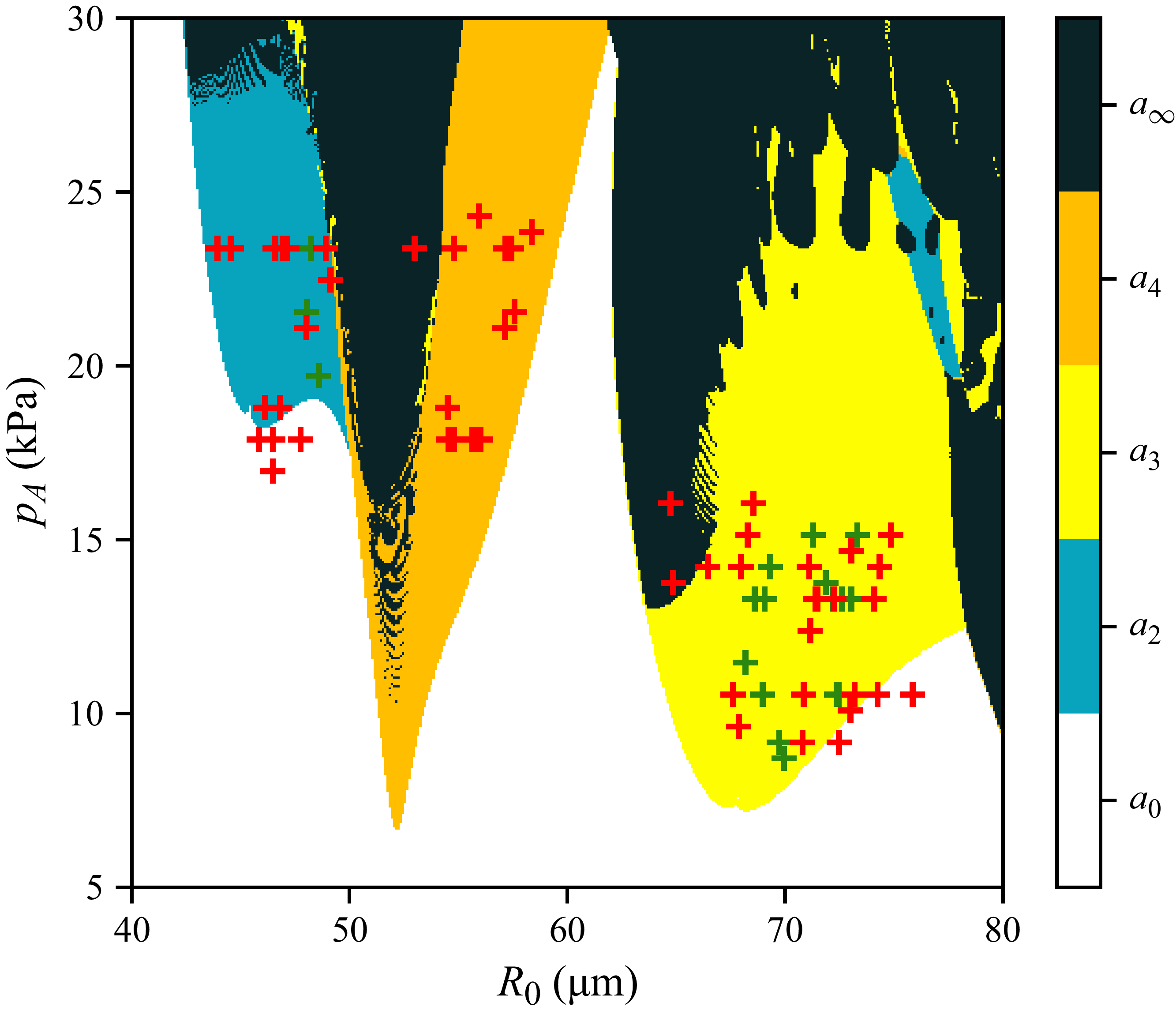
 R0=40
 80μm
 pa=5
 30kPa
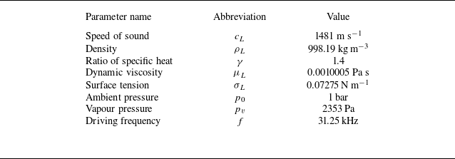

 R0=49.13μm
 pa=22.46kPa
 FA
 τ=t/T
 τ=1
 D
 DΣ

 R0=48.26μm
 pa=23.38kPa
 τ=1/T
 τ=1
 D
 DΣ
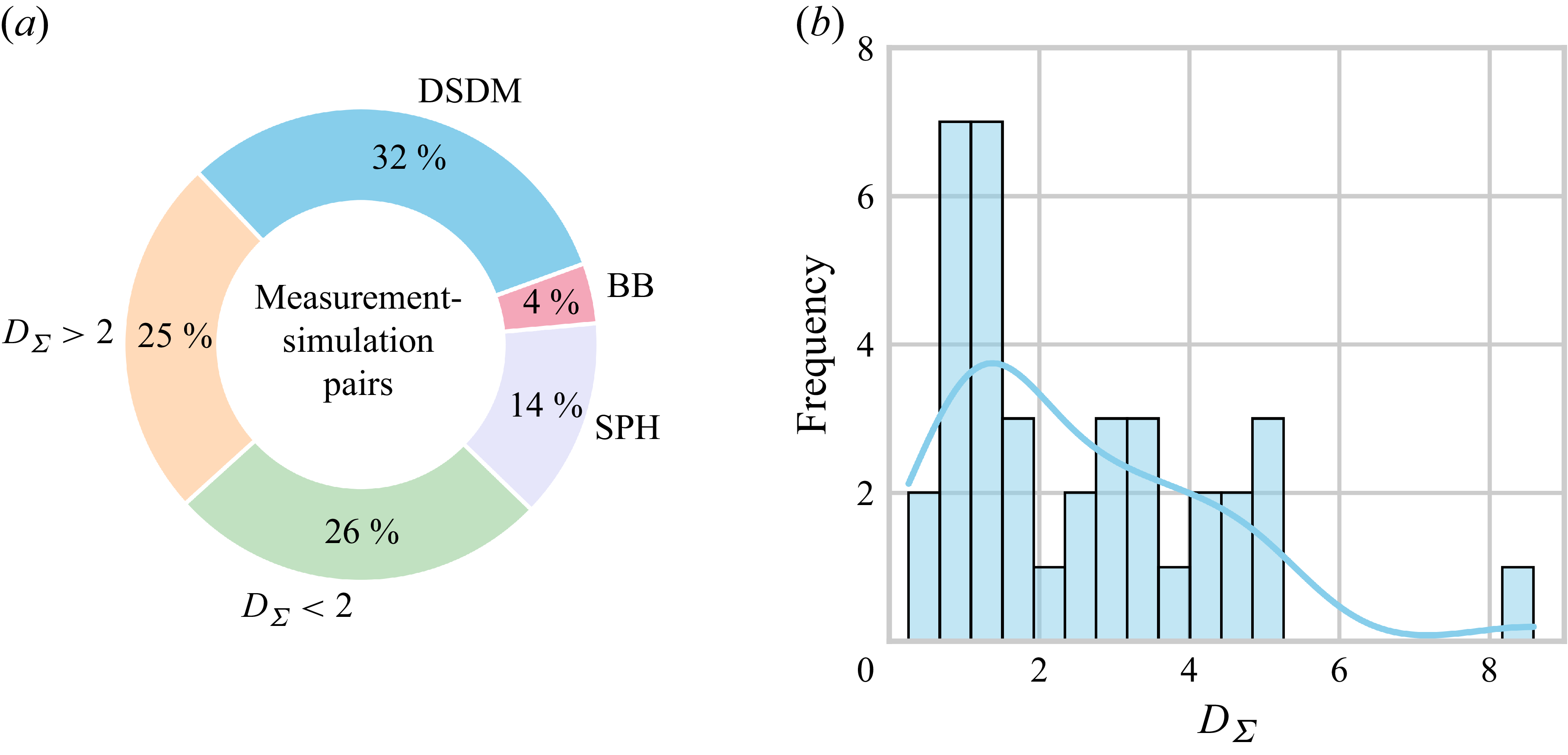
 DΣ<2
 DΣ>2
 DΣ
 DΣ<2
 DΣ>2
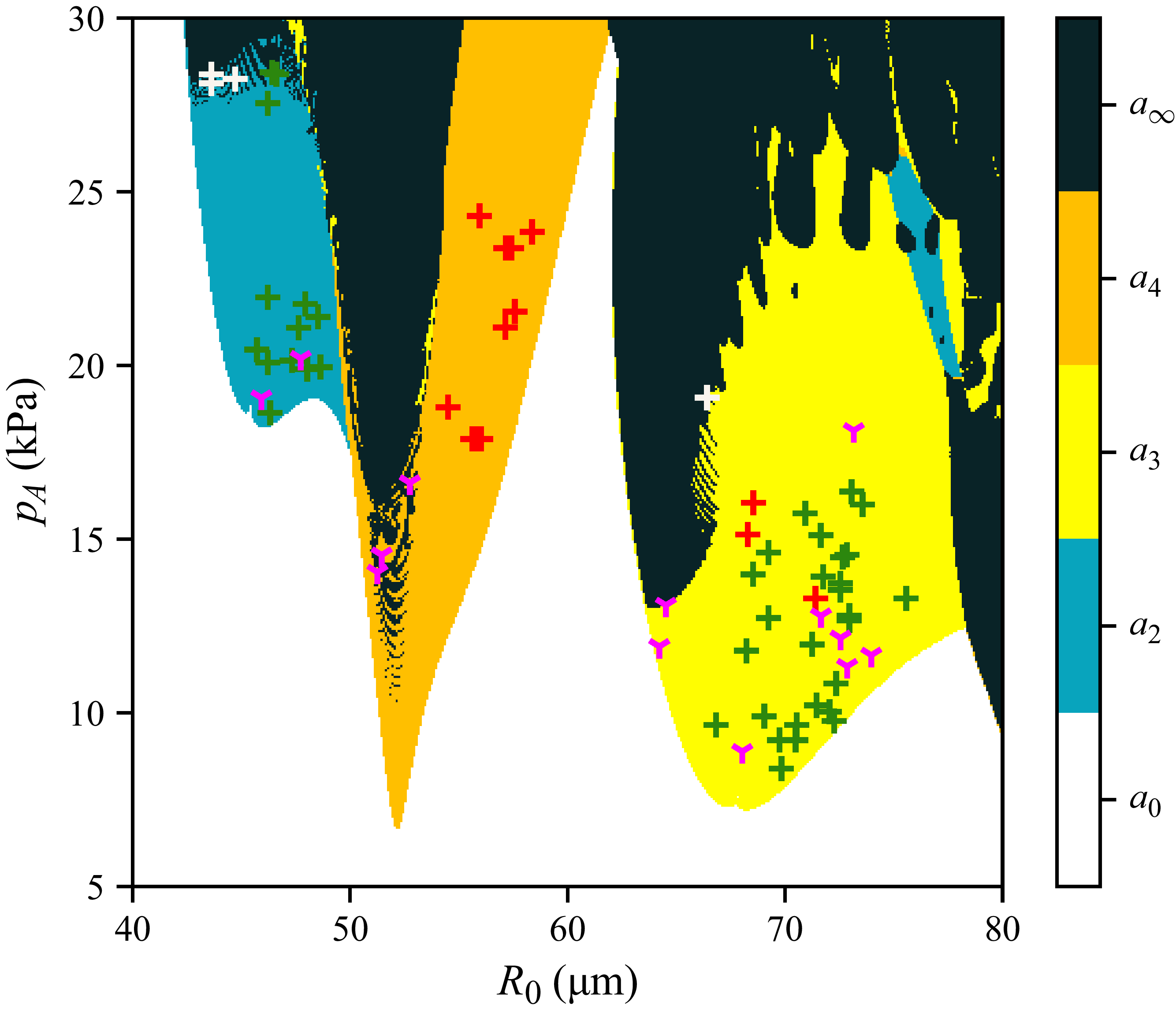
 R0=40−80
 μm
 pa=5−30
 kPa
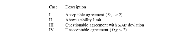

 DΣ
 DΣ=0.52

 DΣ
 DΣ=3.52

 R0=54.67μm
 16.81

 DΣ
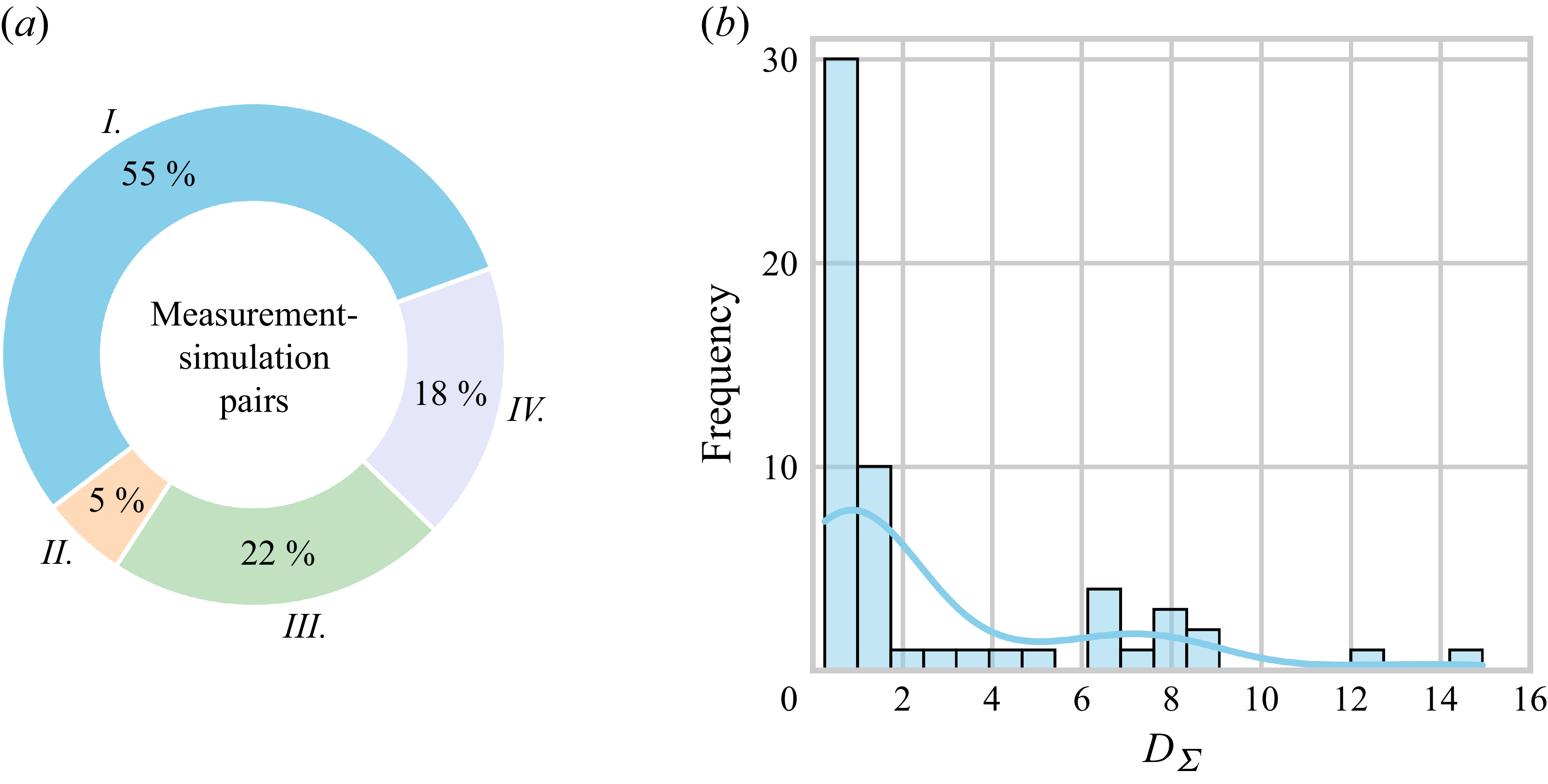
 DΣ

 α=20∘

 α
 R0=56 μm
 pA=17.5 kPa
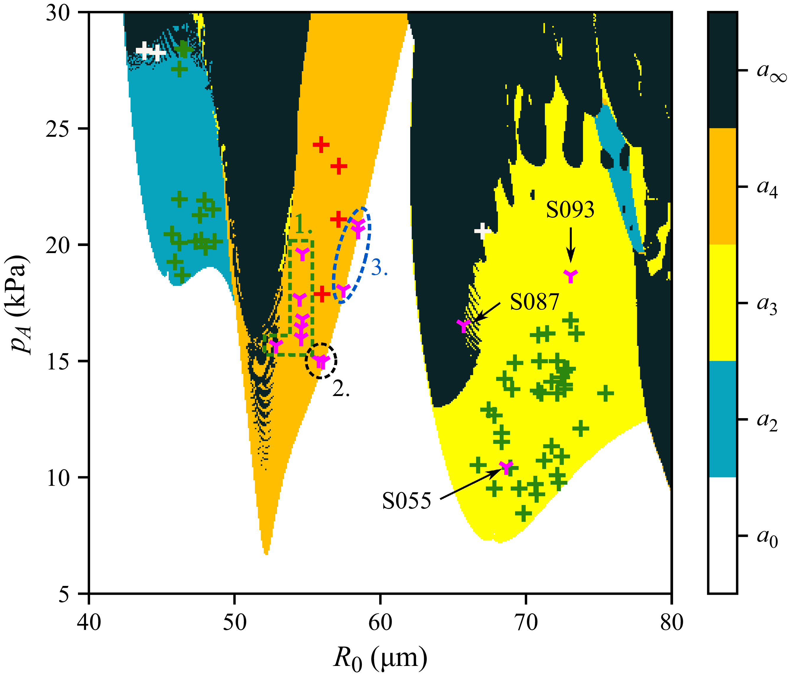
 R0=40
 80 μm
 pa=5
 30 kPa
 α

 R0=74.3μm
 pa=10.5kPa
 R0=73.87μm
 pa=11.6kPa
 R0=73.77μm
 pa=12.1kPa
 α=20∘

 R0=68.56μm
 pa=16.04kPa
 R0=68.64μm
 pa=10.45kPa
 α=−20∘

 R0=53.0μm
 pa=23.38kPa
 R0=52.86μm
 pa=15.68kPa
 α=4∘

 R0=55.85μm
 pa=17.88kPa
 R0=56.08μm
 pa=14.99kPa
 α=−20∘

 DΣ

 DΣ

 (d<0.025)

 (d<0.025)
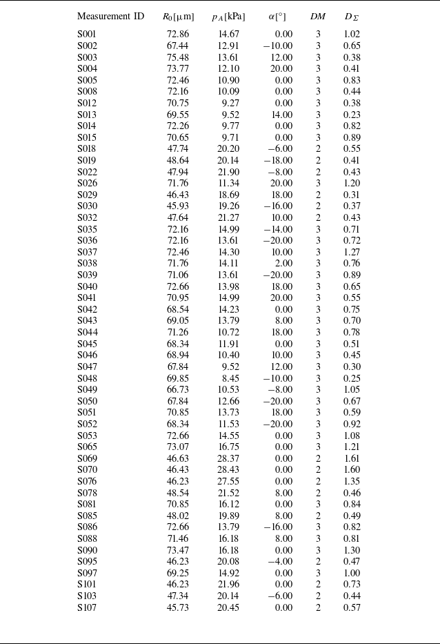
 R0
 pa
 α
 DΣ



