1. Introduction
An interesting feature of a finite amplitude weakly nonlinear single phase wavetrain is that such a wavetrain can be unstable to sideband perturbations (see Whitham Reference Whitham1967). For instability, the sidebands of the primary mode absorb energy from the primary mode itself. In the context of periodic gravity waves on infinite depth of water, Benjamin and Feir (see Benjamin & Feir Reference Benjamin and Feir1967; Benjamin Reference Benjamin1967; Feir Reference Feir1967) have investigated the experimental results of sideband instability. A physical interpretation for the inception of sideband instability, also called Benjamin–Feir instability, can well be comprehended through the study of weakly nonlinear wavetrains in infinite depth of water which initially contains waves of uniform wavelength. When the wave envelope has sinusoidal variations, the wavetrain at the crests of the envelope will propagate forwards more rapidly than the wavetrain at the troughs of the envelope owing to the nonlinearity of the wave motion. Therefore, wavenumbers will enhance in front of the envelope crests and diminish behind the envelope crests. Dispersive effects now cause energy to approach the crests of the envelope, causing the amplitude at the crests to enhance. This in turn expedites the sideband instability.
However, in the case of multiphase modes consisting of non-overlapping group velocity projections, the preceding studies (see Benney & Roskes Reference Benney and Roskes1969; Ablowitz Reference Ablowitz1972) propose that sideband instability may develop when any one mode is singly unstable. Using third-order nonlinear Schrödinger equations, Roskes (Reference Roskes1976a
,
Reference Roskesb
) has presented the modulational instability analysis of weakly nonlinear multiphase gravity wavetrains in infinite depth of water and remarked that modulational perturbation is restricted to a direction along which group velocity projections of two wavetrains overlap and the modulation will grow at a faster rate along this direction when
 $0\lt \theta \lt 70.5^{\circ }$
, where
 $\theta$
is the angle between the two propagation directions of two waves. A direction in which group velocity projections overlap is obtained by a unit vector
 $\boldsymbol{u}$
perpendicular to
 $\boldsymbol{c^{(1)}_g}{-}\boldsymbol{c^{(2)}_g}$
as in this case,
 $\boldsymbol{c^{(1)}_g}.\boldsymbol{u}=\boldsymbol{c^{(2)}_g}.\boldsymbol{u}$
, where
 $\boldsymbol{c^{(1)}_g}$
and
 $\boldsymbol{c^{(2)}_g}$
represent the group velocity of the first and second wavetrains, respectively. If the group velocity vectors
 $\boldsymbol{c^{(n)}_g}$
were equidirectional, then in this instance, we could prefer
 $\boldsymbol{u}$
to be perpendicular to
 $\boldsymbol{c^{(n)}_g}$
so that
 $\boldsymbol{c^{(n)}_g}.\boldsymbol{u}=0$
for all values of
 $n$
(see Roskes Reference Roskes1976b
). Later, Dhar & Das (Reference Dhar and Das1991) derived the fourth-order coupled NLE equations, which are an excellent starting point for the investigation of nonlinear water waves, for multiphase gravity wavetrains in deep water. Therefore, that paper is an extension of the paper made by Roskes to fourth-order in wave steepness. Subsequently, Dhar & Das (Reference Dhar and Das1993) further extended their previous paper to include the effect of capillarity and performed instability analysis for two Stokes capillary-gravity wavetrains when the amplitudes of two wavetrains are equal.
In the context of periodic water waves, the fourth-order analysis has always been found to be important as the results give significant physical insights on the properties of steady waves and their stability to sideband disturbances. For an example, Fang et al. (Reference Fang, Liu, Tang and Lin2023) exhibited that in the presence of a strongly sheared adverse current condition with uniform vorticity on water of finite depth, higher order solutions are effective in predicting a few properties of gravity waves as they match better with their experimental results. Again, as far as the stability properties of steady periodic water waves are concerned, the fourth-order perturbation analysis, carried out by Dhar & Kirby (Reference Dhar and Kirby2023), for capillary-gravity waves in the deep water case, exhibits notable deviations when compared with the third-order analysis and gives results that are more consistent with the exact numerical results. Finally, the paper of Dysthe (Reference Dysthe1979) is another strong example that describes the importance of considering fourth-order perturbation analysis, as he has clearly stated that a significant improvement can be achieved in the instability analysis to modulational perturbations of the gravity wavetrain in deep water. He has shown that the fourth-order results agree fairly well with the exact results of Longuet-Higgins (Reference Longuet-Higgins1978) and the experimental results of Benjamin & Feir (Reference Benjamin and Feir1967). The dominant new effect comes from the wave-induced mean flow response, whose component along the direction of wave propagation causes a local Doppler shift. This frequency shift then gives rise to changes in the instability properties of the wavetrain. In fact, the above-mentioned studies inspire us to perform the present fourth-order analysis in deep water.
The physical importance of the surface tension effects for the onset of modulational instability can be stated as follows. Using a perturbation expansion, Harrison (Reference Harrison1909) first studied the nonlinear behaviour of capillary-gravity waves in deep water. The question of the existence of plane progressive capillary-gravity waves has been first considered by Sekerzh-Zenkovich (Reference Sekerzh-Zenkovich1956). The most dominant wave–wave interaction among capillary waves is the three-wave interactions. Nevertheless, Shats, Punzmann & Xia (Reference Shats, Punzmann and Xia2010) exhibited experimentally that the nonlinear four-wave interactions caused by modulational instability can be dominant. To shed light on the physical processes governing the generation of steep wave events, they have taken into account the pure capillary waves. The novel and unexpected outcomes of their experiment on capillary waves is that the dominant wave interaction can be considered as a possible mechanism for the generation of freak waves, which occur due to the modulational instability and is an inseparable aspect of the nonlinear Schrödinger equation. Furthermore, in a series of three consecutive papers, Hogan (Reference Hogan1979, Reference Hogan1980, Reference Hogan1981) stated in the context of periodic steep capillary-gravity waves in deep water that surface tension produces a restoring force that cannot reasonably be neglected for water waves and obtained an unexpected result that the height of the capillary wave crest above the mean level is not a monotonic function of wave steepness. He has also shown that for pure capillary waves, the surface of the highest wave bends over and touches itself, enclosing a bubble of air, as has been found for capillary waves by Crapper (Reference Crapper1957). That experiment and analytical results motivate our study of modulational instability of finite amplitude capillary waves.
In the present paper, we focus our study on the modulational instability of weakly nonlinear multiphase capillary wavetrains in deep water starting from fourth-order coupled NLE equations. One of our objectives is to complete and extend the results of Dhar & Das (Reference Dhar and Das1993) on pure capillary wavetrains. To the best of our knowledge, there is no study on the modultional instability of capillary multiphase wavetrains in deep water. Herein, we present the multiphase modes when variations occur in a direction along which group velocity projections of two wavetrains overlap, so that the nonlinear interactive effects of two modes within the wavetrain are allowed to be strongly operative for a long period of time. Several studies have been devoted to the modulational instability of steadily propagating capillary wavetrains in deep water. Crapper (Reference Crapper1957) found an exact solution for two-dimensional periodic capillary waves in deep water and drew graphically the phase velocity as a function of wave amplitude. Kinnersley (Reference Kinnersley1976) then generalised Crapper’s exact solution for capillary waves and obtained two finite depth solutions involving elliptic functions. Constantin & Kartashova (Reference Constantin and Kartashova2009) have studied the effect of an underlying current on three wave interactions of capillary waves in finite depth and shown that waves in the presence of uniform vorticity are possible only for two-dimensional flows. Tiron & Choi (Reference Tiron and Choi2012) have also studied the instability of exact capillary wave solution, derived by Crapper (Reference Crapper1957), in deep water subject to two-dimensional disturbances. They have shown that Crapper’s capillary waves are linearly stable to superharmonic perturbations for all wave steepness and linearly unstable to subharmonic perturbations. Later, Murashige & Choi (Reference Murashige and Choi2021) investigated the three-dimensional instability of progressive capillary waves in deep water and remarked that for weakly three-dimensional superharmonic perturbations, the capillary waves are two-dimensionally stable but three-dimensionally unstable for almost all wave steepness. Recently, Kharif et al. (Reference Kharif, Abid, Chen and Hsu2025) derived a nonlinear Schrödinger equation for a single capillary wavetrain in arbitrary water depth with a shear current of constant vorticity and performed stability analysis of the weakly nonlinear periodic wavetrain.
The principal results and the significance of this work are as follows. (i) The dynamical fourth-order NLE equations are used to study the modulational instability (or the Benjamin–Feir instability) properties of weakly nonlinear capillary Stokes multiphase wavetrains in deep water. (ii) Results show that the instability region and the growth rates are larger when two carrier wavetrains are taken into account. (iii) We find the expression of the growth rate of instability for capillary wavetrains to transverse perturbations in deep water and provide the significant results. (iv) Particular attention is paid to the stability results of a capillary envelope soliton in infinite depth of water.
The plan of this paper is organised as follows. Following the introduction, in § 2, the formulation of the problem is presented. In § 3, the linear stability analysis of finite amplitude capillary multiphase wavetrains with respect to both longitudinal and transverse perturbations is carried out. A capillary solitary envelope solution in deep water is obtained in § 4 and, finally, the chief outcomes are summarised in § 5.
2. Fundamental equations and the coupled NLE equations for pure capillary waves
We consider the evolution of the weakly nonlinear progressive capillary wavetrains propagating steadily on the free surface of a fluid of infinite depth. The undisturbed free surface corresponds to the plane
 $z=0$
, where
 $z$
is the vertical coordinate pointed upwards. The Cartesian coordinates
 $x,y$
are situated on the plane of the undisturbed free surface. It is assumed that the two wavetrains propagate on the
 $(x,y)$
plane with wavenumbers
 $k_1$
and
 $k_2$
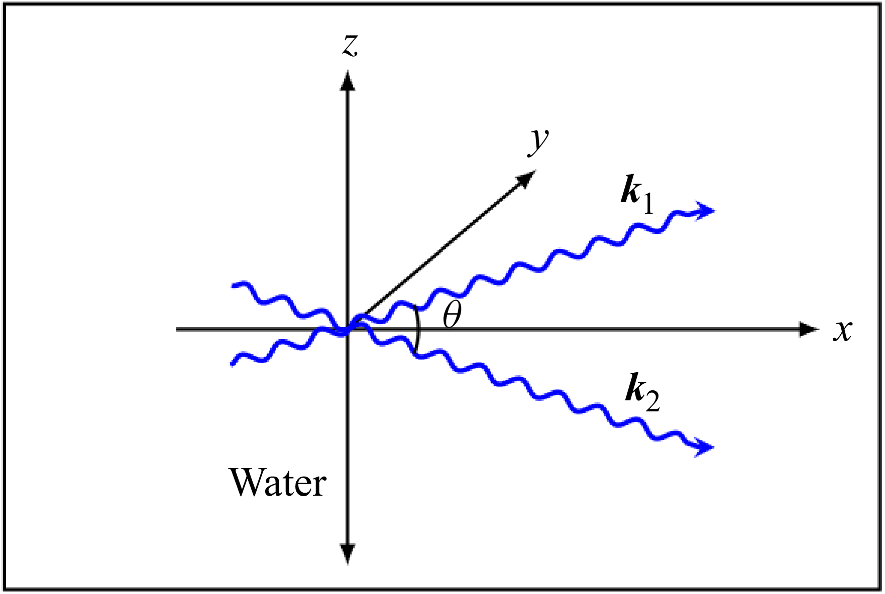
, as shown in figure 1. We choose the
 $x$
-axis in a direction along which group velocity projections of the two wavetrains overlap and take the modulations along this line.
Schematic description of the physical problem of two wavetrains.

The system of governing equations belongs to the Laplace equation given by (2.1) together with kinematic and dynamic boundary conditions (2.2), (2.3) and bottom condition (2.4) for an inviscid, incompressible and irrotational fluid of infinite depth with a free surface under the influence of capillarity, and may be formulated as
 \begin{align} \nabla^2\varPhi +\frac {\partial ^2\varPhi }{\partial z^2}&=0,\quad -\infty \lt z\lt \eta (x,y,t), \end{align}
 \begin{align} \frac {\partial \eta }{\partial t}-\frac {\partial \varPhi }{\partial z}&=\boldsymbol{\nabla }\eta .\boldsymbol{\nabla }\varPhi ,\quad \text{at}\,\,z=\eta (x,y,t), \end{align}
 \begin{align} \frac {\partial {\varPhi }}{\partial {t}}&=-\frac {1}{2}\left [ \!(\boldsymbol{\nabla }{\varPhi })^{2}+\left (\frac {\partial \varPhi }{\partial z}\right )^2 \!\right ]+T\frac {\big[\eta _{xx}\big(1+\eta ^2_{y}\big)+\eta _{yy}\left(1+\eta ^2_{x}\right)-2\eta _{xy}\eta _{x}\eta _{y}\big]}{\big(1+\eta ^2_{x}+\eta ^2_{y}\big)^{3/2}},\nonumber \\ & \qquad \qquad \qquad \qquad \qquad \qquad \qquad \qquad \qquad \qquad \qquad \text{at}\,\, z=\eta (x,y,t) ,\end{align}
 \begin{align} \boldsymbol{\nabla }\varPhi &=0,\quad \text{at}\,\,z\rightarrow -\infty, \end{align}
where
 $(x,y)=\boldsymbol{x}$
are the horizontal coordinates,
 $\eta (x,y,t)$
is the free surface elevation,
 $\varPhi (x,y,z,t)$
is the velocity potential of capillary wavetrain,
 $\boldsymbol{\nabla }=( {\partial }/{\partial x}, {\partial }/{\partial y})$
is the horizontal gradient operator and
 $T$
is the ratio of the surface tension coefficient to the fluid density. One can observe that the dynamic boundary condition (2.3) at the free surface for pure capillary wavetrains is different from the corresponding boundary condition for gravity wavetrains due to the presence of surface tension coefficient
 $T$
and the absence of gravity acceleration
 $g$
, whereas the remaining equation and the boundary conditions are the same for both the systems.
The dispersion relations of the linearised (2.1)–(2.4) for two capillary wavetrains with wavenumbers
 $k_1$
,
 $k_2$
and frequencies
 $\sigma _1$
,
 $\sigma _2$
are
 \begin{equation} \sigma ^2_i=T \big(k^2_{ix}+k^2_{iy}\big)^{3/2}=Tk^3,\quad (i=1,\,2). \end{equation}
An interesting case is obtained if we consider the simplifying assumption that the wavenumbers of two wavetrains are equal so that
 $\lvert \boldsymbol{k_1}\rvert =\lvert \boldsymbol{k_2}\rvert =k$
(say). We take the common wavenumber to be equal to
 $k_0$
, the characteristic wavenumber. Therefore, we have
 $k=\lvert \boldsymbol{k_1}\rvert =\lvert \boldsymbol{k_2}\rvert =1$
and, hence, (2.5) becomes
 \begin{equation} \sigma ^2=T. \end{equation}
To obtain the dispersive and nonlinear coefficients of the coupled NLE equations for pure capillary wavetrains, we have used the expressions derived by Dhar & Das (Reference Dhar and Das1993) for capillary-gravity wavetrains when
 $\kappa =k^2T/g$
tends to infinity. Herein,
 $\kappa$
denotes the dimensionless capillary number similar to the inverse of the Bond number. The summary of derivations of (2.7) and (2.8) are given in Appendix A. The limit of the dispersive coefficients can be found easily, whereas the limit of the nonlinear coefficients cannot be readily obtained as this involves some algebra. The fourth-order coupled NLE equations for the complex envelopes
 $\eta _1$
,
 $\eta _2$
of two wavetrains are given by
 \begin{align} & i\frac {\partial \eta _1}{\partial \tau }+\gamma _1\frac {\partial ^2\eta _1}{\partial X^2}+i\gamma _2\frac {\partial ^3\eta _1}{\partial X^3}=\big(\beta _{11}\lvert \eta _1\rvert ^2+\beta _{12}\lvert \eta _2\rvert ^2\big)\eta _1 +i\big(\lambda _{1}\lvert \eta _1\rvert ^2+\lambda _{2}\lvert \eta _2\rvert ^2\big)\frac {\partial \eta _1}{\partial X}\nonumber \\ &\quad+i\lambda _3\eta ^2_1\frac {\partial \eta ^*_1}{\partial X}+i\lambda _4\eta _1\eta ^*_2\frac {\partial \eta _2}{\partial X}+i\lambda _5\eta _1\eta _2\frac {\partial \eta ^*_2}{\partial X}+\varLambda \eta _1 H\left [\frac {\partial }{\partial X}\big(\lvert \eta _1\rvert ^2+\lvert \eta _2\rvert ^2\big)\right ]\!, \end{align}
 \begin{align} & i\frac {\partial \eta _2}{\partial \tau }+\gamma _1\frac {\partial ^2\eta _2}{\partial X^2}+i\gamma _2\frac {\partial ^3\eta _2}{\partial X^3}=\big(\beta _{12}\lvert \eta _1\rvert ^2+\beta _{11}\lvert \eta _2\rvert ^2\big)\eta _2 +i\big(\lambda _{1}\lvert \eta _2\rvert ^2+\lambda _{2}\lvert \eta _1\rvert ^2\big)\frac {\partial \eta _2}{\partial X}\nonumber \\ &\quad+i\lambda _3\eta ^2_2\frac {\partial \eta ^*_2}{\partial X}+i\lambda _4\eta _2\eta ^*_1\frac {\partial \eta _1}{\partial X} +i\lambda _5\eta _1\eta _2\frac {\partial \eta ^*_1}{\partial X}+\varLambda \eta _2 H\left [\frac {\partial }{\partial X}\big(\lvert \eta _1\rvert ^2+\lvert \eta _2\rvert ^2\big)\right ]\!. \end{align}
It is to be noted that the two coefficients
 $\gamma _1$
and
 $\beta _{12}$
are very important for obtaining the instability results. Therefore, we have presented the calculation of these coefficients in detail in Appendix B when
 $\kappa$
tends to infinity. The coefficients appearing in (2.7) and (2.8) are given in Appendix C. Here,
 $\eta _1,\,\eta _2$
represent the complex amplitudes corresponding to the first and second wavetrains, respectively. To obtain the above-mentioned equations, we transform to moving coordinates and introduce the variables
 \begin{align} X=\epsilon (x-c_gt),\quad \tau =\epsilon ^2t, \end{align}
where
 $\epsilon$
is a small ordering parameter that characterises both the wave amplitude and the slow modulations, and
 $c_g$
is the component of the group velocity of either wavetrain along the
 $x$
-axis and is given by
 \begin{align} c_g=\cos \frac {\theta }{2} \left (\frac {{\rm d}\sigma }{{\rm d}k}\right )_{k=1}, \end{align}
where
 $ ( {{\rm d}\sigma }/{{\rm d}k})_{k=1}$
is to be calculated from (2.5) and
 $\theta$
is the angle between two wavenumber vectors
 $\boldsymbol{k_1}$
and
 $\boldsymbol{k_2}$
. Additionally,
 $H$
is the one-dimensional version of the Hilbert transform given by
 \begin{align} H[\chi (X)]=\frac {1}{\pi } P\int _{-\infty }^{\infty }\frac {\chi (X^{\prime })\,{\rm d}X^{\prime }}{X^{\prime }-X}. \end{align}
Here,
 $P$
indicates the principal value of the integral. In this work, we give some of the results concerning the interaction between two modes when modulation takes place in a direction along which group velocity projections overlap.
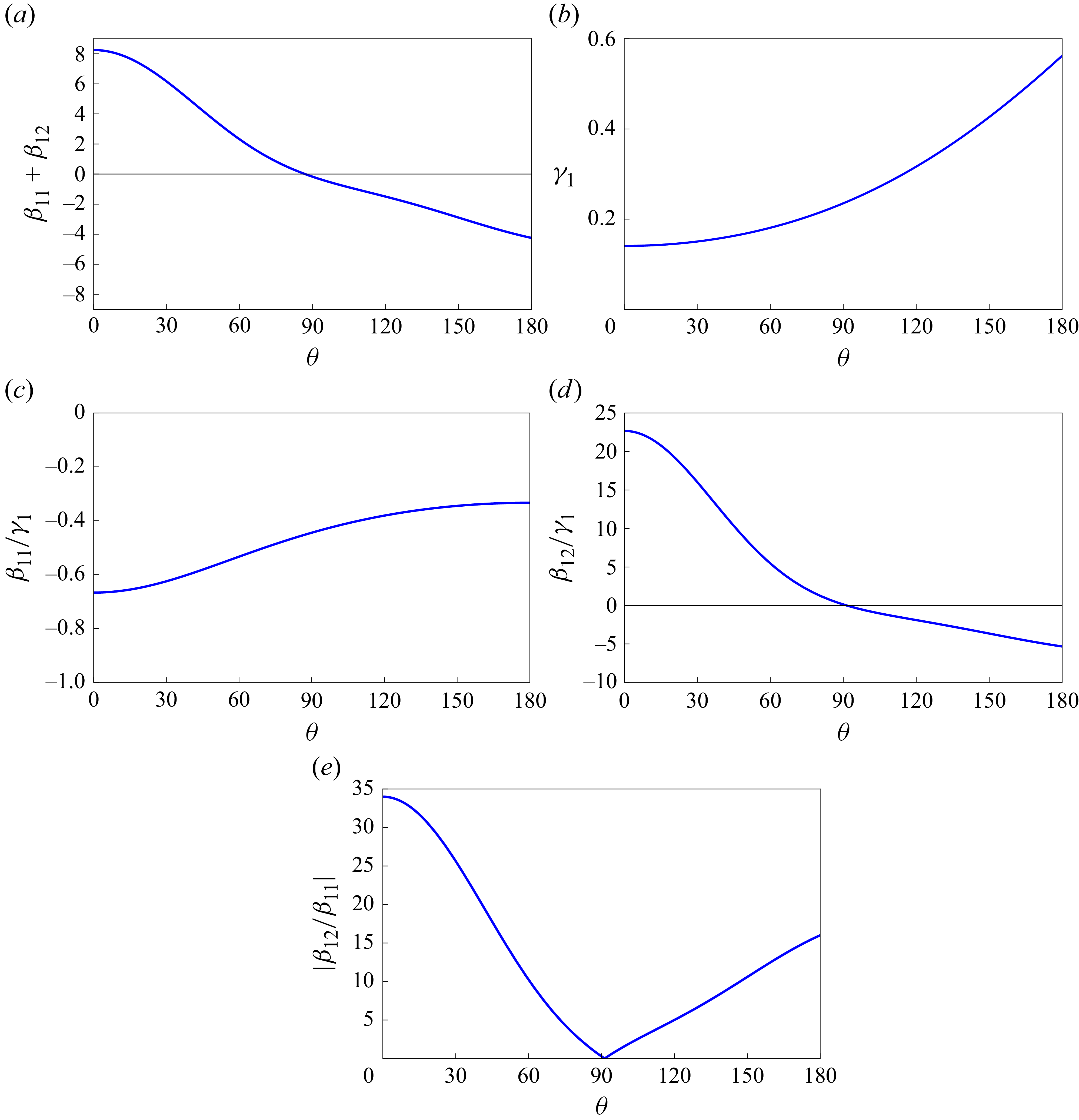
Figure 2
 $(a,b)$
shows the variation of the coefficients
 $\beta _{11}+\beta _{12}$
and
 $\gamma _1$
as a function of angle
 $\theta$
. The coefficient
 $\beta _{11}+\beta _{12}$
changes sign at
 $\theta \approx 86.86^{\circ }$
from positive to negative. This coefficient has some consequences on the instability properties of two capillary wavetrains, as shown in the next two sections. One can observe that the coefficient
 $\gamma _1$
is positive for all values of
 $\theta$
and, therefore, the system of two wavetrains is stable in the range
 $0\leqslant \theta \leqslant 86.86^{\circ }$
. To evaluate the relative relevance of the nonlinear terms for distinct angles, we plot in figure 2
 $(c,d)$
the ratios
 $\beta _{11}/\gamma _1$
and
 $\beta _{12}/\gamma _1$
against
 $\theta$
. We exhibit the absolute value of the ratio between the coefficients of the nonlinear terms in figure 2
 $(e)$
. It is found that the nonlinearity owing to the cross-interaction term dominates for
 $\theta \lt 86.86^{\circ }$
, whereas for
 $\theta \gt 86.86^{\circ }$
, the self-interaction nonlinearity dominates. For
 $\theta \approx 86.86^{\circ }$
, the nonlinear coefficients
 $\beta _{11}$
and
 $\beta _{12}$
are equal. For
 $\theta \approx 91.30^{\circ }$
, the cross-interaction term
 $\beta _{12}$
takes the value zero and consequently the system becomes uncoupled.
(a,b) Plot of nonlinear and dispersive coefficients as a function of
 $\theta$
; (c,d) plot of ratio between nonlinear and dispersive coefficients as a function of
 $\theta$
; (e) plot of ratio between cross-interaction and self-interaction coefficients.

In the next section, we intend to present the stability analysis of uniform wavetrains based on the coupled NLE equations, which consists in describing the different coefficients in front of the dispersive, self-interaction and cross-interaction terms.
3. Modulational instability of Stokes capillary multiphase wavetrains
Herein, we study the instability of capillary Stokes wavetrains when the restoring force is derived from surface tension alone. We first present the stability analysis with respect to longitudinal modulation and then with respect to both longitudinal and transverse modulations. We present some of the analytical results of an analysis of the interaction of two wavetrains in deep water when modulations develop in a direction along which group velocity projections overlap.
3.1. Stability analysis with respect to longitudinal modulation
Using a multiscale expansion, Roskes (Reference Roskes1976a
) derived the coupled nonlinear Schrödinger equations in the context of two-phase gravity wavetrains in deep water and shown that these equations for
 $\eta _1$
and
 $\eta _2$
are very convenient for investigating the stability analysis of the uniform Stokes wavetrains. He has also stated that the Stokes wavetrains are unstable to modulational perturbations. For a review of basic notion, physical interpretation and detailed history concerning the onset of modulation instability of nonlinear waves, the readers are referred to the papers of Zakharov & Ostrovsky (Reference Zakharov and Ostrovsky2009) and Roskes (Reference Roskes1976b
).
The solutions of the uniform Stokes wavetrains of (2.7) and (2.8) are given by
 \begin{align} \begin{aligned} &\eta _1=\eta ^{(0)}_1= \frac {\eta _{01}}{2}\exp \left [\frac {-i}{4}\big(\beta _{11}\eta ^2_{01}+\beta _{12}\eta ^2_{02}\big)\tau \right ]\!, \\ &\eta _2=\eta ^{(0)}_2= \frac {\eta _{02}}{2}\exp \left [\frac {-i}{4}\big(\beta _{11}\eta ^2_{02}+\beta _{12}\eta ^2_{01}\big)\tau \right ]\!, \end{aligned} \end{align}
where
 $\eta _{01}$
,
 $\eta _{02}$
are real constants and represent the wave steepness of the two wavetrains. The amplitude dependent frequency shifts for the two wavetrains are given by
 $\Delta \sigma _1=(\beta _{11}\eta ^2_{01}+\beta _{12}\eta ^2_{02})/4$
and
 $\Delta \sigma _2=(\beta _{11}\eta ^2_{02}+\beta _{12}\eta ^2_{01})/4$
. As the two wavetrains have the same wavenumber equal to one, the change in the phase speeds of the two wavetrains becomes
 \begin{align} \begin{aligned} &\Delta v_1=\frac {\Delta \sigma _1}{\lvert \boldsymbol{k_1}\rvert }=\Delta \sigma _1=\frac {1}{4}\big(\beta _{11}\eta ^2_{01}+\beta _{12}\eta ^2_{02}\big), \\ &\Delta v_2=\frac {\Delta \sigma _2}{\lvert \boldsymbol{k_2}\rvert }=\Delta \sigma _2=\frac {1}{4}\big(\beta _{11}\eta ^2_{02}+\beta _{12}\eta ^2_{01}\big). \end{aligned} \end{align}
It is important to note that the change in the phase speeds of each wavetrain can be divided into two parts. In (3.2), the first correction to
 $v_1$
is given by
 $\beta _{11}\eta ^2_{01}/4$
, which is the well-known Stokes (Reference Stokes1847) correction. This term is due to the nonlinearity of the wavetrain itself and is present even in the absence of the other wavetrain. Again, the second correction is given by
 $\beta _{12}\eta ^2_{02}/4$
and is completely due to the presence of the other wavetrain, and is the same order as the usual Stokes correction.
Further, the relative change in phase speed
 $\Delta {\tilde v_1}$
of the first wavetrain due to the presence of the second wavetrain is given by
 \begin{align} \Delta {\tilde v_1}=\frac {\beta _{12}}{4}\eta ^2_{02}. \end{align}
A similar expression for the phase speed
 $\Delta {\tilde v_2}$
of the second wavetrain due to the presence of the first wavetrain is given by
 \begin{align} \Delta {\tilde v_2}=\frac {\beta _{12}}{4}\eta ^2_{01}. \end{align}
A linearised stability analysis of two uniform wavetrains may be investigated by introducing the following infinitesimal perturbations:
 \begin{align} &\eta _1=\eta ^{(0)}_1 \big[1+{\tilde \eta _1}(X,\tau )\big ],\nonumber \\&\eta _2=\eta ^{(0)}_2\big [1+{\tilde \eta _2}(X,\tau )\big ]. \end{align}
Inserting (3.5) into (2.7) and (2.8), linearising with respect to
 $\tilde \eta _1$
,
 $\tilde \eta _2$
,
 $\tilde \eta _1^{*}$
,
 $\tilde \eta _2^{*}$
, and separating the equations after setting
 ${\tilde \eta _1}=\eta ^{(1)}_r+i\eta ^{(1)}_i$
,
 ${\tilde \eta _2}=\eta ^{(2)}_r+i\eta ^{(2)}_i$
, in which
 $\eta ^{(1)}_r$
,
 $\eta ^{(1)}_i$
,
 $\eta ^{(2)}_r$
,
 $\eta ^{(2)}_i$
are real quantities, we obtain four linear algebraic equations for the four latter quantities. We assume the time dependence of
 $\eta _r^{(m)}$
,
 $\eta _i^{(m)}$
 $(m=1,\,2)$
to be of the form
 $\exp (-i\tilde \varOmega \tau )$
and then take the Fourier transform of the four linear equations with respect to
 $X$
defined by
 \begin{align} &\left(\hat \eta _{r}^{(1)},\,\hat \eta _{i}^{(1)},\,\hat \eta _{r}^{(2)},\,\hat \eta _{i}^{(2)} \right)=\frac {1}{\sqrt {2\pi }} \int _{-\infty }^\infty \left(\eta _{r}^{(1)},\,\eta _{i}^{(1)},\,\eta _{r}^{(2)},\,\eta _{i}^{(2)} \right)\exp ({-}\textit{ipX}){\rm d}X. \end{align}
The condition for the existence of a non-trivial solution to the four linear homogeneous equations gives the following nonlinear dispersion relation, where we assume that the amplitudes of two wavetrains are equal, that is,
 $\eta _{01}=\eta _{02}=\alpha$
,
 \begin{align} & A_1=-\left [\frac {\alpha ^2(\lambda _1+\lambda _2+\lambda _4)p}{4}\right ]\pm \left [A _2\left \{A_2+\frac {(\beta _{11}+\beta _{12}-2\varLambda \lvert p\rvert )\alpha ^2}{2}\right \}\right ]^{1/2}, \end{align}
where
 \begin{align} \begin{aligned} &A_1=\varOmega -c_{\textit{gp}}+\gamma _2p^3, \\ &A_2=\gamma _1p^2, \end{aligned} \end{align}
with
 $\varOmega =\tilde \varOmega + c_{\textit{gp}}$
. Note that this relation is obtained in view of the transformation (2.9). The derivation of the above-mentioned result as a general case is presented in Appendix D. Here,
 $p$
and
 $\varOmega$
represent the perturbed wavenumber and frequency, respectively. From (3.7), it is observed that perturbation to the spatially uniform solutions of amplitudes
 $\eta _i\,(i=1,2)$
grows exponentially and is therefore unstable when
 \begin{align} 2\gamma _1p^2+(\beta _{11}+\beta _{12}-2\varLambda \lvert p\rvert )\alpha ^2\lt 0, \end{align}
which leads to a complex valued
 $\varOmega$
. The analysis reveals that there are several wavenumber bands within which the capillary wavetrains are unstable to sideband perturbations. Within these unstable sidebands, the water wave motion depends essentially on the existence of capillary envelope solitons and therefore the uniform wavetrains do not exist. In fact, detection of the modulational instability and solitons generation in the capillary regime may be offset by the quick viscous dissipation occurring at large wavenumbers. By an examination of the coefficients
 $\beta _{11}+\beta _{12},\,\gamma _1$
and figure 2, one can observe that the above-mentioned condition is fulfilled when
 $\theta$
lies in the range
 $86.86^{\circ }\lt \theta \leqslant 180^{\circ }$
and the growth rate of instability, expressed as the imaginary part of
 $\varOmega$
, becomes
 \begin{align} \varOmega _{i}=\frac {p}{\sqrt {2}}\big [\gamma _1(2\varLambda \lvert p\rvert -\beta _{11}-\beta _{12})\alpha ^2-2\gamma ^2_1p^2\big ]^{1/2}. \end{align}
From (3.9), the instability bandwidth is
 \begin{align} p=\left [\left \{\frac {-(\beta _{11}+\beta _{12})}{2\gamma _1}\right \}^{1/2}+\frac {\varLambda }{2\gamma _1}\alpha \right ] \alpha , \end{align}
which shows that for instability,
 \begin{align} (\beta _{11}+\beta _{12})\lt 0 \end{align}
as
 $\gamma _1\gt 0$
for all values of
 $\theta$
. It is observed that for capillary wavetrains, instability occurs when
 $86.86^{\circ }\lt \theta \leqslant 180^{\circ }$
, whereas for gravity wavetrains, instability occurs when
 $\theta$
lies either in the range
 $0\lt \theta \lt 70.5^{\circ }$
or in
 $136.1^{\circ }\lt \theta \leqslant 180^{\circ }$
(see Roskes Reference Roskes1976a
; Dhar & Das Reference Dhar and Das1991).
At marginal stability,
 $\varOmega _r$
, the real part of
 $\varOmega$
takes the form
 \begin{align} \varOmega _r=c_g\left [\left \{\frac {-(\beta _{11}+\beta _{12})}{2\gamma _1}\right \}^{1/2}+\frac {\varLambda }{2\gamma _1}\alpha \right ] \alpha. \end{align}
The growth rate of instability takes a maximum value for perturbation wavenumber
 $p_m$
given by
 \begin{align} p_m= \left [\frac {-(\beta _{11}+\beta _{12})}{4\gamma _1}\right ]^{1/2} \alpha +\frac {3\varLambda }{8\gamma _1}\alpha ^2. \end{align}
The maximum growth rate of instability
 $\varOmega _{\textit{im}}$
is then
 \begin{align} \varOmega _{\textit{im}}= \frac {\lvert \beta _{11}+\beta _{12}\rvert \alpha ^2}{4}\left [1-\frac {2\varLambda \alpha }{\sqrt {-\gamma _1(\beta _{11}+\beta _{12})}}\right ]\!. \end{align}
Note that in the fourth-order NLE equations (2.7) and (2.8), the Hilbert transform terms disappear when
 $\theta =180^{\circ }$
and thereby fourth-order contribution in the expression of
 $\varOmega _{\textit{im}}$
does not affect the maximum growth rate instability.
Furthermore, the real value of
 $\varOmega$
corresponding to
 $p_m$
becomes
 \begin{align} \varOmega _{\textit{rm}}=c_g\left [\left \{\frac {-(\beta _{11}+\beta _{12})}{4\gamma _1}\right \}^{1/2}+\frac {3\varLambda }{8\gamma _1}\alpha \right ] \alpha , \end{align}
where
 $\varOmega _{\textit{rm}}$
represents the normalised frequency separation of the fastest growing sideband component. It is important to note that in (3.11), (3.13), (3.14) and (3.16), the key element is the sign of the product
 $\gamma _1(\beta _{11}+\beta _{12})$
at
 $O(\alpha )$
, which can be shown to be equivalent to Lighthill (Reference Lighthill1965)’s condition.
The results corresponding to third-order equations are given by
 \begin{align} \frac {\varOmega _i}{\alpha ^2} &=\frac {1}{\sqrt {2}}\left (\frac {p}{\alpha }\right ) \left [-\gamma _1\left \{(\beta _{11}+\beta _{12})+2\gamma _1\left (\frac {p}{\alpha }\right )^2\right \}\right ]^{1/2}, \end{align}
 \begin{align} p&= \left \{\frac {-(\beta _{11}+\beta _{12})}{2\gamma _1}\right \}^{1/2}\alpha , \\[-28pt] \nonumber \end{align}
 \begin{align} \varOmega _{\textit{im}}&= \frac {\lvert \beta _{11}+\beta _{12}\rvert \alpha ^2}{4} \\[-2pt] \nonumber \end{align}
and
 \begin{align} \varOmega _{\textit{rm}}=c_g\left \{\frac {-(\beta _{11}+\beta _{12})}{4\gamma _1}\right \}^{1/2}\alpha. \end{align}
Notice that when modulations take place in directions along which group velocity projections do not overlap, preceding studies show that maximum instability growth rates are provided by that of the most unstable single-phase mode. For physical interpretation, we observe herein two types of interaction affecting the results. As a first point, as is well known from Lighthill (Reference Lighthill1965), the relative signs of the envelope frequency dispersion term given by
 $\gamma _1(\eta _1)_{\textit{XX}}$
and the cubic nonlinear term
 $[\beta _{11}{\lvert \eta _1\rvert }^2+\beta _{12}{\lvert \eta _2\rvert }^2]\eta _1$
govern the entire instability of the solution. The analysis reveals that there exists a band of stable wavetrains for which the product
 $\gamma _1(\beta _{11}+\beta _{12})$
is positive. As a second point, the modifications to the modulational instability characteristics that occur at fourth-order can be found to derive from an interaction between the mean flow term involving Hilbert transform and the frequency dispersion term
 $\gamma _1(\eta _1)_{\textit{XX}}$
, as shown from the second term of the expression
 $p$
given by (3.11). Finally, significance has been devoted to the nonlinear terms whose coefficients are
 $\lambda _1$
,
 $\lambda _2$
and
 $\lambda _4$
of (2.7). In view of (3.7), we find that they give the real
 $O(\alpha ^2)$
correction to the frequency of sufficiently large plane perturbations to the wavetrains.
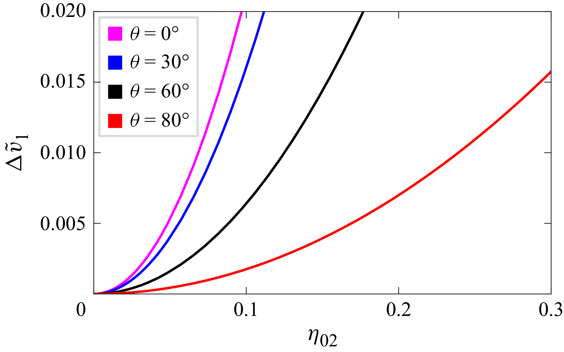
We have plotted
 $\Delta \tilde v_1$
given by (3.3) in figure 3 as a function of
 $\eta _{02}$
for some values of
 $\theta$
. It is observed that the relative change in phase speed
 $\Delta \tilde v_1$
of the first wavetrain increases as the wave steepness
 $\eta _{02}$
increases, whereas it decreases with the increase of
 $\theta$
.
Relative change in phase speed
 $\Delta \tilde v_1$
of the first wavetrain as a function of
 $\eta _{02}$
for different values of
 $\theta$
.

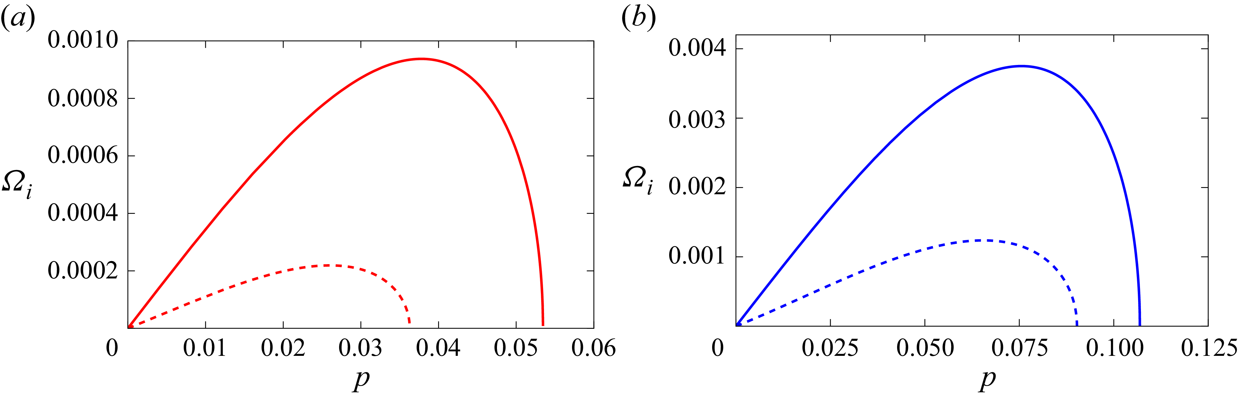
In figure 4, we have drawn the instability growth rate
 $\varOmega _i$
given by (3.10) as a function of perturbed wavenumber
 $p$
for several values of wave steepness
 $\alpha$
and angle
 $\theta$
. These figures illustrate that the growth rate increases with the increase of
 $\theta$
as well as the wave steepness
 $\alpha$
. It is found that the effect of the fourth-order term is to enhance the growth rate of instability. Figure 5 suggests the fact that the instability growth rate for two capillary wavetrains is much higher than that for a single capillary wavetrain, consistent with the results of Onorato, Osborne & Serio (Reference Onorato, Osborne and Serio2006) for two obliquely propagating gravity wavetrains in deep water.
Plot of instability growth rate
 $\varOmega _i$
as a function of
 $p$
for several values of
 $\theta$
.
 $(a)\, \alpha =0.1;\,(b)\, \alpha =0.2$
.
 $\alpha$
denotes the amplitude of two wavetrains. Third-order result (dashed line) and fourth-order result (solid line).

Plot of growth rate
 $\varOmega _i$
as a function of
 $p$
for longitudinal perturbation of a single capillary wavetrain (dashed line) and of two capillary wavetrains (solid line).
 $(a)\,\alpha =0.05$
;
 $\,(b) \,\alpha =0.1$
.

The perturbed frequency
 $\varOmega _r$
at marginal stability given by (3.13) is plotted against
 $\alpha$
for some values of
 $\theta$
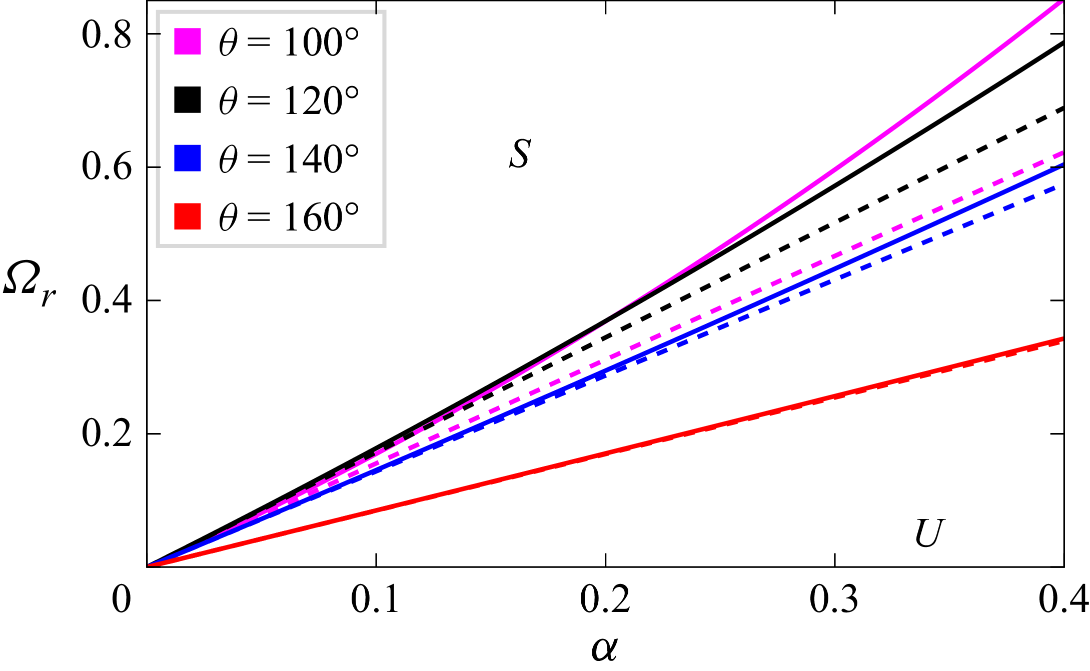
, as depicted in figure 6. These graphs exhibit deviations of the results obtained from third-order and fourth-order equations and the deviation increases with the decrease of
 $\theta$
.
Curves of marginal stability as a function of
 $\alpha$
for different values of
 $\theta$
. Third-order result (dashed line) and fourth-order result (solid line).
 $S$
and
 $U$
represent the stable and unstable regions.

Using (3.15) and (3.19), the maximum growth rate of instability
 $\varOmega _{\textit{im}}$
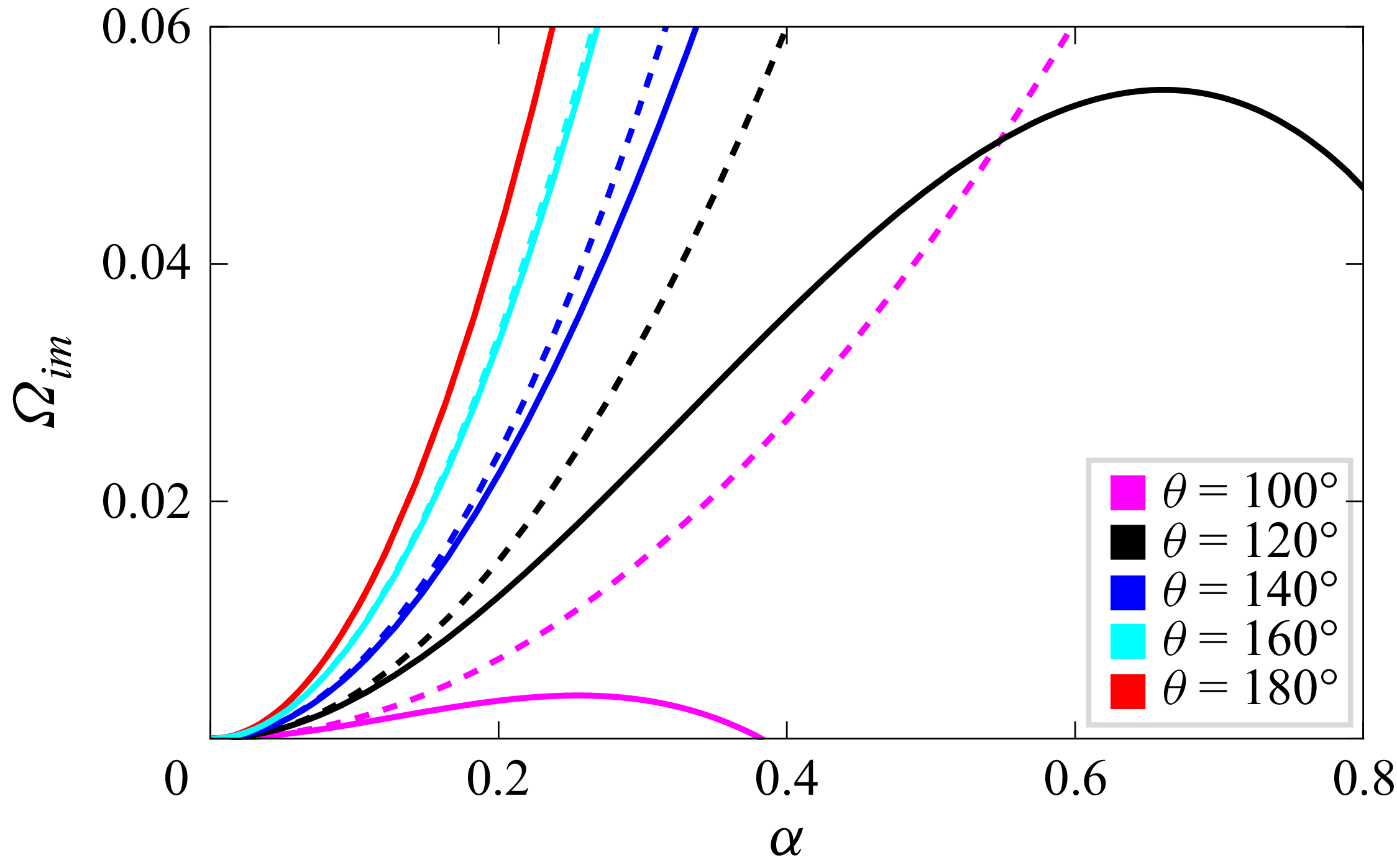
is drawn in figure 7 as a function of
 $\alpha$
for different values of
 $\theta$
. The key result is that the fourth-order analysis shows notable deviations in the growth rate of instability from the third-order analysis and it turns out that the most significant contribution comes from the wave-induced mean flow terms involving Hilbert transform. It is seen from this figure that
 $\varOmega _{\textit{im}}$
obtained from fourth-order results first increases with
 $\alpha$
and then its value decreases, whereas
 $\varOmega _{\textit{im}}$
obtained from third-order results increases steadily with
 $\alpha$
. It is important to note that the fourth-order terms involving Hilbert transform vanish for
 $\theta =180^{\circ }$
and so for this value of
 $\theta$
, there is no fourth-order contribution in the expression of
 $\varOmega _{\textit{im}}$
. Moreover, it is observed from figure 7 that for the same value of
 $\theta$
,
 $\varOmega _{\textit{im}}$
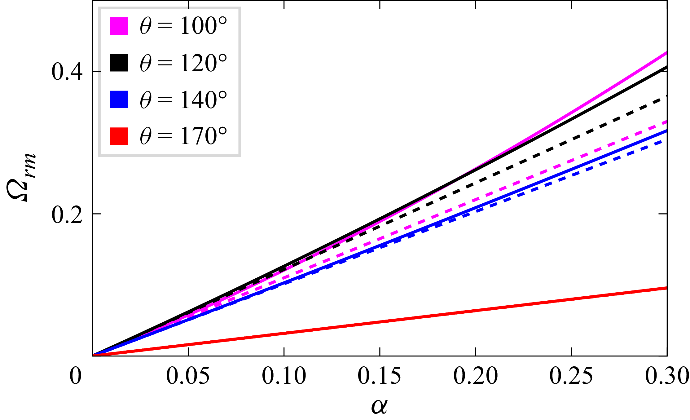
is much smaller for capillary wavetrains than that for gravity wavetrains (see Dhar & Das Reference Dhar and Das1991). In figure 8, the frequency separation of the fastest growing sideband component
 $\varOmega _{\textit{rm}}$
represented by (3.16) is plotted against
 $\alpha$
for several values of
 $\theta$
. Herein, the dashed line corresponds to third-order results and the solid line corresponds to fourth-order results. This figure suggests that
 $\varOmega _{\textit{rm}}$
enhances with the increase of wave steepness
 $\alpha$
.
Plot of maximum growth rate of instability
 $\varOmega _{\textit{im}}$
as a function of
 $\alpha$
for several values of
 $\theta$
. Third-order result (dashed line) and fourth-order result (solid line).

Plot of
 $\varOmega _{\textit{rm}}$
as a function of
 $\alpha$
for several values of
 $\theta$
. Third-order result (dashed line) and fourth-order result (solid line).

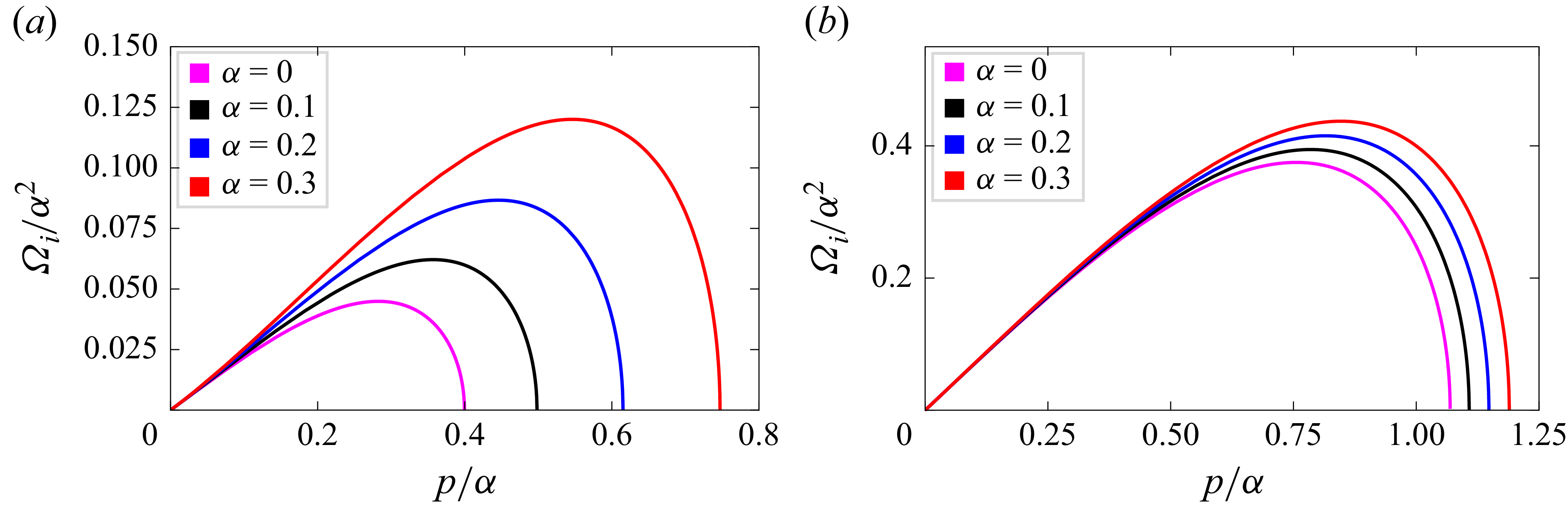
The growth rate
 $\varOmega _i/\alpha ^2$
of the perturbations given by (3.10) as a function of the normalised perturbed wavenumber
 $p/\alpha$
for some values of the wave steepness
 $\alpha$
and angle
 $\theta$
is shown in figure 9. Note that the curve
 $\alpha =0$
corresponds to the ordinary (cubic) nonlinear Schrödinger result. To notice the effect of the wave-induced current more clearly, we have drawn for comparison the growth rate curve of the ordinary nonlinear Schrödinger equations. One can observe that the growth rate of instability increases with the increase of the wave steepness
 $\alpha$
as well as an angle
 $\theta$
.
Plot of
 $\varOmega _i/\alpha ^2$
as a function of
 $p/\alpha$
for various values of
 $\alpha$
.
 $\,(a)\,\theta =90^{\circ }$
;
 $\,(b)\,\theta =120^{\circ }$
.

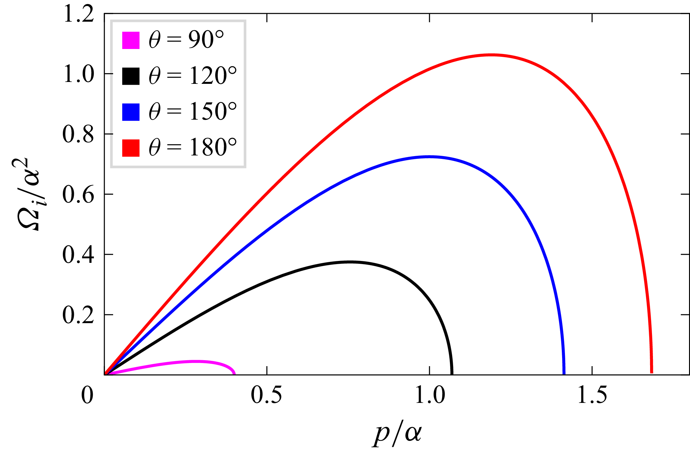
Figure 10 shows the behaviour of the growth rate of instability
 $\varOmega _i/\alpha ^2$
given by (3.17) as a function of
 $p/\alpha$
for several values of
 $\theta$
. A similar trend is observed from this figure as that of figure 4, as the effect of
 $\theta$
on the growth rate. For
 $\theta =0,\,\beta _{12}=0$
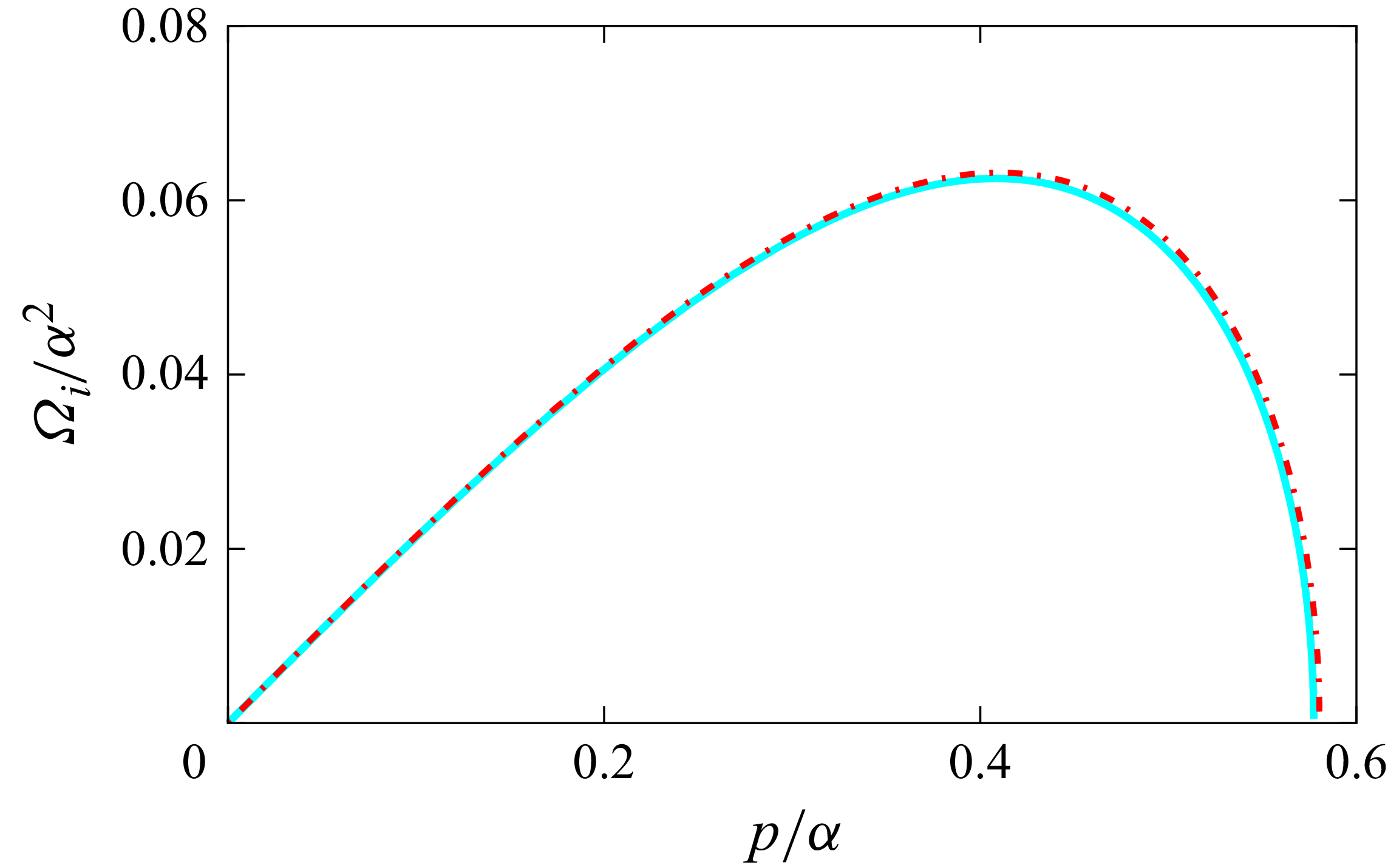
, we have drawn in figure 11 the growth rate
 $\varOmega _i/\alpha ^2$
as a function of
 $p/\alpha$
for a single wavetrain in deep water. As a check, the result we obtained is compared with that obtained by Kharif et al. (Reference Kharif, Abid, Chen and Hsu2025) in their figure 7 and Tiron & Choi (Reference Tiron and Choi2012) in their figure 10(b). In that way, we can verify that these two limiting cases (our results and the result of Kharif et al. (Reference Kharif, Abid, Chen and Hsu2025)) are reproduced exactly, as shown in cyan colour. It is found from this figure that our results agree fairly well with the exact results of Tiron & Choi (Reference Tiron and Choi2012) for wave steepness
 $a_0k=0.32$
, as shown in red colour.
Plot of
 $\varOmega _i/\alpha ^2$
as a function of
 $p/\alpha$
for several values of
 $\theta$
.

Plot of dimensionless growth rate
 $\varOmega _i/\alpha ^2$
for a single wavetrain on deep water as a function of
 $p/\alpha$
when
 $\theta =0$
. Cyan colour represents the analytical results and red colour represents the Tiron & Choi (Reference Tiron and Choi2012) exact results.

3.2. Stability analysis to both longitudinal and transverse perturbations
In this subsection, we perform the stability analysis of the capillary Stokes wavetrains when modulations transverse to the wave propagation direction are also allowed. Instability of a planar wave, appearing due to the interplay between dispersive and nonlinear effects called Benjamin–Feir instability, which has been in continuous focus for several years. Note that the inclusion of transverse modulation requires the consideration of the instability properties of the general Stokes wavetrains within the full form of the NLE equations given by (3.21) and (3.22).
After some algebra, a straight-forward two-dimensional extension of the NLE equations for multiphase wavetrains is given by
 \begin{align} & i\frac {\partial \eta _1}{\partial \tau }+\gamma _1\frac {\partial ^2\eta _1}{\partial X^2}+\delta _1\frac {\partial ^2\eta _1}{\partial Y^2}+i\gamma _2\frac {\partial ^3\eta _1}{\partial X^3}+i\delta _2\frac {\partial ^3\eta _1}{\partial X \partial Y^2}=\big(\beta _{11}\lvert \eta _1\rvert ^2+\beta _{12}\lvert \eta _2\rvert ^2\big)\eta _1 \nonumber \\&\quad +i\big(\lambda _{1}\lvert \eta _1\rvert ^2+\lambda _{2}\lvert \eta _2\rvert ^2\big)\frac {\partial \eta _1}{\partial X}+i\lambda _3\eta ^2_1\frac {\partial \eta ^*_1}{\partial X} +i\lambda _4\eta _1\eta ^*_2\frac {\partial \eta _2}{\partial X}+i\lambda _5\eta _1\eta _2\frac {\partial \eta ^*_2}{\partial X} \nonumber \\&\quad +\varLambda \eta _1 H\left [\frac {\partial }{\partial X}\big(\lvert \eta _1\rvert ^2+\lvert \eta _2\rvert ^2 \big)\right ]\! ,\end{align}
 \begin{align} & i\frac {\partial \eta _2}{\partial \tau }+\gamma _1\frac {\partial ^2\eta _2}{\partial X^2}+\delta _1\frac {\partial ^2\eta _2}{\partial Y^2}+i\gamma _2\frac {\partial ^3\eta _2}{\partial X^3}+i\delta _2\frac {\partial ^3\eta _2}{\partial X \partial Y^2}=\big(\beta _{12}\lvert \eta _1\rvert ^2+\beta _{11}\lvert \eta _2\rvert ^2\big)\eta _2 \nonumber \\&\quad +i\big(\lambda _{1}\lvert \eta _2\rvert ^2+\lambda _{2}\lvert \eta _1\rvert ^2\big)\frac {\partial \eta _2}{\partial X}+i\lambda _3\eta ^2_2\frac {\partial \eta ^*_2}{\partial X}+i\lambda _4\eta _2\eta ^*_1\frac {\partial \eta _1}{\partial X}+i\lambda _5\eta _1\eta _2\frac {\partial \eta ^*_1}{\partial X} \nonumber \\&\quad +\varLambda \eta _2 H\left [\frac {\partial }{\partial X}\big(\lvert \eta _1\rvert ^2+\lvert \eta _2\rvert ^2\big)\right ]\!, \end{align}
where
 $Y=\epsilon y$
and the new derived coefficients
 $\delta _1$
,
 $\delta _2$
are given by
 $\delta _1= {3(2-\cos ^2{(\theta /2))}}/{4}$
,
 $\delta _2= {3}/{8}\cos ^3{(\theta /2)}$
.
Here,
 $H$
is the two-dimensional Hilbert transform operator defined by
 \begin{align} H[\psi (X,Y)]=\frac {1}{2\pi } \int _{-\infty }^\infty \int _{-\infty }^\infty \frac {(X^{\prime }-X)\psi (X^{\prime },Y^{\prime })}{[(X^{\prime }-X)^2+(Y^{\prime }-Y)^2]^{3/2}}\,{{\rm d}}X^{\prime }\,{\rm d}Y^{\prime } .\end{align}
If
 $\psi (X,Y)$
is independent of
 $Y$
,
 $ H[\psi (X)]$
becomes the following after integrating over
 $Y^{\prime }$
:
 \begin{align} H[\psi (X)] = \frac {1}{\pi } P \int _{-\infty }^\infty \frac {\psi (X^{\prime })}{X^{\prime }-X}\,{\rm d}X^{\prime }, \end{align}
where
 $P$
means the principal value of the integral.
If we replace
 $\eta _1$
by
 $\eta _1/2$
and
 $\eta _2$
by
 ${\eta _{2}}/2$
in the NLE equations (3.21) and (3.22), then for
 $\theta =0$
and without second wavetrain, the coupled equations reduce to a single equation which becomes the same as (2.21) of Hogan (Reference Hogan1985). Dysthe (Reference Dysthe1979) has shown specifically that as far as stability characteristics are concerned, it is sufficient to deal with the shortened version of (3.21) and (3.22). The remaining terms, corresponding to setting
 $\gamma _2$
,
 $\delta _2$
,
 $\lambda _i\,(i=1,2,3,4,5)$
to zero, are, however, important in other aspects of wavetrain propagation, as pointed out by Lo & Mei (Reference Lo and Mei1985). Notice that among the new terms due to the fourth-order equations, only the last term involving Hilbert transform contributes to the stability results.
Equations (3.21) and (3.22) admit the uniform Stokes solution given by (3.1). To study the modulational instability, we introduce the following perturbations on these wavetrains:
 \begin{align} \begin{aligned} & \eta _1=\eta _1^{(0)}[1+\tilde \eta _1(X,Y,\tau )], \\ &\eta _2=\eta _2^{(0)}[1+\tilde \eta _2(X,Y,\tau )]. \end{aligned} \end{align}
Substituting (3.25) into (3.21) and (3.22), linearising with respect to
 $\tilde \eta _1$
,
 $\tilde \eta _2$
,
 $\tilde \eta ^*_1$
,
 $\tilde \eta ^*_2$
and then separating the equations after putting
 $\tilde \eta _1=\eta _r^{(1)}+i\eta _i^{(1)},\,\tilde \eta _2=\eta _r^{(2)}+i\eta _i^{(2)}$
, we get the following nonlinear dispersion relation:
 \begin{align} &{\tilde A_1}=- \left [\frac {\alpha ^2(\lambda _1+\lambda _2+\lambda _4)p}{4}\right ]\pm \left [{\tilde A _2}\left \{{\tilde A _2}+\frac {\alpha ^2}{2}\left (\beta _{11}+\beta _{12}-\frac {2\varLambda p^2}{\sqrt {p^2+q^2}}\right )\right \}\right ]^{1/2}, \end{align}
where
 ${\tilde A_1}=\varOmega -c_{\textit{g}}p+\gamma _2p^3+\delta _2pq^2$
,
 ${\tilde A_2}=\gamma _1p^2+\delta _1q^2$
and
 $\varOmega =\tilde \varOmega +c_{\textit{g}}p$
. Here,
 $(p,\,q),\,\varOmega$
denote respectively the perturbed wavevector and frequency.
The calculations are somewhat tedious, but some steps involving Hilbert transform are of interest. The details of derivation are provided in Appendix D.
For instability, we have
 \begin{align} {\tilde A _2}\left \{{\tilde A _2}+\frac {\alpha ^2}{2}\left (\beta _{11}+\beta _{12}-\frac {2\varLambda p^2}{\sqrt {p^2+q^2}}\right )\right \}\lt 0. \end{align}
Note that the overall picture for the onset of the modulational instability is analogous to that occurring in the one-dimensional NLE equations (2.7) and (2.8), though for two-dimensional NLE equations (3.21) and (3.22), the details are different and more intricate with a directional preference and range.
The expression for growth rate of instability
 $\varOmega _{i}$
is given by
 \begin{align} { \varOmega _i}= \left [{\tilde A _2} \left \{{-\tilde A _2}-\frac {\alpha ^2}{2}\left (\beta _{11}+\beta _{12}-\frac {2\varLambda p^2}{\sqrt {p^2+q^2}}\right )\right \}\right ]^{1/2}. \end{align}
For
 $\theta =0$
and
 $\varLambda =0$
and in the absence of a second wavetrain, we recover the expression of the instability growth rate, as obtained by Chen & Saffman (Reference Chen and Saffman1985), given by
 \begin{align} \varOmega _i=\frac {1}{8}\big [3\big(p^2+2q^2\big)\big\{\alpha ^2-3\big(p^2+2q^2\big)\big\}\big ]^{1/2}. \end{align}
For one-dimensional perturbation
 $q=0$
and (3.29) then reduces to
 \begin{align} \varOmega _i=\frac {\sqrt {3}p}{8}\big (\alpha ^2-3p^2\big )^{1/2}. \end{align}
Growth rate of instability
 $\varOmega _i$
attains a maximum value for perturbation wavenumber
 $p=0.0408$
for
 $\alpha =0.1$
and, therefore, the dominant modulational instability of a capillary wavetrain is two-dimensional. By two-dimensional (corresponding to a one-dimensional free surface), we signify that the flow field depends on the single direction of propagation, which will be the
 $x$
-axis. Note that this value of
 $p=0.0408$
is nearly equal to the value obtained by Chen & Saffman (Reference Chen and Saffman1985) (see table 1).
The boundary of the stability region in the perturbed wavevector plane
 $(p,q)$
is given by the following equation:
 \begin{align} {\tilde A _2}+\frac {\alpha ^2}{2}\left (\beta _{11}+\beta _{12}-\frac {2\varLambda p^2}{\sqrt {p^2+q^2}}\right )=0. \end{align}
Figures 12 and 13 show the contour plot of instability growth rate
 $\varOmega _{i}$
given by (3.28) in the
 $(p,q)$
plane for
 $\alpha =0.1,\,0.2$
and several values of
 $\theta$
. It is observed that the growth rate increases with the increase of wave steepness
 $\alpha$
as well as the angle
 $\theta$
. Here, the dot plotted in the figures, located on the
 $p$
axis, corresponds to the maximum growth rate of instability.
Contour plots of the growth rate
 $\varOmega _i(p,q)$
for
 $\alpha =0.1$
and different values of
 $\theta$
. (a)
 $\theta =90^{\circ }$
; (b)
 $\theta =120^{\circ }$
; (c)
 $\theta =150^{\circ }$
. Dots located on the
 $p$
-axis correspond to the maximum growth rate of modulational instability.

Same as figure 12, but
 $\alpha =0.2$
. Dots located on the
 $p$
-axis correspond to the maximum growth rate of modulational instability.

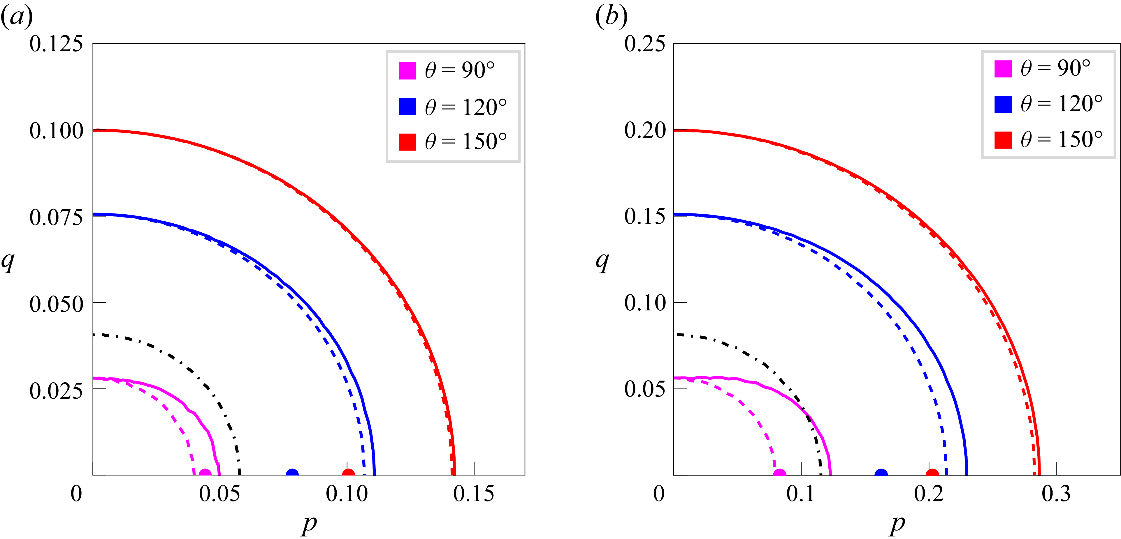
In figure 14, we have plotted the instability diagrams in the
 $(p,q)$
plane for two values of
 $\alpha$
and some values of angle
 $\theta$
. This figure illustrates that the instability region enhances with the increase of
 $\theta$
. Again, the instability region obtained from third-order results diminishes slightly as compared with the fourth-order results. Moreover, one can observe that the domain of instability increases as the wave steepness
 $\alpha$
increases. For a single wavetrain, we have drawn an instability diagram from third-order results which is the same as that obtained by Kharif et al. (Reference Kharif, Abid, Chen and Hsu2025) (see their figure 13), as shown in our figure 14(a) by a dash-dotted line. Therefore, we recover the results of Kharif et al. (Reference Kharif, Abid, Chen and Hsu2025) for a single wavetrain.
Instability diagrams in the
 $(p,q)$
plane for several values of
 $\theta$
.
 $\,(a)\,\alpha =0.1,\,(b)\,\alpha =0.2$
. Third-order result (dashed line), fourth-order result (solid line) and third-order result for a single wavetrain (dash-dotted line). Dots located on the
 $p$
-axis correspond to the maximum growth rate of modulational instability.

Notice that the instability growth rate will be maximum when
 $q=0$
and
 $ {{\rm d}\varOmega _i}/{{\rm d}p}=0$
and the maximum value can be attained for the wavenumber of disturbance
 $p_m$
given by (3.14). We have plotted the dots which are located on the
 $p$
-axis corresponding to the maximum growth rate of instability for three values of
 $\theta$
. Therefore, it can be stated that the dominant modulational instability of weakly nonlinear capillary multiphase wavetrains in deep water is two-dimensional. It is important to mention that for finite amplitude gravity waves, McLean (Reference McLean1982a
,
Reference McLeanb
) has also found that the dominant instability is two-dimensional of Benjamin–Feir type on infinite depth of water, whereas the dominant instability is three-dimensional on water of finite depth.
4. Capillary solitary multiphase wavetrains
It is well known that the nonlinear Schrödinger equation has been shown to be applicable and suggests that solitary envelope wavetrains may exist when the dispersive and nonlinear effects are in balance. In the context of multiphase gravity wavetrains on deep water, it is important to note that the modulational instabilities and solitary wave solutions have been obtained when
 $0\lt \theta \lt 70.5^{\circ }$
may be attributed to self-modulation effects, whereas those have been obtained when
 $136.1^{\circ }\lt \theta \leqslant 180^{\circ }$
may be attributed to self-focusing effects (see Roskes Reference Roskes1976a
).
The third-order NLE equations corresponding to (2.7) and (2.8) are given by
 \begin{align} i\frac {\partial \eta _1}{\partial \tau }+\gamma _1\frac {\partial ^2 \eta _1}{\partial X^2}=\big(\beta _{11}{\lvert \eta _1\rvert }^2+\beta _{12}{\lvert \eta _2\rvert }^2\big)\eta _1, \end{align}
 \begin{align} i\frac {\partial \eta _2}{\partial \tau }+\gamma _1\frac {\partial ^2 \eta _2}{\partial X^2}=\big(\beta _{12}{\lvert \eta _1\rvert }^2+\beta _{11}{\lvert \eta _2\rvert }^2\big)\eta _2 .\end{align}
In the unstable case, we seek the multiphase solitary envelope wavetrain solutions of (4.1) and (4.2) of the following form:
 \begin{align} \begin{aligned} &\eta _1=\eta _{01}\exp (i\theta _1\tau ) {\textrm {sech}}(\delta X), \\ &\eta _2=\eta _{02}\exp (i\theta _2\tau ){\textrm {sech}}(\delta X). \end{aligned} \end{align}
Here, the spread parameter
 $\delta$
is the same for both the modes. We observe that
 $\eta _{01}$
,
 $\eta _{02}$
and
 $\delta$
satisfy the following equation as follows:
 \begin{align} \delta ^2=-\frac {(\beta _{11}+\beta _{12})\left(\eta ^2_{01}+\eta ^2_{02}\right)}{4\gamma _1}. \end{align}
This solitary envelope solution exhibits that energy may be spread to long distances in a concentrated packet of waves, without being demolished by dispersion. Equation (4.4) shows that solitary envelope solution of the above-mentioned form is possible if the condition
 \begin{align} (\beta _{11}+\beta _{12})\gamma _1\lt 0 \end{align}
is satisfied.
An examination of the coefficients
 $\gamma _1, \,\beta _{11},\, \beta _{12}$
and figure 2 demonstrates that the condition (4.5) will be satisfied when
 $86.86^{\circ }\lt \theta \leqslant 180^{\circ }$
. Therefore, we may come to an important conclusion that within the framework of the NLE equation the existence of capillary envelope soliton and modulational instability is concomitant, consistent with the results obtained by Roskes (Reference Roskes1976a
) for gravity wavetrains.
5. Concluding remarks
In this paper, the fourth-order coupled NLE equations for multiphase capillary wavetrains on deep water have been used to study the modulational instability of finite amplitude capillary Stokes wavetrains. We have presented a simple model for the interaction of two capillary wavetrains travelling in different wave directions. It is well known that the fourth-order NLE equation is a good starting point for the study of nonlinear periodic waves on deep water, as first pointed out by Dysthe (Reference Dysthe1979) and later elaborated by Janssen (Reference Janssen1983). As it turns out, the most significant contribution introduced to fourth-order is the mean flow response to non-uniformities in the radiation stress caused by modulation of a finite amplitude wave. Here, we intend to extend the Dysthe (Reference Dysthe1979) approach for multiphase capillary wavetrains and to investigate some interesting properties of modulational instability of weakly nonlinear wavetrains on deep water. We have also made the instability analysis of capillary wavetrains to oblique perturbations. It is important to note that the wave induced mean flow response corresponds to fourth-order terms involving Hilbert transform in (2.7) and (2.8). The effect of these two terms will die out when
 $\theta =180^{\circ }$
and so for this value of
 $\theta$
, there is no fourth-order contribution in the instability properties.
The new findings of this work are as follows. (i) For weakly nonlinear multiphase capillary Stokes wavetrains on deep water, we obtain the instability results, namely, the growth rate, bandwidth, perturbed frequency at marginal stability and the normalised frequency separation of fastest growing sideband component. (ii) The key result is that the fourth-order analysis shows significant deviations in the maximum growth rate of instability when compared with the third-order analysis. (iii) It is found that the cross-interaction nonlinearity is stronger than the self-interaction one when the angle
 $\theta$
lies between
 $0^{\circ }$
and
 $86.86^{\circ }$
. (iv) Given a single unstable plane wavetrain, we show an important feature that the introduction of a second wavetrain, moving in a different direction, can result in an increase of the instability growth rate and enlargement of the domain of instability. (v) A linear stability analysis to transverse perturbations on a liquid layer of infinite depth for capillary waves is presented, showing that the dominant modulational instability of weakly nonlinear capillary wavetrains is two-dimensional on deep water. (vi) Furthermore, we present the stability results for capillary solitary envelopes on infinite depth of water. We exhibit that the existence of capillary envelope soliton and modulational instability is concomitant, compatible with the remark of Roskes (Reference Roskes1976a
) for multiphase gravity wavetrains.
Acknowledgements
This work was commenced during a visit of Professor A. K. Dhar to the National Sun Yat-sen University, Kaohsiung, Taiwan, Department of Marine Environmental Engineering. The authors would like to express gratitude to the anonymous reviewers for their constructive and insightful comments and suggestions in improving the paper.
Funding
A. K. Dhar acknowledges and sincerely thanks the Indian Institute of Engineering Science and Technology (IIEST), Shibpur for providing him the financial support through a CPDA grant (No. CPDA/13/25). The award of Senior Research Fellowship (Ref. No. 163/ACAD/2025) to S. Mukherjee by the IIEST, Shibpur is gratefully recognised.
Declaration of interests
The authors report no conflict of interest.
Appendix A. Derivation of (2.7) and (2.8)
Since the disturbance is considered to be progressive waves, we take the solutions of the (2.1)–(2.4) in the following form:
 \begin{align} &M=M_{00}+\sum _{m=0}^{\infty }\sum _{n=0}^{\infty }\left \{M_{\textit{mn}}\exp i(m\psi _1+n\psi _2)+M^{*}_{\textit{mn}}\exp -i(m\psi _1+n\psi _2)\right \},\nonumber \\ & \qquad \,\, m=n \neq 0, \end{align}
where
 $M$
stands for
 $\varPhi$
and
 $\eta$
and
 $\psi _1=k_{1x}x+k_{1y}y-\sigma _1t,\,\psi _2=k_{2x}x+k_{2y}y-\sigma _2t$
. Herein,
 $\varPhi _{00},\,\varPhi _{\textit{mn}},\,\varPhi ^*_{\textit{mn}}$
are slowly varying functions of
 $z$
,
 $x_1=\epsilon x,\,y_1=\epsilon y,\,t_1=\epsilon t$
;
 $\eta _{00},\,\eta _{\textit{mn}},\,\eta ^*_{\textit{mn}}$
are functions of
 $x_1,\,y_1,\,t_1$
.
 $\text{Asterisk}(*)$
represents the complex conjugate. We introduce the small ordering parameter
 $\epsilon$
, which signifies both the slow modulations and the wave amplitude.
Inserting the expression (A1) in (2.1) and equating the coefficients of
 $\exp i(m\psi _1+n\psi _2)$
for
 $(m,n)=\{(1,0),(0,1),(2,0),(0,2),(1,1),(1,-1)\},$
we find the equations as follows:
 \begin{align} \left [\frac {{\rm d}^2}{{\rm d}z^2}-{\tilde R^2_{\textit{mn}}}\right ] \varPhi _{\textit{mn}}=0, \end{align}
where
 $\tilde R^2_{\textit{mn}}=(mk_{1x}+nk_{2x}-i\epsilon ({\partial }/{\partial x_1}))^2+(mk_{1y}+nk_{2y}-i\epsilon ({\partial }/{\partial y_1}) )^2$
.
In view of (2.4), the solution of (A2) is given by
 \begin{align} \varPhi _{\textit{mn}}=B_{\textit{mn}}\exp (\tilde R_{\textit{mn}}z), \end{align}
in which
 $B_{\textit{mn}}$
for different values of
 $(m,n)$
are functions of
 $x_1,\,y_1$
and
 $t_1$
.
To obtain the solution corresponding to
 $(m,n)=(0,0)$
, it is convenient to take the Fourier transform of
 $\varPhi _{00}$
defined by
 \begin{align} \tilde \varPhi _{00}=\iiint _{-\infty }^{\infty }\varPhi _{00}\exp i(\tilde k_x x_1+\tilde k_y y_1-\tilde \sigma t_1)\,{\rm d}x_1\,{\rm d}y_1\,{\rm d}t_1, \end{align}
where
 $\tilde k^2=\epsilon ^2(\tilde k^2_x +\tilde k^2_y )$
.
The solution of this transformed equation satisfying the boundary condition (2.4) becomes
 \begin{align} \tilde \varPhi _{00}=\tilde B_{00}\exp (\lvert \tilde k\rvert z), \end{align}
in which
 $\tilde B_{00}$
is a function of
 $\tilde k_x,\,\tilde k_y$
and
 $\tilde \sigma$
.
Again, injecting the expression (A1) in the Taylor series expanded forms of (2.2) and (2.3) about
 $z=0$
, and then equating the coefficients of
 $\exp i(m\psi _1+n\psi _2)$
for
 $(m,n)=\{(1,0),(0,1),(2,0),(0,2),(1,1),(1,-1),(0,0)\}$
on both sides, we find the seven sets of equations in each of which we insert the solutions for
 $\varPhi _{\textit{mn}}$
given by (A3) and (A5). To solve these sets of equations, we consider the perturbation expansions given by
 \begin{align} &N_{\textit{mn}}=\sum _{r=1}^{\infty }\epsilon ^rN_{\textit{mnr}},\qquad \qquad (m,n)=\{(1,0),(0,1)\},\nonumber \\ &N_{\textit{mn}}=\sum _{r=2}^{\infty }\epsilon ^rN_{\textit{mnr}},\qquad \qquad (m,n)=\{(2,0),(0,2),(1,1),(1,-1),(0,0)\}, \end{align}
where
 $N_{\textit{mn}}$
means
 $B_{\textit{mn}}$
and
 $\eta _{\textit{mn}}$
.
Inserting the expansions (A6) in the seven sets of equations and then equating the coefficients of different powers of
 $\epsilon$
on both sides, we find a sequence of equations. Finally, eliminating
 $B_{10}$
or
 $B_{01}$
from the two equations corresponding to
 $(m,n)=(1,0)\,\text{or}\,(0,1)$
, we get the following two equations:
 \begin{align} & \left \{\sum {^2}-\tilde R_{10}\right \}\eta _{10}=-i\sum a_{10}-\tilde R_{10}b_{10}, \end{align}
 \begin{align} & \left \{\sum {^2}-\tilde R_{01}\right \}\eta _{01}=-i\sum a_{01}-\tilde R_{01}b_{01}, \end{align}
where
 $\sum =(\sigma +i\epsilon ({\partial }/{\partial t_1}) )$
and
 $a_{10},\,a_{01},\,b_{10},\,b_{01}$
represent the nonlinear expressions in terms of
 $\eta _{10}$
and
 $\,\eta _{01}$
.
Taking
 $\eta _{1}=\eta _{101}+\epsilon \eta _{102}$
and
 $\eta _2=\eta _{011}+\epsilon \eta _{012}$
, we obtain the two fourth-order coupled NLE equations given by (2.7) and (2.8).
Appendix B. Detailed calculation of the coefficients
 $\beta _{12}$
and
$\gamma _1$
when
$\kappa =Tk^2/g\rightarrow \infty$


Put
 $\kappa =1/\tilde \kappa$
in the expressions of
 $\beta _{12}$
and
 $\gamma _1$
so that when
 $\kappa \rightarrow \infty$
, we have
 $\tilde \kappa =0$
,
 \begin{align} \beta _{12}& =\dfrac {2}{\Delta }\cos \dfrac {\theta }{2} \left(1-2 \cos \dfrac {\theta }{2}\right)\Biggl [(1+\kappa )\left(1+\sin ^2\dfrac {\theta }{2}\right)-\cos ^2\dfrac {\theta }{2}\left (1+4\kappa \cos ^2\dfrac {\theta }{2}\right )\Biggr ]\nonumber \\&\quad -2(1+\kappa )\sin ^2\dfrac {\theta }{2}\left [\dfrac {\sin ^2\dfrac {\theta }{2}}{1+4\kappa \sin ^2\dfrac {\theta }{2}}-\dfrac {1}{\Delta }\left \{\cos \dfrac {\theta }{2}\left(1+\sin ^2\dfrac {\theta }{2} \right) -2\cos ^2\dfrac {\theta }{2}\right \}\right ] \nonumber \\& \quad -\dfrac {\kappa }{2(1+\kappa )}\big(\sin ^2\theta +3\cos ^2\theta \big)+3\cos \theta +1\nonumber \\& =\dfrac {2\tilde \kappa }{(1+\tilde \kappa )\bigl(2-\cos \dfrac {\theta }{2}\bigr)}\cos \dfrac {\theta }{2} \Bigl (\!1-2 \cos \dfrac {\theta }{2}\Bigr )\Biggl [\!\dfrac {(1\!+\tilde \kappa )}{\tilde \kappa }\Bigl (\!1\!+\sin ^2\dfrac {\theta }{2}\Bigr )-\dfrac {\cos ^2\dfrac {\theta }{2}}{\tilde \kappa }\left (\tilde \kappa \!+4\cos ^2\dfrac {\theta }{2}\right )\!\Biggr ]\nonumber \\& \quad -\dfrac {2(1+\tilde \kappa )}{\tilde \kappa }\sin ^2\dfrac {\theta }{2} \!\left [ \!\dfrac {\tilde \kappa \sin ^2\dfrac {\theta }{2}}{\tilde \kappa +4\sin ^2\dfrac {\theta }{2}}-\dfrac {\tilde \kappa }{(1+\tilde \kappa )(2-\cos \dfrac {\theta }{2})}\left \{\cos \dfrac {\theta }{2} \!\left(\!1+\sin ^2\dfrac {\theta }{2} \!\right) \! -2\cos ^2\dfrac {\theta }{2} \!\right \} \!\!\right ] \nonumber \\& \quad -\dfrac {1}{2(1+\tilde \kappa )}\bigl(\sin ^2\theta +3\cos ^2\theta \bigr)+3\cos \theta +1\nonumber \\& =\dfrac {2}{(2-\cos \dfrac {\theta }{2})}\cos \dfrac {\theta }{2} \left(1-2 \cos \dfrac {\theta }{2}\right)\left [2-\cos ^2\dfrac {\theta }{2}-4\cos ^4\dfrac {\theta }{2}\right ]\nonumber \\& \quad -2\sin ^2\dfrac {\theta }{2}\left [\dfrac {1}{4}-\dfrac {1}{\bigl(2-\cos \dfrac {\theta }{2}\bigr)}\left \{\cos \dfrac {\theta }{2}\left(2-\cos ^2\dfrac {\theta }{2}\right) -2\cos ^2\dfrac {\theta }{2}\right \}\right ] \nonumber \\& \quad -\dfrac {1}{2}(\sin ^2\theta +3\cos ^2\theta )+3\cos \theta +1\qquad (\text{as}\,\,\tilde \kappa =0)\nonumber \\& =\dfrac {2\cos \dfrac {\theta }{2}}{(2-\cos \dfrac {\theta }{2})} \Biggl [\left(1-2 \cos \dfrac {\theta }{2}\right)\Biggl (2-\cos ^2\dfrac {\theta }{2}-4\cos ^4\dfrac {\theta }{2}\Biggr )\nonumber \\& \quad +{\left (1-\cos ^2\dfrac {\theta }{2}\right )}\Bigl (2-\cos ^2\dfrac {\theta }{2} -2\cos \dfrac {\theta }{2}\Bigr )\Biggr ]-\dfrac {1}{2}\left (1-\cos ^2\dfrac {\theta }{2}\right ) \nonumber \\& \quad -\dfrac {1}{2}(1+2\cos ^2\theta )+3\cos \theta +1 \nonumber \\& =\dfrac {2\cos \dfrac {\theta }{2}\left(4-6\cos \dfrac {\theta }{2}-4\cos ^2\dfrac {\theta }{2}+4\cos ^3\dfrac {\theta }{2}-3\cos ^4\dfrac {\theta }{2}+8\cos ^5\dfrac {\theta }{2}\right)}{ \left(2-\cos \dfrac {\theta }{2} \right)}\nonumber\\& \quad+\dfrac {21}{2}\cos ^2\dfrac {\theta }{2}-4\cos ^4\dfrac {\theta }{2}-4 \nonumber \\ \gamma _1 & = \dfrac {1}{4(1+\kappa )}\Bigg [3\kappa \left (1+\cos ^2\dfrac {\theta }{2}\right )+\sin ^2\dfrac {\theta }{2}\Biggr ]-\dfrac {(1+3\kappa )^2}{8(1+\kappa )^2}\cos ^2\dfrac {\theta }{2}\nonumber \\ &=\dfrac {1}{4(1+\tilde \kappa )}\Bigg [3\left (1+\cos ^2\dfrac {\theta }{2}\right )+\tilde \kappa \sin ^2\dfrac {\theta }{2}\Biggr ]-\dfrac {(\tilde \kappa +3)^2}{8(1+\tilde \kappa )^2}\cos ^2\dfrac {\theta }{2}\nonumber \\ &=\dfrac {3\left(2-\cos ^2\dfrac {\theta }{2}\right)}{8}, \end{align}
 \begin{align} \text{where}\,\varDelta &=\frac {1}{2}\big [(\sigma _1+\sigma _2)^2-\lvert k_1+k_1\rvert (1+\kappa )\big ]\nonumber \\& =\frac {1}{2}\Bigl [4\sigma ^2- 2k\cos \frac {\theta }{2}(1+\kappa )\Bigr ]\nonumber \\& =2(1+\kappa )-\cos \frac {\theta }{2}(1+\kappa )\nonumber \\& =(1+\kappa )\left(2-\cos \frac {\theta }{2} \right)\nonumber \\& =\frac {(1+\tilde \kappa )}{\tilde \kappa } \left(2-\cos \frac {\theta }{2}\right). \end{align}
Appendix C. Coefficients appearing in (2.7) and (2.8) have the following definitions
 \begin{align} \gamma _1&=\dfrac {3\left(2-\cos ^2\dfrac {\theta }{2}\right)}{8},\quad \gamma _2=\dfrac {\cos \dfrac {\theta }{2}\left(2-\cos ^2\dfrac {\theta }{2}\right)}{16} ,\quad \beta _{11}=-\dfrac {1}{4} \nonumber \\\beta _{12}&=\dfrac {2\cos \dfrac {\theta }{2}\left(4-6\cos \dfrac {\theta }{2}-4\cos ^2\dfrac {\theta }{2}+4\cos ^3\dfrac {\theta }{2}-3\cos ^4\dfrac {\theta }{2}+8\cos ^5\dfrac {\theta }{2}\right)}{\left(2-\cos \dfrac {\theta }{2}\right)}\nonumber \\&\quad+\dfrac {21}{2}\cos ^2\dfrac {\theta }{2}-4\cos ^4\dfrac {\theta }{2}-4 \nonumber \\\lambda _{1}&=\dfrac {3}{4}\cos \dfrac {\theta }{2} \nonumber \\\lambda _{2}&=\dfrac {\left(1-2\cos \dfrac {\theta }{2}-2\cos ^2\dfrac {\theta }{2}\right)}{2\left(2-\cos \dfrac {\theta }{2}\right)}\left \{\dfrac {3\cos \dfrac {\theta }{2}\left(1-2\cos \dfrac {\theta }{2}\right)\!\left(2-\cos \dfrac {\theta }{2}-\cos ^2\dfrac {\theta }{2}\right)}{\left(2-\cos \dfrac {\theta }{2}\right)}-2 \right. \nonumber \\& \left. \quad +4\cos \dfrac {\theta }{2} -\cos ^2\dfrac {\theta }{2}+3\cos ^3\dfrac {\theta }{2}+\cos ^4\dfrac {\theta }{2} \vphantom{\dfrac {3\cos \dfrac {\theta }{2}\left(1-2\cos \dfrac {\theta }{2}\right)\!\left(2-\cos \dfrac {\theta }{2}-\cos ^2\dfrac {\theta }{2}\right)}{\left(2-\cos \dfrac {\theta }{2}\right)}}\right \} \nonumber \\ & \quad -\dfrac {\cos \dfrac {\theta }{2}\left(3\cos \dfrac {\theta }{2}+4\right)\!\left(2-\cos \dfrac {\theta }{2}-\cos ^2\dfrac {\theta }{2}\right)}{2\left(2-\cos \dfrac {\theta }{2}\right)}\nonumber \nonumber \\&\quad +\dfrac {7\cos \dfrac {\theta }{2}+2\cos ^2\dfrac {\theta }{2}-6\cos ^3\dfrac {\theta }{2}+4\cos ^4\dfrac {\theta }{2}+64\cos ^5\dfrac {\theta }{2}}{8}\nonumber \nonumber \\\lambda _{3}&=-\dfrac {1}{8}\cos \dfrac {\theta }{2}, \end{align}
 \begin{align} \lambda _{4}&=\dfrac {\left(1-2\cos \dfrac {\theta }{2}-2\cos ^2\dfrac {\theta }{2}\right)}{2\left(2-\cos \dfrac {\theta }{2}\right)}\left \{\dfrac {3\cos \dfrac {\theta }{2}\left(1-2\cos \dfrac {\theta }{2}\right)\!\left(2-\cos \dfrac {\theta }{2}-\cos ^2\dfrac {\theta }{2}\right)}{\left(2-\cos \dfrac {\theta }{2}\right)}-2 \right. \nonumber \\& \left. \quad +4\cos \dfrac {\theta }{2} -\cos ^2\dfrac {\theta }{2}+3\cos ^3\dfrac {\theta }{2}+\cos ^4\dfrac {\theta }{2} \vphantom{\dfrac {3\cos \dfrac {\theta }{2}\left(1-2\cos \dfrac {\theta }{2}\right)\!\left(2-\cos \dfrac {\theta }{2}-\cos ^2\dfrac {\theta }{2}\right)}{\left(2-\cos \dfrac {\theta }{2}\right)}}\right \} \nonumber \\& -\dfrac {\cos \dfrac {\theta }{2}\left(\cos ^2\dfrac {\theta }{2}\!+\!2\cos \dfrac {\theta }{2}\!+4\right)\!\left(2-\cos \dfrac {\theta }{2}-\cos ^2\dfrac {\theta }{2}\right)}{2\left(2-\cos \dfrac {\theta }{2}\right)}\nonumber \nonumber \\&\quad +\dfrac {-81\cos \dfrac {\theta }{2}+10\cos ^2\dfrac {\theta }{2}+2\cos ^3\dfrac {\theta }{2}-20\cos ^4\dfrac {\theta }{2}+64\cos ^5\dfrac {\theta }{2}}{8} \nonumber \\&\quad+ \cos \dfrac {\theta }{2}(\cos ^2\theta +4\cos \theta +3) \nonumber \\\lambda _5&=\dfrac {\cos \dfrac {\theta }{2}}{8}\left \{48\cos \dfrac {\theta }{2}-2\cos ^2\dfrac {\theta }{2}\Bigl (5+12\sin \dfrac {\theta }{2}\Bigr )-\Bigl (9-2\sin \dfrac {\theta }{2}+16\sin ^2\dfrac {\theta }{2}\Bigr )\right \}\nonumber \nonumber \\&\quad -\dfrac {\left(2-2\cos \dfrac {\theta }{2}-\cos ^2\dfrac {\theta }{2}\right)\cos \dfrac {\theta }{2}}{2(2-\cos \dfrac {\theta }{2})}\left \{12+5\cos \dfrac {\theta }{2}+12\cos ^3\dfrac {\theta }{2}\right \} \nonumber \\\varLambda &=2\cos ^2\dfrac {\theta }{2}. \end{align}
Appendix D. Derivation of nonlinear dispersion relation
Inserting (3.25) into (3.21) and (3.22), and linearising with respect to
 $\eta _r^{(1)},\,\eta _i^{(1)},\,\eta _r^{(2)},\,\eta _i^{(2)}$
, we obtain the four equations as follows:
 \begin{align} & -\frac {\partial \eta _i^{(1)}}{\partial \tau }+\gamma _1\frac {\partial ^2\eta {_r}^{(1)}}{\partial X^2}+\delta _1\frac {\partial ^2\eta _r^{(1)}}{\partial Y^2}-\gamma _2 \frac {\partial ^3\eta _i^{(1)}} {\partial X^3}-\delta _2\frac {\partial ^3\eta _i^{(1)}} {\partial X \partial Y^2}-\frac {\beta _{11}}{2}\eta ^2_{01}\eta _r^{(1)} \nonumber \\[5pt]& -\frac {\beta _{12}}{2}\eta ^2_{02}\eta _r^{(2)} +\frac {1}{4}\left\{(\lambda _1-\lambda _3)\eta ^2_{01}+\lambda _2\eta ^2_{02}\right\}\frac {\partial \eta _i^{(1)}}{\partial X}+\frac {1}{4}(\lambda _4-\lambda _5)\eta ^2_{02}\frac {\partial \eta _i^{(2)}}{\partial X}\nonumber \\[5pt]&-\frac {\varLambda }{4\pi }\Biggl [\eta ^2_{01} \int _{-\infty }^\infty \int _{-\infty }^\infty \frac {(X^{\prime }-X){\rm d}X^{\prime }{\rm d}Y^{\prime }}{[(X^{\prime }-X)^2+(Y^{\prime }-Y)^2]^{3/2}}\frac {\partial \eta _r^{(1)}}{\partial X'}\ \nonumber \\[5pt]& +\eta ^2_{02} \int _{-\infty }^\infty \int _{-\infty }^\infty \frac {(X^{\prime }-X)\,{\rm d}X^{\prime }\,{\rm d}Y^{\prime }}{[(X^{\prime }-X)^2+(Y^{\prime }-Y)^2]^{3/2}}\frac {\partial \eta _r^{(2)}}{\partial X'}\Biggr ]=0, \\[-10pt] \nonumber \end{align}
 \begin{align} &\frac {\partial \eta _r^{(1)}}{\partial \tau }+\gamma _1\frac {\partial ^2\eta {_i}^{(1)}}{\partial X^2}+\delta _1\frac {\partial ^2\eta _i^{(1)}}{\partial Y^2}+\gamma _2 \frac {\partial ^3\eta _r^{(1)}} {\partial X^3}+\delta _2\frac {\partial ^3\eta _r^{(1)}} {\partial X \partial Y^2} \nonumber \\& -\frac {1}{4}\Bigl \{(\lambda _1+\lambda _3)\eta ^2_{01}+\lambda _2\eta ^2_{02}\Bigr \}\frac {\partial \eta _r^{(1)}}{\partial X} -\frac {1}{4}(\lambda _4+\lambda _5)\eta ^2_{02}\frac {\partial \eta _r^{(2)}}{\partial X}=0, \\[-12pt] \nonumber \end{align}
 \begin{align} & -\frac {\partial \eta _i^{(2)}}{\partial \tau }+\gamma _1\frac {\partial ^2\eta {_r}^{(2)}}{\partial X^2}+\delta _1\frac {\partial ^2\eta _r^{(2)}}{\partial Y^2}-\gamma _2 \frac {\partial ^3\eta _i^{(2)}} {\partial X^3}-\delta _2\frac {\partial ^3\eta _i^{(2)}} {\partial X \partial Y^2}-\frac {\beta _{11}}{2}\eta ^2_{02}\eta _r^{(2)}-\frac {\beta _{12}}{2}\eta ^2_{01}\eta _r^{(1)}\nonumber \\ &+\frac {1}{4}\{(\lambda _1-\lambda _3)\eta ^2_{02}+\lambda _2\eta ^2_{01}\}\frac {\partial \eta _i^{(2)}}{\partial X} +\frac {1}{4}(\lambda _4-\lambda _5)\eta ^2_{01}\frac {\partial \eta _i^{(1)}}{\partial X}\nonumber \\ &-\frac {\varLambda }{4\pi }\Biggl [\eta ^2_{01} \int _{-\infty }^\infty \int _{-\infty }^\infty \frac {(X^{\prime }-X)\,{\rm d}X^{\prime }\,{\rm d}Y^{\prime }}{[(X^{\prime }-X)^2+(Y^{\prime }-Y)^2]^{3/2}}\frac {\partial \eta _r^{(1)}}{\partial X'}\nonumber \\ & +\eta ^2_{02} \int _{-\infty }^\infty \int _{-\infty }^\infty \frac {(X^{\prime }-X)\,{\rm d}X^{\prime }\,{\rm d}Y^{\prime }}{[(X^{\prime }-X)^2+(Y^{\prime }-Y)^2]^{3/2}}\frac {\partial \eta _r^{(2)}}{\partial X'}\Biggr ]=0, \\[-12pt] \nonumber \end{align}
 \begin{align} &\frac {\partial \eta _r^{(2)}}{\partial \tau }+\gamma _1\frac {\partial ^2\eta {_i}^{(2)}}{\partial X^2}+\delta _1\frac {\partial ^2\eta _i^{(2)}}{\partial Y^2}+\gamma _2 \frac {\partial ^3\eta _r^{(2)}} {\partial X^3}+\delta _2\frac {\partial ^3\eta _r^{(2)}} {\partial X \partial Y^2} \nonumber \\ & -\frac {1}{4}\Bigl \{(\lambda _1+\lambda _3)\eta ^2_{02}+\lambda _2\eta ^2_{01}\Bigr \}\frac {\partial \eta _r^{(2)}}{\partial X} -\frac {1}{4}(\lambda _4+\lambda _5)\eta ^2_{01}\frac {\partial \eta _r^{(1)}}{\partial X}=0 . \\[9pt] \nonumber \end{align}
We now suppose the time dependence of
 $\eta _{r}^{(1)},\,\eta _{i}^{(1)},\,\eta _{r}^{(2)},\,\eta _{i}^{(2)}$
to be of the form
 $\exp (-i\tilde \varOmega \tau )$
. Next, taking the Fourier transform of (D1)–(D4) with respect to
 $X,\,Y$
defined by
 \begin{align} (\hat \eta _{r}^{(1)},\,\hat \eta _{i}^{(1)},\,\hat \eta _{r}^{(2)},\,\hat \eta _{i}^{(2)}) =\frac {1}{2\pi } \int _{-\infty }^\infty \int _{-\infty }^\infty (\eta _{r}^{(1)},\,\eta _{i}^{(1)},\,\eta _{r}^{(2)},\,\eta _{i}^{(2)})\exp -i(pX+qY)\,{\rm d}X\,{\rm d}Y, \end{align}
we get the following equations:
 \begin{align} \textit{iP} \hat \eta _{i}^{(1)}-Q\hat \eta _{r}^{(1)}+ip\frac {(\lambda _4-\lambda _5)}{4} \alpha ^2\hat \eta _{i}^{(2)}-R\hat \eta _{r}^{(2)}=0, \end{align}
 \begin{align} \big(\gamma _1 p^2+\delta _1 q^2 \big)\hat \eta _{i}^{(1)}+iS\hat \eta _{r}^{(1)}+i\frac {(\lambda _4+\lambda _5)}{4} \alpha ^{2} p\hat \eta _{r}^{(2)}=0, \end{align}
 \begin{align} \textit{iP} \hat \eta _{i}^{(2)}-Q\hat \eta _{r}^{(2)}+ip\frac {(\lambda _4-\lambda _5)}{4} \alpha ^2\hat \eta _{i}^{(1)}-R\hat \eta _{r}^{(1)}=0 ,\end{align}
 \begin{align} \big(\gamma _1 p^2+\delta _1 q^2 \big)\hat \eta _{i}^{(2)}+iS\hat \eta _{r}^{(2)}+i\frac {(\lambda _4+\lambda _5)}{4} \alpha ^{2} p\hat \eta _{r}^{(1)}=0, \\[9pt] \nonumber \end{align}
where
 $P=\tilde \varOmega +\gamma _2p^3+\delta _2 p q^3+\frac {1}{4}(\lambda _1+\lambda _2-\lambda _3)\alpha ^2p$
,
 $Q=\gamma _1p^2+\delta _1 q^2+ {\alpha ^2}/{2}\Bigl (\beta _{11}- {\varLambda p^2}/{\sqrt {p^2+q^2}}\Bigr )$
,
 $R=\frac {\alpha ^2}{2}(\beta _{12}- {\varLambda p^2}/{\sqrt {p^2+q^2}})$
,
 $S=\tilde \varOmega +\gamma _2p^3+\delta _2 p q^3+\frac {1}{4}(\lambda _1+\lambda _2+\lambda _3)\alpha ^2p$
and
 $p,\,q$
are the longitudinal and transverse wavenumbers of perturbation.
Adding (D6), (D8) and (D7), (D9), we have
 \begin{align} i \left\{P+\frac {1}{4}(\lambda _4-\lambda _5)\alpha ^2p \right\}\Bigl \{\hat \eta _{i}^{(1)}+\hat \eta _{i}^{(2)}\Bigr \}-(Q+R)\Bigl \{\hat \eta _{r}^{(1)}+\hat \eta _{r}^{(2)}\Bigr \}=0, \\[-10pt] \nonumber \end{align}
 \begin{align} \big(\gamma _1p^2+\delta _1q^2 \big)\Bigl \{\hat \eta _{i}^{(1)}+\hat \eta _{i}^{(2)}\Bigr \}+ i\Bigl \{S+\frac {1}{4}(\lambda _4+\lambda _5)\alpha ^2p\Bigr \}\Bigl \{\hat \eta _{r}^{(1)}+\hat \eta _{r}^{(2)}\Bigr \}=0. \\[9pt] \nonumber \end{align}
For a non-trivial solution of (D10) and (D11) to exist, the determinant of these equations is zero and this gives the following nonlinear dispersion relation, where it is assumed that the amplitudes of the two modes are equal, that is,
 $\eta _{01}=\eta _{02}=\alpha$
:
 \begin{align} &\Biggl [\big(\tilde \varOmega +\gamma _2p^3+\delta _2pq^2 \big)+\frac {(\lambda _1+\lambda _2-\lambda _3+\lambda _4-\lambda _5)}{4}\alpha ^2p\Biggr ]\Biggl [\big(\tilde \varOmega +\gamma _2p^3+\delta _2pq^2 \big)\nonumber \\&+\frac {(\lambda _1+\lambda _2+\lambda _3+\lambda _4+\lambda _5)}{4}\alpha ^2p\Biggr ] = \big(\gamma _1p^2+\delta _1q^2 \big)\nonumber \\&\times \Biggl [\big(\gamma _1p^2+\delta _1q^2\big)+\frac {1}{2}\Bigl (\beta _{11}+\beta _{12}-\frac {2\varLambda p^2}{\sqrt {p^2+q^2}}\Bigr )\alpha ^2\Biggr ]. \end{align}
From (D12), we finally obtain the required (3.26).
Fourier transform (F.T.) of the last term of (D1) can be found as follows:
F.T.
 $\Bigl [ {1}/{2\pi } \int _{-\infty }^\infty \int _{-\infty }^\infty ({(X^{\prime }-X){\rm d}X^{\prime }{\rm d}Y^{\prime }}/{[(X^{\prime }-X)^2+(Y^{\prime }-Y)^2]^{3/2}})({\partial \eta _r^{(2)}}/{\partial X'})\Bigr ]$
 $=$
F.T.
 $\Bigl [\text{convolution of two functions}\, ({\partial }/{\partial X'})( {1}/{r})\, \text{and}\, {\partial \eta _r^{(2)}}/{\partial X'} \Bigr ]$
, where
 $ r= {1}/ {} {\sqrt {X \prime ^2+Y \prime ^2}}$
 $=$
F.T.
 $\Bigl [ {\partial }/{\partial X'}( {1}/{r})\Bigr ].\, \text{F.T.}\, \Bigl [ {\partial \eta _r^{(2)}}/{\partial X'} \Bigr ]$
 $=(ip)^2$
F.T.
 $\Bigl [( {1}/{r})\Bigr ].\, \text{F.T.}\, \Bigl [ \eta _r^{(2)} \Bigr ]$
 $={-p^2}/{\sqrt {p^2+q^2}}(\hat \eta _r^{(2)}).$