
1. Introduction
The motion of a particle in a fluid creates a local flow field which induces a drag force and torque on a adjacent particle and in turn on itself (Yang & Kim Reference Yang and Kim1995). Such interparticle interactions mediated by the fluid, called hydrodynamic interactions (HIs), lead to the translation–translation (T–T), rotation–rotation (R–R) and translation–rotation (T–R) hydrodynamic couplings between particles (Happel & Brenner Reference Happel and Brenner1983). Hydrodynamic interactions depend on particles’ size, shape and geometric confinement; they are of fundamental importance in fluid mechanics, with broad applications. For example, HIs play a critical role in the self- and collective diffusion (Dhont Reference Dhont1996), transportation (Doi & Edwards Reference Doi and Edwards1988), dynamic structure (Grzybowski, Stone & Whitesides Reference Grzybowski, Stone and Whitesides2000), rheological property (Foss & Brady Reference Foss and Brady2000) and phase behaviours (Tanaka Reference Tanaka2001, Reference Tanaka2005). Colloids are important systems for the study of hydrodynamic couplings owing to their broad applications in soft matter, biophysics, chemical engineering, nanoscience and technology. The spontaneous random Brownian motions provide a statistical way to measure their coupled motions and HIs. Hydrodynamic interactions characterized by T–T couplings have been intensively studied for colloidal spheres in three dimensional (3D), quasi-two dimensional (q2D), and quasi-one dimensional (q1D) (Dufresne et al. Reference Dufresne, Squires, Brenner and Grier2000; Cui, Diamant & Lin Reference Cui, Diamant and Lin2002; Lin et al. Reference Lin, Cui, Lee and Yu2002; Cui et al. Reference Cui, Diamant, Lin and Rice2004; Valley et al. Reference Valley, Rice, Cui, Ho, Diamant and Lin2007; Diamant Reference Diamant2009; Novikov et al. Reference Novikov, Rice, Cui, Diamant and Lin2010; Misiunas et al. Reference Misiunas, Pagliara, Lauga, Lister and Keyser2015) systems, but rarely for non-spherical particles and rotational motions in either unbounded or confined fluids.
In natural and industrial systems, however, most particles are non-spherical and their rotational motions and hydrodynamic torques are much more prominent than those of spheres. Particle's anisotropy and rotation strongly affect HIs resulting in rich behaviours of dynamics, structures, phases, rheology and self-assembly (Somasi et al. Reference Somasi, Khomami, Woo, Hur and Shaqfeh2002; Duggal & Pasquali Reference Duggal and Pasquali2006; Han et al. Reference Han, Alsayed, Nobili, Zhang, Lubensky and Yodh2006; Sokolov et al. Reference Sokolov, Aranson, Kessler and Goldstein2007; Han et al. Reference Han, Alsayed, Nobili and Yodh2009; Zheng & Han Reference Zheng and Han2010; Zheng, Wang & Han Reference Zheng, Wang and Han2011; Zheng et al. Reference Zheng, Ni, Wang, Dijkstra, Wang and Han2014; Davidchack, Ouldridge & Tretyakov Reference Davidchack, Ouldridge and Tretyakov2017). In addition, rotational motion and HIs are key factors in the cell–cell scattering (Drescher et al. Reference Drescher, Dunkel, Cisneros, Ganguly and Goldstein2011), bacterial swarming (Brotto et al. Reference Brotto, Caussin, Lauga and Bartolo2013; Dunkel et al. Reference Dunkel, Heidenreich, Drescher, Wensink, Bär and Goldstein2013), biofilm formation (Drescher et al. Reference Drescher, Dunkel, Cisneros, Ganguly and Goldstein2011; Mathijssen et al. Reference Mathijssen, Doostmohammadi, Yeomans and Shendruk2016), feeding current in microorganism colonies (Grünbaum Reference Grünbaum1995) and pattern formation for fish-like swimmers (Dai et al. Reference Dai, He, Zhang and Zhang2018). Despite its importance, HIs between two anisotropic particles are challenging to measure because they depend on not only particles’ separation but also their orientations. Thus, two anisotropic particles have many more configurations than two spheres, and the statistics at each configuration is not enough for HI measurements. Hydrodynamic interactions for anisotropic particles have only been experimentally measured only in a few special cases, e.g. the longitudinal T–T coupling between two parallel aligned thin microrods trapped by optical tweezers (Di Leonardo et al. Reference Di Leonardo, Cammarota, Bolognesi, Schäfer and Steinhart2011) and the T–T couplings between a sphere and a dimer confined between two glass plates (Villanueva-Valencia et al. Reference Villanueva-Valencia, Santana-Solano, Sarmiento-Gómez, Herrera-Velarde, Arauz-Lara and Castañeda-Priego2018). On the other hand, the rotational motion is difficult to detect experimentally for spherical particles. Rotational couplings were only theoretically studied between two spheres trapped in harmonic potentials with respect to both their positions and orientations in three-dimensional unbounded fluids (Reichert & Stark Reference Reichert and Stark2004) and experimentally tested for the temporal T–R coupling of two colloidal spheres in a special tangential relative motion (Martin et al. Reference Martin, Reichert, Stark and Gisler2006). Theoretical and simulation studies usually apply simplified models and approximations inducing different levels of discrepancy with experiments (Cui et al. Reference Cui, Diamant and Lin2002; Misiunas et al. Reference Misiunas, Pagliara, Lauga, Lister and Keyser2015). The accurate prediction of HIs for anisotropic particles, confined boundaries or rotational motions is much more difficult and complicated because the simplest spherical symmetry and point sphere approximation are no longer valid. Increasingly sophisticated methods have been developed to model suspension of non-spherical particles by constructing mobility matrix for many particles (Mazur & van Saarloos Reference Mazur and van Saarloos1982; Ladd Reference Ladd1994a,Reference Laddb; Berlyand & Panchenko Reference Berlyand and Panchenko2007; Domínguez Reference Domínguez2018), but the required hydrodynamic mobility tensor is an input parameter in prior. Here, we employ narrow channel confinement to reduce the possible configurations and perform long time observations to obtain good statistics for all the T–T, T–R and R–R couplings between two anisotropic particles.
Particle diffusions in geometric confinements are omnipresent in industrial and natural processes of chemistry, nanotechnology, geology and biology. Channel confinement is important in a wide range of problems from the transport of ions and proteins through biomembranes and porous media (Cacciuto & Luijten Reference Cacciuto and Luijten2006; Usta, Butler & Ladd Reference Usta, Butler and Ladd2007) to the microfluidic applications in flow cytometry (Huh et al. Reference Huh, Gu, Kamotani, Grotberg and Takayama2005), bioassays (Huang et al. Reference Huang, Wu, Bhaya, Grossman, Granier, Kobilka and Zare2007), drug delivery (Pagès, James & Winterhalter Reference Pagès, James and Winterhalter2008) and lab-on-a-chip (Stroock et al. Reference Stroock, Weck, Chiu, Huck, Kenis, Ismagilov and Whitesides2000). Furthermore, a q1D channel leads to a single-file diffusion with non-trivial correlations and intriguing behaviours qualitatively different from the normal diffusions in two dimensions and three dimensions because particles cannot pass one another in q1D (Pozrikidis Reference Pozrikidis1992; Wei, Bechinger & Leiderer Reference Wei, Bechinger and Leiderer2000; Cui et al. Reference Cui, Diamant and Lin2002; Misiunas et al. Reference Misiunas, Pagliara, Lauga, Lister and Keyser2015). Single-file diffusion in q1D channels has been intensively studied in experiments (Cui et al. Reference Cui, Diamant and Lin2002; Lin et al. Reference Lin, Cui, Lee and Yu2002; Valley et al. Reference Valley, Rice, Cui, Ho, Diamant and Lin2007; Diamant Reference Diamant2009; Novikov et al. Reference Novikov, Rice, Cui, Diamant and Lin2010; Misiunas et al. Reference Misiunas, Pagliara, Lauga, Lister and Keyser2015), which are all about the translational motion and T–T HIs of spherical particles. It has been found that a q2D or q1D confinement can strongly affect the HIs of colloidal spheres: the T–T hydrodynamic coupling is long-ranged and decays with interparticle distance X as  $1/X$ in an unbounded three-dimensional fluid (Happel & Brenner Reference Happel and Brenner1983) and near to a single wall (Blake Reference Blake1971; Dufresne et al. Reference Dufresne, Squires, Brenner and Grier2000), and
 $1/{X^2}$ between two walls (Cui et al. Reference Cui, Diamant, Lin and Rice2004), but decays rapidly in q1D confinements to nearly zero in an upper-side-open long groove (Cui et al. Reference Cui, Diamant and Lin2002; Valley et al. Reference Valley, Rice, Cui, Ho, Diamant and Lin2007; Diamant Reference Diamant2009; Novikov et al. Reference Novikov, Rice, Cui, Diamant and Lin2010) and a one-closed-ended short tube (Misiunas et al. Reference Misiunas, Pagliara, Lauga, Lister and Keyser2015) or decays to a finite value in an open-ended tube (Misiunas et al. Reference Misiunas, Pagliara, Lauga, Lister and Keyser2015). By contrast, little is known about the confinement effect on the HIs and single-file diffusion of anisotropic particles.
In this work, we present experimental measurements, theoretical modelling and numerical simulations of the T–T, R–R and R–T HIs between two anisotropic particles in channels for the first time, which all give consistent results. We directly measure the coupling diffusivities of colloidal ellipsoids freely diffusing in long-groove channels by fluorescent video microscopy. We explore the effects of particle anisotropy and degree of confinement on HIs by varying the ellipsoids’ aspect ratio and the channel width; in fact, the effect of degree of channel confinement has not even been studied for spherical particles. Distinct HIs are discovered in different parameter regimes. We propose a simplified dumbbell-in-cylinder model that describes the experimental results remarkably well by fitting the dumbbell length and cylinder radius in different experimental parameter regimes, and further perform finite element numerical simulations to validate the model by quantitatively comparing with the experimental and theoretical results. Finally, we interpret the observed HIs and diffusion phenomena from the flow fields calculated in simulations. Because the colloidal particles are heavy enough to suppress out-of-plane fluctuations (similar to Cui et al. (Reference Cui, Diamant and Lin2002), Valley et al. (Reference Valley, Rice, Cui, Ho, Diamant and Lin2007) and Novikov et al. (Reference Novikov, Rice, Cui, Diamant and Lin2010)), the translational and rotational motions of the colloidal ellipsoids are measured in the x–y plane, i.e. quasi-2D, which is different from the scenarios of suspended particles that permit three-dimensional diffusion.
In theory and simulation, the calculation of HIs is difficult in terms of balancing the computational cost (Ermak & McCammon Reference Ermak and McCammon1978; Happel & Brenner Reference Happel and Brenner1983; Diamant Reference Diamant2009) and the accuracy (Brady & Bossis Reference Brady and Bossis1988; Karrila, Fuentes & Kim Reference Karrila, Fuentes and Kim1989; Tran & Phan Reference Tran-Cong and Phan-Thien1989). The hydrodynamic coupling diffusivities, characterized by the off-diagonal terms of the diffusion tensors in diffusion matrix
 \begin{equation}\boldsymbol{D} = \begin{pmatrix}
{{\boldsymbol{D}^{{xx}}}}&{{\boldsymbol{D}^{{x\theta
}}}}\\ {{\boldsymbol{D}^{{\theta x}}}}&{{\boldsymbol{D}^{{\theta \theta }}}}\end{pmatrix},\end{equation}
are usually obtained from a generalized Einstein relation (Montgomery & Berne Reference Montgomery and Berne1977; Mazo Reference Mazo2002)
 \begin{equation}\boldsymbol{D} = {k_\textrm{B}}T{\boldsymbol{\zeta }^{ - 1}}.\end{equation}
The friction matrix  $\boldsymbol{\zeta } = \begin{pmatrix} {{\boldsymbol{\zeta }^{xx}}}&{{\boldsymbol{\zeta }^{x\theta }}}\\ {{\boldsymbol{\zeta }^{\theta x}}}&{{\boldsymbol{\zeta }^{\theta \theta }}}\end{pmatrix}$ can be calculated through
 \begin{equation}\begin{pmatrix}\boldsymbol{F}\\ \boldsymbol{L} \end{pmatrix} = \boldsymbol{\zeta }\boldsymbol{\cdot }\begin{pmatrix} \boldsymbol{u}\\
\boldsymbol{\omega} \end{pmatrix},\end{equation}
by measuring the total hydrodynamic forces  $\boldsymbol{F}$ and torques
 $\boldsymbol{L}$ imposing on a particle pair at the translational and rotational velocities
 $\boldsymbol{u} = \begin{pmatrix} {{\boldsymbol{u}_1}}\\ {{\boldsymbol{u}_2}} \end{pmatrix}$ and
 $\boldsymbol{\omega } = \begin{pmatrix} {{\boldsymbol{\omega }_1}}\\ {{\boldsymbol{\omega }_2}} \end{pmatrix}$. The diagonal or off-diagonal terms in each friction tensor of
 $\boldsymbol{\zeta }$ offer a velocity-independent measure of the hydrodynamic drag force (or torque) on a particle exerted by the flow field induced by its own or the other particle's movement, respectively (Montgomery & Berne Reference Montgomery and Berne1977; Mazo Reference Mazo2002). Equation (1.2) reflects the fluctuation–dissipation relation which holds under thermal equilibrium. For three-dimensional motions, the superscripts, x, θ in (1.1)–(1.3) (see figure 1a,b) can also be replaced by y, z or ϕ. Previous studies only focused on the x–x and y–y couplings of colloidal spheres (Meiners & Quake Reference Meiners and Quake1999; Dufresne et al. Reference Dufresne, Squires, Brenner and Grier2000; Cui et al. Reference Cui, Diamant and Lin2002, Reference Cui, Diamant, Lin and Rice2004; Valley et al. Reference Valley, Rice, Cui, Ho, Diamant and Lin2007; Diamant Reference Diamant2009; Novikov et al. Reference Novikov, Rice, Cui, Diamant and Lin2010; Misiunas et al. Reference Misiunas, Pagliara, Lauga, Lister and Keyser2015) and here we study the x–x, x–θ, θ–θ, y–y, y–θ couplings, because the heavy colloidal spheres and ellipsoids barely fluctuate in the z direction. It provides a way to obtain ζ by measuring D from the random thermal displacements as used in the present experiment and previous colloid experiments about HIs (Meiners & Quake Reference Meiners and Quake1999; Dufresne et al. Reference Dufresne, Squires, Brenner and Grier2000; Cui et al. Reference Cui, Diamant and Lin2002, Reference Cui, Diamant, Lin and Rice2004; Lin et al. Reference Lin, Cui, Lee and Yu2002; Martin et al. Reference Martin, Reichert, Stark and Gisler2006; Valley et al. Reference Valley, Rice, Cui, Ho, Diamant and Lin2007; Novikov et al. Reference Novikov, Rice, Cui, Diamant and Lin2010; Misiunas et al. Reference Misiunas, Pagliara, Lauga, Lister and Keyser2015). Alternatively, ζ can be directly calculated from its definition of (1.3) by measuring the force and the corresponding velocity without random thermal motions, as used in the present simulation (i.e. numerical solution), previous numerical simulation (Misiunas et al. Reference Misiunas, Pagliara, Lauga, Lister and Keyser2015) and theory (Reichert & Stark Reference Reichert and Stark2004) about HIs. The total hydrodynamic force and torque can be represented by the integral of the force distribution density over the particle surface (Durlofsky, Brady & Bossis Reference Durlofsky, Brady and Bossis1987; Ladd Reference Ladd1994a,Reference Laddb; Lisicki, Cichocki & Wajnryb Reference Lisicki, Cichocki and Wajnryb2016). Higher precision in the hydrodynamic description can be achieved by discretizing the particle surface finer and smoother at the expense of a higher computational cost. Various simplification and approximation methods are resorted to in an attempt to reduce the calculation expense and make the computation tractable, such as the finite element method (Misiunas et al. Reference Misiunas, Pagliara, Lauga, Lister and Keyser2015; Villanueva-Valencia et al. Reference Villanueva-Valencia, Santana-Solano, Sarmiento-Gómez, Herrera-Velarde, Arauz-Lara and Castañeda-Priego2018; Di Leonardo et al. Reference Di Leonardo, Cammarota, Bolognesi, Schäfer and Steinhart2011), the boundary element method (Palanisamy & den Otter Reference Palanisamy and den Otter2018), the bead model (García de la Torre et al. Reference García de la Torre, del Rio Echenique and Ortega2007; Wajnryb et al. Reference Wajnryb, Mizerski, Zuk and Szymczak2013; Lisicki et al. Reference Lisicki, Cichocki and Wajnryb2016), the lattice-Boltzmann model (Ladd Reference Ladd1994a,Reference Laddb), the raspberry swimmer model (de Graaf 2016) and the Oseen or Rotne–Prager approximation (Lin et al. Reference Lin, Cui, Lee and Yu2002; Wajnryb et al. Reference Wajnryb, Mizerski, Zuk and Szymczak2013; Bleibel et al. Reference Bleibel, Domínguez, Günther, Harting and Oettel2014; Goddard, Nold & Kalliadasis Reference Goddard, Nold and Kalliadasis2016; Palanisamy& den Otter Reference Palanisamy and den Otter2018). Our theoretical model is in the spirit of the Stokeslet object model which is a recently developed promising method because it enables the simplest form to extract the geometric properties governing the HIs of arbitrarily shaped particles (Goldfriend, Diamant & Witten Reference Goldfriend, Diamant and Witten2015; Mowitz & Witten Reference Mowitz and Witten2017; Witten & Mowitz Reference Witten and Mowitz2019; Braverman, Mowitz, & Witten Reference Braverman, Mowitz and Witten2020; Witten & Diamant Reference Witten and Diamant2020). In this method, the object consists of a discrete set of points approximated as Stokeslets and separated by rigid distances, and the accuracy largely depends on the design of Stokeslets’ configuration (Goldfriend et al. Reference Goldfriend, Diamant and Witten2015; Mowitz & Witten Reference Mowitz and Witten2017; Witten & Mowitz Reference Witten and Mowitz2019; Braverman et al. Reference Braverman, Mowitz and Witten2020; Witten & Diamant Reference Witten and Diamant2020). Our findings indicate that the complex groove-like channels with different cross-sections can be simplified by cylindrical tubes and the Stokeslet approximation can well capture the hydrodynamic features of colloidal ellipsoids.
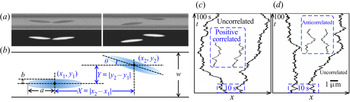
Coaxial  $({Y/w \in [0,0.1)} )$ and off-axis
 $({Y/w \in [0.5,0.7)} )$ ellipsoid pairs in the q1D channel. (a) Bright field (upper) and fluorescent (lower) microscopy images of the coaxial (left) and off-axis (right) ellipsoid pairs. (b) Schematic diagram of sample geometry and ellipsoid separation. (c,d) Axial trajectories x(t) (shifted 10 μm closer for clarity) of the coaxial (c) and off-axis (d) ellipsoid pairs; Insets are zoom-in views of the 10 s trajectories in the blue dashed boxes when X is less than the screening length XSC. Aspect ratio p = 7.5 and channel width w = 6 μm.

The remainder of the paper is organized as follows. We first describe the experimental system and the parameters of different samples in § 2. Experimental results of the T–T, R–R and T–R hydrodynamic couplings and comparison with other experiments are presented in § 3. The aim of § 4 is to provide a simple theoretical model for experimental results. Section 4.1 presents the dumbbell-in-cylinder model. Section 4.2 compares the experimental results with the model. The aim of § 5 is to make a comprehensive connection between experimental results and the model by the finite element numerical simulations. Section 5.1 compares with the simulation, experimental and theoretical results and § 5.2 demonstrates the flow field induced by a moving ellipsoid in a cylinder, which qualitatively explains the experimental results and the theoretical prediction. Finally, the work is summarized and concluded in § 6. Discussions and comparisons between the experimental, theoretical and numerical results can be found in §§ 5.1, 5.2 and 6.
2. Experimental systems
The sample cell comprised a polydimethysiloxane (PDMS) substrate with long straight microgrooves and a glass slide. The substrate and slide were separated by two 100 μm-thick spacers. First, we placed a droplet of aqueous suspension of colloidal ellipsoids onto the glass slide. The dilute colloidal suspension was absorbed into the sample cell due to the capillary force. Then, we quickly sealed the sample cell with epoxy glue. After approximately 30 min, the colloidal ellipsoids sediment onto the bottom of the microgrooves in the PDMS substrates. Finally, the Brownian motions of the colloidal ellipsoids in the grooves were observed under an optical microscope and recorded using a charge-coupled device camera at 10 frames per second (see figure 1a). The centre-of-mass (CM) positions (x, y) and orientations θ of individual ellipsoids (see figure 1b) were tracked according to our image processing algorithm with an angular resolution of 1° and spatial resolutions of 0.07 and 0.04 μm along the long and short axes, respectively (Zheng & Han Reference Zheng and Han2010).
To make the microgrooves, we fabricated lines of photoresist with widths of w = 4, 5 and 6 μm; a height of d = 5 μm; and a length of l = 1 cm on a silicon wafer through photolithography. Subsequently, the line patterns of the photoresist mask were printed on the PDMS substrate using soft lithography to form upper-side-open microgrooves with rectangular cross-sections and the same w, d and l. The PDMS rectangular grooves have sharp corner edge and <100 nm surface roughness on the upper surface and bottom.
In bright-field microscopy, the position of an ellipsoid cannot be very accurately measured due to the interference from the nearby channel edges. To accurately track the ellipsoids, we fabricated ellipsoids by stretching fluorescent spheres (Han et al. Reference Han, Alsayed, Nobili and Yodh2009; Zheng & Han Reference Zheng and Han2010) and imaged the ellipsoids under fluorescent microscopy (see figure 1a). Briefly, we added 3.26 μm-diameter fluorescent polystyrene (PS) spheres (0.5% by weight) into an aqueous solution of polyvinyl alcohol (PVA) (12% by weight) in a Petri dish, and heated and stretched the solid PVA film after water evaporation. The PS spheres embedded in the PVA film were stretched into ellipsoids at 110 °C, which is above the glass transition temperatures of PVA (Tg = 85 °C) and PS (Tg = 90 °C). After cooling to room temperature, the PVA was dissolved and washed away with deionized water several times. We fabricated five batches of ellipsoids with aspect ratios  $p = a/b = 1.8$, 2.2, 2.8, 5.2 and 7.5, where a and b were the semimajor and semiminor axes, respectively. The polydispersity of p was carefully controlled to less than 3%. The size ratios between the ellipsoids and the channel widths were chosen to enable quantitative exploration of the effects of particle anisotropies and degree of channel confinement on HIs, and to limit the particles’ orientational degrees of freedom to a small range by the narrow channel confinement. Next, 7 mM sodium dodecyl sulphate was added to stabilize the suspension (Zheng & Han Reference Zheng and Han2010). The pair potential between two ellipsoids was calculated from
 $U(X) ={-} {k_B}T\,\textrm{ln}\,g(X)$ according to the Boltzmann distribution at a low density where the multibody effect is negligible. Here, X is the CM separation along the axial direction (see figure 1b); and the one-dimensional radial distribution function,
 $g(X) = \langle \sum\nolimits_{i {\ne} 0} {\delta (x - {x_i})} \rangle /\rho$, was directly measured from the histogram of X normalized by the linear density
 $\rho = N/l$, where N is the total number of particles in the channel length l. The colloidal ellipsoids showed a hard-core pair potential, indicating that they can be regarded as hard particles without attractions or repulsions. According to the Boltzmann distribution, ellipsoids exhibit an exponential distribution along the z direction with a characteristic length of the gravitational height
 $h = {k_B}T/(mg) = 0.424\;{\rm \mu}\mathrm{m}$, where mg is the buoyancy weight of the ellipsoid. Here, h is much smaller than the particle size, indicating that the ellipsoids are heavy enough to sediment to the bottom of the channel with little fluctuations in the z direction. Such small distance between the particle and the bottom surface dominates particles’ drags, but does not qualitatively change HIs. It confines the angle fluctuation to merely 2°–5° for ellipsoids with aspect ratios ranging from 7.5 to 1.8. This is confirmed by the observation that ellipsoids’ centres and tips barely fluctuate out of the focal plane, i.e. the fluctuation is less than the 0.4 μm focal depth of the microscope objective.
The HIs were measured as functions of the particle CM separation (X, Y) (see figure 1b) with sufficient statistics for accurate measurements in different parameter regimes  $(p,w,Y/w)$ via very long (>24 h) observations for each sample with a certain p and w. The linear packing fraction
 $\phi = 2aN/l$ was moderately low
 $(0.05 \le \phi \le 0.3)$ to form many isolated ellipsoid pairs in channels; that is, other ellipsoids were more than 10a away and had little effect due to the short-range nature of HIs in the narrow grooves. In a long video of an equilibrium q1D dilute gas, all the video sections with isolated ellipsoid pairs (i.e. X < 10a and other particles >10a away) are used for HI measurements. Both approaching and receding motions of two ellipsoids are observed.
3. Experimental results
3.1. The x–x, x–θ, θ–θ, coupling diffusivities
The HIs of ellipsoid pairs are characterized by the x–x, θ–θ and x–θ coupling diffusivities, as follows:
 \begin{equation}\left\{\begin{array}{@{}c} {D_C^{xx} = \langle \Delta
{x_1}\Delta {x_2}\rangle /(2t),}\\ {D_C^{\theta \theta } =
\langle \Delta {\theta_1}\Delta {\theta_2}\rangle /(2t),}\\
{D_C^{x\theta } = \langle \Delta {x_1}|{\Delta {\theta_2}}
|\rangle /(2t) ={-} \langle |{\Delta {\theta_1}} |\Delta
{x_2}\rangle /(2t) ={-} D_C^{\theta x},} \end{array}\right.\end{equation}
where  $\Delta {x_i}$ is the CM displacement along the channel axis, and
 $\Delta {\theta _i}$ is the angular displacement with
 $- {\rm \pi} /2 \le \theta \le {\rm \pi} /2$ of ellipsoid i during time interval t (see figure 1b). Here
 $\langle \;\rangle$ is an average over trajectories of all isolated pairs at all times from experimental trials. The first equation in (3.1) has been used in previous studies about colloidal spheres (Cui et al. Reference Cui, Diamant and Lin2002, Reference Cui, Diamant, Lin and Rice2004; Mazo Reference Mazo2002; Valley et al. Reference Valley, Rice, Cui, Ho, Diamant and Lin2007; Diamant Reference Diamant2009; Novikov et al. Reference Novikov, Rice, Cui, Diamant and Lin2010), but the latter two about rotational motions have not been applied to colloidal experiments. In the diffusion matrix (Montgomery & Berne Reference Montgomery and Berne1977; Mazo Reference Mazo2002)
 $\boldsymbol{D}(X,Y)$ (see (1.1)),
 $D_C^{xx}$,
 $D_C^{\theta \theta }$ and
 $D_C^{x\theta }$ are the off-diagonal terms of the diffusion tensors
 ${\boldsymbol{D}^{\boldsymbol{xx}}}$,
 ${\boldsymbol{D}^{\boldsymbol{x\theta }}}$, and
 ${\boldsymbol{D}^{\boldsymbol{\theta \theta }}}$, while the diagonal terms are the self-diffusivities
 $D_S^{xx} \equiv \langle \Delta x_1^2\rangle /(2t)$,
 $D_S^{\theta \theta } \equiv \langle \Delta \theta _1^2\rangle /(2t)$ and
 $D_S^{x\theta } \equiv \langle \Delta {x_1}\Delta {\theta _1}\rangle /(2t)$.
The experimental results of  $D_C^{xx}(X)$,
 $D_C^{\theta \theta }(X)$ and
 $D_C^{x\theta }(X)$ at different degrees of off-axial distance
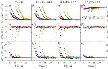
 $Y/w$ are shown in figure 2 for different p and in figure 3 for different w. The effects of
 $(w,Y/w)$ have not been explored even for T–T HIs of two spheres. In our experiment, they all show strong couplings at small X which decay with increasing X and vanish beyond XSC, reflecting a screening effect of the channel confinement on the HIs. The screening length
 ${X_{SC}}$ is defined as the minimal X where
 $|{{D_C}(X)} |\le 0.1{|{{D_C}(X)} |_{MAX}}$. The screening of HIs results in uncorrelated axial trajectories of ellipsoid pairs at
 $X > {X_{SC}}$ (see figure 1c,d). Interestingly, we find that
 $D_C^{xx}$ changes sign as
 $Y/w$ increases:
 $D_C^{xx} > 0$ at
 $Y/w < 0.5$ and X < XSC for various p (see figure 2a–c) and various w (see figure 3a–c), whereas
 $D_C^{xx} < 0$ at
 $Y/w > 0.5$ (see figures 2d and 3d). Such positive and negative x–x couplings are directly observed from the concerted single-file movements of ellipsoid pairs that are in the same directions at
 $Y/w < 0.1$ (see inset of figure 1c) but in opposite directions at
 $Y/w > 0.5$ (see inset of figure 1d). We emphasize that the positive axial HI
 $(D_C^{xx} > 0)$ dominates in q1D confinements with
 $w/b < 4$ which is too strong to allow particles passing each other, while the anomalous negative axial HI
 $(D_C^{xx} < 0)$ occurs in weak channel confinement
 $(w/b > 4)$. By contrast, for spherical particles in q1D or wide channels, only positive x–x couplings were observed (Cui et al. Reference Cui, Diamant and Lin2002; Lin et al. Reference Lin, Cui, Lee and Yu2002; Novikov et al. Reference Novikov, Rice, Cui, Diamant and Lin2010; Misiunas et al. Reference Misiunas, Pagliara, Lauga, Lister and Keyser2015). It is well known that the single-file movements of the spheres occurred only in q1D confinements (Cui et al. Reference Cui, Diamant and Lin2002; Lin et al. Reference Lin, Cui, Lee and Yu2002; Misiunas et al. Reference Misiunas, Pagliara, Lauga, Lister and Keyser2015). By contrast, our result shows that single-file diffusions of ellipsoids can occur in wide channels because two off-axis ellipsoids tend to separate apart
 $(D_C^{xx} < 0)$ when they get close to each other.
The experimental coupling diffusivities of ellipsoid pairs with different aspect ratio p as functions of interparticle distance  $(X,Y)$ in a channel of width w = 6 μm. Here (a–d)
 $D_C^{xx}$, (e–h)
 $D_C^{\theta \theta }$ and (i–l)
 $D_C^{x\theta }$. The transverse interparticle separation
 $Y/w \in [0,0.1)$,
 $[0.1,0.3)$,
 $[0.3,0.5)$ and
 $[0.5,0.7)$ in (a,e,i), (b,f,j), (c,g,k) and (d,h,l), respectively.

The experimental results of coupling diffusivities of ellipsoid pairs of aspect ratio p = 5.2 as functions of interparticle separation (X, Y) in channels of different width w. Here (a–d)  $D_C^{xx}$, (e–h)
 $D_C^{\theta \theta }$ and (i–l)
 $D_C^{x\theta }$. The transverse interparticle separation
 $Y/w \in [0,0.1)$,
 $[0.1,0.3)$,
 $[0.3,0.5)$ and
 $[0.5,0.7)$ in (a,e,i), (b,f,j), (c,g,k) and (d,h,l), respectively.

The θ–θ coupling is negative  $(D_C^{\theta \theta } < 0)$ at X < XSC for various p, w and
 $Y/w$ (see figures 2e–h and 3e–h), indicating that an ellipsoid's clockwise rotation tends to induce its neighbour's anticlockwise rotation. The x–θ coupling is positive
 $(D_C^{x\theta } > 0)$ (see figures 2i–l and 3i–l), indicating that an ellipsoid tends to rotate away from the channel axis as a neighbour approaches, and vice versa.
The screening lengths measured from figures 2 and 3 for various p and w are shown in figure 4. We find that XSC linearly increases with the long axis of ellipsoids (see figure 4a), leading to a rapid amplification of XSC with particles’ shape anisotropy. For the same p, XSC slowly increases with w (see figure 4b), reflecting a slightly stronger screening of HIs in a narrower channel. These results indicate that XSC is much more sensitive to the particle elongation than the channel width in upper-side-open groove channels. By contrast, XSC is on the length scale of w for colloidal spheres in the upper-side-open groove channels (Lin et al. Reference Lin, Cui, Lee and Yu2002; Valley et al. Reference Valley, Rice, Cui, Ho, Diamant and Lin2007). Therefore, particle elongation can extend the effective range of HIs exceeding the channel width  $({X_{SC}} \gg w)$ as shown in figure 4(b). In addition, we find that
 ${X_{SC}}/a$ is the largest for
 $D_C^{xx}$ and the smallest for
 $D_C^{\theta \theta }$, indicating a stronger suppression of rotational HIs than axial translational HIs by the channel confinement. Particles at different
 $Y/w$ have similar behaviours of XSC.
The screening lengths XSC (symbols) for  $D_C^{xx}$,
 $D_C^{\theta \theta }$ and
 $D_C^{x\theta }$ of the coaxial ellipsoid pairs
 $({Y/w \in [0,0.1)} )$. Here (a) XSC for different p and w = 6 μm and (b) XSC for different w and p = 7.5. The lines are linear fittings.

The HIs can also be characterized by the Pearson correlation coefficient (Misiunas et al. Reference Misiunas, Pagliara, Lauga, Lister and Keyser2015):  ${\rho ^{xx}} \equiv \textrm{cov(}\Delta {x_1},\Delta {x_2})/(\sigma (\Delta {x_1})\sigma (\Delta {x_2}))$ and similarly defined
 ${\rho ^{\theta \theta }}$ and
 ${\rho ^{x\theta }}$, where cov is the covariance,
 $\sigma $ is the standard deviation. They are equivalent to the normalized hydrodynamic coupling diffusivities
 ${\rho ^{xx}} = D_C^{xx}/D_S^{xx}$,
 ${\rho ^{\theta \theta }} = D_C^{\theta \theta }/D_S^{\theta \theta }$ and
 ${\rho ^{x\theta }} = D_C^{x\theta }/{(D_S^{xx}D_S^{\theta \theta })^{1/2}}$, which exclude the influence of channel confinement and particle anisotropy on self-diffusivities and enable a more precise comparison of HIs in different regimes of parameters
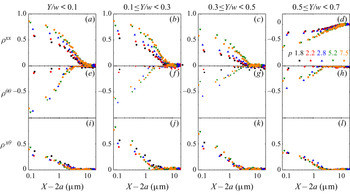
 $(p,w,Y/w)$ (Riley, Hobson & Bence Reference Riley, Hobson and Bence2006; Misiunas et al. Reference Misiunas, Pagliara, Lauga, Lister and Keyser2015). Figure 5 presents
 ${\rho ^{xx}}$,
 ${\rho ^{\theta \theta }}$ and
 ${\rho ^{x\theta }}$ as functions of the tip-to-tip distance of the ellipsoid pair. For the same tip-to-tip distance, the absolute value
 $|{{\rho^{xx}}} |$ increases more than one time as p increasing from 1.8 to 7.5 (see figure 5a–d), reflecting an enhanced T–T HIs for more anisotropic particles. Here
 $|{{\rho^{\theta \theta }}} |$ is non-monotonic with p and reaches the maximum at
 $p = 2.8$ (see figure 5e–h), reflecting the strongest R–R HIs at medium aspect ratios. We attribute the weak R–R HI as the small torque of the short moment arm for small p and the suppression from the channel confinement for large p. Here
 $|{{\rho^{xx}}} |$ and
 $|{{\rho^{\theta \theta }}} |$ decrease at larger
 $Y/w$, reflecting the suppression of T–T and R–R HIs for off-axis particle pairs which are closer to the channel walls. By contrast, figure 5(i–l) show that the maximum
 ${\rho ^{x\theta }}$ appears at middle
 $Y/w$, reflecting the strongest T–R HIs for moderate off-axis particles. The non-monotonic changes of
 ${\rho ^{\theta \theta }}$ with p (see figure 5e–h) and
 ${\rho ^{x\theta }}$ with
 $Y/w$ (see figure 5i–l) reflect non-trivial θ–θ and x–θ couplings. We explain these experimental results based on a theoretical model and low-Reynolds-number numerical simulation in the following sections.
The Pearson correlation coefficients of coupling diffusivities of ellipsoid pairs as functions of the interparticle tip-to-tip distance  $(X - 2a,Y)$ in a channel of width w = 6 μm. Here (a–d)
 ${\rho ^{xx}}$, (e–h)
 ${\rho ^{\theta \theta }}$ and (i–l)
 ${\rho ^{x\theta }}$. The transverse interparticle separations
 $Y/w \in [0,0.1)$,
 $[0.1,0.3)$,
 $[0.3,0.5)$ and
 $[0.5,0.7)$ in (a,e,i), (b,f,j), (c,g,k) and (d,h,l), respectively.

3.2. The y–y and y–θ coupling diffusivities
We next measure HIs about the transverse displacements by the y–y and y–θ coupling diffusivities as functions of (X, Y):  $D_C^{yy} = \langle \Delta {y_1}\Delta {y_2}\rangle /(2t)$ and
 $D_C^{y\theta } = \langle \Delta {y_1}\Delta {\theta _2}\rangle /(2t) = \langle \Delta {\theta _1}\Delta {y_2}\rangle /(2t) = D_C^{\theta y}$ in figure 6, where
 $\Delta {y_i}$ is the CM displacement of ellipsoid i in the transverse direction of the channel during time interval t. Here
 $D_C^{xx}(X)$ and
 $D_C^{yy}(X)$ of two spheres have been measured in three dimensions (Meiners & Quake Reference Meiners and Quake1999) and quasi-two dimensions (Cui et al. Reference Cui, Diamant, Lin and Rice2004; Valley et al. Reference Valley, Rice, Cui, Ho, Diamant and Lin2007; Diamant Reference Diamant2009). In the present study, we comprehensively measure
 $D_C^{xx}$,
 $D_C^{\theta \theta }$
 $D_C^{x\theta }$,
 $D_C^{yy}$ and
 $D_C^{y\theta }$ for ellipsoid pairs as a function of X and Y (see figures 2, 3 and 6).
The experimental results of y–y and y–θ coupling diffusivities. Here (a,b)  $D_C^{yy}$ and (c,d)
 $D_C^{y\theta }$ indicate no hydrodynamic coupling. Ellipsoid pairs with different p and at different axial interparticle distance X in a channel of w = 6 μm. (a,c) Coaxial
 $(Y/w \in [0,0.1))$ and (b,d) off-axis
 $(Y/w \in [0.5,0.7))$ ellipsoid pairs.

Figure 6 shows that  $D_C^{yy}(X)$ and
 $D_C^{y\theta }(X)$ are nearly zero for different p and
 $Y/w$, reflecting vanishing y–y and y–θ couplings. This is attributed to the strong suppression of transverse motion in channel confinement as shown from the very small fluctuations in the transverse trajectories of ellipsoids (see figure 7a). In addition, we observe that two neighbouring ellipsoids with 2a < X < XSC tend to locate symmetrically in the transverse direction about the central axis (y = 0) of the channel, that is,
 ${y_1}(t)\; = \; - {y_2}(t)$ (see figures 1a,b and 7); and the isolated single ellipsoids tend to equilibrate on the central axis, that is,
 $\; |{y(t)} |\; < \; 0.05w$ (see figure 7a). Note that X > 2a always hold since the ellipsoids cannot pass by each other in the narrow channel. Similar phenomena were observed in constant microfluidic flows in which the isolated polymers diffused towards the channel central axis (Usta, Ladd & Butler Reference Usta, Ladd and Butler2005) and the adjacent spherical droplets located symmetrically about the central axis and form zigzag patterns (Beatus, Tlusty, & Bar-Ziv Reference Beatus, Tlusty and Bar-Ziv2006; Fleury et al. Reference Fleury, Schiller, Thutupalli, Gompper and Seemann2014). These phenomena have been interpreted as resulting from the dipolar flow field around each particle in the channel confinement (Uspal & Doyle Reference Uspal and Doyle2014). However, the HIs and diffusion behaviours of particles due to the dipolar flow have not been measured. Our results indicate that the channel confinement suppresses the transverse motion much more than the rotational motion due to the large viscous drag along the ellipsoid short-axis. That is to say, the effect of the transverse component of a local dipolar flow created by a moving particle imposes a torque on the other particle and induces a rotational motion of that particle rather than a transverse motion.
(a) Typical transverse positions  $y(t)/w$ of an ellipsoid pair with 2a < X < XSC (blue curves) and a single ellipsoid (black curve). The channel boundary is at
 $Y/w$ = ±0.5. (b) The corresponding histogram of the transverse positions
 $H({y_1}/w)$ and
 $H({y_2}/w)$ of the ellipsoid pair with 2a < X < XSC (symbols) and the Gaussian fits (curves). The aspect ratio p = 7.5, and the channel width w = 6 μm.

4. Theoretical analysis
4.1. Dumbbell-in-cylinder model
The flow field created by a moving particle is usually estimated using the point force (Stokeslet) approximation (Batchelor Reference Batchelor1970; Cui et al. Reference Cui, Diamant and Lin2002, Reference Cui, Diamant, Lin and Rice2004; Hernández-Ortiz, de Pablo & Graham Reference Hernández-Ortiz, de Pablo and Graham2006; Valley et al. Reference Valley, Rice, Cui, Ho, Diamant and Lin2007; Diamant Reference Diamant2009; Novikov et al. Reference Novikov, Rice, Cui, Diamant and Lin2010). For example, a spherical particle, an elongated particle and a long-thin rod or fibre are often modelled as a point force (Cui et al. Reference Cui, Diamant and Lin2002, Reference Cui, Diamant, Lin and Rice2004; Valley et al. Reference Valley, Rice, Cui, Ho, Diamant and Lin2007; Diamant Reference Diamant2009; Novikov et al. Reference Novikov, Rice, Cui, Diamant and Lin2010), a dumbbell of two point forces (Hernández-Ortiz et al. Reference Hernández-Ortiz, de Pablo and Graham2006; Bukowicki, Gruca, & Ekiel-Jeżewska Reference Bukowicki, Gruca and Ekiel-Jeżewska2014) and a line of point forces (Batchelor Reference Batchelor1970; Di Leonardo et al. Reference Di Leonardo, Cammarota, Bolognesi, Schäfer and Steinhart2011; de Graaf et al. Reference de Graaf, Menke, Mathijssen, Fabritius, Holm and Shendruk2016), respectively. The T–T hydrodynamic coupling of colloidal spheres has been described by treating the moving sphere as a point force at the sphere centre (Cui et al. Reference Cui, Diamant and Lin2002, Reference Cui, Diamant, Lin and Rice2004; Valley et al. Reference Valley, Rice, Cui, Ho, Diamant and Lin2007; Diamant Reference Diamant2009; Novikov et al. Reference Novikov, Rice, Cui, Diamant and Lin2010). The translation of a spheroid in unbounded flow has been described by a line distribution of Stokeslets between the foci (Chwang & Wu Reference Chwang and Wu1976). Here, we proposed a simplified dumbbell-in-cylinder model to estimate the T–T, R–R and T–R coupling of two ellipsoids in channels. This model is based on the following three approximations as illustrated in figure 8 and summarized in table 1. (i) The motion of an ellipsoid is treated as a dumbbell of point forces  $(\boldsymbol{F},\boldsymbol{F^{\prime}})$, that is to say, the effect of the flow field induced by an ellipsoid on the other is equivalent to exerting
 $(\boldsymbol{F},\boldsymbol{F^{\prime}})$ on the fluid. The dumbbell length is 2XOF along the long axis with the centre coinciding with the ellipsoid's CM. (ii) The HIs between two ellipsoids are dominated by the point-force pair F1 and F2 near the centre of the two ellipsoids. Here
 ${\boldsymbol{F_1^{\prime}}}$ and
 ${\boldsymbol{F}_2^{\prime}}$ at the far ends can be neglected due to the strong screening of HIs in the channel. (iii) The confinement effect of a rectangular groove with an open side is equivalent to that of a cylinder with a radius R > w as confirmed in Cui et al. (Reference Cui, Diamant and Lin2002), Diamant (Reference Diamant2009) and Novikov et al. (Reference Novikov, Rice, Cui, Diamant and Lin2010). These assumptions hold well under the low Reynolds number (~10−6), the no-slip boundary conditions (Happel & Brenner Reference Happel and Brenner1983),
 $b \ll R$, and
 $(a - {X_{OF}}) \ll {X_F}$.
Schematic diagram of the dumbbell-in-cylinder model. (a) Rotational displacement  $\Delta \theta $ and (b) axial displacement
 $\Delta x$ of an ellipsoid pair between time = 0 (solid ellipses with filled circles) and time = t (dashed ellipses with open circles) in the effective cylinder (green dashed contours) of diameter 2R which is equivalent to a channel (solid blue lines) of width w. The subscript represents ellipsoid 1 or 2. The dumbbell of point forces
 $\boldsymbol{F}({x_F},{y_F})$ and
 $\boldsymbol{F^{\prime}}({x_{\mathrm{F^{\prime}}}},{y_{\mathrm{F^{\prime}}}})$ at the red circles are symmetric about the ellipsoid's CM (black circle) at (x, y) along the long axis. The transverse force
 ${F^y} ={-} {F^{\prime y}}$ in (a) and axial force
 ${F^x} = {F^{\prime x}}$ in (b) are proportional to the translational and axial displacements (red arrows)
 $\Delta {y_F} ={-} \Delta {y_{F^{\prime}}}$ and
 $\Delta {x_F} = \Delta {x_{F^{\prime}}}$, respectively (Goldfriend et al. Reference Goldfriend, Diamant and Witten2015).

Summary of the parameters, coordinates and coupling diffusivities in the experiment and theoretical models with subscript 1 or 2 denoting the left or right ellipsoid in figure 8.

According to this theoretical model, the T–T, T–R and R–R HIs between ellipsoids are treated as derived from the x–x, x–y and y–y components of the Stokeslet tensor. The axial translational and rotational displacements  $(\Delta x,\Delta \theta )$ of an ellipsoid can be represented by the axial and transverse displacements
 $(\Delta {x_F},\Delta {y_F})$ (see figure 8 and table 1). Consequently,
 ${D_C}(X,Y)$ of an ellipsoid pair in a channel can be approximately transformed into the dimensionless coupling diffusivities in an effective cylinder
 \begin{equation}\varDelta _F^{{\rm \mu} \nu } \equiv \langle \Delta {\boldsymbol{\mu} _{F1}}\Delta {\nu _{F2}}\rangle /(2t{k_B}T/6\boldsymbol{\pi} \eta R),\end{equation}
as functions of the rescaled axial and transverse separations  ${X_F}/R = (X - 2{X_{OF}})/R$ and
 ${Y_F}/R \approx Y/R$ (see figure 8 and table 1), where μ, ν = x or y and η is the fluid viscosity. By substituting the Stokes-flow Oseen tensor in a cylinder derived from Liron & Shahar Reference Liron and Shahar1978 and Blake Reference Blake1979 into (4.1), we obtained the theoretical equations
 \begin{align}
\varDelta _F^{{\rm \mu} \nu }({X_F}/R,{Y_F}/R) & = 6{\boldsymbol{\pi}
^2}\sum\limits_{k = 0}^3 \sum\limits_{n = 1}^3 \left\{
[a_{kn}^{{\rm \mu} \nu }({Y_F}/R)\,\textrm{cos}({\alpha _{kn}}
\cdot {X_F}/R)\right.\nonumber\\ & \quad \left.+\, b_{kn}^{{\rm \mu} \nu
}({Y_F}/R)\,\textrm{sin}({\alpha _{kn}} \cdot
{X_F}/R)]\,{\textrm{e}^{ - {\beta _{kn}} \cdot ({X_F}/R)}} \right.\nonumber\\ &
\left.\quad +\, c_{kn}^{{\rm \mu} \nu }({Y_F}/R)\,{\textrm{e}^{ -
{\gamma _{kn}} \cdot ({X_F}/R)}}\right\},\end{align}
where the values of  $({\alpha _{kn}},{\beta _{kn}},{\gamma _{kn}})$ and
 $(a_{kn}^{{\rm \mu} \nu },\; b_{kn}^{{\rm \mu} \nu },c_{kn}^{{\rm \mu} \nu })$ can be obtained from Liron & Shahar (Reference Liron and Shahar1978). Details about the theoretical expression are given in the Appendix (A). The theoretical results of
 $\varDelta _F^{{\rm \mu} \nu }$ at different
 $({X_F}/R,{Y_F}/R)$ in the dumbbell-in-cylinder model are shown in figure 9.
Theoretical estimates of the (a) x–x, (b) y–y and (c) x–y coupling diffusivities of point-force pairs as functions of the rescaled axial distance  ${X_F}/R$ and transverse distance
 ${Y_F}/R$ calculated from (4.2).

4.2. Comparisons between the experimental and theoretical results
We quantitatively compare the experimental  ${D_C}$ with the theoretical prediction of the aforementioned model in figure 10. The two parameters XOF and R in different
 $(p,w,Y/w)$ regimes can be fitted from two out of three couplings
 $\Delta _F^{xx},\;\Delta _F^{yy}$ and
 $\varDelta _F^{xy}$. For example, the fitted XOF and R from
 $\varDelta _F^{xx},\;\varDelta _F^{yy}$ can describe
 $\varDelta _F^{xy}$ well, and have no discernable difference from their best fits from all the three couplings, indicating that the dumbbell-in-cylinder model is effective. Moreover, figure 11(a) shows that R fitted at a certain
 $(w,Y/w)$ is robust at different p, indicating that R is a good parameter for describing the effects of the channel without the effects of ellipsoids. Figure 11(d) shows that XOF at a certain p is robust at different
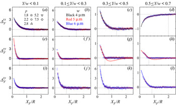
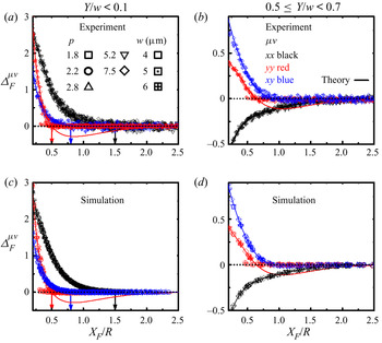
 $(w,Y/w)$, indicating that XOF is a good parameter for describing the effects of particles without the effects of the channel. We find that the theoretical model can describe the experimental data well by taking only the leading terms. As depicted in figure 10, the experimental
 ${\varDelta _F}({X_F}/R)$ (symbols) for all p and w at each
 $Y/w$ collapse onto the theoretical curves at the corresponding
 $Y/R$, suggesting a general mechanism of the Stokes-flow-induced hydrodynamic couplings. The experimental positive and negative x–x couplings of ellipsoid pairs at
 $Y/w < 0.5$ (see figures 2a–c and 3a–c) and
 $Y/w > 0.5$ (see figures 2d and 3d) are described well by the theoretical
 $\varDelta _F^{xx} > 0$ at
 ${Y_F}/R < 0.5$ (see figure 10a–c) and
 $\varDelta _F^{xx} < 0$ at
 ${Y_F}/R > 0.5$ (see figure 10d), respectively. The negative θ–θ (see figures 2e–h and 3e–h) and positive x–θ (see figures 2i–l and 3i–l) couplings of ellipsoid pairs agree with the theoretical
 $\varDelta _F^{yy} > 0$ (see figure 10e–h) and
 $\varDelta _F^{xy} > 0$ (see figure 10i–l). These consistent results reflect that the axial and transverse flows drive the axial and rotational motion of an ellipsoid, and T–T, R–R and T–R couplings reflect well the effect of HIs mediated by the x–x, y–y and x–y components of the induced flow. A reverse sign in
 $\varDelta _F^{yy}$ at
 ${X_F}/R\sim 1.0$ is predicted to arise from the alternating signed eddies of the Stokeslet along the channel (Liron & Shahar Reference Liron and Shahar1978; Blake Reference Blake1979), which is not observed experimentally here for ellipsoids nor for colloidal spheres previously (Novikov et al. Reference Novikov, Rice, Cui, Diamant and Lin2010). This discrepancy probably occurs because the surface of ellipsoid 1 between the point force and the tip, i.e. in the range of
 $({x_1} + {X_{OF}},{x_1} + a)$ near ellipsoid 2, produces positive
 $\varDelta _F^{yy}$ and vice versa, which superposes onto the negative
 $\varDelta _F^{yy}$ when the interparticle distance is more than the screening distance (
 $X > {X_{SC}}$ in the experiment, i.e.
 ${X_F} > X_{SC}^F$ in the model). An accurate description needs an integration over the whole surface of the particle, see the finite element numerical simulations in § 5 which fully recover the experimental
 $\varDelta _F^{yy}$; however, our dumbbell model approximates each ellipsoid only by one point force which can describe the average effect within the screening distance (
 ${X_F} < X_{SC}^F$ in figure 10), but deviates from the experimental
 $\varDelta _F^{yy}$ at
 ${X_F} > X_{SC}^F$. A more complicated model including multiple point forces may smear out the shallow negative
 $\varDelta _F^{yy}$ derived from our model with single Stokeslet approximation. Nevertheless, the agreement between the experimental and theoretical results in figure 10 ensures the validity and efficiency of this simple analytical model to describe the strongly screened HIs of ellipsoids in channel confinement.
Rescaled coupling diffusivities (a–d)  $\varDelta _F^{xx}$, (e–h)
 $\varDelta _F^{yy}$ and (i–l)
 $\varDelta _F^{xy}$ as functions of
 ${\xi ^x} = {X_F}/R$. The experimental data (symbols) for all p and w collapse onto the theoretical fittings of (4.2) (solid curves) except for the negative part of
 $\varDelta _F^{yy}$. The transverse separation of the ellipsoid pairs
 $Y/w \in [0,0.1)$, [0.1, 0.3), [0.3, 0.5) and [0.5, 0.7) in (a,e,i), (b,f,j), (c,g,k) and (d,h,l), respectively, with the fitted
 $Y/R = 0.04,\;0.14,\;0.32$ and 0.52. Vertical dashed lines mark the screening length
 $X_{SC}^F/R$.

The effective cylinder radius R and semidumbbell length XOF in the dumbbell-in-cylinder model. Here (a) R (symbols) versus  $Y/w$ obtained from figure 10 with linear fittings (solid lines) for experiments at different w and for all p; (b)
 $2R/w$ versus
 $Y/w$ rescaled from (a) with the linear fittings (solid lines); (c)
 $Y/R$ versus
 $Y/w$ rescaled from (a) with power-law fittings (solid curves), in (b,c), the black fitting curves are for square and triangle symbols; (d)
 ${X_{OF}}/a$ versus p for experiment (black squares) obtained from figure 10 and for numerical simulation (red circles) fitted from figure 13(c,d) with the curve guiding for the eyes.

Here,  $\varDelta _F^{xx},\;\varDelta _F^{yy}$ and
 $\varDelta _F^{xy}$ decay to zero at
 $X_{SC}^F/R \approx 1.5$, 0.5 and 0.8, respectively, for various p and w (vertical dashed lines in figure 10). Here
 $X_{SC}^F$ is the screening length of
 $\varDelta _F^{{\rm \mu} \nu }$. These different values of
 $X_{SC}^F/R$ indicate that the channel confinement suppresses the transverse local flow more than the axial flow. It explains the experimental phenomena in figure 4 that the screening length XSC is shortest for R–R coupling, intermediate for T–R coupling and longest for T–T coupling of two ellipsoids.
The fittings in figures 10 and 11 show that the cylinder radius R is sensitive to w and  $Y/w$ but not to p, while the dumbbell length XOF is sensitive to p but not to w and
 $Y/w$. The effects of channel confinement, i.e. w and
 $Y/w$ and particle anisotropy, i.e. p, on HIs are captured separately and quantitatively by the cylinder radius R and the dumbbell length XOF in our theoretical model. Figure 11(a) shows that R increases with w and linearly decreases as
 $Y/w$ increased. It reflects the stronger geometric confinement for particles closer to the channel wall can be linearly characterized by the smaller R. This results in that
 $R/w$ decreases and
 $Y/R$ increases with
 $Y/w$ (see figure 11b,c), respectively. Here
 $R/w$ or
 $Y/R$ show different trends as a function of
 $Y/w$ for channels with different cross-section shapes (figure 11b,c). Here, we discover that the fitted cylinder radius R is sensitive to both the degree of channel confinement
 $(w,Y/w)$ and the channel geometry
 $(w/d)$. As illustrated in figure 11(d),
 ${X_{OF}}/a$ increases with p and becomes asymptotic to 1 at large p, indicating that the effective point forces move toward the ellipsoid tips as the ellipsoid shape becomes more anisotropic. It predicts the increase of screening length
 ${X_{SC}} = X_{SC}^F + 2{X_{OF}}$ with a and p (see figure 4a). At small p, the logarithmic extrapolation of
 ${X_{OF}}/a$ in figure 11(d) correctly yields
 ${X_{OF}}/a = 0$ at p = 1 for spheres (Cui et al. Reference Cui, Diamant and Lin2002, Reference Cui, Diamant, Lin and Rice2004; Valley et al. Reference Valley, Rice, Cui, Ho, Diamant and Lin2007; Diamant Reference Diamant2009; Novikov et al. Reference Novikov, Rice, Cui, Diamant and Lin2010), reflecting the accuracy of the dumbbell model. As a result,
 ${X_{SC}} = X_{SC}^F$ for
 $D_C^{xx}$ of spheres in q1D groove channels (Cui et al. Reference Cui, Diamant and Lin2002) is much shorter than
 ${X_{SC}}$ for ellipsoids.
This model also explains the change in coupling strength at different parameter regimes in figures 2, 3 and 5. The more enhanced T–T coupling for ellipsoids of larger p (see figures 2a–d and 5a–d) arises from the larger  $\varDelta _F^{xx}$ for closer point-force pair, i.e. at shorter
 ${X_F} = X - 2{X_{OF}}$ due to longer
 ${X_{OF}}$ (see figure 11d). The weak θ–θ coupling for ellipsoids with
 $p \le 2.2$ (see figures 2e–h and 5e–h) can be attributed to that the moment arm
 ${X_{OF}}/a < 0.5$ is too small for slightly anisotropic particles to induce sufficient torque against thermal fluctuations. The θ–θ coupling decreases at
 $p \ge 5.2$ in figures 2e–h and 5e–h can be regarded as a result of the accumulation of negative
 $\varDelta _F^{yy}$ (see figures 9b and 10e–h) along the surface of largely anisotropic ellipsoids. The strongest T–R coupling at middle
 $Y/w$ (see figures 2i–l, 3i–l and 5i–l) is consistent with the maximum
 $\varDelta _F^{xy}$ at middle
 $Y/R$ (see figures 9c and 10i–l).
5. Numerical simulation
5.1. Comparisons between the simulation, experimental and theoretical results
We further perform three-dimensional finite element numerical simulations to verify the theoretical model by comparing the experimental, simulation and theoretical results, and to interpret the experimental HIs by calculating the flow field. The finite element numerical simulations are carried out using the software Comsol Multiphysics v5.2. To connect between the experimental system and theoretical model in the simulation, we use the geometries of two ellipsoids in an effective cylinder in the theoretical model, and input the parameters of the size (a, b) and axial and angular velocities  $(u,\omega )$ of the ellipsoids, and the fitted radius R of the cylinder for the groove channels with width w in the experiment. The two ellipsoids are separated with (X, Y) and symmetrically located about the central axis of the cylinder. We set no-slip boundary conditions on the surface of the ellipsoids and cylinder, and open boundary conditions at the two ends of the cylinder.
In order to simplify the calculation, we apply an instantaneous axial velocity  $u = ({u_1} = \Delta {x_1}/\Delta t,{u_2} = 0)$ or an instantaneous angular velocity
 $\omega = ({\omega _1} = \Delta {\theta _1}/\Delta t,\; {\omega _2} = 0)$ separately on the ellipsoid pair at each (X, Y) in a cylindrical channel with radius R (see figure 8), i.e. let one ellipsoid move and the other be at rest. We set the typical velocities
 $({u_1} = 1\;{\rm \mu} \mathrm{m}\;{\textrm{s}^{ - 1}},{\omega _1} = 2^\circ \;{\textrm{s}^{ - 1}})$ and
 $\Delta t = 0.1\;\textrm{s}$ according to the ellipsoid motions and frame rate in the experiment. We solve the Stokes equation in the cylinder and yield F and L from integrating the force distribution density over the ellipsoid surface. Thus each component term of
 $\boldsymbol{\zeta }$ is directly calculated through (1.3), and the matrix of diffusion tensors
 $\boldsymbol{D}$ at each (X, Y) is obtained through (1.2) (Montgomery & Berne Reference Montgomery and Berne1977; Mazo Reference Mazo2002). Due to the velocity-independency of
 $\boldsymbol{\zeta }$, a different set of velocity and
 $\Delta t$ will not change the results as long as (i) the Reynolds number is approximately 10−6 for micron-sized particles and (ii)
 ${x_1}(0) - 0.1a < {x_1}(\Delta t) < {x_1}(0) + 0.1a$ for ellipsoid 1. Here
 $0.1a$ is the bin size in the analysis of experimental results. Such a numerical method in the Comsol software has been used in the study of HIs of two spheres in a cylindrical channel in Misiunas et al. (Reference Misiunas, Pagliara, Lauga, Lister and Keyser2015). More benchmarking studies for the numerical method can be found in Dettmer et al. (Reference Dettmer, Pagliara, Misiunas and Keyser2014), Misiunas et al. (Reference Misiunas, Pagliara, Lauga, Lister and Keyser2015) and Misiunas & Keyser (Reference Misiunas and Keyser2019). The numerical simulation results of hydrodynamic coupling diffusivities
 $D_C^{xx}(X)$,
 $D_C^{x\theta }(X)$ and
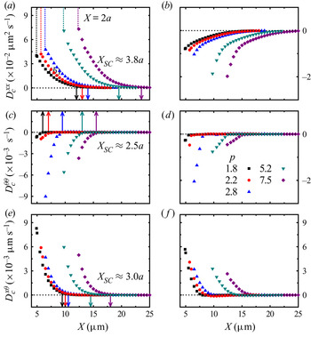
 $D_C^{\theta \theta }(X)$ for an ellipsoid pair in the effective cylinder are shown in figure 12, which reproduce the experimental results for the coaxial and most off-axis ellipsoid pairs in the groove channels in figure 2. The screening lengths
 ${X_{SC}}$ in the effective cylinder obtained in simulation (see figure 13) are consistent with those in the groove channels measured in experiments (see figure 5). Applying velocities in opposite directions gives the same quantitative results. The agreement between the experimental and simulation results confirm the validity of using the tube model to mimic the groove-like channel for the in-plane motions.
Numerical simulation results of coupling diffusivities  ${D_C}(X)$. (a,c,e) The coaxial (cylindrical radius R = 9.8 μm corresponding to
 $Y/w \in [0,0.1)$ and w = 6 μm in experiments) and (b,d,f) the off-axis (R = 6.5 μm,
 $Y/w \in [0.5,0.7)$ and w = 6 μm) ellipsoid pairs with different p. The vertical arrows mark the screening length XSC. Here
 ${D_C}$ is calculated from the simulation result of
 $\boldsymbol{\zeta }$ based on (1.2) in order to compare with the experimental
 ${D_\textrm{C}}$ in figure 2.

We further transform the numerical simulation results of  ${D_C}$ into
 $\varDelta _F^{{\rm \mu} \nu }$ and quantitatively compare them with the theoretical prediction by fitting the dumbbell length 2XOF. Figure 14 shows that both the simulation and experimental results of
 $\varDelta _F^{xx},\;\varDelta _F^{yy}$ and
 $\varDelta _F^{xy}$ coincide with their theoretical curves. The fitted XOF at each p from the simulation are the same in the three curves and consistent with those fitted from the experiment with only a 3%–5% systematic exceedance (see figure 11d). This exceedance probably reflects the larger hydrodynamic diameter than the geometrical diameter, which results in their effective aspect ratios slightly smaller than those used in the simulation.
The numerical simulation counterpart of figure 4. The screening lengths XSC (symbols) for  $D_C^{xx}$,
 $D_C^{\theta \theta }$ and
 $D_C^{x\theta }$ of the coaxial ellipsoid pairs at
 $Y/w \in [0,0.1)$. Here (a) XSC for different p and w = 6 μm and (b) XSC for different w and p = 7.5. The lines are linear fittings.

Rescaled coupling diffusivities  $\varDelta _F^{{\rm \mu} \nu }({X_F}/R)$. The experimental data (symbols in a,b) and the numerical simulation data (symbols in c,d) for all p and w collapse onto the theoretical curves (solid curves) of (4.2) with parameters R and XOF except for the negative part of
 $\varDelta _F^{yy}$. (a,c) The coaxial
 $({Y/w \in [0,0.1)} )$ and (b,d) the off-axis
 $({Y/w \in [0.5,0.7)} )$ ellipsoid pairs. The vertical arrows mark
 $X_{SC}^F/R$.

5.2. Flow field induced by a moving ellipsoid in a cylinder
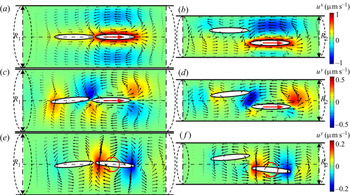
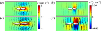
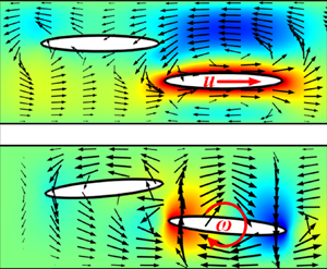
We measure the flow field induced by the moving ellipsoid in the numerical simulation to illustrate the effects of channel confinement and particle anisotropy on x–x, θ–θ and x–θ HIs. These flow fields in figures 15–17 are more complicated than those of colloidal spheres in strong q1D confinements (Cui et al. Reference Cui, Diamant and Lin2002; Misiunas et al. Reference Misiunas, Pagliara, Lauga, Lister and Keyser2015) where the coaxial flow induced by an axially moving sphere dominated, and only a positive x–x coupling was observed. Here, we can see that the axial and rotational motion of an ellipsoid actually reflects the axial and transverse component of the local flow field. For the coaxial ellipsoid pair in figure 15(a,c,e), a rightward axial motion of the right ellipsoid induces a rightward axial flow pulling the left ellipsoid (see figure 15a), which leads to the positive x–x coupling. The axial flow turns transversely near the ellipsoid tips causing the rotation of the left ellipsoid towards the axis (see figure 15c), which leads to the positive x–θ coupling. A rotation of an ellipsoid induces a whirling flow imposing a torque on the other ellipsoid in an opposite direction (see figure 15e), which leads to the negative θ–θ coupling.
Numerical simulation results of the flow fields created by the motion of an ellipsoid. (a–d) Translational and (e,f) rotational motions of the right ellipsoid. (a,c,e) The coaxial (cylinder radius R 1 = 9.8 μm corresponding to  $Y/w \in [0,0.1)$ and w = 6 μm in experiments) and (b,d,f) the off-axis (R 2 = 6.5 μm,
 $Y/w \in [0.5,0.7)$ and w = 6 μm) ellipsoid pairs with p = 7.5. The length and direction of the black arrows describe the local flow velocities. The colour represents the local flow speed
 ${u^\nu }$ in the ν direction.

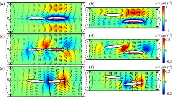
Simulation results of the flow fields created by the motion of an ellipsoid in the opposite direction to that in figure 15. (a–d) Translational and (e,f) rotational motions of the right ellipsoid. (a,c,e) The coaxial (R 1 = 9.8 μm corresponding to  $Y/w \in [0,0.1)$ and w = 6 μm in experiments) and (b,d,f) the off-axis (R 2 = 6.5 μm,
 $Y/w \in [0.5,0.7)$ and w = 6 μm) ellipsoid pairs with p = 7.5. The length and direction of the black arrows describe the local flow velocities. The colour represents the local flow speed
 ${u^\nu }$ in the ν direction.

Numerical simulation results of the flow fields created by the motion of an ellipsoid. (a,b) Translational and (c,d) rotational motions of the right ellipsoid. The cylinder of R = 9.8 μm corresponding to the coaxial  $({Y/w \in \; [0,0.1)} )$ ellipsoid pairs with (a,b) p = 2.2 and (c,d) p = 7.5 in a channel with w = 6 μm. The length and direction of the black arrows describe the local flow velocities. The colour represents the local flow speed
 ${u^\nu }$ in the ν direction.

By contrast, for the off-axis ellipsoid pair (see figure 15b,d,f), a rightward axial motion of the right ellipsoid induces a leftward backflow near the opposite sidewall repelling the left ellipsoid (see figure 14b), which leads to an anomalous negative x–x coupling as shown in the experiments, see figures 2(d) and 3(d). The weak channel confinement at  $w/b > 4$ enables the propagation of the backflow which is necessary for the negative x–x coupling. This repulsive HI ensures the single-file motion of ellipsoids in opposite directions even in channels moderately wider than 4b. It is in contrast to the strong q1D confinement where the piston-like motion of a sphere can only push other particles move in the same directions (Cui et al. Reference Cui, Diamant and Lin2002; Misiunas et al. Reference Misiunas, Pagliara, Lauga, Lister and Keyser2015). The turning flow between the two ellipsoids’ tips in figure 15(d) is much stronger than that for the coaxial ellipsoids in figure 15(c), which results in the most enhanced x–θ coupling at middle
 $Y/w$ in figures 2(i–l), 3(i–l) and 5(i–l). The whirling flow in figure 15(f) leads to similar negative θ–θ coupling as that of coaxial ellipsoids in figure 15(e). The smaller radius of the effective cylinder for more off-axis ellipsoids corresponds to stronger screening effect of the channel. As a result, the fast decay of flow field near the cylinder wall predicts weaker couplings for more off-axis ellipsoids as shown in figures 2, 3 and 5. Figure 16 shows that an ellipsoid moving in directions opposite to that in figure 15 produces similar patterns of the induced flow fields with reverse signs, which leads to the same behaviour of hydrodynamic couplings.
We further compare the flow fields of ellipsoids with different aspect ratios. Figure 17 shows that a more anisotropic ellipsoid induces a stronger flow in a larger range, which explains the longer XSC and stronger HIs for larger p (see figures 2–5). Especially, the weaker backflow at smaller p in figure 17(a,c) indicates that the backflow can be hardly probed by spheres, which may explain why the negative x–x coupling has not been observed before. The dipolar pattern of the local flow field in figures 14–16 confirms the validity of the dumbbell model for the ellipsoids. The transverse flow shows opposite directions at the two ends of an ellipsoid (see figure 15c–f). It verifies our interpretation for the suppressed transverse motion of the ellipsoids that the local flow induces mainly an effective torque rather than a transverse force. We find that the transverse flow in figure 15(e,f) decays much faster than the axial flow in figure 15(a,b), corresponding to the strongest screening of θ–θ coupling with shortest XSC and the weakest screening of x–x coupling with longest XSC by the channel confinement (see figures 2–5). Therefore, the effective region of the transverse flow is relatively shorter for longer ellipsoids. This screening effect on the anisotropic particles is featured by the longer XOF for larger p in the dumbbell model (see figure 11d). It results in the effective point force very close to the ellipsoid tip at  $p \ge 5.2$, which leads to a slight decrease in θ–θ coupling at
 $p \ge 5.2$ (see figures 2e–h and 5e–h).
The cylindrical tube with an appropriate diameter in our model reflects the average effects from all three walls and the open top of the groove. Particles have similar distances to the cylinder walls in the model, but a much closer distance to the bottom wall in the experiment. Such asymmetry with the lubrication flow in the bottom gap leads to a flow field distribution in the z direction different from that in the cylinder, which may make the flow field in the cylinder model quantitatively deviate from that in the experiment. Nevertheless, the HIs are still short-ranged due to the screening effect of the two sidewalls (figures 2 and 3) (Cui et al. Reference Cui, Diamant and Lin2002; Valley et al. Reference Valley, Rice, Cui, Ho, Diamant and Lin2007; Diamant Reference Diamant2009; Novikov et al. Reference Novikov, Rice, Cui, Diamant and Lin2010), thus whether the top of the groove is open or closed and whether the particles are closer to the bottom wall should not qualitatively change the results when the channel is not too narrow compared with the particle size. A qualitatively different case is a very narrow tube whose diameter is close to the particle size, where T–T HI is long-ranged due to the piston flow induced by the particle (Misiunas et al. Reference Misiunas, Pagliara, Lauga, Lister and Keyser2015). By contrast, for a cylinder with a radius much larger than the ellipsoid  $(R \gg b)$, the short-ranged swirl and back flows induced by an ellipsoid (figures 15–17) are similar to those induced by a Stokeslet (point force) in the cylinder model (Liron & Shahar Reference Liron and Shahar1978; Blake Reference Blake1979). The open-top channels and the cylinder with comparable scale
 $(1 < R/w\mathrm{\ \mathbin{\lower.3ex\hbox{$\buildrel< \over {\smash{\scriptstyle\sim}\vphantom{_x}}$}}\ }1.75)$ have similar confinement effects on HIs in the horizontal direction for ellipsoids much smaller than the channel width (
 $2.99 < w/b < 7.3$ in all cases) because
 $R/b$ and
 $w/b$ are of the same order. The lubrication flow in the narrow bottom gap does not affect the short-range nature of the HIs in the groove because the fluid can easily flow from the sidewalls or the open top. That is, the HIs are short-ranged and the similar swirl and back flows can be qualitatively expected for two ellipsoids either sediment to the bottom of an open-top channel or in the middle of a cylinder; the numerical results of two ellipsoids in a cylinder (figures 12 and 13) agree with the experimental results in the channel (figures 2 and 4); both experimental and numerical results are fitted by the model with consistent fitting parameters (figures 10, 11 and 14). Qualitatively, the decay length of flow field is comparable to w in the groove and comparable to R in the cylinder model, which is confirmed by the measured
 $0.8\mathrm{\ \mathbin{\lower.3ex\hbox{$\buildrel< \over {\smash{\scriptstyle\sim}\vphantom{_x}}$}}\ }X_{SC}^F/w\mathrm{\ \mathbin{\lower.3ex\hbox{$\buildrel< \over {\smash{\scriptstyle\sim}\vphantom{_x}}$}}\ }2$ and
 $0.5\mathrm{\ \mathbin{\lower.3ex\hbox{$\buildrel< \over {\smash{\scriptstyle\sim}\vphantom{_x}}$}}\ }X_{SC}^F/R\mathrm{\ \mathbin{\lower.3ex\hbox{$\buildrel< \over {\smash{\scriptstyle\sim}\vphantom{_x}}$}}\ }1.5$ for various p and w in figures 11 and 12. Therefore, the cylinder model with the Stokeslet approximation can capture the main features of the experimental T–T, T–R and R–R couplings (figures 10 and 11). Such a simple analytical cylinder model has successfully captured the main features of short-ranged T–T coupling between colloidal spheres in open-top grooves (Cui et al. Reference Cui, Diamant and Lin2002; Valley et al. Reference Valley, Rice, Cui, Ho, Diamant and Lin2007; Diamant Reference Diamant2009; Novikov et al. Reference Novikov, Rice, Cui, Diamant and Lin2010).
6. Conclusion
Our experiment, numerical simulation, and theory yield consistent results for non-trivial translational and rotational HIs in different parameter regimes of  $(p,w,Y/w)$ (figures 2–5, 10–14). All the parameters in the experiment and the model are summarized in table 1, including geometries, interparticle separations, displacements, coupling diffusivities, etc. The quantitative relations between the fitting parameters and
 $(p,w,Y/w)$ are shown in figure 11. The particle anisotropy amplifies the range of HIs. The negative R–R and positive T–R couplings non-monotonically change with p and
 $Y/w$, respectively. Particularly, the positive axial HI
 $(D_C^{xx} > 0)$ under strong q1D confinements
 $(w/b < 4)$ becomes anomalously negative
 $(D_C^{xx} < 0)$ under weak confinements
 $(w/b > 4)$ due to backflows in wider channels. This effect is stronger for ellipsoids with large p, which may explain its absence in previous observations of colloidal spheres. In conventional single-file diffusions, spheres are strongly confined in q1D channels and always exhibit positive axial HIs, which lead to the collective concerted motion of several neighbouring spheres (Pozrikidis Reference Pozrikidis1992; Wei et al. Reference Wei, Bechinger and Leiderer2000; Cui et al. Reference Cui, Diamant and Lin2002; Misiunas et al. Reference Misiunas, Pagliara, Lauga, Lister and Keyser2015). By contrast, the negative axial HIs of ellipsoids can effectively separate ellipsoids along a channel, leading to a single-file system in wide channels. Thus, single-file diffusion is not limited to strong q1D confinement, which is previously unexpected.
These distinct HIs and diffusion behaviours of particles in different parameter regimes could involve critical implications for the migration, morphology and self-organization of particles (Raven & Marmottant Reference Raven and Marmottant2009; Uspal, Eral & Doyle Reference Uspal, Eral and Doyle2013) in microfluids and the two-particle microrheology (Crocker et al. Reference Crocker, Valentine, Weeks, Gisler, Kaplan, Yodh and Weitz2000; Levine & Lubensky Reference Levine and Lubensky2000) in confined systems (Keen et al. Reference Keen, Yao, Leach, Di Leonardo, Saunter, Love, Cooper and Padgett2009). For example, the positive axial HI with  $D_C^{xx} > 0$ in q1D channel
 $(w/b < 4)$ could enhance the transport of multiple particles through channels (Misiunas et al. Reference Misiunas, Pagliara, Lauga, Lister and Keyser2015), whereas the negative axial HI with
 $D_C^{xx} < 0$ in weak confinement
 $(w/b > 4)$ could suppress the collective transport. Spherical particles in q1D channels exhibit interesting phonons and zigzag modes (Beatus et al. Reference Beatus, Tlusty and Bar-Ziv2006; Fleury et al. Reference Fleury, Schiller, Thutupalli, Gompper and Seemann2014; Uspal & Doyle Reference Uspal and Doyle2014). Our results suggest that these phenomena could be different and much richer for particles of different anisotropy in channels of different widths.
We find that the Stokeslet approximation is suitable not only for spherical particles (Cui et al. Reference Cui, Diamant and Lin2002) and slender bodies (Di Leonardo et al. Reference Di Leonardo, Cammarota, Bolognesi, Schäfer and Steinhart2011), but also for ellipsoids with different aspect ratios for which the configuration of Stokeslet objects depends on both the geometric confinement and the particle shape. This method can be applied to other anisotropic particles in channel confinement, which avoids the expensive computational cost with regard to the detailed surface geometries of particles and channels.
Acknowledgements
The authors thank G. Hu for the helpful discussion.
Funding
This work was supported by the National Natural Science Foundation of China (Z.Z.; grant number 11372314), (Y.W.; grant number U1738118 X.X.: grant number 11974038 and U1930402), the Strategic Priority Research Program of the Chinese Academy of Sciences (Y.W.; grant number XDB22040301); the Guangdong Basic and Applied Basic Research Foundation grant (Y.H.; grant number 2020B1515120067); and the Hong Kong Research Grants Council under the Collaborative Research Fund (Y.H.; grant number C6016–20G).
Declaration of interests
The authors report no conflict of interest.
Author contributions
Y.H. and Z.Z. conceived and designed the research. Z.Z carried out the experiment, simulation and data analysis, with the help from X.X, Y.H. and Y.W. The paper was written by Z.Z and Y.H. with the help from X.X. and Y.W. Supervision of and support for the work was carried out by Y.W. and Y.H. All authors discussed the results.
Appendix A. Theoretical expression of the dumbbell-in-cylinder model
We estimate the HI of two neighbouring ellipsoids in a channel by a dumbbell-in-cylinder model. The effect of flow field induced by the motion of an ellipsoid on the neighbouring ellipsoid is treated as equivalent to the flow field induced by the dumbbell of point forces (F, F′). For each ellipsoid, the positions of the two point forces are (xF, yF) and (xF ′, yF ′) on the long axis (see figure 1b and table 1), which are symmetric around the ellipsoid's CM at (x, y). Because  $\Delta \theta $ is small in the narrow channel,
 $\Delta {y_{F1}} = \Delta {\theta _1} \times {X_{OF}}$ for the left ellipsoid and
 $\Delta {y_{F2}} ={-} \Delta {\theta _2} \times {X_{OF}}$ for the right ellipsoid in figure 8, representing that the rotational motion of the ellipsoid is dominated by the transverse displacement of point (xF, yF). Hence, the axial translational motion
 $\Delta x = \Delta {x_F} = \Delta {x_{F^{\prime}}}$ and the rotational motion
 $\Delta {y_F} ={-} \Delta {y_{F^{\prime}}}$ are proportional to the axial force
 ${F^x} = {F^{\prime x}}$ and transverse force
 ${F^y} ={-} {F^{\prime y}}$, respectively. This dumbbell-in-cylinder model for ellipsoids in channel is a generalization of the point-force approximation for colloidal spheres in Cui et al. (Reference Cui, Diamant and Lin2002) and Novikov et al. (Reference Novikov, Rice, Cui, Diamant and Lin2010). The point-force approximation was used to describe the translational coupling of spheres, and our dumbbell-in-cylinder model enables representation of the translational, rotational and cross-couplings, as described subsequently. According to Appendix B of Liron & Shahar (Reference Liron and Shahar1978), the dimensionless hydrodynamic coupling tensor for a point force in a cylinder
 \begin{align}\varDelta _F^{{\rm \mu} \nu } \equiv D_{F,C}^{{\rm \mu} \nu }({X_F}/R,{Y_F}/R)/({k_B}T/6{\rm \pi} \eta R) = \langle \Delta {{\rm \mu} _{F1}}\Delta {\nu _{F2}}\rangle /(2t{k_B}T/6{\rm \pi} \eta R) = 6{\rm \pi} \eta R{G^{{\rm \mu} \nu }},\end{align}
with μ and ν denoting either x or y component. Here, the Stokes-flow Oseen tensor in the cylinder
 \begin{equation}{G^{{\rm \mu} \nu }} = {u^{{\rm \mu} \nu }}/(\eta R),\end{equation}
where η is the viscosity and R is the radius of the cylinder. By substituting (A2) into (A1), we obtain the dimensionless coupling diffusivity
 \begin{equation}\varDelta _F^{{\rm \mu} \nu } = 6{\rm \pi} {u^{{\rm \mu} \nu }}.\end{equation}
The dimensionless  ${u^{{\rm \mu} \nu }}({x_{F1}} = 0,{y_{F1}} = {y_1},{x_{F2}} = {X_F},{y_{F2}} = {y_2})$ is the fluid velocity at
 $({x_{F2}},{y_{F2}})$ in the μ direction induced by a unit point force at
 $({x_{F1}},{y_{F1}})$ pointing to the ν direction (Liron & Shahar Reference Liron and Shahar1978; Blake Reference Blake1979):
 \begin{equation}\left\{
\begin{aligned} \displaystyle{u^{xx}}({\xi^X},\; {\xi^{{y_1}}},\;
{\xi^{{y_2}}}) & =\sum\limits_{k ={-} \infty }^\infty
{\left\{ { - 2{\rm \pi} \sum\limits_{n = 1}^\infty
{{\textrm{e}^{ - {\beta_{kn}}{\xi^x}}}\,{\mathop{\rm
Im}\nolimits}
[{\textrm{e}^{\textrm{i}{\alpha_{kn}}{\xi^x}}}F_{1,kn}^{xx}({\xi^{{y_1}}},{\xi^{{y_2}}})]}
} \right.} \\& \quad\displaystyle\left. -\, {\rm \pi} \sum\limits_{n = 1}^\infty
{{\textrm{e}^{ - {\gamma_{kn}}{\xi^x}}}\,{\mathop{\rm
Im}\nolimits} [F_{2,kn}^{xx}({\xi^{{y_1}}},{\xi^{{y_2}}})]}
\right\},\\ \displaystyle{u^{\textrm{yy}}}({\xi^\textrm{X}},\;
{\xi^{{\textrm{y}_1}}},\; {\xi^{{\textrm{y}_2}}}) &
=\sum\limits_{k ={-} \infty }^\infty {\left\{ { -
2{\rm \pi} \sum\limits_{n = 1}^\infty {{\textrm{e}^{ -
{\beta_{kn}}{\xi^x}}}\,\textrm{Im}[{\textrm{e}^{\textrm{i}{\alpha_{kn}}{\xi^x}}}F_{1,kn}^{yy}({\xi^{{y_1}}},{\xi^{{y_2}}})]}
} \right.} \\ & \quad\displaystyle\left. - {\rm \pi}\sum\limits_{n =
1}^\infty {{\textrm{e}^{ -
{\gamma_{kn}}{\xi^x}}}\,\textrm{Im}[F_{2,kn}^{yy}({\xi^{{y_1}}},{\xi^{{y_2}}})]} \right\},\\
\displaystyle{u^{xy}}({\xi^X},\; \; {\xi^{{y_1}}},\;
{\xi^{{y_2}}}) & =\sum\limits_{k ={-} \infty }^\infty
{\left\{ {2{\rm \pi} \sum\limits_{n = 1}^\infty
{{\textrm{e}^{ -
{\beta_{kn}}{\xi^x}}}\,\textrm{Re}[{\textrm{e}^{\textrm{i}{\alpha_{kn}}{\xi^x}}}F_{1,kn}^{xy}({\xi^{{y_1}}},{\xi^{{y_2}}})]}
} \right.} \\& \quad\displaystyle\left. +\, {\rm \pi}\sum\limits_{n =
1}^\infty {{\textrm{e}^{ -
{\gamma_{kn}}{\xi^x}}}\,\textrm{Re}[F_{2,kn}^{xy}({\xi^{{y_1}}},{\xi^{{y_2}}})]}\right\}. \end{aligned}
\right.\end{equation}
Here,  ${\xi ^X} = |{{x_2} - {x_1}} |/R = {X_F}/R$,
 ${\xi ^{{y_1}}} = {y_1}/R$ and
 ${\xi ^{{y_2}}} = {y_2}/R$. Here Im and Re denote the imaginary and real parts of a complex number, respectively. Here also
 \begin{align}\left\{
\begin{aligned}
F_{j,kn}^{xx}({\xi^{{y_1}}},{\xi^{{y_2}}})\\ &
\quad=\dfrac{{{\psi^x}(s_{kn}^j,k,{\xi^{{y_1}}}){I_k}(s_{kn}^j{\xi^{{y_2}}})
+
[s_{kn}^j{\xi^{{y_2}}}{{I^{\prime}}_k}(s_{kn}^j{\xi^{{y_2}}})
+
{I_k}(s_{kn}^j{\xi^{{y_2}}})]{{\rm \pi} ^x}(s_{kn}^j,k,{\xi^{{y_1}}})}}{{{{D^{\prime}}_k}(s_{kn}^j)}},\\
& F_{j,kn}^{yy}({\xi^{{y_1}}},{\xi^{{y_2}}})\\ & \quad={{\left\{
{\dfrac{{{\psi^y}(s_{kn}^j,k,{\xi^{{y_1}}}){{I^{\prime}}_k}(s_{kn}^j{\xi^{{y_2}}})
+
{\varpi^y}(s_{kn}^j,k,{\xi^{{y_1}}})k{I_k}(s_{kn}^j{\xi^{{y_2}}})}}{{(s_{kn}^j{\xi^{{y_2}}})
+
{{\rm \pi} ^y}(s_{kn}^j,k,{\xi^{{y_1}}})s_{kn}^j{\xi^{{y_2}}}{{I^{\prime\prime}}_k}(s_{kn}^j{\xi^{{y_2}}})}}}
\right\}} / {{{D^{\prime}}_k}(s_{kn}^j)}},\\
& F_{j,kn}^{xy}({\xi^{{y_1}}},{\xi^{{y_2}}})\\ & \quad=-
\dfrac{{{\psi^y}(s_{kn}^j,k,{\xi^{{y_1}}}){I_k}(s_{kn}^j{\xi^{{y_2}}})
+
[s_{kn}^j{\xi^{{y_2}}}{{I^{\prime}}_k}(s_{kn}^j{\xi^{{y_2}}})
+
{I_k}(s_{kn}^j{\xi^{{y_2}}})]{{\rm \pi} ^y}(s_{kn}^j,k,{\xi^{{y_1}}})}}{{{{D^{\prime}}_k}(s_{kn}^j)}},
\end{aligned} \right.\end{align}
where Ik is the kth-order modified Bessel function of the first kind. Here  $s_{kn}^{j = 1} = {\alpha _{kn}} + \textrm{i}{\beta _{kn}}$ and
 $s_{kn}^{j = 2} = \textrm{i}{\gamma _{kn}}$ are two independent roots of
 ${D_k}(s) = s{I_k}(s)({I_{k - 1}}(s){I_{k + 1}}(s))^{\prime} - 2(s{I_k}(s))^{\prime}{I_{k - 1}}(s){I_{k + 1}}(s) = 0$. The detailed functions of
 $\psi (s,k,{\xi ^{{y_1}}})$,
 $\; \varpi (s,k,{\xi ^{{y_1}}})$ and
 ${\rm \pi} (s,k,{\xi ^{{y_1}}})$ are given in Liron & Shahar (Reference Liron and Shahar1978). By substituting (A5) into (A4), we obtain
 \begin{align}\left\{
\begin{aligned} {u^{xx}}({\xi^X},{\xi^{{y_1}}},\;
{\xi^{{y_2}}}) & = \sum\limits_{k ={-} \infty }^\infty
{\left\{ {2{\rm \pi} \sum\limits_{n = 1}^\infty
{[a_{kn}^{xx}({\xi^{{y_1}}},{\xi^{{y_2}}})\,\textrm{cos}({\alpha_{kn}}{\xi^X}) } } \right.} \\& \left. { \quad
+\, b_{kn}^{xx}({\xi^{{y_1}}},{\xi^{{y_2}}})\,\textrm{sin}({\alpha_{kn}}{\xi^X})]{\textrm{e}^{
- {\beta_{kn}}{\xi^X}}} +
{\rm \pi} \sum\limits_{n = 1}^\infty
{c_{kn}^{xx}({\xi^{{y_1}}},{\xi^{{y_2}}})\,{\textrm{e}^{ -
{\gamma_{kn}}{\xi^X}}}} } \right\}\!,\\
{u^{yy}}({\xi^X},{\xi^{{y_1}}},\; {\xi^{{y_2}}}) & =
\sum\limits_{k ={-} \infty }^\infty {\left\{ {2{\rm \pi} \sum\limits_{n = 1}^\infty
{[a_{kn}^{yy}({\xi^{{y_1}}},{\xi^{{y_2}}})\,\textrm{cos}({\alpha_{kn}}{\xi^X}) } } \right.} \\& \left. { \quad
+\,
b_{kn}^{yy}({\xi^{{y_1}}},{\xi^{{y_2}}})\,\textrm{sin}({\alpha_{kn}}{\xi^X})]\,{\textrm{e}^{
- {\beta_{kn}}{\xi^X}}} +
{\rm \pi} \sum\limits_{n = 1}^\infty
{c_{kn}^{yy}({\xi^{{y_1}}},{\xi^{{y_2}}})\,{\textrm{e}^{ -
{\gamma_{kn}}{\xi^X}}}} } \right\}\!,\\
{u^{xy}}({\xi^X},{\xi^{{y_1}}},\; {\xi^{{y_2}}}) & =
\sum\limits_{k ={-} \infty }^\infty {\left\{ {2{\rm \pi} \sum\limits_{n = 1}^\infty
{[a_{kn}^{xy}({\xi^{{y_1}}},{\xi^{{y_2}}})\,\textrm{cos}({\alpha_{kn}}{\xi^X})
} } \right.} \\ & \quad +
b_{kn}^{xy}({\xi^{{y_1}}},{\xi^{{y_2}}})\,\textrm{sin}({\alpha_{kn}}{\xi^X})]\,{\textrm{e}^{
- {\beta_{kn}}{\xi^X}}} + \left.
{{\rm \pi} \sum\limits_{n = 1}^\infty
{c_{kn}^{xy}({\xi^{{y_1}}},{\xi^{{y_2}}})\,{\textrm{e}^{ -
{\gamma_{kn}}{\xi^X}}}} } \right\}\!. \end{aligned}
\right.\end{align}
Here, the values of the parameters  ${\alpha _{kn}}$,
 ${\beta _{kn}}$ and
 ${\gamma _{kn}}$ are available in Liron & Shahar (Reference Liron and Shahar1978). Here
 $a_{kn}^{{\rm \mu} \nu }({\xi ^{{y_1}}},{\xi ^{{y_2}}}) ={-} {\mathop{\rm Im}\nolimits} [F_{1,kn}^{{\rm \mu} \nu }({\xi ^{{y_1}}},{\xi ^{{y_2}}})]$,
 $b_{kn}^{{\rm \mu} \nu }({\xi ^{{y_1}}},{\xi ^{{y_2}}}) ={-} Re [F_{1,kn}^{{\rm \mu} \nu }({\xi ^{{y_1}}},{\xi ^{{y_2}}})]$ and
 $c_{kn}^{{\rm \mu} \mathrm{\nu }}({\xi ^{{\textrm{y}_1}}},{\xi ^{{\textrm{y}_2}}}) ={-} \textrm{Im}[F_{2,kn}^{{\rm \mu} \nu }({\xi ^{{\textrm{y}_1}}},{\xi ^{{\textrm{y}_2}}})]$ for
 ${\rm \mu} = \nu $, and
 $a_{kn}^{{\rm \mu} \nu }({\xi ^{{y_1}}},{\xi ^{{y_2}}}) = Re [F_{1,kn}^{{\rm \mu} \nu }({\xi ^{{y_1}}},{\xi ^{{y_2}}})]$,
 $b_{kn}^{{\rm \mu} \nu }({\xi ^{{y_1}}},{\xi ^{{y_2}}}) = {\mathop{\rm Im}\nolimits} [F_{1,kn}^{{\rm \mu} \nu }({\xi ^{{y_1}}},{\xi ^{{y_2}}})]$ and
 $c_{kn}^{{\rm \mu} \nu }({\xi ^{{y_1}}},{\xi ^{{y_2}}}) = Re [F_{2,kn}^{{\rm \mu} \nu }({\xi ^{{y_1}}},{\xi ^{{y_2}}})]$ for
 ${\rm \mu} \ne \nu $.
In our experiments,  ${y_1} ={-} {y_2}$, as shown in § 3.2, that is,
 ${\xi ^{{y_1}}} ={-} {\xi ^{{y_2}}}$. By substituting (A6) into (A3) and taking
 $({\xi ^{{y_1}}} ={-} {\xi ^Y}/2,{\xi ^{{y_2}}} = {\xi ^Y}/2)$, we obtain (4.2) in § 4.1 of the main text. We find that the experimental data of
 $\varDelta _F^{{\rm \mu} \nu }({\xi ^X} = (X - 2{X_{OF}})/R,\; {\xi ^Y} = Y/R) = 6{\rm \pi} {u^{{\rm \mu} \nu }}({\xi ^X},{\xi ^Y})$ is well-described theoretically by taking k = 0, 1, 2, 3 and n = 1, 2, 3 in (A6) (see figures 9 and 10). Here XOF and R are obtained by fitting the three types of couplings:
 $\varDelta _F^{xx},\;\varDelta _F^{yy}$ and
 $\varDelta _F^{xy}$. Note that
 $\varDelta _F^{yy}$ mainly characterizes the θ–θ coupling, while
 $D_C^{yy}$ characterizes the y–y coupling.
To compare the simulation results of hydrodynamic couplings with the theoretical model, we fit the simulation results of the rescaled dimensionless coupling diffusivities (Liron & Shahar Reference Liron and Shahar1978; Cui et al. Reference Cui, Diamant and Lin2002)  $\varDelta _F^{{\rm \mu} \nu } \equiv D_{F,C}^{{\rm \mu} \nu }({X_F}/R = (X - 2{X_{OF}})/R,{Y_F}/R = Y/R)/({k_B}T/6{\rm \pi} \eta R)$ with the theoretical prediction and compare the fitting parameters in experiments and simulations. Here
 $\varDelta _F^{{\rm \mu} \nu }$ is calculated by transforming the hydrodynamic couplings
 ${\boldsymbol{D}_{\boldsymbol{C}}}$ of ellipsoids in (1.2) to
 $D_{F,C}^{{\rm \mu} \nu }$ of point forces through substituting the friction matrix (Reichert & Stark Reference Reichert and Stark2004)
 \begin{equation}{\boldsymbol{\zeta
}_{\boldsymbol{F}}} = \begin{pmatrix}
{{\boldsymbol{\zeta }^{xx}}}&{{\boldsymbol{\zeta }^{xy}}}\\
{{\boldsymbol{\zeta }^{yx}}}&{{\boldsymbol{\zeta }^{yy}}}
\end{pmatrix} = \begin{pmatrix}
{{\boldsymbol{\zeta }^{xx}}}&{{\boldsymbol{\zeta }^{x\theta
}}X_{OF}^{ - 1}}\\ {{\boldsymbol{\zeta }^{\theta
x}}{X_{OF}}^{ - 1}}&{{\boldsymbol{\zeta }^{\theta \theta
}}X_{OF}^{ - 2}} \end{pmatrix}\end{equation}
into  ${\boldsymbol{D}_{\boldsymbol{F}}} = {k_B}T\boldsymbol{\zeta }_{\boldsymbol{F}}^{ - 1}$ in the dumbbell-in-cylinder model. Thence, the dumbbell length
 $2{X_{OF}}$ is the only fitting parameter in the simulation, which agrees well to the experimental results in figure 11(d).