

Introduction
Since 1875, the region north of 60°N has warmed at a rate of 1.36°C per century, which is about twice as fast as the global average temperature (IPCC 2014). During the 1960s–2000s, temperature trends from Arctic Alaska indicated a pronounced warming over the region (Chapman and Walsh Reference Chapman and Walsh1993). During this period, an increase in shrub abundance was observed across the Arctic using repeat aerial photography (Myers-Smith and others Reference Myers–Smith, Forbes and Wilmking2011; Sturm and others Reference Sturm, Racine and Tape2001b). Observational and experimental studies also detected a recent increase in aboveground biomass, particularly for deciduous shrubs, linked to recent climate warming (Chapin and others Reference Chapin, Shaver and Giblin1995; Elmendorf and others Reference Elmendorf, Henry and Hollister2012; Hudson and Henry Reference Hudson and Henry2009; Huemmrich and others Reference Huemmrich, Gamon and Tweedie2010). The increasing trend of the Normalized Difference Vegetation Index (NDVI) in the Arctic, also known as ‘greening’, has been associated with a warming trend in the region (Jia and Howard Reference Jia and Howard2003; Myneni and others Reference Myneni, Keeling and Tucker1997; Stow and others Reference Stow, Hope and McGuire2004). Shrub rings indicate that warming is a primary contributor to shrub expansion in the Arctic (Forbes and others Reference Forbes, Fauria and Zetterberg2010; Tape and others Reference Tape, Hallinger and Welker2012). If the atmospheric heating in the region continues, a likely scenario could be the conversion of tundra to shrubland (Euskirchen and others Reference Euskirchen, McGuire and Chapin2009). The pollen record of shrub expansion during the transition from glacial to Holocene climatic conditions in northwestern Alaska provides an older example of warming concurrent with shrub expansion (Anderson and others Reference Anderson, Bartlein and Brubaker1994).
The implications of increasing shrub abundance are complex (Selkowitz Reference Selkowitz2010). An increase in shrubs may change the snow distribution pattern (Epstein and others Reference Epstein, Beringer and Gould2004; Liston and others Reference Liston, Mcfadden and Sturm2002; Sturm and others Reference Sturm, Holmgren and Mcfadden2001a) and have impact on many ecological and hydrological processes in the region (Boelman and others Reference Boelman, Gough and McLaren2011; Liston and others Reference Liston, Mcfadden and Sturm2002). The proliferation of shrubs may alter the energy exchange and regional climate by decreasing albedo (Blok and others Reference Blok, Schaepman–Strub and Bartholomeus2011; Hinzman and others Reference Hinzman, Bettez and Bolton2005; Sturm and others Reference Sturm, Racine and Tape2001b). The expansion of shrubs may also increase the likelihood of fires as more woody vegetation becomes available (Higuera and others Reference Higuera, Brubaker and Anderson2008). Changes in wildlife distribution are also anticipated, as boreal species extend northward into shrub habitat and tundra specialists become constrained (Elmhagen and others Reference Elmhagen, Kindberg and Hellstrom2015).
The far-reaching implications of shrub expansion call for the collection of vegetation parameters, such as fractional cover and canopy height, to monitor changes in the tundra canopy structure. However, field campaigns seldom provide the necessary reference data to inform and validate canopy models, due to the remoteness and vastness of the Arctic. Satellite methods such as spectral unmixing analysis have shown some success in estimating green vegetation, nonphotosynthetic vegetation, and soil fractions in savanna biomes (Meyer and Okin Reference Meyer and Okin2015), but the approach does not seem feasible at this time due to insufficient spectra for all surface components and insufficient spectral information in available imagery (Asner and Heidebrecht Reference Asner and Heidebrecht2002). One particular challenge in the Arctic is that often the background is not bare soil but green vegetation. LiDAR (Light Detection and Ranging) is an alternative method for capturing vegetation height. However satellite lidar is inadequate for sampling shrubs height as it has issues estimating forest canopy height (Hopkinson and others Reference Hopkinson, Chasmer and Sass2005; Popescu and others Reference Popescu, Zhao and Neuenschwander2011; Rosette and others Reference Rosette, North and Suarez2008). Airborne lidar of high spatial resolution (footprint diameter of about 20 cm for each laser pulse) can provide the vertical accuracy necessary to sample shrub vegetation (Streutker and Glenn Reference Streutker and Glenn2006), but to the best of our knowledge lidar data is not yet available for much of the North Slope of Alaska. It is conceivable that CANAPI (CANopy Analysis from Panchromatic Imagery, hereafter CANAPI), a semi-automated image-interpretation algorithm that has been used effectively to generate estimates of woody vegetation structural parameters in forest ecosystems (Chopping Reference Chopping2011; Chopping and others Reference Chopping, North and Chen2012), could be complementary to lidar in quantifying shrub structural parameters.
The CANAPI algorithm identifies and traces crowns by locating its crescent-shaped sunlit portion and can retrieve tree number density, fractional cover, height, and mean crown radius from subsets of a variety of high-resolution (≤ 1 m) panchromatic imagery such as QuickBird (Chopping Reference Chopping2011). For some forest canopies, CANAPI has been used over large areas with a single set of parameters and filter settings (Chopping and others Reference Chopping, North and Chen2012), but in Arctic tundra the filter settings may vary from site to site. One advantage of CANAPI is that it identifies tree and shrub crown extents for precise estimation of cover across a range of crown sizes.
This study extends the limits of the CANAPI algorithm by deploying it for the first time in Arctic shrub tundra, where shrubs are significantly smaller than trees. The primary objective of this study was to explore the capability of the CANAPI algorithm to derive shrub structural parameters in the Alaskan Arctic. The specific objectives were to characterise shrub canopy structure at 26 sites in Arctic Alaska, to derive CANAPI estimates using very high-resolution satellite imagery from the same field sites, and finally to calibrate the CANAPI estimates by establishing correlations with field estimates.
Materials and methods
Study area and site selection
Two three-week field campaigns were undertaken on the Alaskan North Slope (the tundra region north of the Brooks Range mountains) during 24 July–12 August 2010 and 20 July–9 August 2011. The first campaign surveyed 14 sites along the Chandler and Colville Rivers from north of the Brooks Range to the Arctic Coastal Plain. The second campaign surveyed 12 sites along the Dalton Highway from the Brooks Range to the Arctic Coast (Fig. 1).
Map of the North Slope of Alaska. Field sites surveyed during the Colville Expedition in 2010 (red dots) and during the Dalton Expedition in 2011 (blue dots). Albers Equal Area Conic projection, spheroid WGS 84, datum WGS 84. (Source: AlaskaMapped SDMI WCS layers [downloaded file]. Alaska Mapped, Statewide Digital Mapping Initiative. URL: http://www.alaskamapped.org/data/arcgis-layer-files [accessed 20 February 2015]).

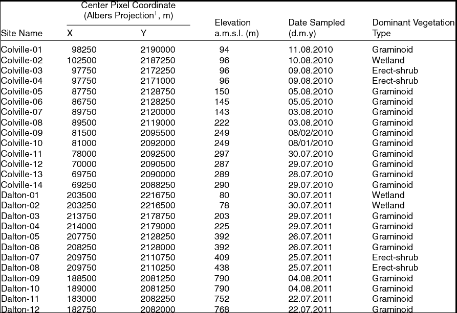
Sampling sites fell along an altitudinal and climatic gradient with the southernmost sites at higher elevation (~790 m) and influenced by the continental climate associated with the Brooks Range, while the northernmost sites were located at a much lower elevation (~73 m), where maritime climate conditions prevailed (Table 1). Sites along the Chandler and Colville rivers were located either in the floodplain or along tributary creeks within 1 km of the floodplain. In contrast, sites along the Dalton Highway were located at least 1 km away from the road to avoid the effect of road dust on the vegetation. Each sampling site was 250 m x 250 m for a total site area of 62,500 m2. This spatial resolution is adequate for regional studies as it corresponds to the spatial sampling of moderate resolution satellite imagers such as the Multi-angle Imaging SpectroRadiometer (MISR) and the Moderate Resolution Imaging Spectroradiometer (MODIS).
Description of Field Sites.
1 Coordinates are for an instance of the Albers Conical Equal Area map projection; see Duchesne and others Reference Duchesne, Chopping and Tape2015 for details and the map projection parameters used.
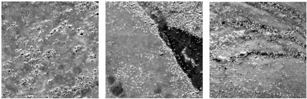
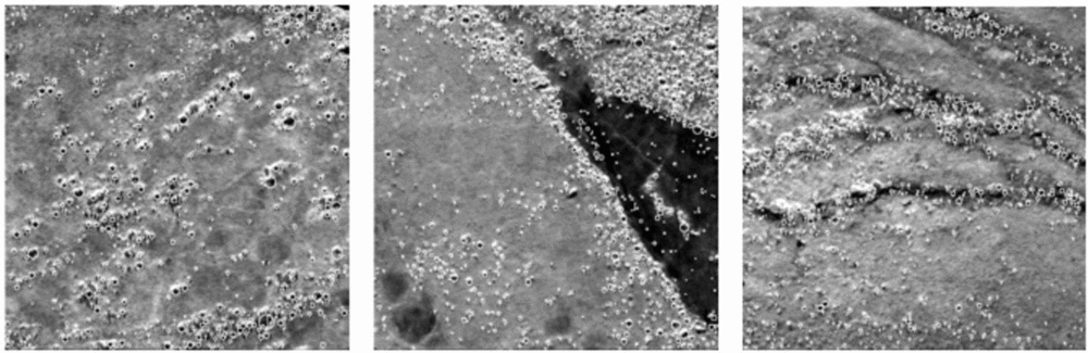
Field sites were selected using low-altitude aerial photographs and high-resolution satellite imagery (QuickBird, IKONOS, and WorldView). Selected sites represented a variety of tall shrub distributions, from dense willow shrubs (Salix spp.) and alder shrubs (Alnus viridis) along water tracks to scattered well-defined shrub canopies (Fig. 2). The location of the sites was mapped as graminoid-dominated tundra, erect-shrub-dominated tundra, and wetland (CAVM 2003), though riparian shrub sites are generally not represented in broad scale maps (Table 1). Graminoid tundra sites were typically dominated by sedges, dwarf shrubs less than 0.40 m tall, and a well-developed organic layer. There were often tall willow thickets (>2 m) occurring along stream margins. Erect-shrub tundra sites were characterised by low shrubs greater than 0.40 m tall. Wetland sites were dominated by sedges, grasses, and mosses. At most sites shrubs were less than 0.40 m tall; however, some sites hosted shrubs with an average height upwards of 1.5 m. Sites were sampled during the peak growing season when the shrub crown was at its fullest.
QuickBird panchromatic subsets with shrub crowns delineated by the CANAPI algorithm. Each site is 250 m x 250 m. From left to right: Colville-02, Colville-06, and Colville-10.
Target shrub population
The shrubs sampled were taller than 0.5 m. This height threshold was selected because it represents the approximate height boundary between shrubs that grow mainly between tussocks and shrubs that protrude above tussocks (Selkowitz Reference Selkowitz2010). The same threshold has also been widely used in other vegetation studies on the North Slope of Alaska to distinguish shrubs that form a canopy from background vegetation (Liston and others Reference Liston, Mcfadden and Sturm2002; Tape and others Reference Tape, Sturm and Racine2006). Canopy-forming shrubs play a different role in the ecosystem compared to inter-tussock shrubs. For instance, taller shrubs cast shadows on the background vegetation that in turn may change the micro-temperature around the shrub (Chapin and others Reference Chapin, Sturm and Serreze2005). They also trap more blowing snow during winter (Sturm and others Reference Sturm, Holmgren and Mcfadden2001a). In addition, taller shrubs can be more readily identified in very-high-resolution imagery, which allows the delineation of shrub crowns with greater ease.
Transect method and sampling strategy
The belt transect method was selected to obtain precise estimates of cover, height, and crown radius of shrub vegetation to compare with and assess the accuracy of the CANAPI algorithm. This is a common technique used to estimate the cover and height of woody vegetation, along environmental gradients, by extrapolating measurements within each belt transect to the entire sampling site (Hill and others Reference Hill, Fasham, Tucker, Shewry and Shaw2005). Since this can be a laborious technique it is recommended for sparse vegetation, as is the case of most tall shrub canopies in the Arctic. This method was used to survey all sites except Colville-01, where all shrubs were sampled.
The sampling strategy used to implement the belt transect method was systematic sampling with a randomly selected starting point. A baseline was placed along one side of the sampling sites and transects were laid perpendicular to the baseline. The first transect began at a randomly selected point along the baseline and transects thereafter were placed at regular intervals. In doing so, the sites were evenly sampled, the travel time and setup was reduced in comparison to random sampling, sampling units were better interspersed, and the same formulas inherent in simple random sampling were used (Elzinga and others Reference Elzinga, Salzer and Willoughby1998).
Two Garmin Etrex Geo-positional System (GPS), each with a horizontal accuracy of 10 m, were used to record the sampling transects and the location of each shrub surveyed. A Canon PowerShot digital camera was used to take photographs of all shrubs and a measuring rod was used to measure the height and crown width of each shrub.
Optimising field sampling
Prior to the field surveys, there were two important considerations: first, to decide on the most favorable transect width; and second, to determine the optimum number of transects to sample. From the statistical standpoint, long, narrow transects systematically placed (with a random start) in the population to be sampled are more effective for estimating cover than square or wider rectangular transects (Elzinga and others Reference Elzinga, Salzer and Willoughby1998). Therefore, the transects used were narrow rectangles of 250 m long by 5 m wide. Although a 6 m belt width is suggested when plant density is less than 15% (Tazik and others Reference Tazik, Warren and Diersing1992), which is the case for tall shrubs in Arctic tundra, a 5 m belt width still rendered reliable estimates of cover according to the pilot study.
A pilot study was carried out at site Colville-02 with the aid of QuickBird high-resolution panchromatic imagery (250 m x 250 m) and an image processing program (ImageJ) to determine the ideal number of transects to sample per site. Sequential sampling was used to determine the initial sample size using the transect method described above, in which the number of transects were increased monotonically from 3 to 15. With each iteration, the mean and standard deviation estimates were calculated. The sample size was plotted against the mean and standard deviation with the goal to identify the smallest sample size at which the curves began to smooth out. Finally, the mean and standard deviation values of the initial sample size were used to determine the ideal sample size for a site. This last process involved three steps (Elzinga and others Reference Elzinga, Salzer and Willoughby1998):
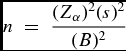
(1) calculating an uncorrected sample size estimate, n, by using equation 1:
 $$\begin{equation}
n\; = \;\frac{{(Z_\alpha )^2 (s)^2 }}{{(B)^2 }}\end{equation}$$
where n is the uncorrected sample size estimate, Zα is the standard normal coefficient, s is the standard deviation, and B is the desired precision level expressed as half of the maximum acceptable interval width.
(2) consulting the Sample Size Correction table to determine the corrected sample size estimate, n*. This was necessary because equation 1 underestimates the number of sampling units needed to meet the specified level of precision.
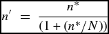
(3) multiplying the corrected sample size estimate by the finite population correction factor when more than 5% of the population is being sampled using equation 2:
 $$\begin{equation}
n'\; = \;\frac{{n^{*}}}{{(1 + (n^{*}/N))}}\end{equation}$$
where nʹ is the new FPC-corrected sample size, n* is the corrected sample size from the Sample Size Correction table, and N is the total number of possible transect locations in the population. N is calculated by dividing the total area of the population by the size of one transect (N = 62500 m / 1250 m = 50).
Sampling shrub parameters
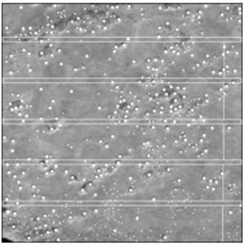
The four corners of the sampling site were located in the field using GPS. A baseline parallel to the terrain slope was laid along one of the sides of the site. The starting point of the first transect was randomly located within the first 50 m of the baseline and established perpendicular to it. The subsequent transects were located parallel to the first and equally spaced from each other (Fig. 3).
Distribution of belt transects at site Colville-02 (250 m x 250 m) following a systematic sampling strategy with a randomly selected starting point. White dots represent shrubs observed in the QuickBird panchromatic image.
Three people did the sampling. The first person walked the transect using a GPS to mark the path with flags. The second person walked along the transect with a 5 m pole held horizontally (2.5 m on each side of the transect), stopping at every shrub taller than 0.5 m that had at least half of its base located within the belt. The third person recorded the GPS location of the shrub and took a picture of it next to a 2 m scale rod (with 0.10 m increment marks). The process was repeated until all shrubs within the belt and all transects at a site were sampled.
Shrub genus was identified later using the photographic records and field notes. Photographs were also used to estimate canopy width (horizontal extent from the left-most branch to the right-most branch) and height (vertical extent from base to top of foliage) of the shrubs by calibrating distances in the photo using the 2 m scale rod placed beside each shrub.
Deriving shrub site parameters using belt transects
The belt transect method was used to determine fractional cover, total number of shrubs, shrub mean crown radius, and mean shrub height at each site. Mean crown radius was estimated using all measurements of individual shrubs, including those where crown diameter exceeded the 5 m belt width. Clusters of shrubs were omitted from the analysis because the crown borders of each shrub could not be identified. Mean crown radius was defined as half of the mean crown diameter. Mean shrub height was estimated using all the observations, both individual shrubs and clusters of shrubs. Shrub height was defined as the length of the shrub from its base to the top branch. Fractional cover estimates included both surveyed individual shrubs and clusters of shrubs. The crowns that exceeded the belt width were adjusted to 5 m. Estimation of fractional cover was a two-step process:
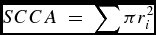
(1) Estimation of shrub/cluster cover area (SCCA), which assumes that the canopy was round:
 $$\begin{equation}
SCCA\; = \;\sum \pi r_i ^2\end{equation}$$
where ri is the individual shrub or shrub cluster crown radius (m),
(2) Estimation of fractional cover (FC):
 $$\begin{equation}
FC\; = \;SCCA/TBA\end{equation}$$
where SCCA is shrub cover area (m2) and TBA is the sum of the area covered by all belt transects sampled at a site (1250 m2/transect). Fractional cover values range from 0 to 1, with 1 being 100% shrub cover.
Total number of shrubs (TNS) in the sampling site was estimated using records of individual and cluster of shrubs where each shrub or shrub cluster was considered one individual:
 $$\begin{equation}
TNS\; = \;A*S/TBA\end{equation}$$
where A is the site area (62,500 m2), and S is the total number of shrubs and clusters surveyed in all belt transects.
CANAPI estimates and calibration equations
CANAPI is a user-adjustable algorithm that can be run in ImageJ and uses high-resolution panchromatic imagery to analyse tree and shrub canopies (Chopping Reference Chopping2011). The CANAPI algorithm operates in two steps: first, it identifies crowns by locating the crescent-shaped sunlit portion of the crown; and second, it attempts to estimate tree or shrub height using the length of the shadow cast by each crown, where the shadow is not truncated by another crown or the edge of the image. For application in Arctic tundra, CANAPI's parameters and filter settings were adjusted for each site separately, until the number of crowns delineated by CANAPI roughly matched those observed in the high-resolution imagery.
The CANAPI algorithm was used here to derive fractional shrub cover, canopy crown radius, total number of shrubs, and shrub height estimates for the field sites (Fig. 2). The CANAPI algorithm estimates were derived from image subsets of 250 m x 250 m, corresponding to the field sites, aligned with the Albers Equal Area Conic grid, selected from sub-meter high-resolution panchromatic scenes from the QuickBird, WorldView, and GeoEye sensors (0.6 m, 0.5m, and 0.5 m spatial resolution, respectively). Some imagery was purchased, while some was obtained through the National Geospatial-Intelligence Agency Commercial Archive Data (http://cad4nasa.gsfc.nasa.gov/). Field data were considered to be more reliable than CANAPI estimates because shrubs were measured in situ. Thus, field data were used to validate image-based estimates of fractional cover, mean crown radius, mean height, and total number of shrubs via regression equations.
Sites with indiscrete shrubs were not suitable for the CANAPI algorithm and were not included in the regression analysis. CANAPI requires shrub crowns to be well defined in order to identify them in the high-resolution satellite imagery. Four CANAPI estimates of fractional cover were omitted from the analysis because at those sites shrubs formed a homogeneous layer that made it impossible to delineate shrub crowns. Similarly, five CANAPI estimates of total shrub were excluded from the analysis because of the homogeneous layer of shrubs (4 sites) and almost leafless shrub crowns (1 site). Two CANAPI estimates of mean crown radius were not included in the analysis because at those sites there was either no shrub surveyed in the field or detected by CANAPI. Three CANAPI estimates of mean shrub height were omitted from the analysis because at one site there were no shrubs surveyed in the field, and at the other two sites the few shrubs detected by CANAPI had their shadows truncated by other shrubs.
Results and discussion
Optimising field sampling
The mean number of shrubs and standard deviation values became rather stable once at least nine transects were sampled (mean = 10.3, SD = 2.29). According to equation 1, the uncorrected sample size estimate (n) should be 1 (Zα = 1.64, B = 3.8). Consistent with the Sample Size Correction table, the corrected sample size estimate for a 90% confidence interval should be 5 (n* = 5). Since sampling five belts (6,250 m2) means sampling more than 5% of the area (62,500 m2), the correction to a sample size estimate that incorporates the finite population correction (FPC) factor was applied. A minimum of five transects were required to be 90% confident that the estimate of the population mean was within +/- 4 shrubs of the true mean.
Sampling shrub parameters
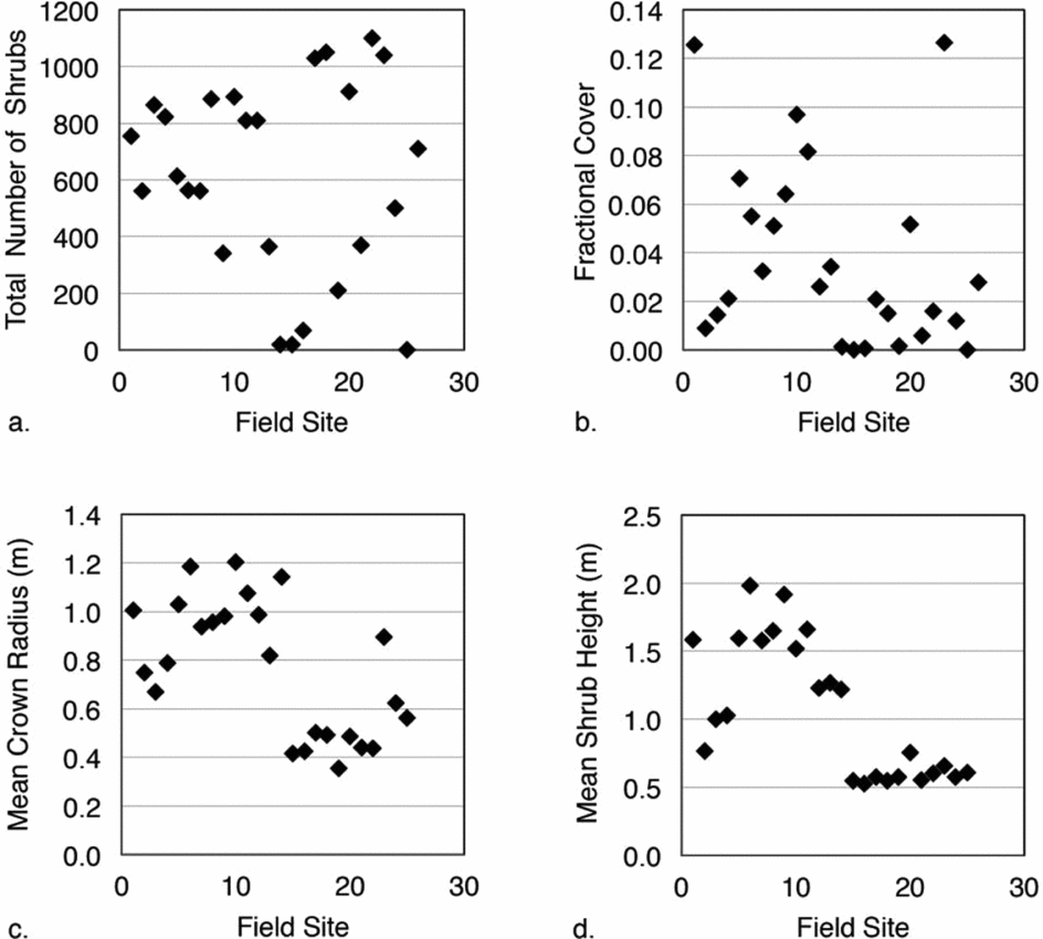
The total number of shrubs taller than 0.5 m ranged from 0 to 1520 at the 26 field sites (Fig. 4a). Fractional cover estimates varied from 0.00 to 0.13 or 0 to 13% at the sampling sites (Fig. 4b). The mean crown radius estimates ranged from 0.36 m to 1.21 m, while the maximum mean shrub height was 1.98 m (Figs. 4c, 4d, respectively). About 0.2 m of the shrubs’ height is usually hidden between tussocks. Alder was the dominant shrub at 13 out of the 26 sites sampled (percentage dominance > 67%), while willow was the dominant shrub at 12 sites (percentage dominance > 53%). At site Dalton-09 there were no shrubs.
Shrub structural estimates at the 26 sampling sites: (a) total number of shrubs, (b) fractional cover, (c) mean crown radius, and (d) mean shrub height.
CANAPI estimates and calibration equations
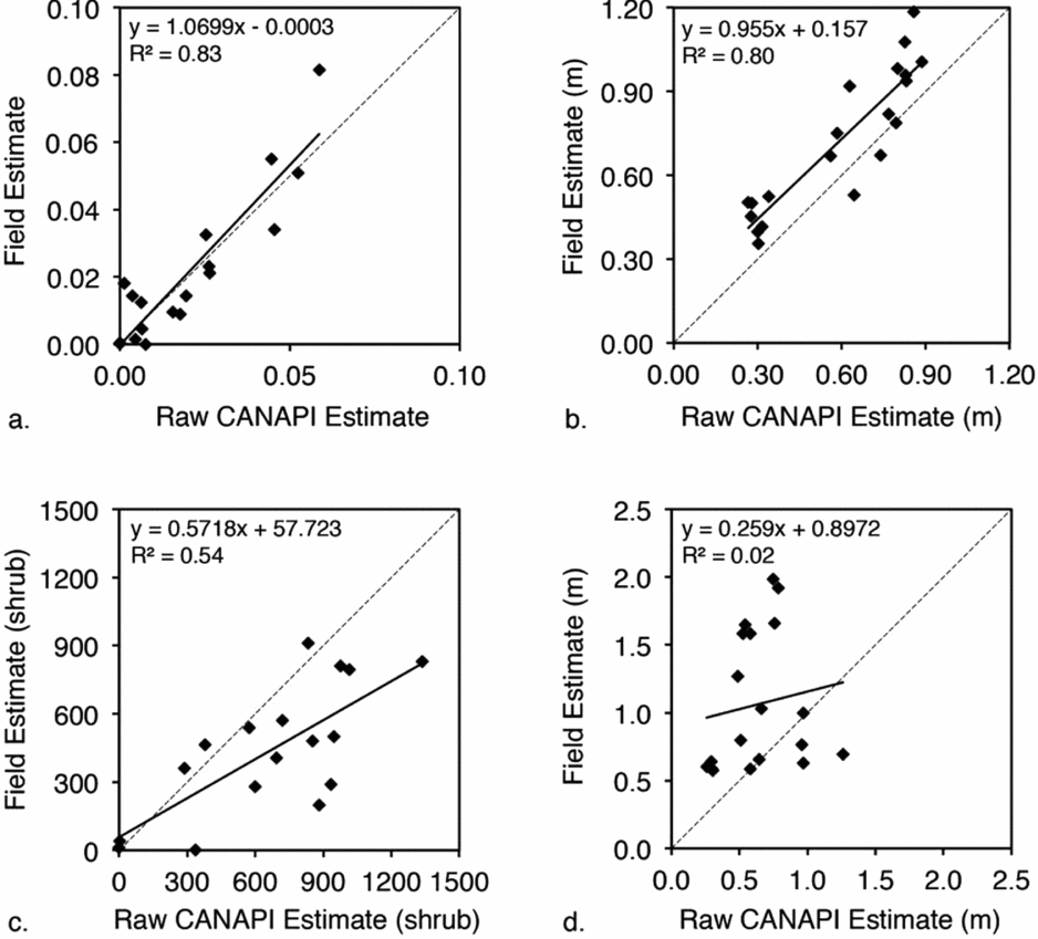
Regression lines between field and CANAPI estimates for four vegetation structural variables were estimated. The coefficients of determination for fractional cover and mean crown radius revealed a strong positive relationship between field and CANAPI estimates (R2 = 0.83 and 0.80, respectively; RMSE = 0.009 and 0.17 m, respectively; P < 0.001) (Figs. 5a, 5b). The relationship between field and CANAPI estimates for the total number of shrubs was also positive but not as strong (R2 = 0.54, RMSE = 334 shrubs, P < 0.001) (Fig. 5c). The correlation between field and CANAPI estimates for shrub height was not significant (R2 > = 0.02, RMSE = 0.67 m, P = 0.57) (Fig. 5d).
Correlations between ‘raw’ CANAPI estimates and field estimates for four vegetation structural variables: (a) fractional cover (P < 0.001), (b) mean crown radius (P < 0.001), (c) total number of shrubs (P < 0.001), and (d) mean height (P = 0.57).
Further exploration of these relationships revealed that CANAPI tended to underestimate fractional cover when there were clusters of shrubs, because CANAPI was unable to identify the shrub crowns in the cluster. Wherever vegetation was sparse, CANAPI estimates were consistent with field data because CANAPI could identify the individual shrub crowns. Similar relationships applied to the estimates of the total number of shrubs. Mean crown radius CANAPI estimates were often lower than the corresponding field estimates. This might also be an effect of the coarse spatial resolution of the panchromatic images used to derive the CANAPI estimates in comparison to the finely resolved field measurements.
The CANAPI mean shrub height estimates tended to be lower than the field values, but there was not a clear pattern, resulting in a poor coefficient of determination. CANAPI predicts the height of an object by measuring the length of the shadow cast and by multiplying it by the tangent of the sun elevation angle. This means that there are at least three sources of error that may account for the differences between the field and CANAPI estimates: 1) the coarse spatial resolution of the sensors compared to the precise measurements made in the field; 2) different sensor-object geometries from the different high-resolution sensors used (QuickBird, GeoEye, WorldView 1 and 2) that were not accounted for by the CANAPI algorithm; and 3) error from field measurements and subsequent calculations, though this is considered a much smaller term.
The high coefficient of determination values for fractional cover and mean crown radius (0.83 and 0.80 respectively) suggests that it is appropriate to use the regression coefficients to adjust shrub CANAPI estimates in Arctic tundra (Equations 6 and 7). Although the coefficient of determination was not low for total number of shrubs (0.53), the regression coefficients must be used with caution (Equation 8). It is not recommended that the regression equation be used to adjust CANAPI estimates of mean shrub height due to the poor correlation found with the field estimates.
 $$\begin{eqnarray}
{\rm Fractional\ cover}\;&{\rm = }&\;{\rm (1}{\rm .0699}\;{\rm x}\;{\rm CANAPI\ estimate)}\;\nonumber\\
&&{\rm - }\;{\rm 0}{\rm .0003}\end{eqnarray}$$
 $$\begin{eqnarray}
{\rm Mean\ crown\ radius}\;&{\rm = }&\;{\rm (0}{\rm .955}\;{\rm x}\;{\rm CANAPI}\;{\rm estimate)}\;\nonumber\\
&&{\rm + }\;{\rm 0}{\rm .157}\end{eqnarray}$$
 $$\begin{eqnarray}
{\rm Shrub\ total}\;{\rm = }\;{\rm (0}{\rm .5718}\;{\rm x}\;{\rm CANAPI}\;{\rm estimate)}\;{\rm + }\;{\rm 57}{\rm .723}\nonumber\\
\end{eqnarray}$$
The CANAPI algorithm is sensitive to small changes in woody vegetation cover and consistently detects a wide size range of erect shrubs. The sensitivity of the algorithm is a key factor given that at a spatial resolution of 250 m tall shrub cover is usually less than 5% in the Arctic (Beck and others Reference Beck, Horning and Goetz2011; Selkowitz Reference Selkowitz2010). Results showed that when adjusting the algorithm's parameters and filter settings for each site, CANAPI can provide good estimates of fractional cover, crown radius, and total number of shrubs with remarkable confidence in spite of the important limiting factors: 1) the surrounding background is composed of mixed vegetation (tussocks, moss, and lichens), and therefore there is less contrast between shrubs and their background; 2) the signal is quite small since 75 percent of the time cover is less than 0.02 in the Arctic landscape at 250 m scales; and 3) shrubs are considerably smaller than trees (the target population where CANAPI has been previously used successfully) and thus more difficult to detect.
Conclusions
CANAPI is a user friendly, user-adjustable algorithm that can perform well under different scenarios, in particular, with sparse woody vegetation. The results obtained in this study show that CANAPI provides a way to build reference datasets for some important structural characteristics of the woody vegetation directly from high-resolution panchromatic imagery. CANAPI provides data that can be used to assess the results of other mapping or estimation approaches, though the regression equations developed here for Arctic Alaska will apply most accurately in similar tundra landscapes. A comprehensive data set ‘Woody Vegetation Characteristics of 1,039 Sites across the North Slope, Alaska’ was derived in this way by a NASA Terrestrial Ecology Program project for the North American Carbon Program (NACP; Wofsy and Harriss Reference Wofsy and Harriss2002) and has been made available at the Oak Ridge National Laboratory (ORNL) Distributed Active Archive Center (DAAC) (Duchesne and others Reference Duchesne, Chopping and Tape2015). A copy of the CANAPI algorithm is included along with shrub canopy statistics for 26 field sites that might be useful if adjustment of the equations is desired in order to help account for user bias. Future research projects and campaigns such as the upcoming NASA-sponsored Arctic-Boreal Vulnerability Experiment (ABoVE; Kasischke and others Reference Kasischke, Goetz, Kimball and Mack2010) that require data on shrub abundance in Arctic tundra may opt to use the NACP database. For example it could be used to assess the results of ABoVE remote sensing initiatives that attempt to exploit imagery acquired at lower spatial resolutions (for example from Landsat, or NASA's Multi-angle Imaging SpectroRadiometer (MISR) and Moderate Resolution Imaging Spectroradiometer (MODIS)); or by using CANAPI with earlier and/or more current imagery to assess changes in cover through time.
Acknowledgments
We thank the National Geospatial-Intelligence Agency (NGA) for providing high-resolution imagery (cad4nasa.gsfc.nasa.gov). Thanks to field assistants Jesse Carlstrom, Michael Cohrs, and Scott Buchanan, who participated in the field surveys. This work was supported by the National Aeronautics and Space Administration (award NNX09AL03G to M.J.C.); and the Geological Society of America (Graduate Student Research grant to R.R.D.)