1 Introduction
Membranes are commonly used in industry, since their functions span from desalination to recovery of precious metals passing through sterile filtration, food processing, paint and solvent recovery, petroleum refining and other industrial, medical and environmental applications (cf. Mohanty & Purkait (Reference Mohanty and Purkait2011), for a review, or Song et al. (Reference Song, Stone, Jensen and Lee2019) for a recent example on deformable polydimethylsiloxane membranes). They are also important in nature, since plants depend heavily on osmosis and filtration for their water and sugar translocation (cf. for instance, Jensen et al. (Reference Jensen, Berg-Sørensen, Bruus, Holbrook, Liesche, Schulz, Zwieniecki and Bohr2016)). Each function is associated with a specific pore dimension, ranging from  $10~\unicode[STIX]{x03BC}\text{m}$ to 1 mm for particle filtration (able to filter human air, fat micelles and activate carbons) to 1 nm for the osmosis used in desalination (Fritzmann et al. Reference Fritzmann, Lowenberg, Wintgens and Melin2007; Elimelech & Phillip Reference Elimelech and Phillip2011; Matin et al. Reference Matin, Khan, Zaidia and Boyce2011) and in wastewater recovery (Shannon et al. Reference Shannon, Bohn, Elimelech, Georgiadis, Mariñas and Mayes2008; Rahardianto, McCool & Cohen Reference Rahardianto, McCool and Cohen2010), with intermediate steps for microfiltration, ultrafiltration and nanofiltration (cf. Rautenbach & Albrecht Reference Rautenbach and Albrecht1994). Since separation processes constitute
 $10\,\%\sim 15\,\%$ of the world energy consumption (Sholl & Lively Reference Sholl and Lively2016), Park et al. (Reference Park, Kamcev, Robeson, Elimelech and Freeman2017) highlighted recently the need for a better understanding of the mechanisms behind these processes, responsible of the trade-off between permeability and selectivity of membranes, in order to exceed the existing bounds and reduce energy consumption.
Analysed from a geometrical point of view, membranes are porous media where the characteristic size of the pores is much smaller than that of the bulk along the filtration direction (called here traditional or thick membranes). If we assume instead that the macroscopic characteristic size along the filtration direction is of the order of the pore size or smaller, we deal with thin membranes, which may represent a strategy to decrease the energy used during filtration. Thanks to the successful synthesis of graphene by Novoselov et al. (Reference Novoselov, Geim, Morozov, Jiang, Zhang, Dubonos, Grigorieva and Firsov2004), it is nowadays possible to build quasi-two-dimensional permeable surfaces and, following this path, many patents based on ultra-thin membranes have been created (cf. for instance, Karan, Jiang & Livingston (Reference Karan, Jiang and Livingston2015)). One of the critical points in membrane design is to combine mechanical resistance to stresses with a determined permeability and selectivity. When particles encounter a membrane, if their mass is too high, a rupture of the membrane may happen. Moreover, to address issues related to fouling (the deposition of particles’ solute on the membrane surface), one of the principal origins of the decrease of membrane performance (Bucs et al. Reference Bucs, Valladares Linares, Vrouwenvelder and Picioreanu2016), some strategies have been developed, such as pressure driven backwashing either in micro- ultra- and nano-filtration, (cf. for instance Roh, Kim & Park (Reference Roh, Kim and Park2002), Ramon, Agnon & Dosoretz (Reference Ramon, Agnon and Dosoretz2010)). In this procedure, high pressure gradients act on the membrane, causing a possible breach. Many works with the purpose of reinforcing membranes via the use of layers of crossed fibres have been proposed, mostly experimental in nature, as in Chou, Wang & Fane (Reference Chou, Wang and Fane2013) and She et al. (Reference She, Wei, Ma, Sim, Fane, Wang and Tang2016), without identifying a systematic criterion to tackle these issues.
Hence, processes involving membranes still present many open questions which a rigorous monolithic approach could help to clarify. However, an analysis of the literature on membrane technologies shows that experimental works are more common than theoretical and numerical studies and the molecular, chemical, biological point of view is preferred to a continuum fluid mechanics approach (cf. for instance, Farahbakhsh, Delnavaz & Vatanpour (Reference Farahbakhsh, Delnavaz and Vatanpour2017)). Studies aiming at describing the behaviour of fluid flows through traditional thick membranes, from a full continuum point of view, are generally based on the early works of Kedem and collaborators, such as Kedem & Katchalsky (Reference Kedem and Katchalsky1958) and Spiegler & Kedem (Reference Spiegler and Kedem1966). In these works, since thick membranes are essentially porous media, the equations describing the fluid flows through membranes resemble Darcy’s law (Darcy Reference Darcy1856), with an added pressure gradient which depends on different distributions of the solute across the membrane. In these equations, ad hoc tuned parameters appear, such as the permeability associated with the fluid and with the solute, often deduced with the use of experimental laws (see Bacchin (Reference Bacchin2017), for a recent example). Cardoso & Cartwright (Reference Cardoso and Cartwright2014) tried to include in the same continuum model a microscopic characterization of the solvent–solute behaviour via the introduction of a parameter found by solving problems at molecular scale. A further step has been done by Ledesma-Duran, Hernández & Santamaría-Holek (Reference Ledesma-Duran, Hernández and Santamaría-Holek2016, Reference Ledesma-Duran, Hernández and Santamaría-Holek2017), assuming the validity of a set of continuum equations taken from different theories, they find a strategy to characterize the intrinsic parameters related to the triple solvent–solute–membrane by solving pore-scale problems for some specific geometries. Despite the fact that the membrane community is focussed on the chemical aspects of the phenomenon more than the mechanics of the fluids flowing through the membranes, a rigorous alternative to developing theoretical models to simulate the flow field across porous media can be found in upscaling techniques like the volume averaging method (Whitaker Reference Whitaker1998) and multiscale homogenization theory (Hornung Reference Hornung1997). Early works carried out using these techniques were focussed on the development of a model for fluids flowing within unbounded porous media and confirmed the validity of Darcy’s law under certain flow conditions. More recent developments have shown that a rigorous treatment of interfaces between porous regions and free fluid regions is possible, with either volume averaging (Ochoa-Tapia & Whitaker Reference Ochoa-Tapia and Whitaker1995; Valdés-Parada et al. Reference Valdés-Parada, Aguilar-Madera, Ochoa-Tapia and Goyeau2013; Pasquier, Quintard & Davit Reference Pasquier, Quintard and Davit2017) or homogenization (Carraro et al. Reference Carraro, Goll, Marciniak-Czochra and Mikelić2015; Lācis & Bagheri Reference Lācis and Bagheri2017). These techniques are not solely limited to quantifying the momentum transfer across interfaces, but enable also the study of mass transfer, including chemical reactions between different species (Veran, Aspa & Quintard Reference Veran, Aspa and Quintard2009). While the theory for porous media is suitable to model fluid flows across thick membranes, this is not the case for thin membranes, whose literature is more limited (Malone, Hutchinson & Prager Reference Malone, Hutchinson and Prager1974; Brunn Reference Brunn1984; Jiang, Karan & Livingston Reference Jiang, Karan and Livingston2018). In these works, Darcy’s law is assumed to be valid across the membrane, i.e.
 $$\begin{eqnarray}\boldsymbol{u}=-\boldsymbol{K}\unicode[STIX]{x1D735}p,\end{eqnarray}$$
where  $\boldsymbol{u}$ is the velocity at the membrane,
 $\boldsymbol{K}$ the permeability and
 $\unicode[STIX]{x1D735}p$ the pressure gradient across the membrane. The crucial point to formally justify the averaged equation above via upscaling techniques is that the pressure loss across the membrane occurs over a macroscopic length scale
 $L$. Considering Stokes’ equations within the near membrane zone and writing the balance between the pressure gradient and the viscous dissipation (occurring at a microscopic scale
 $l$ such that
 $\unicode[STIX]{x1D716}=l/L\ll 1$) we obtain that the pressure jump scales like
 $\unicode[STIX]{x0394}P=\unicode[STIX]{x1D716}^{-1}(\unicode[STIX]{x1D707}U/l)$ and, hence, is dominant. This allows one to write the velocity as in (1.1). Conversely, with thin membranes, the pressure loss occurs on the microscopic scale
 $l$ and the pressure jump scales like
 $\unicode[STIX]{x0394}P=\unicode[STIX]{x1D707}U/l$, being no more dominant in Stokes’ equation, rendering unjustified the assumption of Darcy’s law. In other words, Malone et al. (Reference Malone, Hutchinson and Prager1974), Brunn (Reference Brunn1984) and Jiang et al. (Reference Jiang, Karan and Livingston2018) essentially show that, if a model based on the concept of a permeability is chosen to simulate the macroscopic flow through thin membranes, the way to compute the permeability must be modified and it obeys different laws with respect to the case of thick membranes. In a recent paper, Melnikov, Hulings & Gracheva (Reference Melnikov, Hulings and Gracheva2017) have shown that the fluid velocity profile through thin pores, found via direct numerical simulations, is completely different from that expected from the theory valid for thick pores.
Some works (Conca Reference Conca1987a,Reference Concab; Bourgeat, Marusic & Marusic-Paloka Reference Bourgeat, Marusic and Marusic-Paloka1997; Bourgeat & Marusic-Paloka Reference Bourgeat and Marusic-Paloka1998; Bourgeat, Gipouloux & Marusic-Paloka Reference Bourgeat, Gipouloux and Marusic-Paloka2001) have been devoted to the mathematical formal analysis of incompressible fluid flows through thin membranes, with a focus on specific flow configurations such as flow purely normal to the membrane. Other works (cf. for instance, Tio & Sadhal (Reference Tio and Sadhal1994), Wang (Reference Wang1994), Jensen, André & Stone (Reference Jensen, André and Stone2014)) propose analytical solutions of the flow for very specific and rather simplified geometries of the structured permeable surface, without enabling a generalization to more complex or realistic geometrical configurations.
The present work aims to provide a continuum model for fluid flows across thin membranes, for the most general flow configuration, microscopic geometry and macroscopic membrane shape, starting from two simple considerations: Macroscopically, a thin membrane is essentially an interface which splits a fluid domain into two regions, and its presence can be simulated by simply changing the fluid effective properties at that interface. Microscopically, a membrane has a peculiar, specific structure and the topological characteristics of this structure influence the macroscopic flow behaviour, hence, a way to upscale the properties from the microscale to the macroscale has to be found. A standard homogenization method (Mei & Vernescu Reference Mei and Vernescu2010), modified as in Jiménez Bolaños & Vernescu (Reference Jiménez Bolaños and Vernescu2017) and Zampogna, Magnaudet & Bottaro (Reference Zampogna, Magnaudet and Bottaro2019) to deal with interfaces, is the key point to efficiently perform the required upscaling. The modifications (whose mathematical foundations can be found also in Achdou et al. Reference Achdou, Le Tallec, Valentin and Pironneau1998a; Achdou, Pironneau & Valentin Reference Achdou, Pironneau and Valentin1998b; Mohammadi, Pironneau & Valentin Reference Mohammadi, Pironneau and Valentin1998) are essentially based on a decomposition of the full-scale flow in an outer part, independent of the microscale, and a inner part, depending on the microscale, which has been formally introduced in the homogenization framework by Lācis & Bagheri (Reference Lācis and Bagheri2017) and further developed in Lācis et al. (Reference Lācis, Sudhakar, Pasche and Bagheri2020) and Sudhakar et al. (Reference Sudhakar, Lācis, Pasche and Bagheri2019). In § 2 we introduce the macroscopic model with the minimal definitions needed by the reader to understand the jump conditions. A physical interpretation of the model is given, which suggests generalizing the concept of permeability, which remains valid for special flow and membrane configurations. As a consequence, two more general entities, the upward and downward Navier tensors, are introduced. In § 3 its development is explained; we analyse the inner flow using homogenization and deduce boundary conditions for the microscopic problems from the flow in the region far from the membrane. Once the model is found, the solution procedure requires two steps; in the first instance, problems at the microscale have to be solved in order to find the effective properties of the membrane, represented by the upward and downward Navier tensors (§ 4.1). These effective properties are used, in a second instance, to find the macroscopic solution, which has been computed in § 4.2 for different test cases. The model is validated by systematic comparisons with direct numerical simulations of the fluid flow across the thin membrane. Finally, in § 5 we summarize the main findings of the paper and we discuss the impact of the new model on the present literature and its future development.
2 An equivalent condition for thin permeable walls
As stated in the introduction, the objective of the present work is to deduce an equivalent condition for a fluid flow encountering a microstructured permeable thin wall. The equivalent condition, purely macroscopic, is a constraint jump within the fluid domain, imposed at a fictitious surface which is placed in the middle of the real permeable wall. This condition contains information about the microscopic structure of the wall analysed, allowing us to evaluate the macroscopic consequences due to changes at the microscopic level.
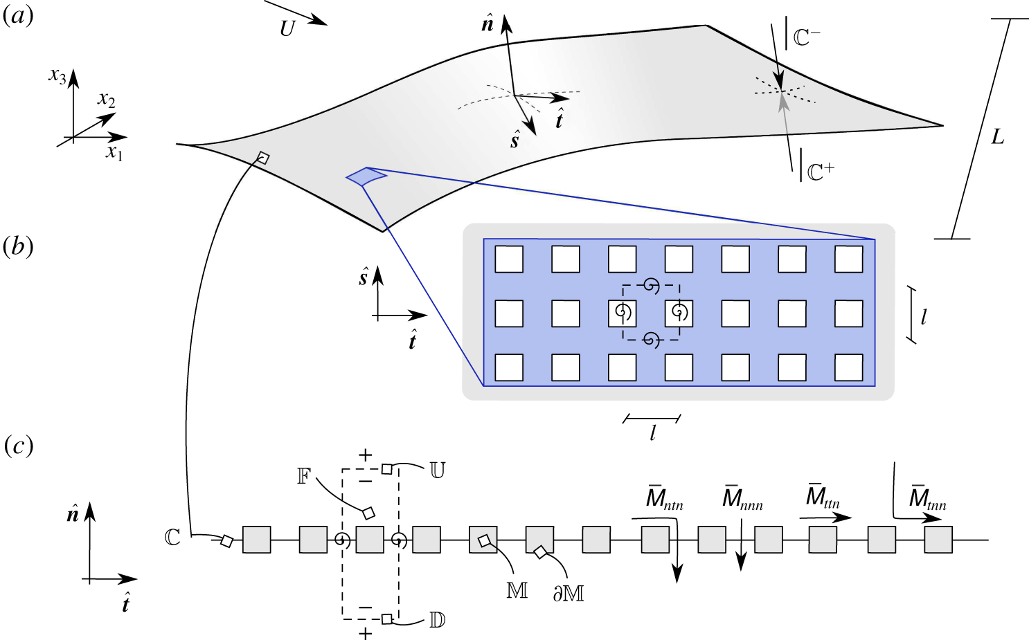
Fluid flow encountering a thin permeable membrane. (a) From a macroscopic point of view the micro-perforated surface corresponds to a fictitious wall denoted with  $\mathbb{C}$, provided with a local frame of reference
 $(\hat{\boldsymbol{s}},\hat{\boldsymbol{t}},\hat{\boldsymbol{n}})$. We define the upward side of the membrane as the side of
 $\mathbb{C}$ whose outer normal coincides with
 $\hat{\boldsymbol{n}}$ in the sketch, counter-imposed on the downward opposite side. Its size along the tangential directions
 $\hat{\boldsymbol{s}}$ and
 $\hat{\boldsymbol{t}}$ is of order
 $L$. (b) Zoom in on the plane
 $(\hat{\boldsymbol{s}},\hat{\boldsymbol{t}})$ of the blue portion of
 $\mathbb{C}$ in (a). The pores form a periodic pattern realized by the repetition of the microscopic cell represented by the dashed square. The cell size along
 $\hat{\boldsymbol{s}}$ and
 $\hat{\boldsymbol{t}}$ identifies the microscopic length scale
 $l$. (c) Projection on the plane
 $(\hat{\boldsymbol{t}},\hat{\boldsymbol{n}})$ of a portion of the membrane. The aspect ratio between the tangential and normal sizes of the solid inclusions is set equal to 1. Along
 $\hat{\boldsymbol{s}}$ and
 $\hat{\boldsymbol{t}}$ the flow is periodic while on
 $\mathbb{U}$ and
 $\mathbb{D}$ (respectively the upward and downward sides of the cell) we impose the conditions in (2.5). Some relevant components of the upward Navier tensor
 $\bar{\unicode[STIX]{x1D648}}$ (cf. (2.6)) are visualized in local curvilinear coordinates:
 $\bar{\unicode[STIX]{x1D614}}_{nnn}$ and
 $\bar{\unicode[STIX]{x1D614}}_{ttn}$ contribute respectively to the purely normal and tangential fluid motions near the membrane while
 $\bar{\unicode[STIX]{x1D614}}_{tnn}$ is linked to the tangential component of the normal fluid motion and
 $\bar{\unicode[STIX]{x1D614}}_{ntn}$ to the normal component of the tangential fluid motion.

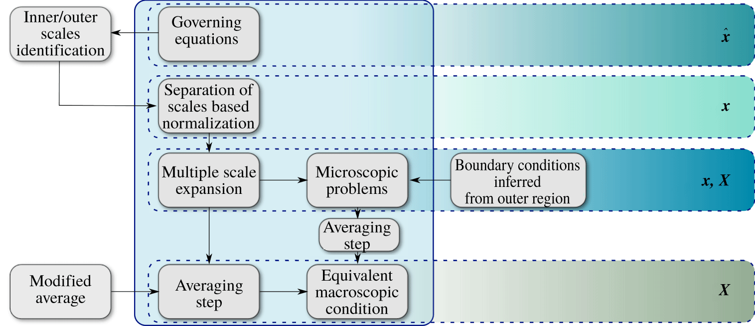
Diagram of the procedure used to deduce condition (2.6). In the solid edged big rectangle the main steps of a standard homogenization technique are listed. The remaining steps have been added to render the standard procedure suitable to analyse flows through thin permeable surfaces. On the right, for each step, the different kinds of spatial variables present are highlighted:  $\hat{\boldsymbol{x}}$ denotes the dimensional spatial variable while
 $\boldsymbol{x}$ and
 $\boldsymbol{X}$ the microscopic and macroscopic non-dimensional spatial variables, which scale with
 $l$ and
 $L$, respectively.

In this section the macroscopic model is introduced and explained from a physical point of view, while the mathematical procedure to obtain the model is described in § 3. We consider an incompressible Newtonian fluid of constant density  $\unicode[STIX]{x1D70C}$ and viscosity
 $\unicode[STIX]{x1D707}$, encountering a rigid perforated wall, from now on a membrane
 $\mathbb{M}$, as sketched in figure 1. The dimensional velocity
 $\hat{u} _{i}$ and pressure
 $\hat{p}$ in the fluid domain
 $\mathbb{F}$ (cf. figure 1) are governed by the Navier–Stokes equations
 $$\begin{eqnarray}\displaystyle & \displaystyle \unicode[STIX]{x1D70C}\hat{\unicode[STIX]{x2202}}_{t}\hat{u} _{i}+\unicode[STIX]{x1D70C}\hat{u} _{j}\hat{\unicode[STIX]{x2202}}_{j}\hat{u} _{i}=-\hat{\unicode[STIX]{x2202}}_{i}\hat{p}+\unicode[STIX]{x1D707}\hat{\unicode[STIX]{x2202}}_{ll}^{2}\hat{u} _{i}, & \displaystyle\end{eqnarray}$$
 $$\begin{eqnarray}\displaystyle & \displaystyle \hat{\unicode[STIX]{x2202}}_{i}\hat{u} _{i}=0, & \displaystyle\end{eqnarray}$$
with  $\hat{u} _{i}=0$ on the solid–fluid boundary
 $\unicode[STIX]{x2202}\mathbb{M}$. The membrane geometry allows us to identify two different characteristic lengths: the macroscale
 $L$ of the large-scale flow structures, which in figure 1 coincides with the extension of the entire membrane, along
 $\hat{\boldsymbol{s}}$ and
 $\hat{\boldsymbol{t}}$, and the microscale
 $l$, characterizing the pores and the thickness of the membrane, introduced in figure 1(b). The ratio between
 $l$ and
 $L$ defines a suitable separation of scales parameter,
 $\unicode[STIX]{x1D716}$, such that
 $$\begin{eqnarray}\unicode[STIX]{x1D716}:=\frac{l}{L}\ll 1.\end{eqnarray}$$
The membrane is formed by a periodic repetition of the microscopic elementary cell, the cuboid represented as two dashed rectangles in figure 1(b) and (c). Within this cell, the flow field is supposed to be periodic along the tangential-to-the-surface directions  $\hat{\boldsymbol{s}}$ and
 $\hat{\boldsymbol{t}}$. The ensemble of microscopic cells covers the whole surface and identifies the inner region, as opposed to the outer region, composed of the remaining fluid domain. The fluid flow scales in different ways in these regions; in the inner region it depends on the micro- and the macroscale while in the outer region it depends only on the macroscale. We define the upward region as the portion of fluid domain adjacent to the side of
 $\mathbb{C}$ whose outer normal coincides with
 $\hat{\boldsymbol{n}}$, counter-imposed on the downward region on the opposite side. Across the upward and downward boundaries of the microscopic cell,
 $\mathbb{U}$ and
 $\mathbb{D}$, continuity of velocities and tractions is valid, i.e.
 $$\begin{eqnarray}\hat{u} _{i}^{-}=\hat{u} _{i}^{+}\end{eqnarray}$$
and
 $$\begin{eqnarray}\hat{\unicode[STIX]{x1D6F4}}_{jk}^{-}n_{k}=\hat{\unicode[STIX]{x1D6F4}}_{jk}^{+}n_{k},\end{eqnarray}$$
where the superscripts  $^{+}$ and
 $^{-}$ above the velocity and the stress tensor
 $\hat{\unicode[STIX]{x1D6F4}}_{jk}=\hat{p}\unicode[STIX]{x1D6FF}_{jk}+2\unicode[STIX]{x1D707}\hat{\unicode[STIX]{x1D716}}_{jk}(\hat{\boldsymbol{u}})$, specify that we are considering the
 $-$ or
 $+$ sides of
 $\mathbb{U}$ and
 $\mathbb{D}$, according to the notation in figure 1(c). The tensor
 $\hat{\unicode[STIX]{x1D716}}_{jk}$ denotes the strain, i.e.
 $\hat{\unicode[STIX]{x1D716}}_{jk}=\frac{1}{2}(\hat{\unicode[STIX]{x2202}}_{j}\hat{u} _{k}+\hat{\unicode[STIX]{x2202}}_{k}\hat{u} _{j})$. Interface condition (2.5) will be used later on to couple the inner and outer flows. The fictitious surface over which we impose the equivalent condition is denoted by
 $\mathbb{C}$, a homogeneous surface where macroscopic conditions apply. To deduce the effective condition, we use a homogenization technique (cf. for instance, Hornung (Reference Hornung1997), Mei & Vernescu (Reference Mei and Vernescu2010), for an introductory overview of the method). We properly modify this technique to our scope, in a way similar to Lācis & Bagheri (Reference Lācis and Bagheri2017), Lācis et al. (Reference Lācis, Sudhakar, Pasche and Bagheri2020), Sudhakar et al. (Reference Sudhakar, Lācis, Pasche and Bagheri2019) and Zampogna et al. (Reference Zampogna, Magnaudet and Bottaro2019). The workflow of the procedure used is sketched in figure 2 and explained in § 3. In the present section we introduce the resulting model, showing its physical meaning. This model can be summarized as follows
 $$\begin{eqnarray}\left.\begin{array}{@{}c@{}}\hat{u} _{i}^{\mathbb{H}}|_{\mathbb{C}}=\bar{\unicode[STIX]{x1D614}}_{ijk}\hat{\unicode[STIX]{x1D6F4}}_{jk}^{\mathbb{H}}|_{\mathbb{C}^{-}}+\bar{\unicode[STIX]{x1D615}}_{ijk}\hat{\unicode[STIX]{x1D6F4}}_{jk}^{\mathbb{H}}|_{\mathbb{C}^{+}},\\ \hat{u} _{i}^{\mathbb{H}}|_{\mathbb{C}}=\hat{u} _{i}^{\mathbb{H}}|_{\mathbb{C}^{-}}=\hat{u} _{i}^{\mathbb{H}}|_{\mathbb{C}^{+}}.\end{array}\right\}\end{eqnarray}$$
The variables denoted in (2.6) with the superscript  $\mathbb{H}$ are homogeneous, i.e. they are defined on the domain
 $\mathbb{C}$ sketched in figure 1(a); this is the main difference with respect to the
 $\hat{\cdot }$ variables used in (2.1) to (2.5). The indices
 $i,j,k=1,2,3$ refer to the absolute Cartesian system of reference. The notations
 $|_{\mathbb{C}}$,
 $|_{\mathbb{C}^{-}}$ and
 $|_{\mathbb{C}^{+}}$ mean that the quantities are evaluated exactly in
 $\mathbb{C}$ or that their limit from the upward (
 $|_{\mathbb{C}^{-}}$) or downward (
 $|_{\mathbb{C}^{+}}$) side of the membrane is considered, as indicated in figure 1(a). We note that in model (2.6),
 $\hat{\unicode[STIX]{x1D6F4}}_{jk}^{\mathbb{H}}|_{\mathbb{C}^{-}}$ and
 $\hat{\unicode[STIX]{x1D6F4}}_{jk}^{\mathbb{H}}|_{\mathbb{C}^{+}}$ are modified stress tensors where the pressure and viscous contributions are weighted with respect to the ratio between the scales characterizing the stress tensor in the inner and outer regions. The respective weights of the pressure and viscous stresses depend on the macroscopic configuration studied and can be different between
 $\hat{\unicode[STIX]{x1D6F4}}_{jk}^{\mathbb{H}}|_{\mathbb{C}^{-}}$ and
 $\hat{\unicode[STIX]{x1D6F4}}_{jk}^{\mathbb{H}}|_{\mathbb{C}^{+}}$. They will be analysed for each test case in § 4. The entries of the tensors
 $\bar{\unicode[STIX]{x1D648}}$,
 $\bar{\unicode[STIX]{x1D649}}$,
 $\bar{\unicode[STIX]{x1D64C}}$ and
 $\bar{\unicode[STIX]{x1D64D}}$ in system (2.6) are related to the solution of microscopic problems valid on the microscopic cell. These problems are formally found using homogenization and will be introduced later on. Once
 $\bar{\unicode[STIX]{x1D648}}$,
 $\bar{\unicode[STIX]{x1D649}}$,
 $\bar{\unicode[STIX]{x1D64C}}$ and
 $\bar{\unicode[STIX]{x1D64D}}$ are known, system (2.6) can be used as a constraint on the fluid stresses on
 $\mathbb{C}$. The intensity and direction of the constraint are given by tensors
 $\bar{\unicode[STIX]{x1D648}}$ and
 $\bar{\unicode[STIX]{x1D649}}$, which are called the upward and downward Navier tensors. The role of
 $\bar{\unicode[STIX]{x1D648}}$ is visualized in figure 1(c). In local curvilinear coordinates, on the plane
 $(\hat{\boldsymbol{n}},\hat{\boldsymbol{t}})$,
 $\bar{\unicode[STIX]{x1D614}}_{nnn}$ and
 $\bar{\unicode[STIX]{x1D614}}_{ntn}$ represent the ability of the fluid to flow along the normal direction due to the normal and tangential components of the normal stresses, while
 $\bar{\unicode[STIX]{x1D614}}_{tnn}$ and
 $\bar{\unicode[STIX]{x1D614}}_{ttn}$ represent the ability of the fluid to flow along the tangential direction due to the normal and tangential components of the normal stresses;
 $\bar{\unicode[STIX]{x1D649}}$ is analogous to
 $\bar{\unicode[STIX]{x1D648}}$ on the downward side of the membrane. Condition (2.6) can be seen as an effective stress jump condition for the macroscopic fluid flow across the fictitious membrane
 $\mathbb{C}$. The term effectively refers to two essential concepts, (i) the stress jump is influenced by the microscopic structure of the membrane and (ii) by the fluid flow on both sides of the membrane. We now provide a mathematical derivation of system (2.6) based on homogenization.
3 Development of the effective condition
We follow the procedure sketched in figure 2 starting from the governing equations (2.1) and (2.2) introduced in § 2. After having selected the relevant physical scales for the phenomenon analysed (§ 3.1), the unknowns variables in the inner region are decomposed via a multiple scale expansion based on the parameter  $\unicode[STIX]{x1D716}$ (§ 3.2). The expansion allows us to split the complex multiscale problem into purely microscopic and macroscopic parts (§ 3.3). Finally, an averaging step is needed (§ 3.4) to deduce the effective macroscopic model (2.6).
3.1 Identification of characteristic scales
Since one of the principal applications of the model consists of the simulation of fluid flows through membranes for micro- and nano-filtration, characterized by small velocities and lengths, we assume that the Stokes approximation of (2.1) is valid. In filtration processes, the pressure jump across a thin membrane is balanced by the local, microscopic, viscous stresses, i.e.
 $$\begin{eqnarray}\frac{\unicode[STIX]{x0394}P}{l}\sim O\left(\frac{\unicode[STIX]{x1D707}U}{l^{2}}\right).\end{eqnarray}$$
The scaled dimensionless variables in the inner region are related to the dimensional ones through the following relations
 $$\begin{eqnarray}\hat{\boldsymbol{x}}=l\boldsymbol{x}^{\mathbb{I}},\quad \hat{p}=\unicode[STIX]{x0394}Pp^{\mathbb{I}},\quad \hat{\boldsymbol{u}}=U\boldsymbol{u}^{\mathbb{I}}=\frac{l\unicode[STIX]{x0394}P}{\unicode[STIX]{x1D707}}\boldsymbol{u}^{\mathbb{I}}.\end{eqnarray}$$
The non-dimensional governing equations in  $\mathbb{F}$ thus become
 $$\begin{eqnarray}-\unicode[STIX]{x2202}_{i}p^{\mathbb{I}}+\unicode[STIX]{x2202}_{ll}^{2}u_{i}^{\mathbb{I}}=0,\quad \unicode[STIX]{x2202}_{i}u_{i}^{\mathbb{I}}=0.\end{eqnarray}$$
Counter-imposed on the inner scales just introduced, different scales characterize the physical phenomenon in the outer region. We denote with the superscript  $^{\mathbb{O}}$ the outer non-dimensional variables and, since the outer scales vary with the macroscopic configuration studied, we do not specify them yet (only a length scale equal to
 $L$ can be set a priori for the outer problem). Equation (2.5) can be written in non-dimensional form as
 $$\begin{eqnarray}\unicode[STIX]{x1D6F4}_{jk}^{\mathbb{I}}n_{k}={\unicode[STIX]{x1D6F4}_{jk}}^{\mathbb{O}}n_{k},\quad \text{on }\mathbb{U}\text{ and }\mathbb{D},\end{eqnarray}$$
where
 $$\begin{eqnarray}\unicode[STIX]{x1D6F4}_{jk}^{\mathbb{I}}n_{k}=[-p^{\mathbb{I}}\unicode[STIX]{x1D6FF}_{jk}+2\unicode[STIX]{x1D700}_{jk}(\boldsymbol{u}^{\mathbb{I}})]n_{k}\end{eqnarray}$$
and
 $$\begin{eqnarray}\unicode[STIX]{x1D6F4}_{jk}^{\mathbb{O}}n_{k}=\left[-\frac{\unicode[STIX]{x0394}P^{\,\mathbb{O}}|_{\mathbb{U},\mathbb{D}}}{\unicode[STIX]{x0394}P}p^{\mathbb{O}}\unicode[STIX]{x1D6FF}_{jk}+2\frac{U^{\,\mathbb{O}}|_{\mathbb{U},\mathbb{D}}}{L\unicode[STIX]{x0394}P}\unicode[STIX]{x1D707}\unicode[STIX]{x1D700}_{jk}(\boldsymbol{u}^{\mathbb{O}})\right]n_{k},\end{eqnarray}$$
with  $\unicode[STIX]{x0394}P|_{\mathbb{U},\mathbb{D}}$ and
 $U^{\,\mathbb{O}}|_{\mathbb{U},\mathbb{D}}$ the pressure and velocity outer scales evaluated in
 $\mathbb{U}$ or
 $\mathbb{D}$, depending on where the condition applies. In § 4, for each test case we will explain how the outer scales affect (3.3) and, hence, the equivalent condition (2.6).
3.2 Multiple scale expansion
Since the pore section is  $\unicode[STIX]{x1D716}$ times smaller than the macroscale, we decompose the inner unknown fields with a multiple scale expansion. We introduce the fast (microscopic) and slow (macroscopic) variables,
 $\boldsymbol{x}=(x_{1},x_{2},x_{3})$ and
 $\boldsymbol{X}=\unicode[STIX]{x1D716}(x_{1},x_{2},x_{3})$, and the expansions
 $$\begin{eqnarray}\boldsymbol{u}^{\mathbb{I}}=\mathop{\sum }_{n=0}^{+\infty }\unicode[STIX]{x1D716}^{n}\boldsymbol{u}^{\mathbb{I},(n)}(\boldsymbol{x},\boldsymbol{X},t),\quad p^{\mathbb{I}}=\mathop{\sum }_{n=0}^{+\infty }\unicode[STIX]{x1D716}^{n}p^{\mathbb{I},(n)}(\boldsymbol{x},\boldsymbol{X},t).\end{eqnarray}$$
The spatial derivatives are transformed following the rule
 $$\begin{eqnarray}\unicode[STIX]{x2202}_{i}\rightarrow \unicode[STIX]{x2202}_{i}+\unicode[STIX]{x1D716}\unicode[STIX]{x2202}_{I},\end{eqnarray}$$
where capital indices denote derivation with respect to  $\boldsymbol{X}$. After substituting (3.6) and (3.7) in the Navier–Stokes equations and collecting terms at every order in
 $\unicode[STIX]{x1D716}$, we obtain at leading order
 $$\begin{eqnarray}\displaystyle & \displaystyle \unicode[STIX]{x2202}_{i}u_{i}^{\mathbb{I},(0)}=0, & \displaystyle\end{eqnarray}$$
 $$\begin{eqnarray}\displaystyle & \displaystyle 0=-\unicode[STIX]{x2202}_{i}p^{\mathbb{I},(0)}+\unicode[STIX]{x2202}_{ll}^{2}u_{i}^{\mathbb{I},(0)}. & \displaystyle\end{eqnarray}$$
In the outer region there is no need to introduce the expansion since the flow depends only on  $\boldsymbol{X}$. The leading-order approximation of the inner traction in (3.4) is
 $$\begin{eqnarray}[-p^{\mathbb{I},(0)}\unicode[STIX]{x1D6FF}_{jk}+2\unicode[STIX]{x1D700}_{jk}(\boldsymbol{u}^{\mathbb{I},(0)})]n_{k}\quad \text{on }\mathbb{U}\text{ and }\mathbb{D},\end{eqnarray}$$
while to estimate the correct orders of magnitude of the terms composing  ${\unicode[STIX]{x1D6F4}_{jk}}^{\mathbb{O}}n_{k}$, it is necessary to evaluate case by case the factors
 $(\unicode[STIX]{x0394}P^{\,\mathbb{O}}|_{\mathbb{U},\mathbb{D}})/\unicode[STIX]{x0394}P$ and
 $\unicode[STIX]{x1D707}(U^{\,\mathbb{O}}|_{\mathbb{U},\mathbb{D}})/L\unicode[STIX]{x0394}P$. At this stage, we leave the order of magnitude of
 ${\unicode[STIX]{x1D6F4}_{jk}}^{\mathbb{O}}n_{k}$ unspecified, having in mind that the pressure and viscous terms can be either of order
 $1$ or
 $\unicode[STIX]{x1D716}$. In the latter case, the contribution of
 ${\unicode[STIX]{x1D6F4}_{jk}}^{\mathbb{O}}n_{k}$ in the effective model will disappear at the leading order.
3.3 Leading-order solution and the microscopic problems
To formally write the solution of (3.8) and (3.9), we consider the conditions imposed on the boundaries of  $\mathbb{F}$. As indicated in figure 1, periodicity holds along the directions tangential to the membrane, whereas the no-slip condition
 $u_{i}^{\mathbb{I},(0)}=0$ holds at the common boundary,
 $\unicode[STIX]{x2202}\mathbb{M}$, between
 $\mathbb{F}$ and
 $\mathbb{M}$. At the upstream and downstream sides
 $\mathbb{U}$ and
 $\mathbb{D}$ of the microscopic cell, the conditions in (3.3), with the inner traction approximated as in (3.10), are valid. These conditions are enough to write the solution of problems (3.8) and (3.9), which, due to linearity, can be formally written as
 $$\begin{eqnarray}\displaystyle & \displaystyle u_{i}^{\mathbb{I},(0)}=\unicode[STIX]{x1D614}_{ijk}{\unicode[STIX]{x1D6F4}_{jk}}^{\mathbb{O}}|_{\mathbb{U}}+\unicode[STIX]{x1D615}_{ijk}{\unicode[STIX]{x1D6F4}_{jk}}^{\mathbb{O}}|_{\mathbb{D}}, & \displaystyle\end{eqnarray}$$
 $$\begin{eqnarray}\displaystyle & \displaystyle p^{\mathbb{I},(0)}=\unicode[STIX]{x1D618}_{jk}{\unicode[STIX]{x1D6F4}_{jk}}^{\mathbb{O}}|_{\mathbb{U}}+\unicode[STIX]{x1D619}_{jk}{\unicode[STIX]{x1D6F4}_{jk}}^{\mathbb{O}}|_{\mathbb{D}}, & \displaystyle\end{eqnarray}$$
where  $\unicode[STIX]{x1D648}$,
 $\unicode[STIX]{x1D649}$,
 $\unicode[STIX]{x1D64C}$ and
 $\unicode[STIX]{x1D64D}$ are unknown tensors and the notation
 $|_{\mathbb{U}}$ or
 $|_{\mathbb{D}}$ stands for ‘evaluated in
 $\mathbb{U}$ or
 $\mathbb{D}$’. Substituting (3.11) and (3.12) into (3.8), (3.9) and (3.10), we find that the tensors satisfy the following problems in the inner region
 $$\begin{eqnarray}\left.\begin{array}{@{}c@{}}-\unicode[STIX]{x2202}_{i}\unicode[STIX]{x1D618}_{jk}+\unicode[STIX]{x2202}_{ll}^{2}\unicode[STIX]{x1D614}_{ijk}=0,\\ \unicode[STIX]{x2202}_{i}\unicode[STIX]{x1D614}_{ijk}=0,\\ \unicode[STIX]{x1D614}_{ijk}=0\quad \text{on }\unicode[STIX]{x2202}\mathbb{M},\\ \unicode[STIX]{x1D6F4}_{pq}(\unicode[STIX]{x1D614}_{\cdot jk},\unicode[STIX]{x1D618}_{jk})n_{q}=\unicode[STIX]{x1D6FF}_{jp}\unicode[STIX]{x1D6FF}_{kq}n_{q}\quad \text{on }\mathbb{U},\\ \unicode[STIX]{x1D6F4}_{pq}(\unicode[STIX]{x1D614}_{\cdot jk},\unicode[STIX]{x1D618}_{jk})n_{q}=0\quad \text{on }\mathbb{D},\\ \unicode[STIX]{x1D614}_{ijk},\unicode[STIX]{x1D618}_{jk}\quad \text{periodic along }\hat{\boldsymbol{t}}\text{ and }\hat{\boldsymbol{s}},\end{array}\right\}\end{eqnarray}$$
and
 $$\begin{eqnarray}\left.\begin{array}{@{}c@{}}-\unicode[STIX]{x2202}_{i}\unicode[STIX]{x1D619}_{jk}+\unicode[STIX]{x2202}_{ll}^{2}\unicode[STIX]{x1D615}_{ijk}=0,\\ \unicode[STIX]{x2202}_{i}\unicode[STIX]{x1D615}_{ijk}=0,\\ \unicode[STIX]{x1D615}_{ijk}=0\quad \text{on }\unicode[STIX]{x2202}\mathbb{M},\\ \unicode[STIX]{x1D6F4}_{pq}(\unicode[STIX]{x1D615}_{\cdot jk},\unicode[STIX]{x1D619}_{jk})n_{q}=0\quad \text{on }\mathbb{U},\\ \unicode[STIX]{x1D6F4}_{pq}(\unicode[STIX]{x1D615}_{\cdot jk},\unicode[STIX]{x1D619}_{jk})n_{q}=\unicode[STIX]{x1D6FF}_{jp}\unicode[STIX]{x1D6FF}_{kq}n_{q}\quad \text{on }\mathbb{D},\\ \unicode[STIX]{x1D615}_{ijk},\unicode[STIX]{x1D619}_{jk}\quad \text{periodic along }\hat{\boldsymbol{t}}\text{ and }\hat{\boldsymbol{s}}.\end{array}\right\}\end{eqnarray}$$
Written as in (3.11) and (3.12), the flow field is split into two contributions, a microscopic contribution, rendered by the tensors  $\unicode[STIX]{x1D648}$,
 $\unicode[STIX]{x1D649}$,
 $\unicode[STIX]{x1D64C}$ and
 $\unicode[STIX]{x1D64D}$ and a purely macroscopic contribution given by
 ${\unicode[STIX]{x1D6F4}_{jk}}^{\mathbb{O}}|_{\mathbb{U}}$ and
 ${\unicode[STIX]{x1D6F4}_{jk}}^{\mathbb{O}}|_{\mathbb{D}}$.
3.4 Averaging step and the final macroscopic model
Equations (3.11) and (3.12) are still dependent on  $\boldsymbol{x}$ and
 $\boldsymbol{X}$. In order to obtain fully macroscopic equations we introduce the planar average
 $$\begin{eqnarray}\bar{G}=\lim _{\mathbb{U}\rightarrow \mathbb{D}}\langle G\rangle =\frac{1}{|\mathbb{C}_{\mathbb{F}}\cup \mathbb{C}_{\mathbb{M}}|}\int _{\mathbb{C}_{\mathbb{F}}}G\,\text{d}A,\end{eqnarray}$$
where the volume average over a unit cell,  $\langle G\rangle$, is defined as
 $$\begin{eqnarray}\langle G\rangle :=\frac{1}{|\mathbb{F}\cup \mathbb{M}|}\int _{\mathbb{F}}G\,\text{d}V\end{eqnarray}$$
and  $|\mathbb{F}\cup \mathbb{M}|$ denotes the volume of
 $\mathbb{F}\cup \mathbb{M}$. In (3.15),
 $\mathbb{C}_{\mathbb{F}}$ and
 $\mathbb{C}_{\mathbb{M}}$ are respectively the portion of
 $\mathbb{C}$ occupied by the fluid and by the solid. To deduce phase-independent equations for
 $u_{i}^{\mathbb{I},(0)}$ and
 $p^{\mathbb{I},(0)}$ we apply definition (3.15) to (3.11) and (3.12), obtaining
 $$\begin{eqnarray}\displaystyle & \displaystyle \bar{u}_{i}^{\mathbb{I},(0)}|_{\mathbb{C}}=\bar{\unicode[STIX]{x1D614}}_{ijk}\unicode[STIX]{x1D6F4}_{jk}^{\mathbb{O}}|_{\mathbb{C}^{-}}+\bar{\unicode[STIX]{x1D615}}_{ijk}\unicode[STIX]{x1D6F4}_{jk}^{\mathbb{O}}|_{\mathbb{C}^{+}}, & \displaystyle\end{eqnarray}$$
 $$\begin{eqnarray}\displaystyle & \displaystyle \bar{p}^{\mathbb{I},(0)}|_{\mathbb{C}}=\bar{\unicode[STIX]{x1D618}}_{jk}\unicode[STIX]{x1D6F4}_{jk}^{\mathbb{O}}|_{\mathbb{C}^{-}}+\bar{\unicode[STIX]{x1D619}}_{jk}\unicode[STIX]{x1D6F4}_{jk}^{\mathbb{O}}|_{\mathbb{C}^{+}}. & \displaystyle\end{eqnarray}$$
In (3.17) and (3.18), velocity and pressure fields depend only on the macroscopic variable  $\boldsymbol{X}$ and it is no longer possible to distinguish between
 $\mathbb{U}$ and
 $\mathbb{D}$, which, from a macroscopic point of view, simply collapse to
 $\mathbb{C}^{-}$ and
 $\mathbb{C}^{+}$. As a consequence, applying average (3.15) to (2.4), we obtain the continuity of macroscopic velocities across the fictitious surface
 $\mathbb{C}$
 $$\begin{eqnarray}u_{i}^{\mathbb{O}}|_{\mathbb{ C}^{-}}=\bar{u}_{i}^{\mathbb{I},(0)}|_{\mathbb{ C}}=u_{i}^{\mathbb{O}}|_{\mathbb{ C}^{+}}.\end{eqnarray}$$
Noting that the quantities present in our equations are homogeneous, after discarding the superscript  $^{(0)}$ and dimensionalizing equations (3.17) and (3.19), we recover the effective jump condition for the fluid stresses described in (2.6).
We finally observe that, within the upward and downward outer domains, mass is conserved since the continuity equation is valid. Moreover, imposing continuity of velocity at the interface  $\mathbb{C}$ via equation (3.19) guarantees that the quantity of mass is balanced across the two domains. Condition (3.17) represents a redistribution of fluid stresses due to the presence of the membrane and, being a homogeneous equation not including any source term, it cannot add or remove mass to the whole domain. One should have in mind that these considerations are valid under the leading-order approximation of the phenomenon and, going further in this approximation, some secondary terms of order
 $\unicode[STIX]{x1D716}$, like the so-called transpiration velocity in the case of flows over impermeable rough surfaces (cf. Bottaro Reference Bottaro2019; Sudhakar et al. Reference Sudhakar, Lācis, Pasche and Bagheri2019; Lācis et al. Reference Lācis, Sudhakar, Pasche and Bagheri2020) which can appear to balance mass.
4 Model validation
We validate model (2.6) by comparisons with direct numerical simulations of the Stokes equations solved at the pore scale. Several test cases are proposed to highlight the potentialities of the model in describing complex aspects of fluid flows across membranes. Numerical results have been carried out on the finite element based software Comsol Multiphysics® (2018) and their convergence with respect to the spatial discretization has been verified.
4.1 Solution of the microscopic problems
To use model (2.6), the solution of microscopic problems (3.13) and (3.14) is needed. For easiness of notation we present the microscopic results in local curvilinear coordinates  $(\boldsymbol{s},\boldsymbol{t},\boldsymbol{n})=(\hat{\boldsymbol{s}},\hat{\boldsymbol{t}},\hat{\boldsymbol{n}})l^{-1}$. In this frame of reference, the unknown tensors are constant. The upward and downward Navier tensors
 $\bar{\unicode[STIX]{x1D648}}$ and
 $\bar{\unicode[STIX]{x1D649}}$ have 9 non-zero components while
 $\bar{\unicode[STIX]{x1D64C}}$ and
 $\bar{\unicode[STIX]{x1D64D}}$ have only 3. Here,
 $\bar{\unicode[STIX]{x1D648}}$ and
 $\bar{\unicode[STIX]{x1D64C}}$ can be written as
 $$\begin{eqnarray}\bar{\unicode[STIX]{x1D648}}=\left(\begin{array}{@{}ccc@{}}\bar{\unicode[STIX]{x1D614}}_{ssn} & \bar{\unicode[STIX]{x1D614}}_{stn} & \bar{\unicode[STIX]{x1D614}}_{snn}\\ \bar{\unicode[STIX]{x1D614}}_{tsn} & \bar{\unicode[STIX]{x1D614}}_{ttn} & \bar{\unicode[STIX]{x1D614}}_{tnn}\\ \bar{\unicode[STIX]{x1D614}}_{nsn} & \bar{\unicode[STIX]{x1D614}}_{ntn} & \bar{\unicode[STIX]{x1D614}}_{nnn}\end{array}\right),\quad \bar{\unicode[STIX]{x1D64C}}=\left(\begin{array}{@{}ccc@{}}\bar{\unicode[STIX]{x1D618}}_{sn} & \bar{\unicode[STIX]{x1D618}}_{tn} & \bar{\unicode[STIX]{x1D618}}_{nn}\end{array}\right)\end{eqnarray}$$
and  $\bar{\unicode[STIX]{x1D649}}$ and
 $\bar{\unicode[STIX]{x1D64D}}$ have the same structure of
 $\bar{\unicode[STIX]{x1D648}}$ and
 $\bar{\unicode[STIX]{x1D64C}}$, respectively. We also observe that, since boundary conditions over
 $\mathbb{U}$ in system (3.13) are symmetric,
 $\bar{\unicode[STIX]{x1D614}}_{tsn}=\bar{\unicode[STIX]{x1D614}}_{stn}$,
 $\bar{\unicode[STIX]{x1D614}}_{tnn}=\bar{\unicode[STIX]{x1D614}}_{ntn}$ and
 $\bar{\unicode[STIX]{x1D614}}_{snn}=\bar{\unicode[STIX]{x1D614}}_{nsn}$. This means that
 $\bar{\unicode[STIX]{x1D648}}$ has only 6 independent entries and shows the same symmetries as the Navier tensor which describe the fluid mobility over patterned surfaces (Kamrin & Stone Reference Kamrin and Stone2011). We focus our analysis on problem (3.13) since analogous considerations are valid for problem (3.14). System (3.13) is composed of 12 unknowns and 12 equations and can be decomposed in three sub-systems of 4 equations associated with 4 unknowns. Each sub-system is a Stokes problem with periodic boundary conditions along
 $\boldsymbol{s}$ and
 $\boldsymbol{t}$ and enforced by Neumann conditions on
 $\mathbb{U}$ and
 $\mathbb{D}$. A vectorial representation of
 $\unicode[STIX]{x1D614}_{\cdot nn}$ and
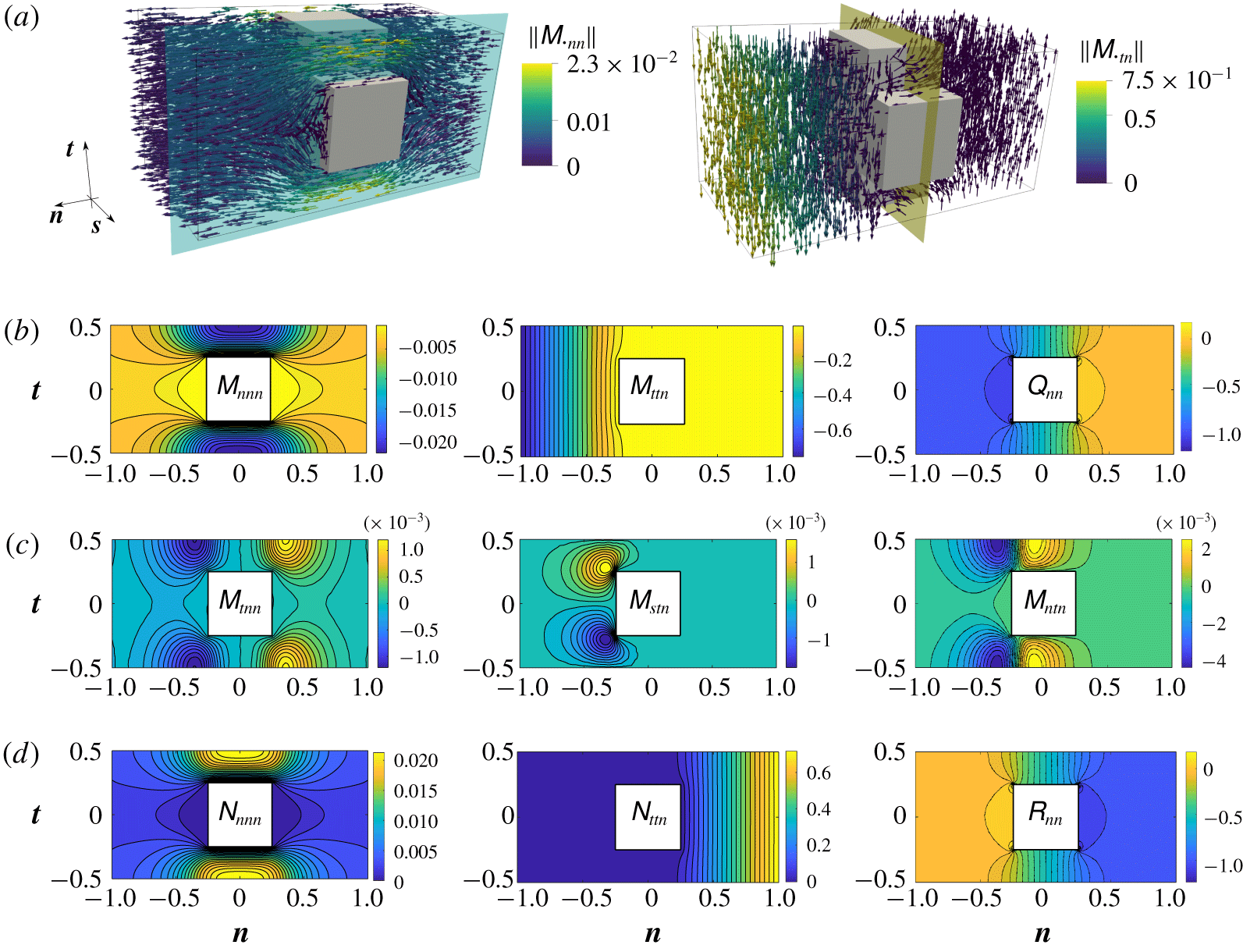
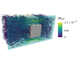
 $\unicode[STIX]{x1D614}_{\cdot tn}$ is given in figure 3(a) for the case of the ordered lattice of cubic pores represented in figure 1. The two frames in figure 3(a) represent respectively the microscopic normal and tangential filtrations of the fluid through the permeable membrane. We note that
 $\unicode[STIX]{x1D614}_{\cdot tn}$ changes direction beyond the pores since a recirculation bubble is created within them. In figures 3(b) and 3(c) some components of the tensors
 $\unicode[STIX]{x1D648}$ and
 $\unicode[STIX]{x1D64C}$ are represented on the plane highlighted in light blue in (a). Since the pore geometry has cubic symmetries, most of the components are antisymmetric (figure 3c) with respect to one of the principal planes. The components of
 $\unicode[STIX]{x1D648}$ along
 $\boldsymbol{s}$ have been missed in the figure since they can be obtained as a
 $90^{\circ }$ rotation on the plane
 $(\boldsymbol{t},\boldsymbol{s})$ of the components along
 $\boldsymbol{t}$. Upon calculating
 $\unicode[STIX]{x1D649}$, it can be seen that it is the opposite to the reflection of the tensor
 $\unicode[STIX]{x1D648}$, with respect to the yellow plane in figure 3(a), while
 $\unicode[STIX]{x1D64D}$ is the reflection of
 $\unicode[STIX]{x1D64C}$ with respect to the same plane.
Solution of the microscopic problems. (a) Vectorial representation of  $\unicode[STIX]{x1D614}_{\cdot nn}$ and
 $\unicode[STIX]{x1D614}_{\cdot tn}$. The vectors, not to scale in order to offer an enhanced view of the microscopic behaviour, are coloured with their magnitude. (b,c) Isocontours of the components of
 $\unicode[STIX]{x1D648}$ and
 $\unicode[STIX]{x1D64C}$ sampled over the light-blue plane of (a). The components in (c) do not contribute to the macroscopic condition (2.6) since their average on the yellow plane of (a) is equal to zero. (d) Entries of the solution of problem (3.14) which contribute to condition (2.6).

We are interested in the averaged values of the microscopic tensors which play a role in the effective condition (2.6). As explained in § 3.4, we use definition (3.15) to deduce the macroscopic counterpart of the microscopic tensors, i.e. we integrate over the yellow plane represented in figure 3(a), getting rid of the fast variable  $\boldsymbol{x}$. The off-diagonal entries of the tensors
 $\bar{\unicode[STIX]{x1D648}}$ and
 $\bar{\unicode[STIX]{x1D649}}$ are zero, owing to the antisymmetries previously reported. The cubic symmetry of the pores implies that
 $\bar{\unicode[STIX]{x1D614}}_{ssn}=\bar{\unicode[STIX]{x1D614}}_{ttn}$, while
 $\bar{\unicode[STIX]{x1D614}}_{nnn}$ is different since the microscopic problems are not periodic along
 $\boldsymbol{n}$. Finally,
 $\bar{\unicode[STIX]{x1D618}}_{nn}$ is different from zero. Due to the symmetric structure of the microscopic cell and boundary conditions we obtain that
 $\bar{\unicode[STIX]{x1D649}}=-\bar{\unicode[STIX]{x1D648}}$ and that
 $\bar{\unicode[STIX]{x1D64D}}=\bar{\unicode[STIX]{x1D64C}}$. The results shown in figure 3 are computed for a cell of normal size equal to
 $l_{n}=4l$. Since the theory does not give information about the choice of
 $l_{n}$, the values of the averaged tensors have to be
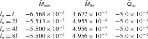
 $l_{n}$-independent, otherwise the macroscopic model would not have a unique solution. This property has been verified numerically and the results are shown in table 1, concluding that
 $l_{n}=4l$ is enough to converge with a tolerance less than
 $0.1\,\%$. The same minimal value of
 $l_{n}$ has been found by Alinovi, Gribaudo & Bottaro (Reference Alinovi, Gribaudo and Bottaro2018) when solving similar microscopic problems associated with the effective slip lengths to be used in the Navier slip condition.
Non-zero numerical values of  $\bar{\unicode[STIX]{x1D648}}$ and
 $\bar{\unicode[STIX]{x1D64C}}$ on increasing the size of the microscopic elementary cell along
 $\boldsymbol{n}$.
 $l_{n}=4l$ is sufficient to reach converged values.

We offered a global overview of the microscopic solution for a given geometry with fixed porosity  $\unicode[STIX]{x1D717}$, defined as
 $$\begin{eqnarray}\unicode[STIX]{x1D717}:=\bar{1},\end{eqnarray}$$
with  $\bar{\cdot }$ the average introduced in (3.15); it measures the fluid ratio on the yellow plane represented in figure 3(a). From the previous description it is still not clear how the tensors are able to measure variations in the microscopic geometry of the pores to be transferred to the equivalent condition (2.6). In order to provide insights in this direction, two parametric studies, varying the geometry of the inclusions, have been performed. We only focus on
 $\unicode[STIX]{x1D648}$ and
 $\unicode[STIX]{x1D64C}$ since the values of
 $\unicode[STIX]{x1D649}$ and
 $\unicode[STIX]{x1D64D}$ can be deduced using the relations described above. The geometries considered are assumed invariant along
 $\boldsymbol{s}$. In this way we deal with two-dimensional microscopic problems whose results can be presented in a more concise and intuitive way.
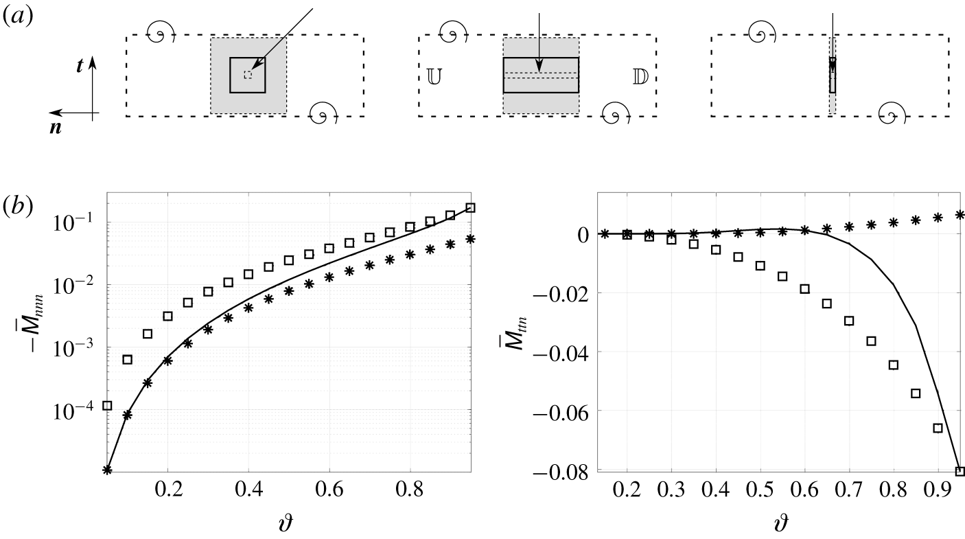
The first parametric study is described in figure 4. Three different geometries for the solid inclusions have been considered in this case (square inclusions and rectangular inclusions elongated in  $\boldsymbol{n}$ or
 $\boldsymbol{t}$), and for each of them the porosity
 $\unicode[STIX]{x1D717}$ ranges from
 $0.05$ to
 $0.95$, as described in figure 4(a). Here,
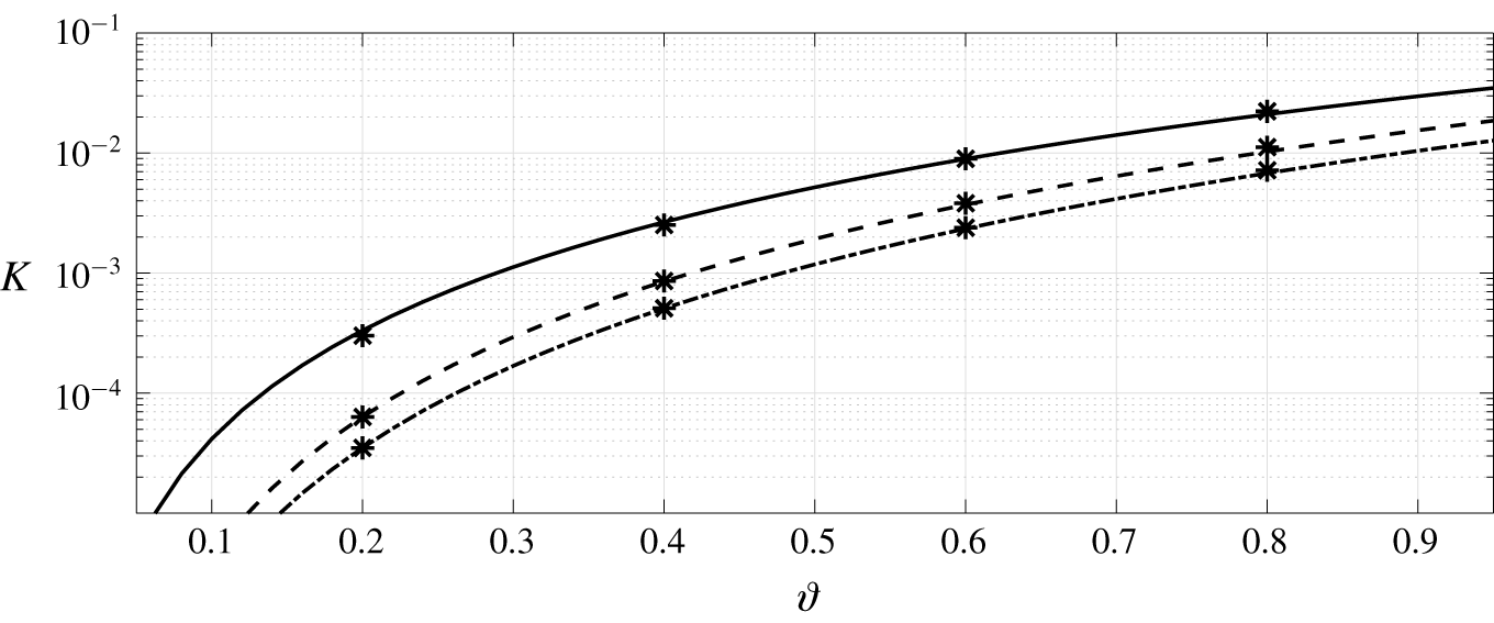
 $\bar{\unicode[STIX]{x1D614}}_{nnn}$, whose intensity is the main factor responsible for the normal fluid filtration, is represented in figure 4(b) for varying
 $\unicode[STIX]{x1D717}$. Analysing its values, if filtration must be enhanced, the third configuration of (a) has to be chosen. An interesting property of
 $\bar{\unicode[STIX]{x1D614}}_{ttn}$ is shown in the right frame of figure 4(b). For the square geometry, a critical value of
 $\unicode[STIX]{x1D717}\approx 0.635$ exists, corresponding to a sign change of
 $\bar{\unicode[STIX]{x1D614}}_{ttn}$. From a macroscopic point of view this sign change corresponds to a flow inversion along
 $\boldsymbol{t}$ across the membrane. This is an indication of the fact that the macroscopic flow can be substantially influenced by the microscopic geometry. Finally, for each case considered,
 $\bar{\unicode[STIX]{x1D618}}_{nn}=\unicode[STIX]{x1D717}/2$.
Non-zero averaged entries of the upward Navier tensor  $\bar{\unicode[STIX]{x1D648}}$ for the three different types of membrane inclusions represented in (a). The solid lines represent the values of
 $\bar{\unicode[STIX]{x1D648}}$ in the case of square solid inclusions (top left image), the stars refer to the components of
 $\bar{\unicode[STIX]{x1D648}}$ for the top central case, where the normal size of the inclusion is kept equal to the side of the square inclusion which realizes
 $\unicode[STIX]{x1D717}=0.95$, and the squares refer to the top right case where the normal size of the inclusions is equal to that of the square inclusion for
 $\unicode[STIX]{x1D717}=0.05$. The arrows in (a) indicate how the inclusions have been modified to decrease
 $\unicode[STIX]{x1D717}$. For each case the solid grey rectangle corresponds to
 $\unicode[STIX]{x1D717}=0.5$ while the dashed ones are referred to
 $\unicode[STIX]{x1D717}=0.05,0.95$.

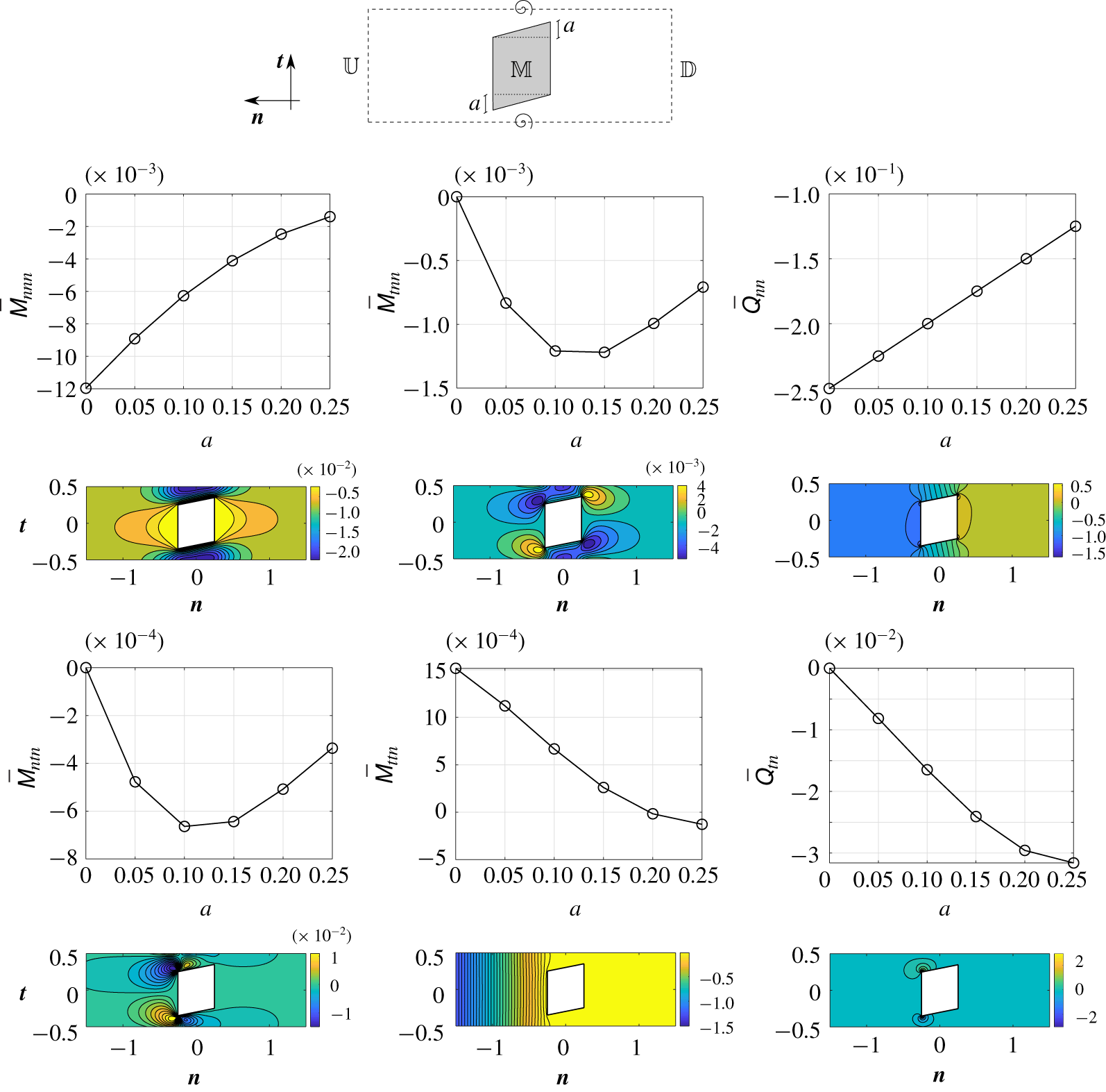
Anisotropy evaluation for  $\bar{\unicode[STIX]{x1D648}}$ and
 $\bar{\unicode[STIX]{x1D64C}}$ in the case of parallelogram shaped inclusions. The parameter
 $a$ ranges from
 $0$ to
 $0.25$. Under each graph, the isocontours of the corresponding component are shown for the case
 $a=0.1$.

The geometries previously considered are isotropic and no tangential fluid velocities can be generated if the flow is normal to the centreline  $\mathbb{C}$ of the membrane. A second parametric study is carried out to include the effects of anisotropy on the averaged tensors. The geometry sketched in figure 5 has been considered and modified to exhibit an increasing level of anisotropy, by varying the parameter
 $a$. The microscopic geometries analysed in this section are very few, but they clearly show the flexibility of the method utilized, and its ability to catch the averaged effects of microscopic anisotropy is clear. Clearly, the price to pay for having a pure tangential effect on the flow field (
 $\bar{\unicode[STIX]{x1D614}}_{ttn}$) is to decrease the pure normal filtration (
 $\bar{\unicode[STIX]{x1D614}}_{nnn}$). Finally, if we mirror the geometry along
 $\boldsymbol{t}$, the same values of normal filtration are recovered, but the tangential filtration has the opposite sign, being able to reverse the tangential macroscopic flow (this will be verified later on in the macroscopic test cases). As a consequence, having in mind how the microscopic averaged quantities influence the macroscopic flow, with this approach we can potentially design the microscopic geometry in order to guide the macroscopic flow in the desired way. Since in the literature such a formal framework to microscopically analyse flows across thin membranes is not present, the best way to validate the microscopic results is to understand if they are able to reproduce well the macroscopic flow field once the equivalent model is utilized. Nevertheless, in appendix A, we provide a further physical interpretation and validation of the tensor
 $\bar{\unicode[STIX]{x1D648}}$ in the particular case of membranes with cylindrical pores.
4.2 Representative test cases for the effective jump model
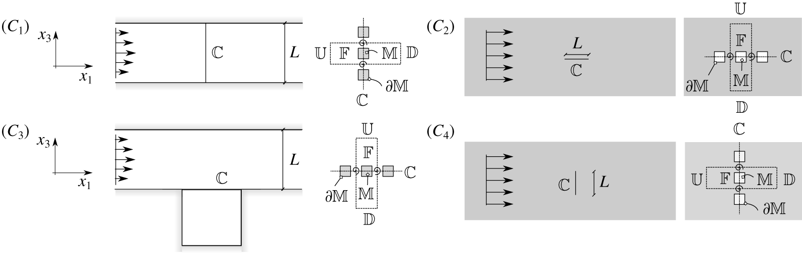
We validate model (2.6) for each test case sketched in figure 6. In all cases, the map, from the local curvilinear frame of reference, used to express the microscopic tensors in the absolute Cartesian frame, is trivial, while a more complex surface with space-dependent tangent and normal directions is presented in § 4.4. All configurations show substantial differences. These differences are quantified thanks to the normalizations adopted in the upward and downward regions. In configuration  $C_{1}$ the fluid is compelled to pass through the membrane, which ideally splits the fluid domain into two portions; to preserve flow rate, the representative fluid velocity within the pores is the same as in the rest of the domain. In configurations
 $C_{2}$,
 $C_{3}$ and
 $C_{4}$ the fluid is not constrained to pass through the pores and the reference velocity within the membrane is, in principle,
 $\unicode[STIX]{x1D716}$ times smaller than in the outer region. In configuration
 $C_{2}$ the flow field is symmetric with respect to the line
 $x_{3}=0$ which passes over
 $\mathbb{C}$ and the upward and downward scales are the same. From a macroscopic point of view this implies that both the up- and downward contributions have to be considered in (2.6). In configurations
 $C_{3}$ and
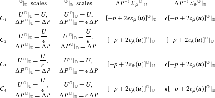
 $C_{4}$ the fluid flow in the downward region has representative velocities and pressure differences which are negligible if compared to those in the upward region. Table 2 shows the pressure and velocity scales for each configuration, together with the normalized stress tensor in the upward and downward regions. Summarizing, if we approximate the flow field at the leading order, the contribution given by the downward Navier tensor
 $\bar{\unicode[STIX]{x1D649}}$ in (2.6) has to be neglected in configurations
 $C_{1}$,
 $C_{3}$ and
 $C_{4}$. Moreover, in the case of configuration
 $C_{1}$, also the viscous part of the upward stress tensor is negligible.
Test cases selected to describe the possible situations of fluid flows across membranes. In all cases invariance along  $x_{2}$ is assumed. Configuration
 $(C_{1})$: channel split by a vertical membrane positioned in
 $\mathbb{C}$. The fluid flows from left to right. Configuration
 $(C_{2})$: uniform constant flow in an unbounded domain encountering a membrane, positioned in
 $\mathbb{C}$, parallel to its direction. Configuration
 $(C_{3})$: channel with a cavity on the bottom wall. A membrane divides the cavity from the rest of the fluid domain. Configuration
 $(C_{4})$: the flow configuration is the same as in
 $(C_{2})$ but the membrane is orthogonal to the flow direction.

Outer scales in the downward and upward regions and non-dimensional outer stresses for the 4 configurations sketched in figure 6. The parameter  $\unicode[STIX]{x1D750}$ in bold highlights which contributions must be neglected in the leading-order approximation (2.6) of the velocity in
 $\mathbb{C}$.

From top, isocontours of horizontal velocity  $u_{1}$, vertical velocity
 $u_{3}$ and pressure
 $p$ for configuration
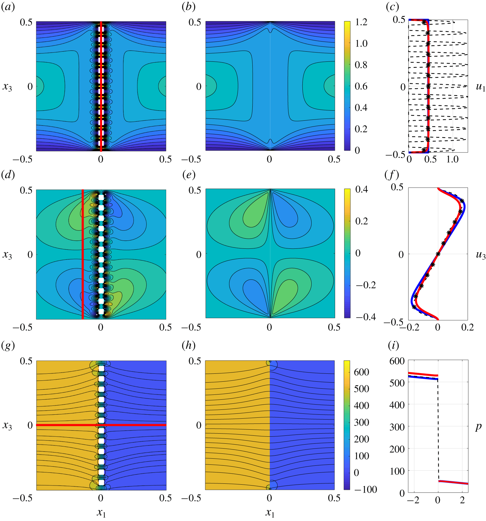
 $C_{1}$, computed using the full Stokes equations (a,d,g) or the equivalent model (2.6), (b,e,h). In both cases we impose a parabolic velocity profile at the inlet (
 $x_{1}=-5$) and we set a constant pressure at the outlet (
 $x_{1}=5$). In (g,h), the black solid lines are the flow streamlines. Panels (c,i,f) represent the horizontal velocity and pressure sampled on
 $\mathbb{C}$, and the vertical velocity sampled on the line
 $x_{1}=-0.1$. Dashed black profiles refer to the solution of the full Stokes equations and solid red lines to the solution of model (4.3). The stars represent the averaged profile of the full-scale solution extracted using definition (3.15). The solid blue lines represent the solution computed using the model developed in Bourgeat et al. (Reference Bourgeat, Gipouloux and Marusic-Paloka2001).

We now systematically compare each configuration with direct numerical simulations of the fluid flow across thin membranes. All results shown in this section are rendered non-dimensional by normalizing lengths with  $L$, velocities with
 $U^{\,\mathbb{O}}|_{U}$ and pressure with
 $\unicode[STIX]{x1D70C}{U^{\,\mathbb{O}}|_{U}}^{2}$. With these normalizations equation (2.6) becomes
 $$\begin{eqnarray}\left.\begin{array}{@{}c@{}}u_{i}|_{\mathbb{C}}=\unicode[STIX]{x1D716}[\bar{\unicode[STIX]{x1D614}}_{ijk}\unicode[STIX]{x1D6F4}_{jk}|_{\mathbb{C}^{-}}+\bar{\unicode[STIX]{x1D615}}_{ijk}\unicode[STIX]{x1D6F4}_{jk}|_{\mathbb{C}^{+}}],\\ u_{i}|_{\mathbb{C}}=u_{i}|_{\mathbb{C}^{-}}=u_{i}|_{\mathbb{C}^{+}}.\end{array}\right\}\end{eqnarray}$$
For all cases the microscopic structure of the membrane corresponds to the square configuration introduced in figure 4 and the porosity  $\unicode[STIX]{x1D717}$ is set to 0.5.
4.2.1 Configuration  $C_{1}$

We focus our attention on configuration  $C_{1}$. In this case, using the normalizations described in table 2, and observing that
 $(\boldsymbol{t},\boldsymbol{n})=(\boldsymbol{e}_{1},\boldsymbol{e}_{3})$, we obtain that only the pressure contribution of the upward stress tensor must be considered, i.e.
 $$\begin{eqnarray}\displaystyle & \displaystyle u_{1}|_{\mathbb{C}}=-\unicode[STIX]{x1D716}\bar{\unicode[STIX]{x1D614}}_{111}p|_{\mathbb{C}^{-}}, & \displaystyle\end{eqnarray}$$
 $$\begin{eqnarray}\displaystyle & \displaystyle u_{3}|_{\mathbb{C}}=-\unicode[STIX]{x1D716}\bar{\unicode[STIX]{x1D614}}_{311}p|_{\mathbb{C}^{-}}. & \displaystyle\end{eqnarray}$$
For this test case, the parameter  $\unicode[STIX]{x1D716}$ has been chosen equal to 0.08 to push the validation of the model to non-infinitesimal values of
 $\unicode[STIX]{x1D716}$. Different values of
 $\unicode[STIX]{x1D716}$ have been chosen for other configurations and they are listed in the captions of the corresponding figures. Since for isotropic inclusions
 $\bar{\unicode[STIX]{x1D614}}_{311}=0$, we obtain that the vertical velocity
 $u_{3}|_{\mathbb{C}}$ is equal to zero. The flow field is represented via the isocontours of velocities and pressure in figure 7. On the left, the solution of the full-scale problem is represented while on the right the equivalent macroscopic fields are sketched. Pointwise and macroscopic fields are qualitatively similar in the region around the membrane; they show only small-scale differences near the pores. It is, however, clear that the model well describes the fluid behaviour in an average sense; as can be evinced from the isocontours of figure 7, the small-scale flow structures generated by the presence of the solid inclusions cannot be reproduced. On the contrary, the macroscopic effects of these inclusions on the flow are perfectly simulated. To assess the validity of the model and quantify its appropriateness, we compare the solutions on
 $\mathbb{C}$. In the right column of figure 7 the dashed profiles correspond to the pointwise solution of the Stokes equations, solved at the pore scale, while the solid red lines represent the macroscopic solution computed using (4.4) and (4.5). We observe that the red line perfectly matches the stars, deduced from the dashed profile applying average (3.15). The strong pressure jump generated across the membrane is correctly estimated by the macroscopic model with an error of approximately
 $4\,\%$. Maximum discrepancies between the macroscopic and the full-scale velocities are less than
 $2\,\%$ in the internal region of the membrane. This value, fully within the theoretical prediction (
 $O(\unicode[STIX]{x1D716})\approx 8\,\%$), increases when approaching the solid walls of the channel, where the periodicity assumption along the tangent to the surface direction within the microscopic elementary cell becomes inaccurate. Highest discrepancies can be noticed near the walls of the channel where the homogenization assumption is violated (i.e. technically speaking, the periodicity along the tangential directions is no longer valid). This can be seen, in particular, in the graphs representing the vertical velocity
 $u_{3}$. For this particular flow configuration, the model developed in Bourgeat et al. (Reference Bourgeat, Gipouloux and Marusic-Paloka2001) can be used to find the solution, represented by the solid blue line in the right frames of figure 7. This model consists in matching the solution of an outer, macroscopic, problem, with the solution of an inner boundary layer problem which takes the microscopic structure of the membrane into account. As can be evinced by the figure, while the pressure jump is well estimated by the model in Bourgeat et al. (Reference Bourgeat, Gipouloux and Marusic-Paloka2001), the approximation of the velocity is degraded, especially approaching the boundaries of the filter since the model allows only constant velocity profiles across the membrane.
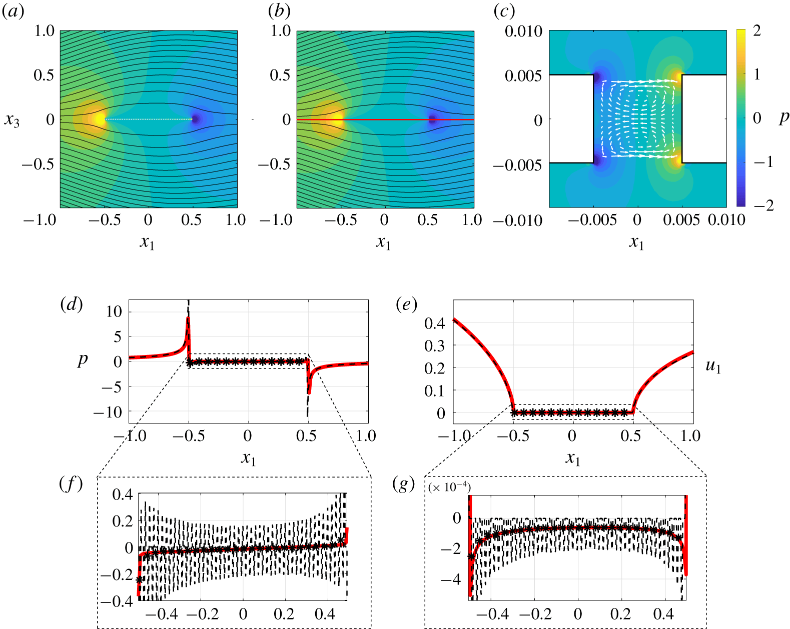
Fluid flow analysis of configuration  $C_{2}$. (a–c) Isocontours of pressure are represented for the full-scale simulation (a) and the macroscopic model (b), together with the flow streamlines in black. Panel (c) shows a zoom in on the microstructured membrane and the white arrows represent the velocity field. (d,e) Sampling of pressure (left) and horizontal velocity on the red line sketched in (b). Dashed black profiles refer to the solution of full Stokes equations and solid red lines to the solution of model (4.3). The stars represent the averaged profile of the full-scale solution extracted using definition (3.15). In (f,g) zooms of
 $p$ and
 $u_{1}$ on the membrane are shown. The parameter
 $\unicode[STIX]{x1D716}$ is equal to 0.02.

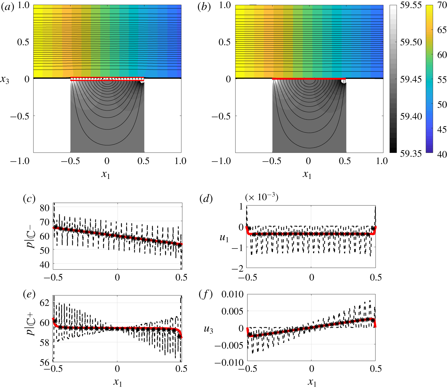
Fluid flow analysis of configuration  $C_{3}$. (a,b) Isocontours of pressure are represented for the full-scale simulation (a) and the macroscopic model (b), together with the flow streamlines in black. (c,e) Pressure sampled on the upward (c) and downward sides (e), at the positions highlighted in red in (a). (d,f) Horizontal (d) and vertical (f) velocity sampled on
 $\mathbb{C}$. Dashed black profiles refer to the solution of the full Stokes equations and solid red lines to the solution of model (4.3). The stars represent the averaged profile of the full-scale solution extracted using definition (3.15). The parameter
 $\unicode[STIX]{x1D716}$ is equal to 0.04.

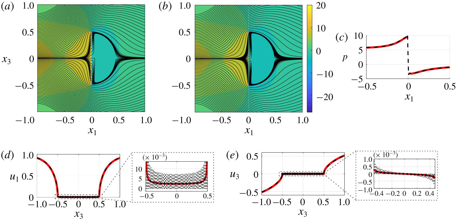
Fluid flow analysis of configuration  $C_{4}$. (a,b) Isocontours of pressure are represented for the full-scale simulation (a) and the macroscopic model (b), together with the flow streamlines in black. Panel (c) shows the pressure sampled on the line
 $x_{3}=0$. (d,e) The horizontal and vertical velocities, with the corresponding zoom on
 $\mathbb{C}$ are sampled on the line
 $x_{1}=0$. Dashed black profiles refer to the solution of the full Stokes equations and solid red lines to the solution of model (4.3). The stars represent the averaged profile of the full-scale solution extracted using definition (3.15). The parameter
 $\unicode[STIX]{x1D716}$ is equal to 0.02.

4.2.2 Configuration $C_{2}$

As already mentioned, in configuration  $C_{1}$, the order of magnitude of the inner velocity is the same as the outer, while in the remaining configurations the ratio between inner and outer velocities is of order
 $\unicode[STIX]{x1D716}$. This is the case of configuration
 $C_{2}$ whose pressure and horizontal velocity are shown in figure 8 over the line
 $x_{3}=0$, with the corresponding zoom over
 $\mathbb{C}$. Figure 8(a,b) shows that, macroscopically, the effective and full-scale flow fields are identical, but, microscopically, the equivalent model cannot reproduce the complexity of the flow field, sketched in panel (c) by means of the velocity field (white arrows) and isocontours of pressure. In this configuration, since the fluid flow has equal representative scales in the downward and upward region, the complete equivalent condition has been used.
4.2.3 Configuration $C_{3}$

Conversely to the previous case, in configuration  $C_{3}$, whose associated profiles can be observed in figure 9 over
 $\mathbb{C}$, the downward scales are negligible with respect to the upward. This can be observed for instance in terms of the pressure, evaluated in the upward region (panel c) and in the downward region (panel e). The two pressure profiles, perfectly reproduced by the equivalent field, show that the pressure gradient in the downward region is much smaller than the one in the upward.
4.2.4 Configuration $C_{4}$

Finally, in case  $C_{4}$ (shown in figure 10), whose alignment between the flow direction and the membrane direction is the same as configuration
 $C_{1}$, we observe that the fluid behaves in a way completely different if it is not compelled to pass across the membrane. Also, a vertical velocity is generated in this case, which, even small, is perfectly evaluated by the equivalent model. The four configurations presented cover many possible combinations of the inner and outer scales and constitute a solid validation of condition (2.6). In the next paragraphs we investigate some useful functionality of the new model.
4.3 Large-scale effects of small-scale anisotropy
Model (2.6) has no restrictions regarding the microscopic geometry of the membrane’s pores. Modifications in the microscopic topology have non-negligible consequences for the macroscopic flow (i.e. on the values of  $\bar{\unicode[STIX]{x1D648}}$,
 $\bar{\unicode[STIX]{x1D649}}$,
 $\bar{\unicode[STIX]{x1D64C}}$ and
 $\bar{\unicode[STIX]{x1D64D}}$). Microscopic problem (3.13) allows us to precisely quantify these geometrical modifications. Our purpose here is to show that the changes evaluated at the microscale have coherent effects on the macroscale. We replace in configuration
 $C_{1}$ a membrane with the anisotropic microstructure analysed in figure 5. A second configuration is obtained by mirroring this geometry with respect to
 $\mathbb{C}$. As already observed in § 4.1, owing to anisotropy,
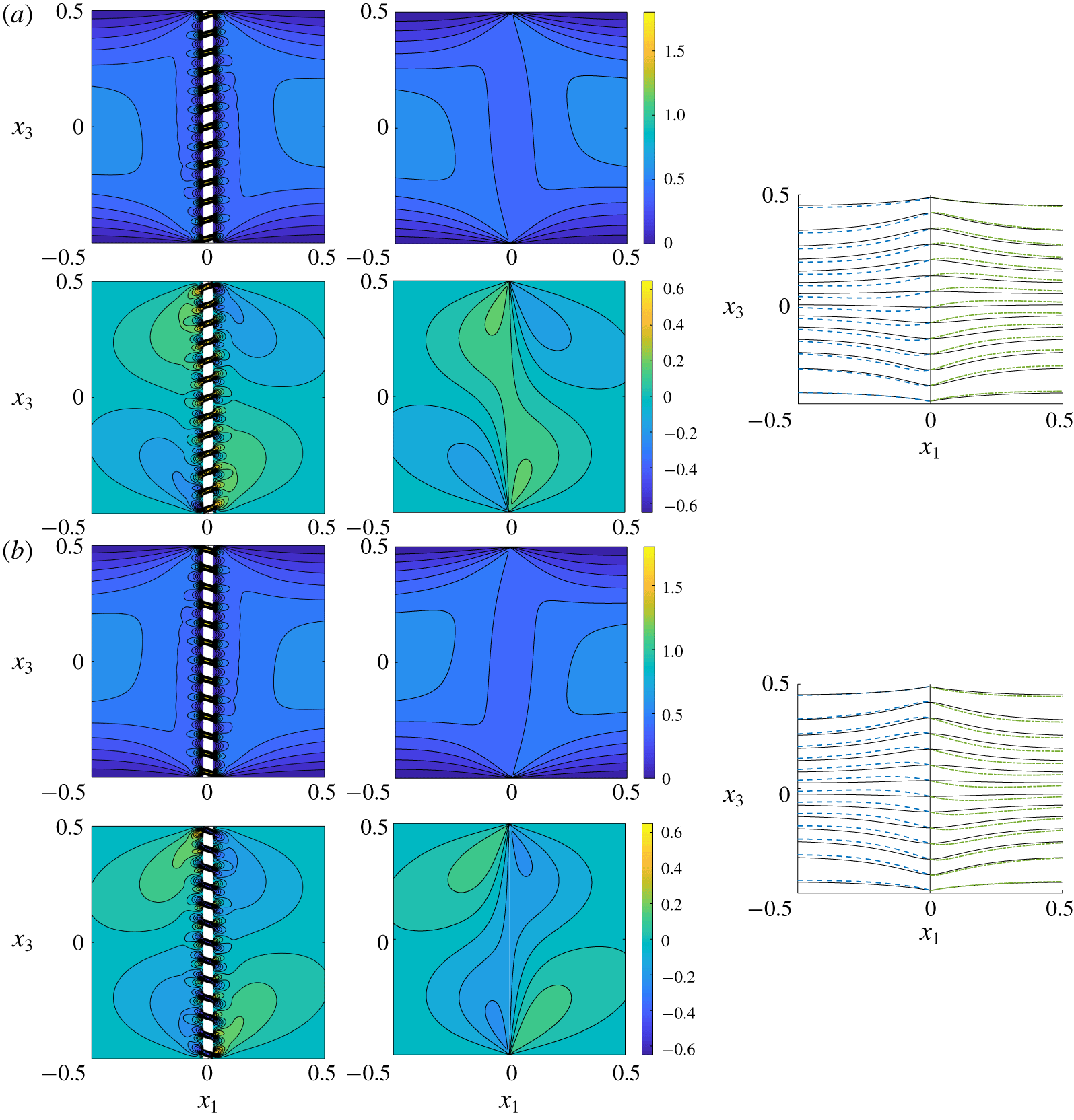
 $\bar{\unicode[STIX]{x1D614}}_{ttn}=\bar{\unicode[STIX]{x1D614}}_{311}$ is different from zero. This implies that the vertical velocity across the membrane is different from zero. Figure 11 shows the entire fields in a region across the membrane (direct numerical simulations of the Stokes equations on the left and macroscopic solution on the right). As in the
 $C_{1}$ configuration analysed in the previous section, even if
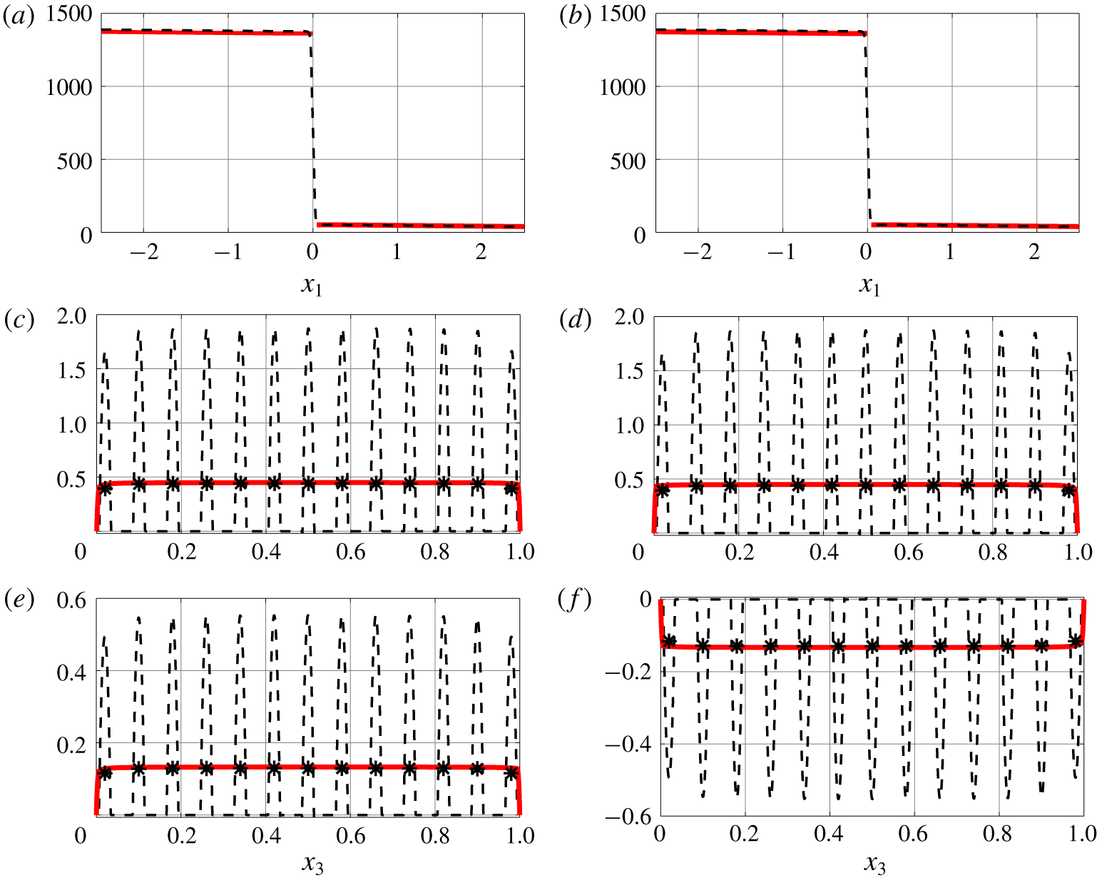
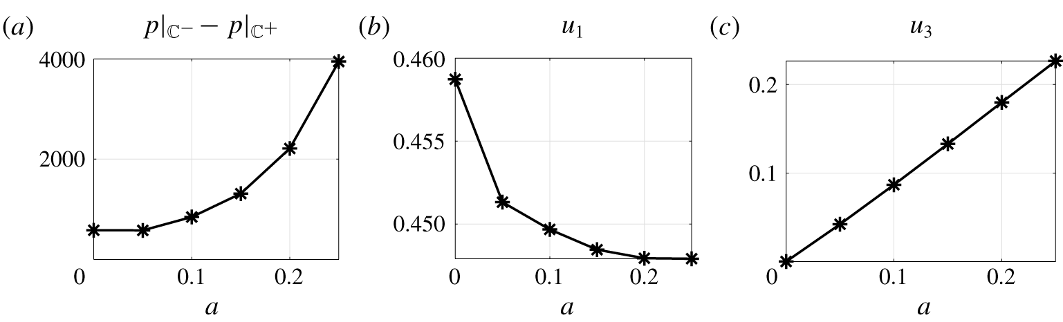
 $\unicode[STIX]{x1D716}$ is 0.08, the macroscopic fields are identical up to differences confined to the region where the small scale is dominant. Focussing on the membrane, quantitative comparisons between the macroscopic model and the full solution, for pressure and velocity profiles, are represented in figure 12, showing a perfect agreement. Mirroring the microscopic geometry, the only difference noticed with the previous case is an inversion of the vertical velocity (cf. panels (e,f) of figure 13). Finally, the parametric study carried out in § 4.1 to investigate the behaviour of the microscopic tensors when the anisotropy of the pores is increased, is reproduced macroscopically, and some fundamental quantities are shown in figure 13 for varying values of the parameter
 $a$. From left, the pressure jump
 $p|_{\mathbb{C}^{-}}-p|_{\mathbb{C}^{+}}$ and horizontal and vertical velocities
 $u_{1}|_{\mathbb{C}}$ and
 $u_{3}|_{\mathbb{C}}$, all evaluated in the origin of the axes, are shown. These values are significant since the profiles are almost constant with respect to
 $x_{3}$ and, as evinced by the figure, they can be controlled by only varying the microscopic geometry (or, equivalently, the values of the microscopic tensors). With the few results presented in this section it is clear that the effects on the macroscopic flow of the microscopic geometry are perfectly captured by the model, which is, consequently, a new tool to drive the design of thin membranes to obtain the desired flow behaviour.
Velocity fields and streamlines in configuration  $C_{1}$ when the membrane has microscopic anisotropic structure. (a) The structure of the pores corresponds to that described in figure 5 for
 $a=0.15$. (b) The pores are realized by mirroring with respect to
 $\mathbb{C}$ the geometry of (a). For both (a) and (b) the top and bottom rows represent the horizontal and vertical velocities evaluated solving the full Navier–Stokes equations (left column) or the equivalent model (2.6). On the right column the streamlines are represented for the two cases: the dashed blue lines refer to the fields in the upward region while the green dashed-dotted lines refer to those in the downward region. The black lines refer to the isotropic case whose velocity fields are represented in figure 7.

Pressure and velocity fields of the configurations introduced in figure 11(a) (a,c,e) and figure 11(b) (b,d,f). The pressure (a,b) has been evaluated along the centreline of the channel, while the horizontal and vertical velocities (c,d and e,f respectively) have been evaluated along  $\mathbb{C}$. Dashed black profiles refer to the solution of the full Stokes equations and the solid red line to the solution of model (2.6). The stars represent the average profile of the full solution extracted using definition (3.15).

Some macroscopic quantities have been evaluated in configuration  $C_{1}$ when the membrane has the microscopic structure described in figure 5. From left, pressure jump across the membrane
 $p|_{\mathbb{C}^{-}}-p|_{\mathbb{C}^{+}}$, horizontal and vertical velocity along the centreline of the channel,
 $u_{1}|_{\mathbb{C}}$ and
 $u_{3}|_{\mathbb{C}}$.

4.4 Generically shaped surfaces
In this section we complete our work showing that, with the tensorial approach used, we are able to apply the condition to generically shaped perforated surfaces. In the configurations previously analysed, the shape of the membrane is such that the local frame of reference  $(\boldsymbol{s},\boldsymbol{t},\boldsymbol{n})$ had constant orientation with respect to the absolute Cartesian frame of reference. In the case of more complex membrane shapes, the maps between the two frames of reference have to be explicitly specified. As a result, we deal with tensors which are not diagonal and every component of the stress tensor contributes to define the velocity in
 $\mathbb{C}$. We apply the model in case of a cylindrical permeable shell immersed in a uniform constant flow. The shell is realized by rotating the square pore geometry of figure 5 and is such that
 $\unicode[STIX]{x1D700}=0.02$ and
 $\unicode[STIX]{x1D717}=0.5$. The flow configuration has been chosen such that the characteristic scales are the same as in case
 $C_{3}$ of § 4.2 and, hence, only the upward stress contributes in (2.6). To successfully apply the equivalent condition we need to specify the upward Navier tensor
 $\bar{\unicode[STIX]{x1D648}}$ in Cartesian coordinates
 $$\begin{eqnarray}\unicode[STIX]{x1D614}_{ijk}=\bar{\unicode[STIX]{x1D614}}_{ttn}\boldsymbol{t}\wedge \boldsymbol{t}\wedge \boldsymbol{n}+\bar{\unicode[STIX]{x1D614}}_{tnn}\boldsymbol{t}\wedge \boldsymbol{n}\wedge \boldsymbol{n}+\bar{\unicode[STIX]{x1D614}}_{ntn}\boldsymbol{n}\wedge \boldsymbol{t}\wedge \boldsymbol{n}+\bar{\unicode[STIX]{x1D614}}_{nnn}\boldsymbol{n}\wedge \boldsymbol{n}\wedge \boldsymbol{n},\end{eqnarray}$$
where  $\boldsymbol{t}=(0,-\sin (\unicode[STIX]{x1D6FC}),\cos (\unicode[STIX]{x1D6FC}))$,
 $\boldsymbol{n}=(0,\cos (\unicode[STIX]{x1D6FC}),\sin (\unicode[STIX]{x1D6FC}))$ and
 $\unicode[STIX]{x1D6FC}=\tan ^{-1}(x_{3}/x_{1})$ while
 $\wedge$ denotes the outer product
 $a_{i}\wedge b_{j}:=a_{i}b_{j}$. In this way
 $\bar{\unicode[STIX]{x1D648}}$ is a full tensor which depends on
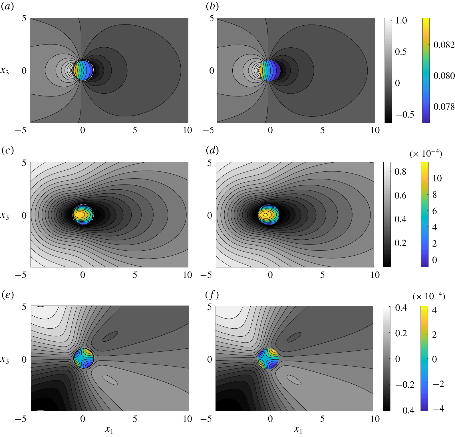
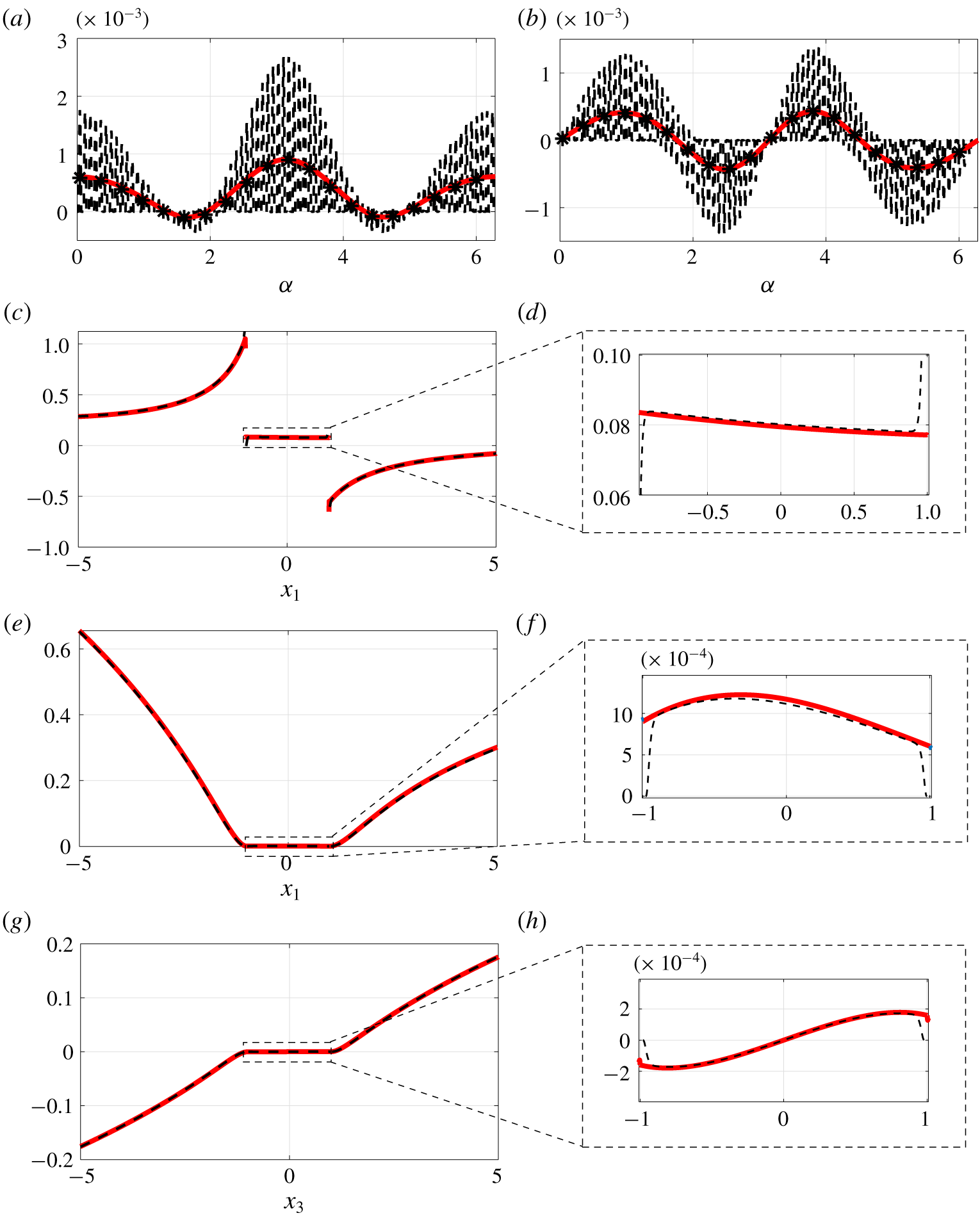
 $(x_{1},x_{3})$. Figure 14 shows the velocity and pressure fields (full-scale solution of the Stokes equations on the left) in the region around the permeable shell. The flows in the upward and downward regions look similar, but it is hard to quantify the exactitude of the model without looking at local quantities, which are shown in figure 15. The macroscopic horizontal and vertical velocities on
 $\mathbb{C}$ match the averaged ones with an error smaller than
 $\unicode[STIX]{x1D716}$. In (c–f) the pressure and velocities have been evaluated over the line
 $x_{3}=0$ and a zoom in on the region inside the shell is provided, showing that the macroscopic fields perfectly match the Stokes solution despite the fact that, in the latter, the horizontal velocity goes to zero since the no-slip condition is enforced on the surface of the solid inclusions. The same holds for the vertical velocity, represented in (g,h) on the line
 $x_{1}=0$. This last case shows that the model developed is a flexible tool able to reproduce the feedback on the flow of generically shaped thin perforated surfaces.
From top: isocontours of the pressure, horizontal and vertical velocity for the case of uniform flow past a permeable cylindrical shell, found by solving the full Stokes equations (a,c,e) or the macroscopic model (2.6) (b,d,f).

Velocities and pressure sampled at different positions in the case of uniform flow past a permeable cylindrical shell. Panels (a,b), horizontal and vertical velocities evaluated on  $\mathbb{C}$, angle
 $\unicode[STIX]{x1D6FC}$ is evaluated counterclockwise starting from the rear stagnation point. Panels (c–f), pressure and horizontal velocity on a horizontal line passing through the centre of the cylinder and zoom in on the region within the cylinder. Panels (g,h), vertical velocity on a vertical line passing through the centre of the cylinder with a zoom in on the region within the cylinder. Dashed lines represent the solution of the Stokes equations, while the red solid lines are deduced by the solution of the macroscopic model (2.6). The stars represent the average extrapolated from solution of the Stokes equations using definition (3.15).

5 Conclusions and outlook
In the present work we have developed an equivalent model to simulate the effects of thin porous surfaces (called here membranes) on a surrounding fluid flow. The model, summarized in system (2.6), is purely macroscopic, i.e. it allows us to simulate the perforated microstructured surface like a constraint on the flow imposed on a smooth surface. This smooth surface is an infinitely thin region where the fluid changes its effective properties and behaves differently than in the rest of the domain. The velocity in this region is described by a linear combination of the upward and downward stress tensors. The coefficients of the linear combination are the averaged entries of tensors which can be calculated by solving Stokes problems on a microscopic domain enforced by boundary conditions which physically represent the macroscopic feedback on the microscopic domain and vice versa. These conditions are formally deduced by matching the outer macroscopic flow with the inner multiscale flow. The model, which allows us to evaluate the effects of the microstructured surface on the macroscopic flow, lists, among its strengths, generality regarding (i) the microscopic topology of the membrane (only periodicity along the tangential to the surface direction is assumed) and (ii) the macroscopic shape of the membrane (whose only constraint is  $l/R\approx \unicode[STIX]{x1D716}$ with
 $R$ the radius of curvature of the surface). A third important aspect consists of the fact that, thanks to the formalism used, the condition is applicable to every flow situation, provided that the outer upward and downward scales are estimated, as in table 2. The fact that the inertia of the flow is assumed to be a priori negligible is not restrictive, as shown by Zampogna et al. (Reference Zampogna, Magnaudet and Bottaro2019), and the equivalent equations can be extended to the case of outer inertial flows. In this case, in fact, even if the outer Reynolds number, based on the macroscopic length scale
 $L$ and on an outer reference velocity
 $U^{\,\mathbb{O}}$, is high, the inner Reynolds number, based on the inner velocity scale and on the microscopic length scale
 $l$, can be small, implying that the leading-order equations remains unchanged.
The model developed can be a tool in designing membranes; from a purely mechanical point of view, the selectivity of the membrane is identified by the pore size, while its permeability is measured by the normal component of the Navier tensor  $\bar{\unicode[STIX]{x1D614}}_{nnn}$, as shown in appendix A. Maximizing the permeability by keeping a determined selectivity means, under the framework introduced in the present paper, determining a maximum for
 $\bar{\unicode[STIX]{x1D614}}_{nnn}$ for a given pore size (i.e. porosity). Even if it is clear that this cannot be done in the absolute sense without an inverse formulation of the problem, the cases provided in figure 4 represent a partial solution for a specific geometrical configuration and tell that, for a given fixed selectivity, geometry 3 is preferable to geometry 1 or 2, since the associated Navier tensor, proportional to the fluid velocity at the membrane, is higher.
We also observe that, in some sense, the model is a generalization of Darcy’s law which, under certain flow conditions, can be seen as a subpart of the difference between the upward and downward stresses. To better explain this concept, let us consider case  $C_{1}$ and recall equations (4.4) and (4.5). In dimensional form these equations can be rewritten as
 $$\begin{eqnarray}\hat{u} _{i}|_{\mathbb{C}}=-\frac{l}{\unicode[STIX]{x1D707}}\bar{\unicode[STIX]{x1D614}}_{ijk}\unicode[STIX]{x1D6FF}_{jk}\hat{p}|_{\mathbb{C}^{-}}.\end{eqnarray}$$
Looking at the order  $\unicode[STIX]{x1D716}$ terms which play a role in the boundary conditions of cell problems for the configuration
 $C_{1}$, we can intuitively anticipate that the order
 $\unicode[STIX]{x1D716}$ approximation of the velocity in
 $\mathbb{C}$ can be written, in dimensional variables, as
 $$\begin{eqnarray}\hat{u} _{i}|_{\mathbb{C}}=-\frac{l}{\unicode[STIX]{x1D707}}\bar{\unicode[STIX]{x1D614}}_{ijk}(\hat{p}|_{\mathbb{C}^{-}}-\hat{p}|_{\mathbb{C}^{+}})\unicode[STIX]{x1D6FF}_{jk}+l\bar{\unicode[STIX]{x1D614}}_{ijk}^{\prime }\hat{\unicode[STIX]{x1D716}}_{jk}(\hat{\boldsymbol{u}})|_{\mathbb{C}^{-}}+l\bar{\unicode[STIX]{x1D614}}_{ijk}^{\prime \prime }\hat{\unicode[STIX]{x1D716}}_{jk}(\hat{\boldsymbol{u}})|_{\mathbb{C}^{+}},\end{eqnarray}$$
where  $\unicode[STIX]{x1D648}^{\prime }$ and
 $\unicode[STIX]{x1D648}^{\prime \prime }$ are the solution of some associated microscopic problems. It is clear that neither equation (5.1) nor equation (5.2) are Darcy’s law, which only partially contributes to (5.2). Using Darcy’s law in the present case would mean neglecting all contributions depending on the strain tensor in (5.2), which could be as important as the upward pressure contribution, depending on the macroscopic flow configuration. This example shows how postulating already known models to simulate an arbitrary physics can involve unexpected risks. From this point of view, the permeability tensor makes rigorous sense only when a second-order approximation of the flow is used and the viscous part of the stress tensor is negligible with respect to the pressure part in (5.2). In all other cases, the Navier tensors have to be considered as more general entities. Equation (5.2) shows that the upward Navier tensor
 $\bar{\unicode[STIX]{x1D614}}_{ijk}$, found in the present paper, is a direct measure of the classical permeability tensor which can be easily recovered by experimental measurements. This has been also shown in appendix A, where a comparison with the Sampson–Weissberg formula has been provided.
The present work opens several research paths. First of all, since only the hydrodynamics of flows across thin surfaces has been studied, future works will be developed to study transport of solutes across membranes in order to deduce, via homogenization, effective diffusion coefficients for these devices. This can be done in two instances: if the characteristic size of the pores is much larger than that of the solute particles, a continuum approach can be used to evaluate the effective diffusivity across the membrane (which, in principle, depends only on the pores shape and flow regime). On the contrary, for comparable pore and particle sizes, multiphase homogenization (cf. for instance, Picchi & Battiato (Reference Picchi and Battiato2018)) should be applied to deduce the effective properties of the membrane, which in this case depend also on the particles shape.
Since the structure of membranes can be complex and, in principle, characterized by more than two length scales, extensions of the model will be considered in this direction, based on the idea of sequential homogenization (cf. for instance, Korneev & Battiato (Reference Korneev and Battiato2016)). As mentioned before, we have assumed that, from a microscopic point of view, the permeable surface can be realized as a periodic repetition of a single unitary structure. In view of applications such as flow optimization and control, it is useful to understand under which bounds the microscopic structure can locally vary, to be able to assume microscopic periodicity. As a goal, for instance, to enhance mixing phenomena, it should be possible to locally manipulate the microscopic structure of the porous membrane or, upon a generalization towards inertial regimes, to design innovative devices to control the flow in external aerodynamics applications.
In a near future, we do not exclude the possibility of extending the model developed here, which applies to all those devices where the fluid behaviour is well described by continuum mechanics equations (interesting applied situations can be identified in microfilters for medical purposes, cf. for instance, Liu et al. (Reference Liu, Xu, Dai, Li and Wang2018), in the description of aqueous solutions in sieve tubes, in particular across sieve plates, as in Jensen et al. (Reference Jensen, Berg-Sørensen, Bruus, Holbrook, Liesche, Schulz, Zwieniecki and Bohr2016)), to almost non-continuum, subnanometric, sizes by using pseudo-continuum approaches like the one used in Gravelle et al. (Reference Gravelle, Joly, Detcheverry, Ybert, Cottin-Bizonne and Bocquet2013) to describe fluid flows in carbon nanotubes.
In the present paper we analysed rigid membranes. The model developed can be enriched, modelling the deformability of the membrane, in order to simulate the behaviour of non-stiff devices.
In conclusion, the present work is a first step towards (i) a more rational analysis of membrane processes, whose development often proceeds by trial and error and (ii) a rigorous and robust methodology to treat inhomogeneities with homogenization.
Acknowledgements
The authors acknowledge the EuroTech Postdoc Programme, co-funded by the European Commission under its framework programme Horizon 2020. Grant Agreement no. 754462.
Declaration of interests
The authors report no conflict of interest.
Appendix A. Comparison with the Sampson–Weissberg model
Some works (cf. for instance, Jensen et al. (Reference Jensen, André and Stone2014), Tio & Sadhal (Reference Tio and Sadhal1994), Wang (Reference Wang1994)), devoted to the development of an analytical solution for the flow across arrays of circular pores are present in the literature. Most of them are based on the Sampson analytical solution of the flow through a circular pore with zero thickness (Sampson Reference Sampson1891). In Jensen et al. (Reference Jensen, André and Stone2014), a correction of the Sampson model to take into account a finite thickness of the pores (Weissberg Reference Weissberg1962) and the interactions between them has been introduced. In particular, this model defines the dimensional permeability of the membrane,  $K$, as
 $$\begin{eqnarray}K^{-1}=\frac{\unicode[STIX]{x0394}P}{q}=\frac{3\unicode[STIX]{x1D707}}{a^{3}}\left(1-G_{sq}\frac{\unicode[STIX]{x1D717}^{3}}{8}+\frac{8t}{3\unicode[STIX]{x03C0}a}\right),\end{eqnarray}$$
where  $\unicode[STIX]{x0394}P$ is the pressure loss,
 $q$ the volumetric flow rate,
 $a$ the pore radius,
 $t$ its thickness and
 $G_{sq}=1.9$ a constant introduced to take into account the interactions between pores in a square arrangement (evaluated, among the others, by Tio & Sadhal (Reference Tio and Sadhal1994) and Wang (Reference Wang1994) by means of asymptotic expansions). In the corrected Sampson–Weissberg formula, the velocity is hence linked to the pressure gradient by Darcy’s law. To compare the Sampson–Weissberg permeability with the tensor
 $\bar{\unicode[STIX]{x1D648}}$, we first observe that equation (3.17) corresponds to Darcy’s law if
 $(\unicode[STIX]{x0394}P^{\,\mathbb{O}}|_{\mathbb{U},\mathbb{D}})/\unicode[STIX]{x0394}P=1$ and
 $\unicode[STIX]{x1D707}(U^{\,\mathbb{O}}|_{\mathbb{U},\mathbb{D}})/L\unicode[STIX]{x0394}P=\unicode[STIX]{x1D716}$. In this case, the component
 $\bar{\unicode[STIX]{x1D614}}_{nnn}$ of the upward Navier tensor should be a direct measure of the permeability
 $K$ given in (A 1). Figure 16 confirms this statement, showing a perfect agreement between the Sampson–Weissberg permeability and the triple normal component of the upward Navier tensor; the lines represent the values of permeability computed using equation (A 1) for
 $t/l=0$ (solid line),
 $t/l=0.5$ (dashed line) and
 $t/l=1$ (dashed-dotted line). The stars represent
 $\bar{\unicode[STIX]{x1D614}}_{nnn}$ for the three thicknesses considered and for different porosities. Finally, as the value of
 $\bar{\unicode[STIX]{x1D614}}_{nnn}$ is independent of the above-mentioned ratios between the outer and inner scales, we can conclude that
 $\bar{\unicode[STIX]{x1D614}}_{nnn}$ is in every case an evaluation of the classical permeability. Hence, apart from the validation of our model, this comparison clearly shows that the Navier tensor (i) is a generalization of the permeability tensor and (ii) can be used to evaluate a priori and a posteriori the permeability in experimental set-ups.
Sampson–Weissberg permeability coefficient  $K$ for varying the porosity
 $\unicode[STIX]{x1D717}$ and for three different pore thicknesses,
 $t/l=0$ (solid line),
 $t/l=0.5$ (dashed line) and
 $t/l=1$ (dashed-dotted line). The stars represent the corresponding value of permeability (i.e. the triple normal component of the upward Navier slip tensor
 $\bar{\unicode[STIX]{x1D614}}_{nnn}$) computed using equations (3.13), for the corresponding pore thickness and porosities.