1. Introduction
When gravitational force is negligible compared with surface tension force, a free (or an isolated) liquid drop takes on a spherical shape at equilibrium because the pressure in it is uniform or, equivalently, because the spherical shape minimizes the surface energy of the system (Michael Reference Michael1981). When perturbed from equilibrium, such a drop may undergo shape oscillations as it tends back toward its spherical equilibrium profile if the disturbance amplitude is small or moderate but will undergo breakup if the disturbance amplitude is large (Notz & Basaran Reference Notz and Basaran2004; Anthony et al. Reference Anthony, Kamat, Harris and Basaran2019; Wang et al. Reference Wang, Contò, Naz, Castrejón-Pita, Castrejón-Pita, Bailey, Wang, Feng and Sui2019). Almost a century and a half ago, it was shown by Rayleigh (Reference Rayleigh1879) that when subjected to axisymmetric perturbations of infinitesimal amplitude, a spherical liquid drop of an inviscid, incompressible fluid of radius  $R$ and density
 $\rho$ that is surrounded by a dynamically passive ambient fluid that simply exerts a constant pressure on the drop will undergo linear oscillations at natural frequencies
 $\varOmega _n$ given by
 \begin{equation} \varOmega_n^2 = n(n-1)(n+2)\frac{\sigma}{\rho R^3}, \end{equation}
where  $\sigma$ is the surface tension of the drop-ambient fluid interface. In (1.1),
 $n=2, 3, \ldots , \varOmega _n$ is the (eigen)frequency of the
 $n$th (eigen)mode of oscillation corresponding to a shape perturbation that is proportional to the Legendre polynomial of order
 $n$,
 $P_n(\cos \theta )$, where
 $\theta$ is the azimuthal angle measured from the axis of symmetry. Here, oscillations result from the competition between inertia – which tends to drive the drop away from equilibrium – and surface tension – which tries to restore the drop to its equilibrium state. The inviscid oscillations occur on the inertio-capillary time scale (
 $t_c \equiv \sqrt {\rho R^3/\sigma }$). As discussed below, the frequency of oscillation for each
 $n$ in this case is directly tied to the perturbation that corresponds to a particular Legendre polynomial of the same index
 $n$. It is worth noting that modes
 $n=0$ (which physically corresponds to a change of volume) and
 $n=1$ (which corresponds to translation of the drop's centre of mass (COM)) are disallowed on physical grounds but also have zero frequency. Hence, for free drops, the lowest observable mode of oscillation corresponds to
 $n=2$. This celebrated lowest mode of oscillation is often referred to as the prolate–oblate mode.
Lord Rayleigh's pioneering work has been extended over the years to account for the effects of small drop viscosity (Lamb Reference Lamb1932), finite drop viscosity (Chandrasekhar Reference Chandrasekhar1961; Prosperetti Reference Prosperetti1977), the presence of a dynamically active viscous fluid exterior to the drop in lieu of a dynamically passive one (Miller & Scriven Reference Miller and Scriven1968; Marston Reference Marston1980; Prosperetti Reference Prosperetti1980; Basaran, Scott & Byers Reference Basaran, Scott and Byers1989), drop rotation (Busse Reference Busse1984; Patzek et al. Reference Patzek, Basaran, Benner and Scriven1995), finite-amplitude perturbations (Tsamopoulos & Brown Reference Tsamopoulos and Brown1983; Lundgren & Mansour Reference Lundgren and Mansour1988; Patzek et al. Reference Patzek, Benner, Basaran and Scriven1991; Basaran Reference Basaran1992) and surface-active species at the drop-ambient fluid interface (Apfel et al. Reference Apfel1997). Such extensions have made an oscillating drop a useful platform for measuring surface tension (Przyborowski et al. Reference Przyborowski, Hibiya, Eguchi and Egry1995; Matsumoto et al. Reference Matsumoto, Fujii, Ueda, Kamai and Nogi2005), viscosity (Matsumoto et al. Reference Matsumoto, Fujii, Ueda, Kamai and Nogi2004) and even surfactant adsorption (Lalanne, Masbernat & Risso Reference Lalanne, Masbernat and Risso2020).
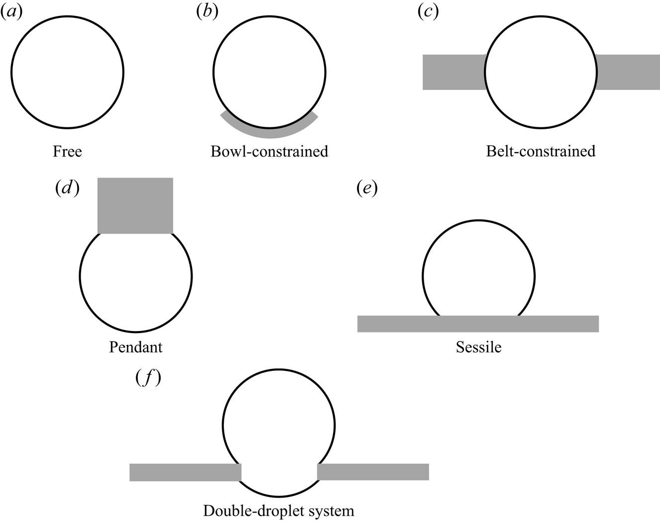
Use of (1.1) requires that the oscillating drop is somehow freely suspended in space, e.g. in a microgravity environment or in a levitator (Trinh & Wang Reference Trinh and Wang1982; Trinh, Zwern & Wang Reference Trinh, Zwern and Wang1982; Barmatz et al. Reference Barmatz, Trinh, Wang, Elleman and Jacobi1983). To circumvent this requirement and for a number of other reasons (see below), many researchers have more recently begun to analyse oscillations of droplets that are supported or constrained by a solid substrate (figure 1). Thus, increasing attention has been paid in recent years to the oscillations of globular drops constrained by solid spherical bowls (Strani & Sabetta Reference Strani and Sabetta1984, Reference Strani and Sabetta1988), belts (Bostwick & Steen Reference Bostwick and Steen2013a,Reference Bostwick and Steenb) and rings (Bostwick & Steen Reference Bostwick and Steen2009; Ramalingam & Basaran Reference Ramalingam and Basaran2010; Prosperetti Reference Prosperetti2012; Ramalingam, Ramkrishna & Basaran Reference Ramalingam, Ramkrishna and Basaran2012) and also pendant as well as sessile drops of arbitrary equilibrium shapes hanging from tubes or rods and/or sitting on planar solid substrates (Basaran & DePaoli Reference Basaran and DePaoli1994; Wilkes & Basaran Reference Wilkes and Basaran1997, Reference Wilkes and Basaran1999; Lyubimov, Lyubimova & Shklyaev Reference Lyubimov, Lyubimova and Shklyaev2006). The interest in oscillations of supported and constrained drops has continued to grow not only because such problems are physically interesting and mathematically challenging but also because they are of great practical importance in separations, mass transfer, measurement of dynamic surface tension, determination of intrinsic time scales of viscoelastic fluids and optics (Scott & Wham Reference Scott and Wham1988, Reference Scott and Wham1989; Harris, Scott & Byers Reference Harris, Scott and Byers1992; Ptasinski & Kerkhof Reference Ptasinski and Kerkhof1992; Zhang, Harris & Basaran Reference Zhang, Harris and Basaran1994; López & Hirsa Reference López and Hirsa2008; Brenn & Teichtmeister Reference Brenn and Teichtmeister2013). These fundamental studies have provided much insight into the effect of the constraint and its ramifications on the dynamical competition between inertial and surface tension forces among others. In particular, constraining a spherical drop as in the case of a capillary switch (CS) or a double-droplet system (DDS) where a portion of the drop protrudes above and a portion of it hangs below a liquid filled circular hole of small depth in a solid plate gives rise to a new mode of oscillation that consists primarily of COM motion which is disallowed in the case of free drops (Bostwick & Steen Reference Bostwick and Steen2009; Ramalingam & Basaran Reference Ramalingam and Basaran2010; Prosperetti Reference Prosperetti2012; Ramalingam et al. Reference Ramalingam, Ramkrishna and Basaran2012).
Often studied physical configurations involving oscillating drops. (a) A free drop that is surrounded by an exterior fluid that is dynamically either passive or active. (b) A drop that is constrained by a spherical solid bowl or cap. (c) A drop that is constrained by a solid belt. Here, the intersection of the solid belt and the liquid is a section of sphere. In the limit as the thickness of the belt tends to zero, the system reduces to a ring constrained drop (RCD). A RCD is also referred to as a drop constrained at an azimuth or a drop that is pinned along a latitude. (d) Pendant drop: a drop that typically hangs from a tube or a solid rod but also sometimes from a solid plate. (e) Sessile drop: a drop that typically sits on a solid plate. (f) A DDS or a CS. Here, fluid overfills a circular cylindrical hole in a solid plate so that part of it protrudes above the plate and part of it below it. In the limit as the plate thickness and hence the hole depth tends to zero, the system reduces to a ring constrained drop (see panel (c), above); in this paper, the system is a RCCD.

While all of the aforementioned single and DDSs described above exhibit stable oscillations when subjected to small-amplitude perturbations, drops can be linearly unstable if they are subjected to an external electric field (Taylor Reference Taylor1964; Brazier-Smith Reference Brazier-Smith1971; Miksis Reference Miksis1981; Adornato & Brown Reference Adornato and Brown1983; Basaran & Scriven Reference Basaran and Scriven1989a, Reference Basaran and Scriven1990; Basaran & Wohlhuter Reference Basaran and Wohlhuter1992; Wohlhuter & Basaran Reference Wohlhuter and Basaran1992, Reference Wohlhuter and Basaran1993) or are charged (Rayleigh Reference Rayleigh1882; Tsamopoulos & Brown Reference Tsamopoulos and Brown1984; Tsamopoulos, Aklas & Brown Reference Tsamopoulos, Aklas and Brown1985; Basaran & Scriven Reference Basaran and Scriven1989b). If an inviscid free drop is a perfectly conducting fluid bearing total charge  $Q$ that is surrounded by a perfectly insulating gas of permittivity
 $\epsilon _e$, it was shown in a celebrated paper by Rayleigh (Reference Rayleigh1882) that such a drop undergoes linear oscillations at frequencies given by
 \begin{equation} \varOmega_n^2 = n(n-1)(n+2)\frac{\sigma}{\rho R^3} \left[ 1 - \frac{Q^2}{(n+2)16{\rm \pi}^2 \epsilon_e \sigma R^3}\right]. \end{equation}
A comparison of (1.1) and (1.2) makes clear that the frequency of oscillation decreases as drop charge increases. More importantly, for each mode of oscillation, the oscillation frequency vanishes at a critical value of the total charge given by  $Q_{R}=\sqrt {(n+2)16{\rm \pi} ^2 \epsilon _e \sigma R^3}$. As the drop shape varies temporally as
 $\textrm {e}^{\textrm {i} \varOmega _n t}$, where
 $t$ is time, the dynamics which is oscillatory and stable when
 $Q< Q_R$ gives way to instability and exponential growth in time of the imposed perturbation when
 $Q>Q_R$. Instability occurs first for the lowest mode of oscillation, i.e. for
 $n=2$. The corresponding lowest value of charge for instability is the celebrated Rayleigh limit for which
 $Q_R \equiv \sqrt {64{\rm \pi} ^2 \epsilon _e \sigma R^3}$.
Although stable oscillations and instability of electrified drops have been studied for free drops (Tsamopoulos & Brown Reference Tsamopoulos and Brown1984; Feng & Beard Reference Feng and Beard1990; Basaran et al. Reference Basaran, Patzek, Benner and Scriven1995) as well as pendant and/or sessile drops (DePaoli et al. Reference DePaoli, Basaran, Feng and Scott1995), systematic investigations of the effect of constraints on such drops has heretofore been lacking. Unfortunately, the absence of a rigorous theoretical framework on oscillations of electrified constrained drops or bubbles is proving to be a limiting factor as a number of methods have been proposed recently such as that for inferring protein or surfactant adsorption from the oscillation frequency of charge-bearing constrained bubbles (Brocca et al. Reference Brocca, Saponaro, Introini, Rondelli, Pannuzzo, Raciti, Corti and Raudino2019) where a better fundamental understanding of the underlying oscillatory dynamics would be of great value. Motivated by this gap in the literature, we investigate in this paper the linear oscillations of a ring-constrained charged drop (RCCD). The analysis and results presented herein constitute the judicious amalgamation and extension of the classic work on isolated charged drops by Rayleigh (Reference Rayleigh1882) and the recent studies of constrained but neutral or uncharged drops by Bostwick & Steen (Reference Bostwick and Steen2009) and Ramalingam et al. (Reference Ramalingam, Ramkrishna and Basaran2012).
The manuscript is organized as follows. Section 2 presents the equations and boundary conditions governing the dynamics of a perfectly conducting, inviscid fluid undergoing incompressible flow, the base state solution that describes the equilibrium state of the RCCD before it is subjected to disturbances, and the linearization of the equations governing the perturbations. The linearized equations lead directly to a second-order integro-differential equation which is simplified into an eigenvalue problem using a linear operator formalism. Solutions to the eigenvalue problem which satisfy the constraints are uncovered in § 3 using a modified Rayleigh–Ritz method. The implications of pinning the drop at an azimuth and constraining the total charge to remain invariant on the oscillation characteristics of the lowest modes of oscillation are then discussed in § 4. Concluding remarks and a detailed road map for some possible avenues of future research bring the paper to a close in § 5.
2. Mathematical formulation
2.1. Governing equations
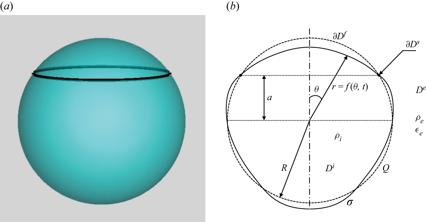
The system (figure 2) is isothermal: it consists of a drop that is pinned by a solid circular ring of vanishingly small thickness and the fluid that lies exterior to the drop. Throughout this paper, the dynamics is taken to be axisymmetric. In what follows,  $i$ (interior or drop) and
 $e$ (exterior) are used as subscripts and superscripts to delineate material properties and field variables in these two fluids. Both interior and exterior fluids are taken to be inviscid and incompressible with constant densities
 $\rho _i$ and
 $\rho _e$, respectively. Furthermore, the fluids both inside and outside the drop are assumed to undergo irrotational or potential flow. The drop fluid and the constraining ring are perfectly conducting while the exterior is a perfectly insulating fluid with constant permittivity
 $\epsilon _e$. The interface or free surface separating the two fluids has constant surface (interfacial) tension
 $\sigma$. Moreover, the surface of the constrained drop is charged. As the drop fluid and the ring are perfect conductors and the surrounding fluid a perfect insulator, the total amount of charge
 $Q$ remains invariant throughout the dynamics. Here, the effect of gravity is neglected so that the equilibrium shape of the RCCD is a sphere of radius
 $R$.
A ring constrained drop bearing total charge  $Q$. (a) Perspective view showing the drop and the solid ring constraint. (b) Cross-sectional view and definition sketch. The drop's shape is denoted by the dashed line in its unperturbed state and a solid line in its perturbed state. The solid constraint
 $\partial D^s$, which is a latitudinal circle, is denoted by the two points or small black circles in this cross-sectional view.

As the base state is a sphere, it is convenient to use a spherical polar coordinate system  $(r,\theta ,\psi )$ where
 $r$,
 $\theta$ and
 $\psi$ (
 $r \ge 0$,
 $0 \le \theta \le {\rm \pi}$, and
 $0 \le \psi < 2{\rm \pi}$) stand for the radial coordinate, cone angle and the polar angle, respectively, with its origin located at the centre of the unperturbed drop. Because of axisymmetry, the problem domain consists of the
 $(r, \theta )$-plane as shown in figure 2. In this coordinate system, the solid circle of contact (or pinning location) is placed at an azimuthal angle
 $\alpha \ (0 \le \alpha \le {\rm \pi})$ or axial distance
 $a=R\cos \alpha \ (R \ge a \ge -R)$ measured from the equatorial midplane of the unperturbed drop. The free surface separating the two phases is located at
 $r=f(\theta ,t)$ where
 $t$ denotes time. The domains corresponding to the drop's interior, its exterior, the free surface and the pinning location where the solid is located are denoted by
 $D^i$,
 $D^e$,
 $\partial D^f$ and
 $\partial D^s$, respectively, and defined mathematically by
 $$\begin{gather} D^i \equiv \{(r,\theta) \mid 0 \leq r \leq f, 0 \leq \theta \leq {\rm \pi}\}, \end{gather}$$
 $$\begin{gather}D^e \equiv \{(r,\theta) \mid f \leq r \leq \infty, 0 \leq \theta \leq {\rm \pi}\}, \end{gather}$$
 $$\begin{gather}\partial D^f \equiv \{(r,\theta) \mid r=f, 0 \leq \theta \leq {\rm \pi}, \theta \neq \alpha\}, \end{gather}$$
 $$\begin{gather}\partial D^s \equiv \{(r,\theta) \mid r=R, \theta = \alpha\}. \end{gather}$$
As both fluids undergo irrotational flow, fluid velocity  $\boldsymbol {v} \equiv -\boldsymbol {\nabla } \varPhi$ where
 $\varPhi$ is the velocity potential. Since the fluids are incompressible (
 $\boldsymbol {\nabla } \boldsymbol {\cdot } \boldsymbol {v} = 0$), the velocity potential both inside and outside the drop is governed by Laplace's equation,
 \begin{equation} \nabla^2 \varPhi = 0 \text{ in } D^i \text{ and } D^e. \end{equation}
In potential flow of an incompressible fluid, the momentum equation reduces to a scalar equation (Bernoulli's equation) governing the pressure,  $P$,
 \begin{equation} P = \rho \left(\frac{\partial \varPhi}{\partial t} - \frac{1}{2} (\boldsymbol{\nabla} \varPhi)^2\right) \text{ in } D^i \text{ and } D^e. \end{equation}
The electric field  $\boldsymbol {E}$ inside the conducting drop vanishes but that in the exterior fluid
 $\boldsymbol {E} \equiv - \boldsymbol {\nabla } V$ where
 $V$ is the electrostatic potential. Since
 $\boldsymbol {\nabla } \times \boldsymbol {E} = \mathbf 0$ and
 $\boldsymbol {\nabla } \boldsymbol {\cdot } (\epsilon _e \boldsymbol {E}) = 0$, the electrostatic potential too is governed by Laplace's equation,
 \begin{equation} \nabla^2 V = 0 \text{ in } D^e. \end{equation}
The aforementioned equations are subject to the following boundary conditions. Two of these, the kinematic and traction (normal stress) boundary conditions, are the counterparts at the free surface of the mass and momentum balances in the bulk fluids
 $$\begin{gather} \left.\frac{\textrm{D}}{\textrm{D}t} ( r-f(\theta,t) ) \right|_{r=f(\theta,t)} = 0 \text{ on } \partial D^f, \end{gather}$$
 $$\begin{gather}P^i - P^e+ \tfrac{1}{2}\epsilon_e (\boldsymbol{n} \boldsymbol{\cdot} -(\boldsymbol{\nabla} V))^2={-}2\mathcal{H}\sigma \text{ on } \partial D^f, \end{gather}$$
where  $-2\mathcal {H}$ is the twice mean curvature of and
 $\boldsymbol {n}$ is the unit normal to the free surface
 \begin{equation} \boldsymbol{n}=\frac{[f\boldsymbol{e}_r - (\partial f/\partial \theta)\boldsymbol{e}_\theta]}{[f^2 +(\partial f/\partial \theta)^2]^{1/2}}, \end{equation}
where  $\mathbf {e}_r$ and
 $\mathbf {e}_{\theta }$ are the unit vectors in the
 $r$- and
 $\theta$-directions. The pinning location is fixed and is impenetrable; therefore (cf. Bostwick & Steen Reference Bostwick and Steen2009),
 \begin{equation} f(\alpha, t) = R \quad \text{and} \quad \boldsymbol{e}_r \boldsymbol{\cdot} \boldsymbol{\nabla} \varPhi = 0 \text{ on } \partial D^s. \end{equation}
The fluid velocity is bounded at the origin and vanishes at infinity,
 \begin{equation} \frac{\partial\varPhi}{\partial r} \neq \infty \text{ at } r=0 \quad \text{and} \quad \varPhi \to 0 \text{ as } r \to \infty. \end{equation}
As the drop fluid and the solid constraint pinning the drop are perfect conductors, the tangential component of the electric field is zero along the surface separating the interior and exterior fluids
 \begin{equation} \boldsymbol{t} \boldsymbol{\cdot} -\boldsymbol{\nabla} V = 0 \text{ on } \partial D^f \text{ and } \partial D^s, \end{equation}
where  $\boldsymbol {t}$ denotes the unit tangent. This condition is equivalent to requiring that the boundary
 $\partial D^f \cup \partial D^s$ separating the interior and exterior fluids is an equipotential surface. However, although the electric potential is spatially uniform on
 $\partial D^f \cup \partial D^s$, its value may be a function of time (see below). At large distances from the RCCD, the electric potential must asymptotically tend to zero
 \begin{equation} V \rightarrow 0 \text{ as } r \rightarrow \infty. \end{equation}
Additionally, the field variables ( $f, \varPhi , V, P$) must obey conditions of axisymmetry at
 $\theta = 0$ and
 ${\rm \pi}$.
As drop volume and charge are fixed, both the drop volume and the total charge must remain invariant for all time,
 $$\begin{gather} \int \, \textrm{d} {V} = \frac{4{\rm \pi}}{3}R^3, \end{gather}$$
 $$\begin{gather}\left.\int (\boldsymbol{n} \boldsymbol{\cdot} -(\boldsymbol{\nabla} V))\right|_{r=f(\theta,t)} \, \textrm{d} {S} = \frac{Q}{\epsilon_e}, \end{gather}$$
where the first integral is over the volume and the second integral over the surface of the RCCD. The latter integral constraint also determines the value of the electric potential at the free surface and the pinning location.
2.2. Equations governing the perturbations and normal mode analysis
The equilibrium state in which a RCCD is perfectly spherical in shape and where the fluids both inside and outside the drop are quiescent is an exact solution of the governing system of equations and boundary conditions. For this base state, the electric potential exterior to the drop decays as  $1/r$ and is given by
 $Q/4{\rm \pi} \epsilon _e r$. Furthermore, in this quiescent state, the pressure in both fluids is constant, with the pressure in the drop exceeding the external pressure by
 $2\sigma /R - Q^2/32{\rm \pi} ^2\epsilon _e R^4$.
To analyse the dynamics that ensues when the aforementioned base state is perturbed, the field variables, i.e. the velocity potential  $\varPhi (r,\theta ,t)$, pressure
 $P(r,\theta ,t)$, electric potential
 $V(r,\theta ,t)$ and drop shape
 $r=f(\theta ,t)$, are expressed as their base state or unperturbed state values, viz.
 $\varPhi _0$,
 $P_0$,
 $V_0$ and
 $R$, plus a perturbation,
 $$\begin{gather} \varPhi = \varPhi_0 + \varPhi', \end{gather}$$
 $$\begin{gather}P = P_0 + P', \end{gather}$$
 $$\begin{gather}V = V_0 + V', \end{gather}$$
 $$\begin{gather}f = R + \eta, \end{gather}$$
where  $\varPhi '$,
 $P'$,
 $V'$ and
 $\eta$ are small perturbations.
The small perturbations are then expressed using normal mode analysis (Chandrasekhar Reference Chandrasekhar1961) as
 $$\begin{gather} \varPhi'=\phi(r,\theta)\, \textrm{e}^{\textrm{i} \omega t}, \end{gather}$$
 $$\begin{gather}V'=v(r,\theta)\, \textrm{e}^{\textrm{i} (\omega t + {\rm \pi}/2)}, \end{gather}$$
 $$\begin{gather}P'=p(r,\theta)\, \textrm{e}^{\textrm{i} (\omega t + {\rm \pi}/2)}, \end{gather}$$
 $$\begin{gather}\eta=z(\theta)\, \textrm{e}^{\textrm{i} (\omega t + {\rm \pi}/2)}, \end{gather}$$
where the reduced functions  $\phi$,
 $v$,
 $p$ and
 $z$ are the amplitudes of the small perturbations and
 $\omega$ is the frequency. The phase difference
 ${\rm \pi} /2$ in the expressions for the perturbations in electric potential, pressure and interface deflection ensures that the boundary conditions are satisfied.
The linearized system of equations governing the perturbations can be rewritten in terms of the reduced functions or the amplitudes  $\phi (r,\theta )$,
 $v(r,\theta )$ and
 $z(\theta )$ as
 $$\begin{gather} \nabla^2 \phi = 0 \text{ in } D^i \text{ and } D^e, \end{gather}$$
 $$\begin{gather}\nabla^2 v = 0 \text{ in } D^e, \end{gather}$$
 $$\begin{gather}p = \rho \omega \phi \text{ in } D^i \text{ and } D^e, \end{gather}$$
 $$\begin{gather}\phi_r = \omega z \text{ on } \partial D^f, \end{gather}$$
 $$\begin{gather}\phi_r = 0 \text{ on } \partial D^s, \end{gather}$$
 $$\begin{gather}v_{\theta} = \frac{Q}{4{\rm \pi}\epsilon_e R^2}z_{\theta} \text{ on } \partial D^f \text{ and } \partial D^s, \end{gather}$$
 $$\begin{gather}\omega(\rho_i\phi^i - \rho_e\phi^e) + \frac{Q^2}{16 {\rm \pi}^2 \epsilon_e R^5}(v_r - 2z) ={-}\frac{\sigma}{R^2}\left( \frac{(\sin \theta z_{\theta})_{\theta}}{\sin \theta} + 2z \right) \text{ on } \partial D^f, \end{gather}$$
 $$\begin{gather}\int_0^{\rm \pi} z \sin \theta \, \textrm{d} {\theta} = 0, \end{gather}$$
 $$\begin{gather}\int_0^{\rm \pi} v_r|_{r=R} \sin \theta \, \textrm{d} {\theta} = 0, \end{gather}$$
where subscripts  $r$ and
 $\theta$ denote the partial derivatives with respect to those variables. As situations in which the electric potential of the surface of a perfect conductor is uniform but may vary with time are less common than ones in which the potential is constant, we present in Appendix A two alternate ways of deriving equation (2.30).
The above set of equations governing  $\phi$ and
 $v$ can be recognized as the standard Neumann problem. Making the substitution
 $x=\text {cos}\,\theta $, the solution of (2.25) and (2.26) subject to boundedness at the poles, and (2.28) and (2.30), respectively, are
 $$\begin{gather} \phi^i(r,\theta)=\omega R \left(\phi_0 + \sum_{k=1}^{\infty} \frac{\phi_k}{k}\frac{r^k}{R^k} p_k(x) \right), \end{gather}$$
 $$\begin{gather}\phi^e(r,\theta)={-}\omega R \left(\sum_{k=1}^{\infty} \frac{\phi_k}{k+1}\frac{R^{k+1}}{r^{k+1}} p_k(x) \right), \end{gather}$$
 $$\begin{gather}v(r,\theta)=\frac{Q}{4{\rm \pi}\epsilon_e R^2} \left(\sum_{k=1}^{\infty} \phi_k \frac{R^{k+1}}{r^{k+1}} p_k(x) \right), \end{gather}$$
where  $p_k(x)$ is the
 $k$th normalized Legendre polynomial, and the coefficients
 $\phi _k$ are given by
 \begin{equation} \phi_k= \langle z, p_k\rangle , \end{equation}
with the inner product of two arbitrary functions  $g$ and
 $h$ defined as
 \begin{equation} \langle g,h\rangle = \int_{{-}1}^1 gh \, \textrm{d} {x}. \end{equation}
Substituting equations ((2.34)–(2.36)) into (2.31) yields a second-order integro-differential equation governing the oscillation frequency,  $\omega$,
 \begin{align} \frac{\omega^2 \rho_i R^3}{\sigma}\left(\sum_{k=1}^{\infty}\beta_k \phi_k p_k \right) ={-}[(1-x^2)z_x]_x -2z - \frac{Q^2}{16{\rm \pi}^2\epsilon_e\sigma R^3}\left(\sum_{k=1}^{\infty}(k+1)\phi_k p_k - 2z\right),\end{align}
where
 \begin{equation} \beta_k = \frac{1}{k} + \frac{\rho_e}{\rho_i}\frac{1}{k+1}. \end{equation}
Solutions of the dispersion equation (see (2.39)) need to be calculated subject to the volume constraint, boundedness conditions at the poles, and vanishing of the shape perturbation at the solid contact,
 $$\begin{gather} \int_{{-}1}^{1} z(x) \, \textrm{d} {x} = 0, \end{gather}$$
 $$\begin{gather}z(\pm1) < \infty, \end{gather}$$
 $$\begin{gather}z(a) = 0; \quad a = \cos \alpha. \end{gather}$$
Equation (2.39) can be conveniently written as a linear operator eigenvalue problem
 \begin{equation} \lambda \boldsymbol{M}z = (\boldsymbol{L} - \boldsymbol{H})z,\end{equation}
where
 $$\begin{gather} \boldsymbol{L}\bullet{\equiv} -\frac{\partial}{\partial x}\left[(1-x^2) \frac{\partial \bullet}{\partial x} \right] - 2\bullet, \end{gather}$$
 $$\begin{gather}\boldsymbol{H}\bullet{\equiv} \chi^2\left(\sum_{k=1}^\infty (k+1)\langle \bullet,p_k\rangle p_k - 2\bullet \right), \end{gather}$$
 $$\begin{gather}\boldsymbol{M}\bullet{\equiv} \langle \bullet, p_0\rangle + \sum_{k=1}^\infty \beta_k\langle \bullet,p_k\rangle p_k, \end{gather}$$
 $$\begin{gather}\lambda \equiv \frac{\omega^2 \rho_i R^3}{\sigma}, \end{gather}$$
 $$\begin{gather}\chi^2 \equiv \frac{Q^2}{16 {\rm \pi}^2 \epsilon_e \sigma R^3}. \end{gather}$$
Given the boundary conditions in ((2.41)–(2.43)) and the inner product defined by (2.38), operators  $\boldsymbol {L}$,
 $\boldsymbol {H}$ and
 $\boldsymbol {M}$ are self-adjoint. Solutions to (2.44) that satisfy ((2.41)–(2.43)) are eigenfunctions that describe the shape of a constrained drop bearing dimensionless charge
 $\chi$ undergoing periodic oscillations with dimensionless frequency
 $\sqrt {\lambda }$.
3. Minimization method
While many methods have been employed to solve analogues of (2.39), here we follow the minimization method described by Ramalingam et al. (Reference Ramalingam, Ramkrishna and Basaran2012). An overview of these different methods and a comparison with that used here can be found in Appendix B. As is the case with all of these methods, we construct eigensolutions to (2.39). The objective in solving this eigenvalue problem is to find the eigenvalues of the operator  $\boldsymbol {T} = \boldsymbol {M}^{-1} (\boldsymbol {L}-\boldsymbol {H})$. It can be shown that the operator
 $\boldsymbol {T}$ is self-adjoint (Ramkrishna & Amundson Reference Ramkrishna and Amundson1985) with respect to the inner product defined in
 $\mathcal {L}^2 [-1,1]$ by
 \begin{equation} \langle u,w\rangle _M \equiv \langle \boldsymbol{M}u,w\rangle , \end{equation}
where  $\langle \, , \, \rangle$ is the inner product defined by (2.38). Operators
 $\boldsymbol {L}-\boldsymbol {H}$ and
 $\boldsymbol {M}$ have eigenvalues of
 $\gamma _j = (j-1)(j+2) - \chi (j-1)$ and
 $\beta _j$ (under the normal inner product), respectively, with the normalized Legendre polynomial
 $p_j$ as the corresponding eigenfunction. Therefore, the linear operator
 $\boldsymbol {T}$ has eigenvalues
 $\gamma _j/\beta _j$ with
 $p_j$ as the corresponding eigenfunction. The Rayleigh–Ritz form of (2.44) is
 \begin{equation} \lambda \boldsymbol{M}z = (\boldsymbol{L}-\boldsymbol{H})z \equiv \text{Min}[\langle \boldsymbol{T}z,z\rangle _M - \lambda(\langle z,z\rangle _M-1) ]. \end{equation}
The ring constraint is introduced into this formulation through the use of an additional Lagrange multiplier  $\nu$. The eigenvalue
 $\lambda$ can then be determined by minimization of the objective function as
 \begin{equation} \text{Min}[\langle \boldsymbol{T}z,z\rangle _M - \lambda(\langle z,z\rangle _M-1) - \nu z(a)]. \end{equation}
The objective function is simplified by expanding  $z(x)$ in terms of the normalized Legendre polynomials,
 \begin{equation} z(x) = \sum_{j=1}^N c_j p_j(x). \end{equation}
Substitution of this expansion into the minimization problem then yields
 \begin{equation} \text{Min}\left [\sum_{j=1}^N c^2_j\gamma_j - \nu \sum_{j=1}^N c_j p_j(a) - \lambda \left ( \sum_{j=1}^N c^2_j\beta_j - 1 \right ) \right ]. \end{equation}
Upon differentiation with respect to  $c_k$ and setting the result equal to zero, it is found that
 \begin{equation} c_k = \frac{\nu p_k(a)}{2 ( \gamma_k - \lambda \beta_k )}. \end{equation}
From the normalization condition  $\langle z,z\rangle _M =1$, it follows that
 \begin{equation} \nu = \frac{2}{\sqrt{\displaystyle \sum_{k=1}^N \frac{\beta_k p^2_k(a)}{( \gamma_k - \lambda \beta_k )^2}}}. \end{equation}
Substitution of (3.6) and (3.7) into the pinning condition ( $z(a)=0$) at last yields the following implicit equation that can be used for determining the eigenvalues:
 \begin{equation} f(\lambda) \equiv \sum_{k=1}^{N} \frac{p^2_k(a)}{\gamma_k - \lambda \beta_k} = \sum_{k=1}^{N} \frac{p^2_k(a)}{ \beta_k(\varOmega^2_k - \lambda )} = 0. \end{equation}
Here,  $\varOmega ^2_k$ (
 $\equiv \gamma _k/\beta _k$) is the Rayleigh frequency given by (1.2). In this paper, (3.8) is solved using the Newton–Raphson method. In the remainder of the paper, the solutions that are reported have been obtained with
 $N=100$ and when
 $\rho _e/\rho _i \ll 1$.
4. Results
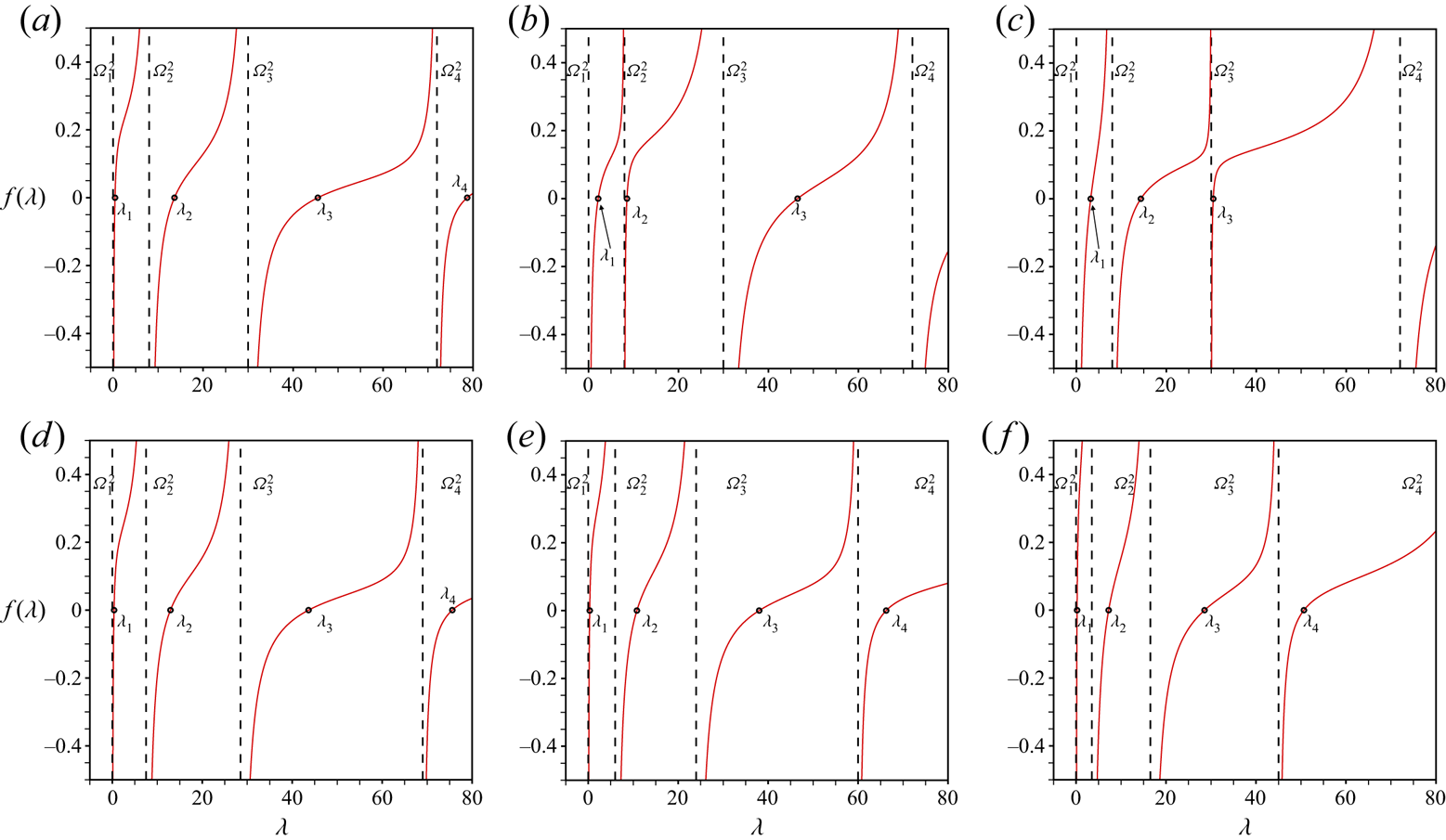
Figure 3(a–c) shows the variation of  $f(\lambda )$ with
 $\lambda$ for three uncharged drops (
 $\chi = 0$) that are constrained at different pinning locations. Figure 3(d–f) shows the variation of
 $f(\lambda )$ with
 $\lambda$ for three charged drops (
 $\chi \ne 0$) that are all constrained at the same pinning location. It can be readily appreciated from the form of (3.8) and figure 3 that the function
 $f(\lambda )$ has a number of noteworthy features. First,
 $f(\lambda )$ has a countably infinite number of poles. These poles are located at the square of each Rayleigh frequency, viz.
 $\varOmega ^2_k$. Second,
 $f(\lambda )$ varies monotonically and strictly increases with
 $\lambda$ between any two consecutive Rayleigh frequencies. Therefore, there exists one and only one zero of
 $f(\lambda )$ between two successive poles. Each of these zeros is an eigenvalue
 $\lambda$. Thus, the frequency of the
 $j$th mode of oscillation is
 $\sqrt {\lambda _j}$, where
 $\lambda _j$ are the roots of
 $f(\lambda _j) = 0$: each root is such that
 $\varOmega ^2_j \leq \lambda _j \leq \varOmega ^2_{j+1}$ where
 $\varOmega ^2_j=\varOmega ^2_j(\chi )$ and
 $\lambda _j=\lambda _j (a,\chi )$. In other words, unlike free drop oscillations, here the mode of oscillation is defined only by the frequency and the link between mode and shape perturbation is lost (Bostwick & Steen Reference Bostwick and Steen2009; Ramalingam et al. Reference Ramalingam, Ramkrishna and Basaran2012). The shape of the perturbed drop undergoing vibrations in the
 $j$th mode of oscillation can be determined by substituting
 $\lambda _j$ into (3.7), (3.6) and (3.4). Now that the nature of the solutions to (3.8) and the definition of the oscillation mode have been established, attention will be turned to carrying out a detailed examination of the effect of pinning in both the absence and presence of charge.
(a–c) Variation of  $f(\lambda )$ with
 $\lambda$ (3.8) for uncharged drops (
 $\chi =0$) that are constrained at three different pinning locations: (a)
 $a=0.25$; (b)
 $a=0.5$; (c)
 $a=0.75$. (d–f) Variation of
 $f(\lambda )$ with
 $\lambda$ (3.8) for charged drops (
 $\chi \ne 0$) of increasing charge but which are constrained at the same pinning location of
 $a=0.25$: (d)
 $\chi =0.5$; (e)
 $\chi =1.0$; (f)
 $\chi =1.5$. Solid red curves denote the function
 $f(\lambda )$, dashed black vertical lines denote the poles
 $\varOmega ^2_k$, and open black circles denote the zeros of
 $f(\lambda )$ which correspond to the eigenvalues
 $\lambda _k$ or the squares of the eigenfrequencies of oscillation.

4.1. Effect of pinning
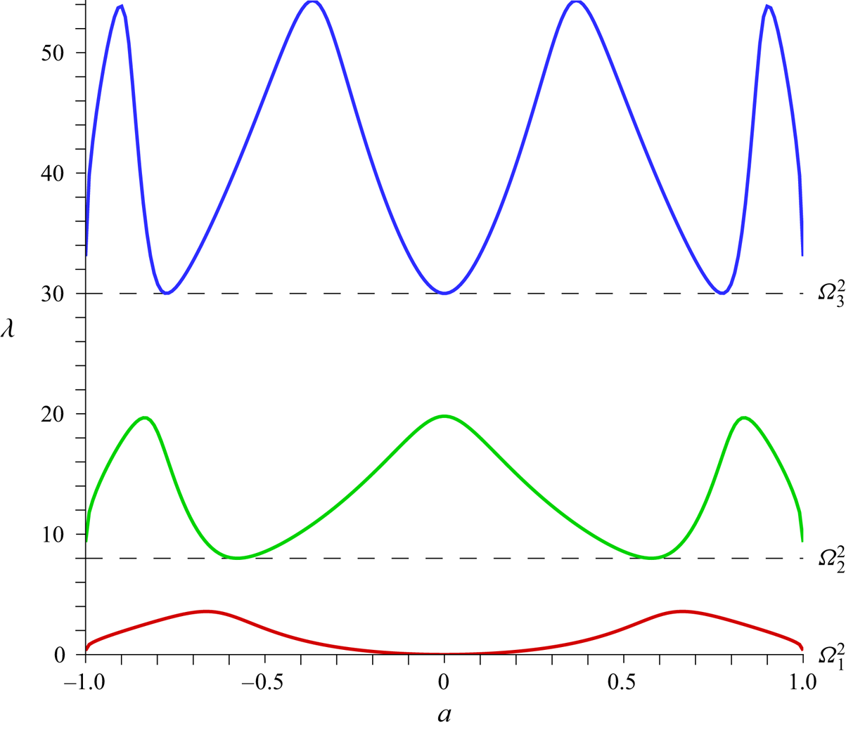
In order to get a better handle on the physics of constraining a charged drop, it is vital that we first discuss and review briefly the main consequences of the effect of pinning in the absence of charge (see also Bostwick & Steen (Reference Bostwick and Steen2009), Ramalingam et al. (Reference Ramalingam, Ramkrishna and Basaran2012) and Prosperetti (Reference Prosperetti2012)). Moreover, the results presented in this subsection also provide testament to the accuracy of the approach used in this paper to compute the eigenvalues and hence the eigenfrequencies of oscillation of constrained drops. Figure 4 shows solutions to (3.8) for an uncharged drop ( $\chi =0$) and a range of pinning locations for the first, second and third modes of oscillation. First, this figure makes plain that the curves depicting oscillation frequency versus
 $a$ for every mode is symmetric about pinning the drop at the equator (
 $a=0$) – a result that accords with intuition in the absence of gravity. Breaking this symmetry may be useful in future applications involving constrained drops, a point that is returned to in the conclusions.
Variation of the square of the dimensionless eigenfrequency  $\lambda$ with pinning location
 $a$ of an uncharged constrained drop (
 $\chi =0$) for the first (bottom red curve), second (middle green curve) and third (top blue curve) modes of oscillation. It is easily seen that each curve of
 $\lambda$ versus
 $a$ for the
 $j$th mode of oscillation has
 $j$ minima and
 $j+1$ local maxima. As discussed in the text, the value of the oscillation frequency of a constrained drop at each minimum is exactly the square of the Rayleigh frequency
 $\varOmega ^2_j$ for a free drop (black dashed lines).

Second, unlike free drops and as discussed in the introduction, the presence of the constraint has given rise to a first mode of oscillation. Indeed, in their pioneering work, Bostwick & Steen (Reference Bostwick and Steen2009) showed that this mode is associated primarily with the COM motion of constrained drops, an insight that is of significant value in improving the understanding of pinch-off or breakup in applications such as ink jet printing (Basaran, Gao & Bhat Reference Basaran, Gao and Bhat2013; Castrejón-Pita et al. Reference Castrejón-Pita, Baxter, Morgan, Temple, Martin and Hutchings2013).
Third, another important realization obtained from analysis of situations in which the constrained drop is uncharged is that varying the pinning location can greatly alter the frequency of oscillation. For example, as shown in figure 4, the second mode of oscillation for an uncharged drop pinned at  $a\approx 0.8$ is more than double the frequency if the drop were instead pinned at
 $a\approx 0.6$. Moreover, extrema in frequency are encountered for each mode of oscillation as pinning location is varied. Specifically, the
 $j$th mode of oscillation has
 $j$ frequency minima and
 $j+1$ frequency maxima. Furthermore, these frequency minima for each mode always correspond to the square of the Rayleigh frequency. While it might appear strange and unexpected that the frequency of a pinned drop and that of a free drop could be identical, the equality of the frequencies can be readily understood by considering the nature of the shape perturbations for free drops. For example, the transient shape of a free drop undergoing second-mode oscillations is given by
 \begin{equation} f(\theta,t) = R + \epsilon p_2(x)\, \textrm{e}^{\textrm{i} \varOmega_2 t + {\rm \pi}/2}, \end{equation}
where  $\epsilon \ll R$ is the amplitude of the shape perturbation that the drop is subjected to,
 $x \equiv \cos \theta$, and
 $\varOmega _2$ is the frequency of oscillation. The equality of the frequencies results because
 $p_2(x)$, the Legendre polynomial of order two, has two roots (at
 $x=\pm 1 /\sqrt {3}$) where the perturbation to the spherical base profile vanishes for all time. Consequently, pinning the drop at axial locations corresponding to these roots has no effect whatsoever, and the constrained and free oscillations are therefore dynamically identical. Since the constraint is satisfied ‘naturally’ at these locations, local minima are termed ‘natural’ pinning locations and, conversely, local maxima are referred to as ‘unnatural’ pinning locations.
4.2. Behaviour near the Rayleigh limit
A key result of inviscid linear stability analysis is identifying a set of parameters for which the oscillation frequency tends to zero and beyond which point stability may be lost. Uncharged free drops are always linearly stable as the frequency of oscillation is always real and non-zero. Charged free drops are linearly stable if the total charge is below the Rayleigh limit as the frequency of oscillation is real and non-zero. When drop charge  $Q$ equals that at the Rayleigh limit
 $Q_R$, the frequency of the second-mode of oscillation vanishes. When
 $Q$ exceeds
 $Q_R$, (1.2) shows that for the second-mode of oscillation, the two frequencies are imaginary and complex conjugates of one another. The root with the negative sign leads to exponential growth in time of small-amplitude disturbances or shape perturbations and hence instability.
As shown in figure 3 and discussed above, for RCCDs, each eigenvalue (square of the oscillation frequency) is bounded both above and below by the square of consecutive Rayleigh frequencies, e.g.  $\varOmega ^2_1=0 \leq \lambda _1 \leq \varOmega ^2_2(\chi ) \leq \lambda _2 \leq \varOmega ^2_3(\chi )$. As dimensionless charge
 $\chi$ increases, these bounds decrease as
 $\chi ^2$ and in the present formulation the Rayleigh limit (where
 $\varOmega ^2_2=0$) is obtained when
 $\chi =2$. Hence, by definition, the oscillation frequency of the first mode for a constrained drop must vanish when
 $\chi =2$ irrespective of pinning location
 $a$. Thus, while for free drops the second mode of oscillation has zero frequency and is known to have reached its limit of stability when
 $\chi =2$, for constrained drops it is the first mode of oscillation whose frequency vanishes when
 $\chi =2$.
4.3. Combined effect of arbitrary drop charge and varying pinning location
For free drops, the decrease in the frequency of each mode of oscillation is commensurate with the increase in drop charge: as  $\chi$ increases,
 $\varOmega ^2_j$ for the
 $j$th mode decreases as
 $\chi ^2$. In order to determine if the same holds true for constrained charged drops, it proves convenient to take advantage of the boundedness of the eigenvalues (squares of the frequencies) discussed above to rescale the oscillation frequency of the constrained charged drop as follows. The advantage of this rescaling is that it makes it straightforward to appreciate the combined effects of charge and constraint for a RCCD relative to a free charged drop. In particular, we seek to elucidate the changes in the first and second modes of oscillation en route to instability or in the limit as
 $\chi \to 2$. Thus, the rescaled frequency is defined as
 \begin{equation} \varLambda_j = \frac{\lambda_j - \varOmega^2_j}{\varOmega_{j+1}^2 - \varOmega_{j}^2} + (j-1). \end{equation}
For the  $j$th mode, the lower bound on the frequency corresponds to
 $\lambda _j \to \varOmega _j^2$ and upper bound on the frequency corresponds to
 $\lambda _j \to \varOmega _{j+1}^2$. In terms of the rescaled frequency, the lower and upper bounds are therefore given by
 $j-1$ and
 $j$. For a RCCD undergoing first-mode oscillations, the lower and upper bounds on the rescaled frequency are 0 and 1. The upper bound of one in this case corresponds to a free charged drop undergoing second-mode oscillations such that the square of its frequency of oscillation is
 $\varOmega _2^2$. For a RCCD undergoing second-mode oscillations, the lower and upper bounds on the rescaled frequency are 1 and 2. The lower bound of one in this case corresponds to a free charged drop undergoing second mode oscillations such that the square of its frequency of oscillation is
 $\varOmega _2^2$.
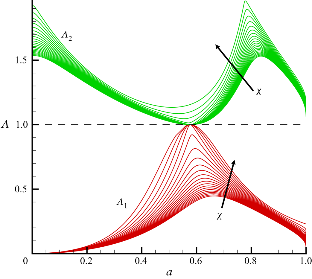
Figure 5 shows the variation of the rescaled frequency  $\varLambda _j$ for the first (red curves) and second (green curves) modes of oscillation of a RCCD with pinning location
 $a$ for several values of the dimensionless drop charge
 $\chi$. Here, symmetry of the dynamics about pinning at the equator is exploited and hence results for only
 $a>0$ are shown in the figure. While the shapes of the curves shown in figure 5 and those in figure 4 are qualitatively similar, the effect of charge is not manifested in identical manner for every pinning location. If the effect of charge was commensurate for all pinning locations, then it would be possible to rescale the oscillation frequencies or collapse them onto a single ‘master curve’ such that the dependence on
 $\chi$ can be removed. In other words, if charge had the same effect for each pinning location, then
 $\varLambda =\varLambda (a)$ and not
 $\varLambda =\varLambda (a,\chi )$ as can be seen in figure 5. Indeed, this fact is made plain by examining the variation of the local extrema for each mode with
 $\chi$. For the first mode of oscillation, the value of the frequency maximum grows relative to its lower bound and even approaches the upper bound for this mode. Moreover, the axial pinning location to which this maximum corresponds, the ‘unnatural’ pinning location, shifts towards the equator of the RCCD as dimensionless drop charge
 $\chi$ increases. This trend is also observed for the second mode of oscillation, but the shift in the ‘unnatural’ pinning location is only observed for
 $a \neq 0$. Moreover, according to the results shown in figure 5, the ‘natural’ pinning location for the second mode intriguingly exhibits a discontinuous behaviour. For values of the dimensionless drop charge
 $\chi$ below a certain particular value, the frequency of oscillation of a RCCD pinned at that location corresponds exactly to that of a free drop bearing the same charge. However, for values of
 $\chi$ above this critical value, the value of the frequency at that pinning location exceeds that of a free drop. Indeed, the value of the frequency minimum increases and the value of the pinning location decreases as
 $\chi$ continues to increase beyond this critical value. Clearly, further analysis is needed to shed light on this discontinuous behaviour.
Variation of the square of the rescaled oscillation frequency  $\varLambda _j$ (see (4.2)) of a RCCD with pinning location
 $a$ and dimensionless drop charge
 $\chi$ for the first (
 $\varLambda _1$, bottom red curves) and second (
 $\varLambda _2$, top green curves) modes of oscillation. The horizontal black dashed line (with ordinate value of one) corresponds to the frequency of oscillation of the second mode of a free charged drop (see (1.2)). For both modes of oscillation of a RCCD, arrows indicate the direction of increasing charge, with the uppermost curves corresponding to
 $\chi =1.99$ and the lowermost curves to
 $\chi =0$ (the results shown in figure 4).

4.4. Eigenvalue veering
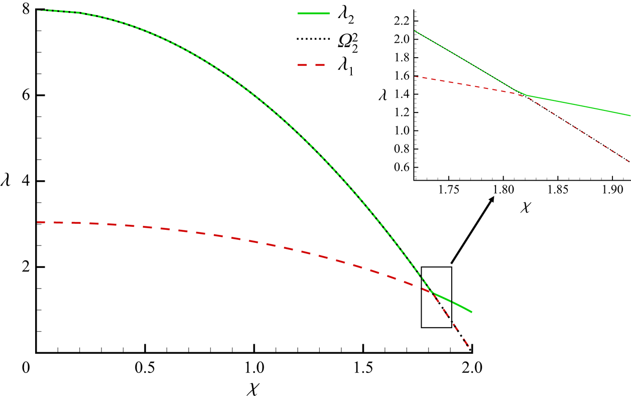
In order to investigate the discontinuous behaviour in the oscillation frequency reported in figure 5, we next focus on the variation with charge of the oscillation frequencies of the first and second modes for a drop constrained at the ‘natural’ pinning location of the second mode ( $a=1/\sqrt {3}$). Figure 6 shows that as dimensionless charge
 $\chi$ increases from zero, the square of the frequency of the second mode of oscillation of the constrained drop (
 $\lambda _2$, green curve) is identical to that of the free drop (
 $\varOmega _2^2$, black dashed curve). Furthermore, as
 $\chi$ further increases,
 $\lambda _2$ and
 $\varOmega _2^2$ approach the square of the oscillation frequency of the first mode (
 $\lambda _1$, red curve). When
 $\chi \approx 1.82$, these three quantities become nearly identical. Moreover, when
 $\chi > 1.82$,
 $\lambda _2$ and
 $\lambda _1$ veer apart such that thereafter the square of the frequency of the first mode of the constrained drop
 $\lambda _1$ is identical to
 $\varOmega _2^2$. Although the curve veering phenomenon displayed in figure 6 has almost never been mentioned in any of the classic papers on drop oscillations reviewed in the introduction, the topic has been of particular interest in the vibrations and acoustics community. One of the earliest observations of the veering phenomenon were reported by Claassen (Reference Claassen1962). Later, Leissa (Reference Leissa1974) provided further examples suggesting eigenvalue curve veering could be artificially induced by inadequate approximation of solutions. Perkins & Mote (Reference Perkins and Mote1986) provided an exact mathematical solution exhibiting curve veering. These authors demonstrated that modes in self-adjoint eigenvalue problems will always veer except in the limiting case of zero modal coupling. du Bois, Adhikari & Lieven (Reference du Bois, Adhikari and Lieven2009) provided a clear experimental demonstration of eigenvalue curve veering in a redundant truss system. Nevertheless, the existence of curve veering was recognized by Bostwick & Steen (Reference Bostwick and Steen2013a) who studied the oscillations of an uncharged inviscid drop constrained by a belt. These authors report that the eigenfrequencies exhibit ‘near crossings’ where two different modal shapes have nearly the same frequency. In their work, ‘near crossings’ are located by determining the set of parameters for which the volume displaced by one free surface is equivalent for two consecutive modes of oscillation. A commonality of all aforementioned works is that eigenvalues approach each other as a system parameter is varied. Naturally, we seek to understand first why the eigenvalues approach one another in this system and second, what the distinguishing physical characteristics are of the eigensolutions when the eigenvalues are nearly identical. To answer these questions, we turn to energy arguments. Let
 $z_i$ be the eigenfunction for the
 $i$th mode of oscillation with eigenvalue (square of the oscillation frequency)
 $\lambda _i$. It can be shown that
 $\lambda _i$,
 $\langle \boldsymbol {L}z_i,z_i\rangle$, and
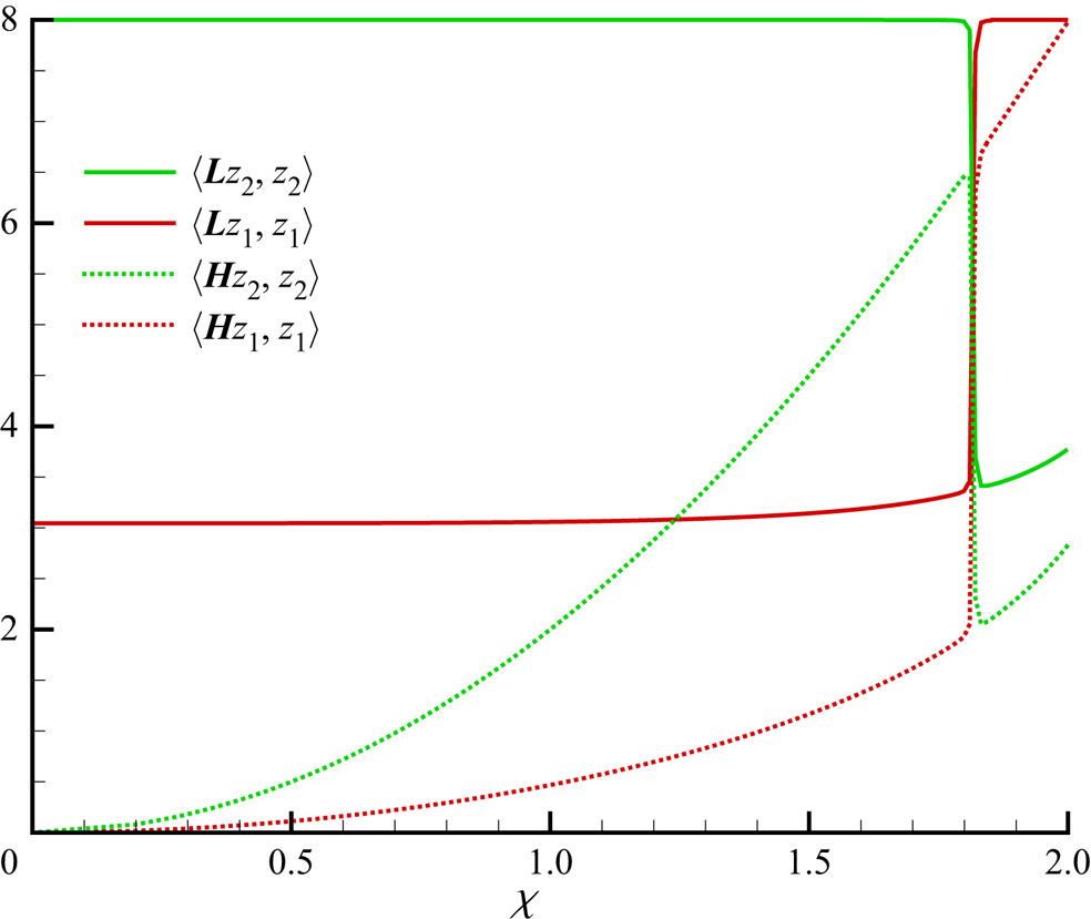
 $\langle \boldsymbol {H}z_i,z_i\rangle$ are the dimensionless kinetic, surface and electrostatic energies (recall (2.44)). Figure 7 shows the variation of the surface energy
 $\langle \boldsymbol {L}z_i,z_i\rangle$ and electrostatic energy
 $\langle \boldsymbol {H}z_i,z_i\rangle$ with dimensionless charge
 $\chi$ for the first and second modes of a charged drop constrained at
 $a=1/\sqrt {3}$. Figure 7 makes plain that for both modes of oscillation, the surface energy (area) of the RCCD is virtually constant when
 $\chi < 1.82$ albeit with the surface energy of the second mode being larger than that of the first. Over the same range of charge, figure 7 shows that the electrostatic energy of a RCCD is not only larger but increases much more rapidly with dimensionless charge for the second mode than the first. Given that
 $\lambda _i \approx \langle \boldsymbol {L}z_i,z_i\rangle - \langle \boldsymbol {H}z_i,z_i\rangle$, this increased variation in electrostatic energy for the second mode and the near constancy of surface energies for both modes clearly indicates that
 $\lambda _2$ and
 $\lambda _1$ must approach each other as
 $\chi$ increases. More importantly, figure 7 clearly shows that when
 $\chi >1.82$, the relative magnitudes of the surface and electrostatic energies for the two modes have switched: when
 $\chi > 1.82$, the first mode has adopted the characteristics of the second mode and vice versa compared with the situation when
 $\chi < 1.82$. In other words, when
 $\chi > 1.82$, the surface and electrostatic energies of the first mode are larger than those of the second mode. This exchange has important implications for the stability of a constrained drop near the Rayleigh charge limit (
 $\chi =2$) for mode 2.
Variation of the squares of the first eigenfrequency ( $\lambda _1$), the second eigenfrequency (
 $\lambda _2$) and the Rayleigh frequency (
 $\varOmega ^2_2$) with dimensionless charge (
 $\chi$) for a charged drop constrained at
 $a = 1/\sqrt {3}$.

Variation of the surface energy  $\langle \boldsymbol {L}z_i,z_i\rangle$ (solid curves) and the electrostatic energy
 $\langle \boldsymbol {H}z_i,z_i\rangle$ (dotted curves) for the first (
 $i=1$, red) and second (
 $i=2$, green) modes of oscillations with dimensionless charge (
 $\chi$) for a charged drop constrained at
 $a = 1/\sqrt {3}$.

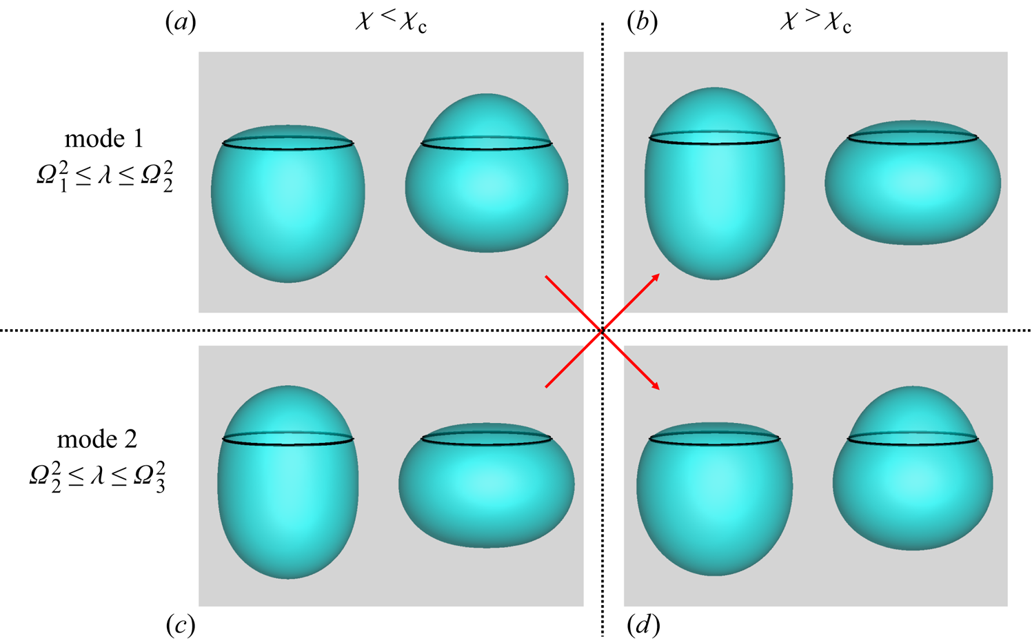
The implications in the exchange of modal behaviour observed here are best appreciated by considering the behaviour of two charged drops, one free and the other constrained at the natural pinning location for the second mode of oscillation ( $a=1/\sqrt {3}$).
(a) For values of charge less than
 $\chi =1.82$, the second mode of oscillation for these two drops, as discussed in § 4.1, is identical: the constraint has no effect whatsoever on the dynamics and both drops oscillate between prolate and oblate spheroidal shapes with no COM motion. While the first mode of oscillation does not exist for the free drop, the dynamics of this mode for the constrained drop is unique with respect to and distinct from all the other modes. Specifically, the unique signature of the dynamics of this mode of oscillation is characterized by axial translation of the COM. This oscillatory motion occurs with a distinct frequency which is, moreover, lower than the frequency of the second mode (figure 8).
(b) When
$\chi > 1.82$, these characteristics flip (figure 8) such that the prolate–oblate oscillation of the charged constrained drop can now be identified as the first (or fundamental) mode of oscillation because it is the mode that exhibits the lowest vibration frequency and, moreover, it is identical to the second mode of oscillation of a free charged drop. Furthermore, above this particular value of $\chi$, the second mode of oscillation for the constrained charged drop is characterized by COM translation. As dimensionless charge $\chi \to 2$, the mode that is characterized by prolate–oblate oscillations for both the constrained and free drops becomes unstable (mode 1 for the former but mode 2 for the latter), but the mode that entails COM translation (mode 2 for the RCCD drop) retains its stability.


Three-dimensional renderings of shapes of RCCDs that are constrained at  $a = 1/\sqrt {3}$ which are undergoing first (a,b) and second (c,d) mode oscillations. In panels (a,c), the dimensionless charge
 $\chi$ is less than the critical charge
 $\chi _c = 1.82$, i.e.
 $\chi < \chi _c$; in panels (b,d),
 $\chi > \chi _c$. In panels (a,c) where
 $\chi <1.82$, mode 1, panel (a), which involves COM motion, occurs at a lower frequency than mode 2, panel (b), which entails prolate–oblate oscillations. When
 $\chi >1.82$, the characteristics of these modes of oscillation, as indicated by the red arrows, exchange: the mode involving prolate–oblate oscillations, panel (b), now occurs at a lower frequency than the mode that involves oscillations of the COM, panel (d). In panels (a,c),
 $\chi =1.810175$,
 $\varOmega _1^2=0$,
 $\varOmega _2^2 = 1.446533$. In panels (b,d),
 $\chi =1.832114$,
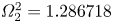 $\varOmega _2^2 = 1.286718$,
 $\varOmega _3^2=9.860154$. In panel (a),
 $\lambda _1 = 1.415551$,
 $\varLambda _1 = 0.978583$; in panel (c)
 $\lambda _2 = 1.446657$,
 $\varLambda _2 = 1.000014$; in panel (b)
 $\lambda _1 = 1.286608$,
 $\varLambda _1 = 0.999913$; in panel (d)
 $\lambda _2=1.391819$,
 $\varLambda _2=1.012259$.

5. Conclusions and outlook
The results presented in this paper have in large part been made possible thanks to work that began almost a century and a half earlier, and three pioneering papers. In the first of these, a landmark paper that is key to understanding virtually all subsequent work on interface oscillations, Rayleigh (Reference Rayleigh1879) showed that a free spherical drop of an incompressible, inviscid liquid subjected to small-amplitude perturbations undergoes stable linear oscillations. In particular, Rayleigh showed that there exist a countably infinite number of linear modes of oscillation,  $n=2, 3, \ldots$, each of which has a characteristic frequency and mode shape. Of no less importance was a follow-up paper by Rayleigh (Reference Rayleigh1882) in which he showed that if the drop is highly conducting and is surrounded by a highly insulating outer fluid (e.g. a drop of a liquid metal or even of water and salt that is surrounded by air), adding charge to the drop lowers the frequency of each mode and can lead to instability if the amount of charge exceeds a critical value. This limit is now known as the Rayleigh limit and has implications in a myriad of fields outside of the subject of the present paper including electrohydrodynamic tip streaming (Collins et al. Reference Collins, Jones, Harris and Basaran2008, Reference Collins, Sambath, Harris and Basaran2013) and electrosprays (Fernández de La Mora Reference Fernández de La Mora2007). A particular outcome of these two papers, which has important ramifications for the present work, is that for both uncharged and charged free drops, the
 $n=0$ and
 $n=1$ modes are disallowed because the first would result in violation of volume (mass) conservation and the second would result in the motion of the drop's COM. Also of interest to the present paper is that while Rayleigh (Reference Rayleigh1882) showed that all modes (
 $n \ge 2$) can be destabilized by a sufficient amount of charge, the first mode to become unstable is the
 $n=2$ prolate–oblate mode. A singularly important result from Rayleigh's two pioneering works, and one that stands in direct contrast to those of the present paper, is that for both uncharged and charged free drops, there is a one-to-one correspondence between mode number and mode shape (each mode shape in Rayleigh's works is given by a Legendre polynomial). The third leg, which is equally important as the other two by Rayleigh in making possible the present paper, entailed the study by Bostwick & Steen (Reference Bostwick and Steen2009) of oscillations of spherical drops that are not free but instead are constrained by or pinned on an infinitesimally thin solid ring or circle of contact. A key consequence of pinning is to introduce a new low-frequency mode of oscillation (
 $n=1$). The new mode is associated primarily with COM translation of the constrained drop. With these three foundational papers, it then became possible to analyse theoretically in the present paper the effect of charge on the linear oscillations of a constrained drop.
By using normal mode analysis and methods for solving linear operator eigenvalue problems, we have obtained an implicit expression for the frequency (square root of the eigenvalue) of each mode of oscillation. According to the foregoing results, for RCCDs, the association between mode number and mode shape can be lost. Free drops exhibit the physically simple and easy to visualize oscillatory response such that if one were to look at (one half of) the cross-sectional profile of a drop, the number of times the interface intersects the cross-section of the original sphere identically equals the mode number during linear oscillations, e.g. there are two crossings for the  $n=2$ mode and five crossings for the
 $n=5$ mode. By contrast, during oscillations of RCCDs, the different modes are identified and ordered by their frequencies, i.e. the lowest mode is that with the lowest frequency, the next mode is that with the second lowest frequency, and so on. Moreover, we have shown in this paper that for certain pinning locations, the dynamics exhibits the phenomenon of eigenvalue veering as drop charge increases. For example, while a RCCD that is pinned at the zero of the second Legendre polynomial has a first mode that involves COM motion and a second mode that involves prolate–oblate oscillations when drop charge is non-zero but small, the modes flip when drop charge exceeds a critical value. Thereafter, the prolate–oblate oscillation of the RCCD can now be identified as the first (or fundamental) mode of oscillation because it is the mode that exhibits the lowest vibration frequency. Here, we have determined the value of (dimensionless) charge for which the characteristics of the modes flip to be
 $\chi \approx 1.82$. At the Rayleigh limit, it is the first eigenmode involving prolate–oblate oscillations that loses stability while the second eigenmode involving COM motion remains stable.
Many obvious but important extensions of the analysis presented in this paper on linear oscillations of RCCDs are not only possible but warranted. Some conceptually straightforward extensions include accounting for the constrained charged drop's viscosity (cf. Bostwick & Steen Reference Bostwick and Steen2013b), the presence of a viscous outer fluid (cf. Miller & Scriven Reference Miller and Scriven1968) and surfactants with and without surface rheological effects (Lopez & Hirsa Reference Lopez and Hirsa2000; Vlahovska, Blawzdziewicz & Loewenberg Reference Vlahovska, Blawzdziewicz and Loewenberg2009; Wee et al. Reference Wee, Wagoner, Kamat and Basaran2020, Reference Wee, Wagoner, Garg, Kamat and Basaran2021). Some other possible extensions include studying oscillations of uncharged constrained drops driven by an externally imposed electric field and also oscillations under the combined influence of both drop charge and an externally applied electric field. However, less obvious but scientifically and practically important extensions of this work are not only possible but highly desirable.
The less obvious but potentially useful extensions hold the promise for designing new grab-and-release applications (Bostwick & Steen Reference Bostwick and Steen2009), adaptive liquid lenses (Hirsa et al. Reference Hirsa, López, Laytin, Vogel and Steen2005) and adaptive valves that can for example block or unblock the flow in a conduit. These extensions are all based on exploiting the equilibria and stability of DDSs in the absence (Hirsa et al. Reference Hirsa, López, Laytin, Vogel and Steen2005) and presence of electric fields (Sambath & Basaran Reference Sambath and Basaran2014). The equilibrium shape of a DDS consists of two identical subhemispherical drops when the combined volume of the two drops is smaller than that of a sphere of the same radius as the hole in the associated solid substrate (figure 1). When the combined volume of the top and bottom drops, however, exceeds that of the sphere, the shape that corresponds to two equal superhemispherical drops is an unstable equilibrium state (Hirsa et al. Reference Hirsa, López, Laytin, Vogel and Steen2005). For these larger volume DDSs, the two stable states correspond to two drops of unequal volumes but identical radii of curvature such that the two drops are the result of cutting unequally a sphere that is larger than a sphere of the same radius as the hole in the solid plate (Hirsa et al. Reference Hirsa, López, Laytin, Vogel and Steen2005). Many applications of DDSs are based on toggling the system between the state where the top drop is large and the bottom drop is small and that where the top drop is small and the bottom drop is large. Sambath & Basaran (Reference Sambath and Basaran2014) have theoretically analysed the equilibrium states and stability of electrified DDSs and how electric fields can be used to toggle the system between its equilibrium states. The latter work can be extended by coupling net charge on the drops with an applied electric field for improved control. In a real application, the droplets are likely to undergo oscillations during toggling. Clearly, analyses of both linear and nonlinear oscillations of electrified DDSs will be needed before such applications can be fully realized in practical situations.
Acknowledgements
O.A.B. also thanks (the late) Professor P. Steen of Cornell and Professor A. Hirsa of RPI for exposing him early on to the exciting subject of capillary switches.
Funding
The authors thank the Purdue Process Safety and Assurance Center (P2SAC), the Gedge Professorship to O.A.B. and the Bilsland Dissertation Fellowship to B.W.W. for financial support.
Declaration of interests
The authors report no conflict of interest.
Appendix A. Consequence of the uniformity of the electric potential along the free surface
In this short appendix, we provide two different derivations of (2.30). In the first derivation, we exploit the fact that the electric potential on the surface of a conductor is spatially uniform but not necessarily temporally constant,
 \begin{equation} V|_{r=f}= (V_0 + V')|_{r=f} = \mathcal{F}(t), \end{equation}
where  $\mathcal {F}(t)$ is a function of time. Substitution of the expression for the base state potential
 $V_0$ in (A1) and linearization then leads to
 \begin{equation} \frac{-Q}{4{\rm \pi}\epsilon_e R^2}\eta + V'|_{r=R} = \mathcal{F}(t) - \frac{Q}{4{\rm \pi}\epsilon_e R}. \end{equation}
It is clear from the previous equation that the left-hand side depends both on cone angle ( $\theta$) and time (
 $t$) while the right-hand side is independent of
 $\theta$. Therefore, differentiating equation (A2) with respect to
 $\theta$ and writing the perturbations using their normal mode expressions ((2.21)–(2.24)) directly leads to (2.30).
The requirement that the surface of a conductor is equipotential (spatially constant) is identical to requiring that the tangential component of the electric field at the surface of the conductor vanishes (see (2.13)). Using the expressions for the unit tangent and the gradient in spherical coordinates, (2.13) can be written as
 \begin{equation} \left.(\,f^2 + f^2_\theta)^{{-}1/2}\left[f_\theta\frac{\partial}{\partial r} (V_0 + V')+f\frac{1}{r}\frac{\partial}{\partial \theta} (V_0+V')\right] \right|_{r=f}=0. \end{equation}
Evaluation and linearization of (A3) yields, at leading order, the following expression:
 \begin{equation} V'_{\theta}|_{r=R}-\frac{Q}{4{\rm \pi}\epsilon_e R^2}\eta_\theta=0. \end{equation}
The previous expression is identically the  $\theta$ derivative of (A2) and plainly leads to (2.30) when the perturbations are once again represented in terms of their normal mode expressions ((2.21)–(2.24)).
Appendix B. Discussion on the various methods for constructing solutions to eigenvalue problems and handling of the pinning ring
As has been discussed by Bostwick & Steen (Reference Bostwick and Steen2013a), different methods for solving (2.39) or its analogues can be thought of as using different function spaces or bases. In the pioneering work of Bostwick & Steen (Reference Bostwick and Steen2009), the approach that is used restricted the analysis to smooth interfaces such that the derivative of the shape function, or equivalently the contact angle, was continuous across the circle of contact or ring constraint. Bostwick & Steen (Reference Bostwick and Steen2013a) refer to such solutions as B09 continuous solutions. However, experiments carried out with DDSs or CSs (figure 1) show that the contact angle that the top and the bottom droplets make with the solid substrate can be discontinuous (Theisen et al. Reference Theisen, Vogel, Lopez, Hirsa and Steen2007; Bostwick & Steen Reference Bostwick and Steen2009). In the formulation adopted later by Bostwick & Steen (Reference Bostwick and Steen2013a) where the solutions are referred to EX, the shape function can have a discontinuous derivative at the circle of contact. At approximately the same time, two different groups have reported different approaches to analysing this problem.
Prosperetti (Reference Prosperetti2012) has solved the pinned circle-of-contact problem using expansions of the free surface and velocity potential in terms of spherical harmonics. In his approach, the singularity in the curvature must be explicitly accounted for in situations where the derivative is not continuous. It has been shown by Bostwick & Steen (Reference Bostwick and Steen2013a) that Prosperetti's frequencies are in excellent agreement with the EX frequencies.
Ramalingam et al. (Reference Ramalingam, Ramkrishna and Basaran2012) have used two different approaches to determine the frequencies of oscillations of RCDs. In the main approach that is used in their paper, they recast the eigenvalue problem into a Rayleigh–Ritz type minimization problem and seamlessly incorporate the fixed point constraint into the analysis by means of a Lagrange multiplier. Bostwick & Steen (Reference Bostwick and Steen2013a) refer to this approach as ‘their EX’ (see below). In the second approach, Ramalingam et al. (Reference Ramalingam, Ramkrishna and Basaran2012) have employed a method based on a composite Green's function such that the composite function consists of two non-zero Green's functions, one for each free surface, i.e. the free surface above and the free surface below the contact point. In referring to Ramalingam et al. (Reference Ramalingam, Ramkrishna and Basaran2012), Bostwick & Steen (Reference Bostwick and Steen2013a) have written the following on pages 333 and 334 of their paper and which we quote verbatim: ‘Ramalingam et al. (Reference Ramalingam, Ramkrishna and Basaran2012), which first came to the authors attention while Parts 1 and 2 were under final review, redoes the B09 problem allowing for non-smooth surfaces at pin locations. Their figure 8 compares B09 with their EX and further confirms our figure 2(a,b)’. A few points are worth noting regarding the work of Ramalingam et al. (Reference Ramalingam, Ramkrishna and Basaran2012). First, while Prosperetti (Reference Prosperetti2012) explicitly accounts for the curvature singularity using a delta function with an unknown coefficient and Ramalingam et al. (Reference Ramalingam, Ramkrishna and Basaran2012) introduces a Lagrange multiplier within a minimization formulation, the two techniques in the end produce the same expression for the free surface perturbation. By comparing (3.6) and (3.4) in this paper (and the corresponding equations in the paper by Ramalingam et al. (Reference Ramalingam, Ramkrishna and Basaran2012)) with the second term in (27) of Prosperetti (Reference Prosperetti2012), it is easily seen that the Lagrange multiplier here (and in Ramalingam et al. (Reference Ramalingam, Ramkrishna and Basaran2012)) and the coefficient of the delta singularity in Prosperetti (Reference Prosperetti2012) play identical roles. Second, as the number of polynomials in the expansions used to represent the shape and velocity potential are increased, the frequency obtained with the minimization method approaches that obtained with Green's method.