


1. Introduction
1.1. Motivation
Let us first recall the classical Sobolev inequality. For  $N\geq 3$, there exists
 $\mathcal{S}=\mathcal{S}(N) \gt 0$ such that
 \begin{equation}
\|\nabla u\|^2_{L^2(\mathbb{R}^N)}\geq \mathcal{S}\|u\|^2_{L^{2^*}(\mathbb{R}^N)},\quad \mbox{for all}\ u\in \mathcal{D}^{1,2}_0(\mathbb{R}^N),
\end{equation}
where  $2^*=2N/(N-2)$ and
 $\mathcal{D}^{1,2}_0(\mathbb{R}^N)$ is the closure of
 $C^\infty_c(\mathbb{R}^N)$ with respect to the norm
 $\|u\|_{\mathcal{D}^{1,2}_0(\mathbb{R}^N)}=\|\nabla u\|_{L^2(\mathbb{R}^N)}$. By employing rearrangement methods, Talenti [Reference Talenti23] determined the optimal constant and the extremal functions for inequality (1.1). In fact, equality in (1.1) is attained by the functions
 $cV_{\lambda,z}$ for all
 $c\in\mathbb{R}$, λ > 0 and
 $z\in\mathbb{R}^N$, where
 \begin{equation*}
V_{\lambda,z}(x)=[N(N-2)]^{\frac{N-2}{4}}\lambda^{\frac{N-2}{2}}
\left(1+\lambda^2|x-z|^2\right)^{-\frac{N-2}{2}}
\end{equation*}
is the unique (up to scalings and translations) nontrivial nonnegative solution of the related Euler–Lagrange equation
 \begin{equation*}
-\Delta u=|u|^{2^*-2}u\quad \mbox{in}\ \mathbb{R}^N.
\end{equation*}
For details, see [Reference Caffarelli, Gidas and Spruck5]. Brezis and Lieb [Reference Brézis and Lieb4] posed the famous question of whether a remainder term, proportional to the quadratic distance of the function to the manifold  $\mathcal{M}:=\{cV_{\lambda,z}: c\in\mathbb{R}, \lambda \gt 0, z\in\mathbb{R}^N\}$, Bianchi and Egnell [Reference Bianchi and Egnell2] answered this question affirmatively, demonstrating that there exists a constant
 $c_{\mathrm{BE}} \gt 0$ such that
 \begin{equation}
\|\nabla u\|^2_{L^2(\mathbb{R}^N)}
-\mathcal{S}\|u\|^2_{L^{2^*}(\mathbb{R}^N)}
\geq c_{\mathrm{BE}} \mathrm{dist}(u,\mathcal{M})^2,\quad \mbox{for all}\ u\in \mathcal{D}^{1,2}_0(\mathbb{R}^N).
\end{equation}
where  $\mathrm{dist}(u,\mathcal{M}):=\inf_{v\in \mathcal{M}}\|\nabla (u-v)\|_{L^2(\mathbb{R}^N)}$. Subsequently, this result was extended to the second-order case [Reference Lu and Wei22], and the case of arbitrary higher order [Reference Bartsch, Weth and Willem1]. Chen et al. [Reference Chen, Frank and Weth10] established the stability of the Sobolev inequality in the general fractional space
 $\mathcal{D}^{s,2}_0(\mathbb{R}^N)$ with
 $s\in (0,N/2)$, i.e.,
 \begin{equation*}
\|(-\Delta)^{s/2} u\|^2_{L^2(\mathbb{R}^N)}
-\mathcal{S}_s\|u\|^2_{L^{2^*_s}(\mathbb{R}^N)}
\geq c_{\mathrm{BE}}(s) \mathrm{dist}(u,\mathcal{M}_s)^2,\quad \mbox{for all}\ u\in \mathcal{D}^{s,2}_0(\mathbb{R}^N),
\end{equation*}
where  $2^*_s=2N/(N-2s)$ and
 $\mathcal{M}_s=\{c\lambda^{(N-2s)/2}V_s(\lambda(x-z)): c\in\mathbb{R}, \lambda \gt 0, z\in\mathbb{R}^N\}$ with
 $V_s(x)=(1+|x|^2)^{(2s-N)/2}$, and
 $\mathrm{dist}(u,\mathcal{M}_s):=
\inf_{v\in \mathcal{M}_s}\|(-\Delta)^{s/2} (u-v)\|_{L^2(\mathbb{R}^N)}$. Moreover, the behaviour near the extremal functions set
 $\mathcal{M}_s$ as shown in [Reference Chen, Frank and Weth10, Proposition 2], i.e., for all
 $u\in \mathcal{D}^{s,2}_0(\mathbb{R}^N)$ with
 $\mathrm{dist}(u,\mathcal{M}_s) \lt \|(-\Delta)^{s/2}u\|_{L^2(\mathbb{R}^N)}$,
 \begin{align}
\mathrm{dist}(u,\mathcal{M}_s)^2
& \geq \|(-\Delta)^{s/2} u\|^2_{L^2(\mathbb{R}^N)}
-\mathcal{S}_s\|u\|^2_{L^{2^*_s}(\mathbb{R}^N)}
\nonumber \\
& \geq \frac{4s}{N+2+2s}\mathrm{dist}(u,\mathcal{M}_s)^2
+o\left(\mathrm{dist}(u,\mathcal{M}_s)^2\right),
\end{align}
implies that
 \begin{align*}
c_{\mathrm{BE}}(s)\leq \frac{4s}{N+2+2s},\quad \mbox{for all}\ N\geq 1.
\end{align*}
We refer to the recent works [Reference Chen, Lu and Tang8, Reference Chen, Lu and Tang9, Reference Dolbeault, Esteban, Figalli, Frank and Loss13] regarding the explicit lower bound of  $c_{\mathrm{BE}}(s)$. Now, let us mention the minimizing problem
 \begin{equation*}
c_{\mathrm{BE}}(s) =\inf_{u\in \mathcal{D}^{s,2}_0(\mathbb{R}^N)\setminus \mathcal{M}_s}\Phi(u),
\end{equation*}
where
 \begin{equation*}
\Phi(u)=\frac{\|(-\Delta)^{s/2} u\|^2_{L^2(\mathbb{R}^N)}
-\mathcal{S}_s\|u\|^2_{L^{2^*_s}(\mathbb{R}^N)}}{\inf_{v\in \mathcal{M}_s}\|(-\Delta)^{s/2} (u-v)\|^2_{L^2(\mathbb{R}^N)}}.
\end{equation*}
Recently, König [Reference König18] provided an upper bound with strict inequality  $c_{\mathrm{BE}}(s) \lt \frac{4s}{N+2+2s}$ for all
 $N\geq 2$, by taking the test function
 $V_s+\epsilon \rho_2$ with
 $0 \lt \epsilon\ll 1$, i.e.,
 \begin{align}
c_{\mathrm{BE}}(s)\leq \Phi(V_s+\epsilon \rho_2) \lt \frac{4s}{N+2+2s},\quad \mbox{for}\ \epsilon\ll 1.
\end{align}
Here ρ 2 is an extremal function of the following spectral gap inequality: let  $T_{V_s}\mathcal{M}_s$ be the tangent space of
 $\mathcal{M}_s$ at Vs, for all
 $\rho\in (T_{V_s}\mathcal{M}_s)^\bot$,
 \begin{align*}
&\|(-\Delta)^{s/2} u\|^2_{L^2(\mathbb{R}^N)}
-\mathcal{S}_s(2^*_s-1)\|V_s\|^{2-2^*_s}_{L^{2^*_s}(\mathbb{R}^N)}
\int_{\mathbb{R}^N}V_s^{2^*-2}\rho^2\mathrm{d}x\\
&\qquad\geq \frac{4s}{N+2+2s}\|(-\Delta)^{s/2}\rho\|^2_{L^2(\mathbb{R}^N)}.
\end{align*}
Furthermore, König [Reference König20] also proved that  $c_{\mathrm{BE}}(s) \lt 2-2^{\frac{2}{2^*_s}}$ for all
 $N\geq 1$ by taking the test function
 $u_\lambda(x)=V_s(x)+\lambda^{(N-2s)/2}V_s(\lambda x)$ with λ sufficiently small, i.e.,
 \begin{equation}
c_{\mathrm{BE}}(s)\leq \Phi(u_\lambda) \lt 2-2^{\frac{2}{2^*_s}},\quad \mbox{for}\ \lambda\ll 1.
\end{equation}
Combining the upper estimates (1.4) and (1.5), König [Reference König20] demonstrated an interesting phenomenon: there exists a minimizer of  $c_{\mathrm{BE}}(s)$ for all
 $N\geq 2$, by using a concentration-compactness type argument on the distance functional
 $\mathrm{dist}(u,\mathcal{M}_s)$. While for N = 1 and
 $s\in (0,1/2)$, König [Reference König19] showed that there exists a neighbourhood
 $\mathcal{N}\subset \mathcal{D}^{s,2}_0(\mathbb{R})$ of
 $\mathcal{M}_s$ such that, for all
 $u\in \mathcal{N}\setminus \mathcal{M}_s$,
 $\Phi(u)\geq \frac{4s}{3+2s}$, and the author conjectured that in this case
 $c_{\mathrm{BE}}(s)$ may not have a minimizers. The key step in proving the existence of minimizers for
 $c_{\mathrm{BE}}(s)$ appears to be showing the strict inequality
 $c_{\mathrm{BE}}(s) \lt 4s/(N+2+2s)$. See also [Reference Tang, Zhang and Zhang24] about the existence of minimizers of
 $c_{\mathrm{BE}}$ on the Heisenberg group.
Now, let us mention the famous Caffarelli–Kohn–Nirenberg (we write CKN for short) inequality which was first introduced by Caffarelli et al. in their seminal work [Reference Caffarelli, Kohn and Nirenberg6] in 1984. Here, we just focus on the case without interpolation term, i.e.,
 \begin{equation}
\mathcal{S}_{a,b}\left(\int_{\mathbb{R}^N}|x|^{-qb}|u|^q \mathrm{d}x\right)^{\frac{2}{q}}
\leq \int_{\mathbb{R}^N}|x|^{-2a}|\nabla u|^2 \mathrm{d}x, \quad \mbox{for all}\ u\in \mathcal{D}^{1,2}_a(\mathbb{R}^N),
\end{equation}
for some best constant  $\mathcal{S}_{a,b}:=\mathcal{S}(N,a,b) \gt 0$, where
 \begin{eqnarray*}
-\infty \lt a \lt a_c:=\frac{N-2}{2},\ q=\frac{2N}{N-2(1+a-b)}\ \mbox{and}\
\left\{\begin{array}{ll}
a\leq b\leq a+1,\ \mbox{if}\ N\geq 3;\\[3mm]
a \lt b\leq a+1,\ \mbox{if}\ N=2;\\[3mm]
a+\frac{1}{2} \lt b\leq a+1,\ \mbox{if}\ N=1,
\end{array}
\right.
\end{eqnarray*}
and  $\mathcal{D}^{1,2}_a(\mathbb{R}^N)$ is the closure of
 $C^\infty_c(\mathbb{R}^N)$ with respect to the inner product
 \begin{align*}
\langle u,v\rangle_{\mathcal{D}^{1,2}_a(\mathbb{R}^N)}
=\int_{\mathbb{R}^N}|x|^{-2a}\nabla u\cdot \nabla v\mathrm{d}x,
\end{align*}
and the norm  $\|u\|_{\mathcal{D}^{1,2}_a(\mathbb{R}^N)}=\langle u,u\rangle_{\mathcal{D}^{1,2}_a(\mathbb{R}^N)}^{1/2}$. When
 $N\geq 3$,
 $0\leq a \lt a_c$ and
 $a\leq b \lt a+1$, Chou and Chu [Reference Chou and Chu11] proved that the extremal functions are radially symmetric by using the moving planes method. When
 $b=a+1$ for all cases
 $N\geq 1$ or a < 0 and b = a for the case
 $N\geq 3$, Catrina and Wang [Reference Catrina and Wang7] proved that
 $\mathcal{S}_{a,b}$ is not achieved and for other cases it is always achieved. Moreover, the authors in [Reference Catrina and Wang7] also obtained the symmetry breaking result: for N = 1, no extremal functions are radial for all
 $a \lt -\frac{1}{2}$ and
 $a+\frac{1}{2} \lt b \lt a+1$, and for
 $N\geq 2$, there exists a function h(a) depending on a such that the extremal functions of
 $\mathcal{S}_{a,b}$ are nonradial if (a, b) satisfies a < 0 and
 $a \lt b \lt h(a)$. In [Reference Felli and Schneider16], Felli and Schneider obtained the explicit form of h(a) when
 $N\geq 3$, which is now known as the Felli–Schneider curve,
 \begin{equation*}
b_{\mathrm{FS}}(a):=\frac{N(a_c-a)}{2\sqrt{(a_c-a)^2+N-1}}
+a-a_c.
\end{equation*}
In fact, this also holds for the case N = 2 (see [Reference Dolbeault, Esteban and Tarantello15]), i.e., when a < 0 and  $a \lt b \lt b_{\mathrm{FS}}(a)$, the extremal functions of
 $\mathcal{S}_{a,b}$ are nonradial. Finally, in a remarkable paper, Dolbeault et al. [Reference Dolbeault, Esteban and Loss14] obtained the optimal rigidity result by using the so-called carré du champ method: when a < 0 and
 $b_{\mathrm{FS}}(a)\leq b \lt a+1$ for all
 $N\geq 2$, the extremal functions are radially symmetric. Now, in the symmetric region (hereafter we always assume
 $|a|+|b|\neq 0$):
 \begin{align}
& N=2,\ \left\{(a,b): b_{\mathrm{FS}}(a)\leq b \lt a+1, a \lt 0\right\};
\nonumber\\
& N\geq 3,\ \left\{(a,b): b_{\mathrm{FS}}(a)\leq b \lt a+1, a \lt 0\right\}
\cup \left\{(a,b): a\leq b \lt a+1, 0\leq a \lt a_c\right\},
\end{align}
let us denote
 \begin{align}
\mathcal{M}_{a,b}=\left\{cU_\lambda: c\in\mathbb{R}, \lambda \gt 0\right\}
\end{align}
as the set of extremal functions of the CKN inequality (1.6). Here,  $U_\lambda(x)=\lambda^{a_c-a}U(\lambda x)$,
 \begin{equation}
U(x)=D_{a,b}\left(1+|x|^{(a_c-a)(q-2)}\right)
^{-\frac{2}{q-2}},
\end{equation}
with
 \begin{equation}
D_{a,b}=\left[\tau^{2}K(K-2)\right]^{\frac{K-2}{4}},\ \tau=\frac{(a_c-a)(1+a-b)}{a_c-a+b},\ K=\frac{N}{1+a-b},
\end{equation}
such that Uλ is the unique (up to scalings) nontrivial nonnegative solution (see [Reference Dolbeault, Esteban and Loss14]) of the related Euler–Lagrange problem
 \begin{equation}
-\mathrm{div}(|x|^{-2a}\nabla u)=|x|^{-bq} |u|^{q-2}u \quad\mbox{in}\ \mathbb{R}^N,\quad \int_{\mathbb{R}^N}|x|^{-bq}|u|^q\mathrm{d}x \lt \infty.
\end{equation}
As mentioned previously, once the extremal functions of (1.6) are well understood, it is natural to investigate the quantitative stability of the CKN inequality (1.6) by asking whether the deviation of a given function from attaining equality in (1.6) controls its distance from the family of extremal functions. Successfully, Wei and Wu [Reference Wei and Wu25] established the stability result when  $N\geq 3$ and (1.7) holds except for
 $b=b_{\mathrm{FS}}(a)$, which states that for all
 $u\in \mathcal{D}^{1,2}_a(\mathbb{R}^N)$,
 \begin{align}
\int_{\mathbb{R}^N}|x|^{-2a}|\nabla u|^2 \mathrm{d}x
-\mathcal{S}_{a,b}\left(\int_{\mathbb{R}^N}|x|^{-qb}|u|^q \mathrm{d}x\right)^{\frac{2}{q}}
\geq c_{a,b}
\mathrm{dist}(u,\mathcal{M}_{a,b})^2,
\end{align}
where
 \begin{equation*}
\mathrm{dist}(u,\mathcal{M}_{a,b})=\left(\inf_{v\in \mathcal{M}_{a,b}}\int_{\mathbb{R}^N}|x|^{-2a}|\nabla (u-v)|^2 \mathrm{d}x\right)^{1/2}.
\end{equation*}
As shown in the previous preprint [Reference Deng and Tian12] (see also [Reference Wei and Wu26]), such stability result (1.12) also holds for N = 2. When  $b=b_{\mathrm{FS}}(a)$ and a < 0, (1.6) allows remainder term with order four of the distance functional proved by Frank and Peteranderl [Reference Frank and Peteranderl17], i.e., there exists a constant
 $c_{a} \gt 0$ such that for all
 $u\in\mathcal{D}^{1,2}_a(\mathbb{R}^N)\setminus\{0\}$,
 \begin{align*}
&\int_{\mathbb{R}^N}|x|^{-2a}|\nabla u|^2 \mathrm{d}x
-\mathcal{S}_{a,b}\left(\int_{\mathbb{R}^N}|x|^{-qb}|u|^q \mathrm{d}x\right)^{\frac{2}{q}}\\
&\qquad\geq c_{a}
\mathrm{dist}(u,\mathcal{M}_{a,b})^4
\left(\int_{\mathbb{R}^N}|x|^{-2a}|\nabla u|^2 \mathrm{d}x\right)^{-1},
\end{align*}
moreover, the inequality is best possible with respect to the power four.
Then, when (1.7) holds except for  $b=b_{\mathrm{FS}}(a)$, it is natural to consider the following minimization problem
 \begin{align}
c_{a,b}:
=\inf_{u\in \mathcal{D}^{1,2}_{a}(\mathbb{R}^N)
\setminus \mathcal{M}_{a,b}}
\mathcal{E}(u) \gt 0,
\end{align}
where
 \begin{align}
\mathcal{E}(u):=\frac{\int_{\mathbb{R}^N}|x|^{-2a}|\nabla u|^2 \mathrm{d}x
-\mathcal{S}_{a,b}\left(\int_{\mathbb{R}^N}|x|^{-qb}|u|^q \mathrm{d}x\right)^{\frac{2}{q}}}
{\mathrm{dist}(u,\mathcal{M}_{a,b})^2},\quad u\in \mathcal{D}^{1,2}_{a}(\mathbb{R}^N)
\setminus \mathcal{M}_{a,b}.
\end{align}
Recently, Wei and Wu [Reference Wei and Wu26] proved that  $c_{a,b}$ has a minimizer if
 \begin{align}
& N=2,\ a \lt 0\ \mbox{and}\ b_{\mathrm{FS}}^*(a)\leq b \lt a+1;
\nonumber\\
& N\geq 3,\ \mbox{either}\ a_c^* \lt a \lt a_c\ \mbox{and}\ a\leq b \lt a+1,
\ \mbox{or}\ a\leq a_c^*\ \mbox{and}\ b_{\mathrm{FS}}^*(a)\leq b \lt a+1,
\end{align}
where
 \begin{align}
a_c^*=\left(1-\sqrt{\frac{N-1}{2N}}\right)a_c,
\quad b^*_{\mathrm{FS}}(a)=\frac{(a_c-a)N}{a_c-a+\sqrt{(a_c-a)^2+N-1}}+a-a_c.
\end{align}
It is obvious that  $b^*_{\mathrm{FS}}(a) \gt b_{\mathrm{FS}}(a)$ for all
 $a \lt a_c$, thus the region of (a, b) in (1.15) is slightly smaller than (1.7). In fact, if (1.7) holds, the authors in [Reference Wei and Wu26] obtained the crucial spectral gap inequality: let
 $T_U\mathcal{M}_{a,b}$ be the tangent space of
 $\mathcal{M}_{a,b}$ at U, then for all
 $\phi\in (T_U\mathcal{M}_{a,b})^\bot$,
 \begin{align}
\int_{\mathbb{R}^N}|x|^{-2a}|\nabla \phi|^2 \mathrm{d}x
-(q-1)\int_{\mathbb{R}^N}|x|^{-qb}U^{q-2}\phi^2 \mathrm{d}x
\geq \Lambda_*\int_{\mathbb{R}^N}|x|^{-2a}|\nabla \phi|^2 \mathrm{d}x,
\end{align}
where
 \begin{eqnarray}
\Lambda_*=\Lambda_*(a,b)=
\left\{\begin{array}{ll}
\Lambda_1(a,b),\ \ &\mbox{if}\ (1.15)\ \mbox{holds},\\[2mm]
\Lambda_2(a,b),\ \ &\mbox{the remaining case}.
\end{array}
\right.
\end{eqnarray}
Here
 \begin{align*}
\Lambda_1(a,b)=\frac{2(q-2)}{3q-4},
\end{align*}
and
 \begin{align*}
&\Lambda_2(a,b)\nonumber \\
&\qquad=\frac{\sqrt{(a_c-a)^2+N-1}\left[\sqrt{(a_c-a)^2+N-1}
+\frac{(q-2)(a_c-a)}{2}\right]
-\frac{q(q-1)(a_c-a)^2}{2}}
{\sqrt{(a_c-a)^2+N-1}\left[\sqrt{(a_c-a)^2+N-1}+\frac{(q-2)(a_c-a)}{2}
\right]}.
\end{align*}
Note that  $q=\frac{2N}{N-2(a+1-b)} \gt 2$ and
 $a \lt a_c$, thus
 $\Lambda_1(a,b)$ is continuous about (a, b) in (1.15). Note also that
 $\Lambda_2(a,b)$ is a composite form of elementary functions, so it is also continuous about (a, b) in the remaining case. Moreover, from [Reference Wei and Wu26, Proposition 3.1], we know that when
 $b=b^*_{\mathrm{FS}}(a)$, for all
 $a \lt a_c^*$,
 \begin{align*}
\Lambda_1(a,b)=\Lambda_2(a,b).
\end{align*}
Therefore,  $\Lambda_*=\Lambda_*(a,b)$ is continuous about (a, b) in (1.7). Furthermore, if (a, b) is in the remaining region (that is,
 $a \lt a_c^*$ and
 $b_{\mathrm{FS}}(a) \lt b \lt b^*_{\mathrm{FS}}(a)$), then
 \begin{align*}
\Lambda_1(a,b) \gt \Lambda_2(a,b).
\end{align*}
By inequality (1.17), using the same arguments in [Reference Chen, Frank and Weth10, Proposition 2], it is not difficult to deduce the behaviour of  $\mathcal{E}$ near
 $\mathcal{M}_{a,b}$,
 \begin{align}
\liminf_{n\to\infty}\mathcal{E}(u_n)\geq \Lambda_*
\end{align}
for every sequence un that converges (in  $\mathcal{D}^{1,2}_{a}(\mathbb{R}^N)$) to
 $\mathcal{M}_{a,b}$, and
 $c_{a,b}\leq \Lambda_*$. The crucial step of proving the existence of minimizers of
 $c_{a,b}$ shows that
 \begin{align}
c_{a,b} \lt \Lambda_*,
\end{align}
which excludes the minimizing sequence of  $c_{a,b}$ tends to
 $\mathcal{M}_{a,b}$. The authors in [Reference Wei and Wu26, Proposition 4.1] proved that, if (1.15) holds, then
 $\mathcal{E}(U+\epsilon \phi_2^{(1)}) \lt \Lambda_*$ for
 $\epsilon\ll 1$, where
 $\phi_2^{(1)}$ is an extremal function of inequality (1.17) with explicit form, thus (1.20) holds. While for the remaining case, as shown in [Reference Wei and Wu26, Appendix A], it is difficult to show (1.20) even if taking quadruple Taylor expansion of
 $\mathcal{E}(U+\epsilon \phi_2^{(2)})$ for ϵ sufficiently small, where
 $\phi_2^{(2)}$ is an extremal function of (1.17) with explicit form in the remaining case.
Now, we focus on the remaining case about the existence of minimizers of  $c_{a,b}$.
1.2. Main results
As stated previously, when (1.15) holds, Wei and Wu [Reference Wei and Wu26] have proved the strict spectral inequality (1.20), then by using this result, the authors proved the existence of minimizers of  $c_{a,b}$. In the present paper, we will show (1.20) also holds near the curve
 $b=b_{\mathrm{FS}}^*(a)$ in a wider region of parameter (a, b) than (1.15) and prove the existence of minimizers of
 $c_{a,b}$.
Define a constant
 \begin{align}
a^*:=\frac{2(N-2)K^*-(K^*-2)\sqrt{2(N-1)K^*}}{4K^*},
\end{align}
where  $K^*\approx 6.698818$ is the unique solution of
 \begin{align}
2-2^{\frac{t-2}{t}}=\frac{4}{t+4},\quad \mbox{for}\ t \gt 2,
\end{align}
see lemma A.1 for details. Now, we state the following attainability result.
Theorem 1.1. For each  $a \lt \min\{a_c^*,a^*\}$, there is
 $\epsilon_{N,a}\in (0, b^*_{\mathrm{FS}}(a)-b_{\mathrm{FS}}(a))$ depending only on N and a such that, the strict inequality (1.20) holds for
 $b\in [b^*_{\mathrm{FS}}(a)-\epsilon_{N,a},b^*_{\mathrm{FS}}(a))$. Moreover, in this case,
 $c_{a,b}$ can also be achieved, i.e., there is
 $u_0\in \mathcal{D}^{1,2}_{a}(\mathbb{R}^N)
\setminus \mathcal{M}_{a,b}$ such that
 $\mathcal{E}(u_0)=c_{a,b}$.
Moreover, following the work of Chen et al. [Reference Chen, Frank and Weth10, Proposition 2] shown as in (1.3), we give the upper bound of CKN inequality in the symmetry region (1.7), which may have its own interests.
Theorem 1.2. Assume that (1.7) holds. For all  $u\in \mathcal{D}^{1,2}_a(\mathbb{R}^N)$,
 \begin{align}
1\cdot \mathrm{dist}(u,\mathcal{M}_{a,b})^2
\geq \int_{\mathbb{R}^N}|x|^{-2a}|\nabla u|^2 \mathrm{d}x
-\mathcal{S}_{a,b}\left(\int_{\mathbb{R}^N}|x|^{-qb}|u|^q \mathrm{d}x\right)^{\frac{2}{q}}.
\end{align}
Furthermore, the constant  $1$ is sharp and the inequality is strict for any
 $u\in \mathcal{D}^{1,2}_a(\mathbb{R}^N)\setminus\mathcal{M}_{a,b}$.
1.3. Structure of the paper
In §2, we first show the strict inequality  $c_{a,b} \lt \Lambda_*$ when b is close to
 $b_{\mathrm{FS}}^*(a)$, then prove the existence of minimizers of
 $c_{a,b}$. Moreover, in §3, we give the upper bound of CKN inequality in all symmetry regions and prove the non-existence of maximizers of upper-bound constant. In Appendix A, we first show the uniqueness of solution of equation (1.22), then we collect the numerical analysis about the new region of (a, b) obtained in theorem 1.1.
2. Minimizers of the best stability constant
2.1. Strict inequality in the remaining region
Firstly, we show that the strict inequality (1.20) also holds near the curve  $b=b_{\mathrm{FS}}^*(a)$ in the remaining region
 \begin{align}
\{(a,b):\ a \lt a^*_c,\ b_{\mathrm{FS}}(a) \lt b \lt b^*_{\mathrm{FS}}(a)\}.
\end{align}
Note that Wei and Wu in [Reference Wei and Wu26, Proposition 4.1] have proved the spectral inequality  $c_{a,b} \lt \Lambda_*$ when
 $b=b^*_{\mathrm{FS}}(a)$ for
 $a \lt a_c^*$, where
 $\Lambda_*$ is given in (1.18). The strict spectral inequality must also holds near the curve
 $b=b_{\mathrm{FS}}^*(a)$ if
 $c_{a,b}$ is continuous about b, thanks to the continuity of
 $\Lambda_*$ about b. However, it seems not easy to prove the continuity of
 $c_{a,b}$ about b so far. While, on the other hand, if (a, b) satisfies (1.7) except for
 $b=b_{\mathrm{FS}}(a)$, the authors in [Reference Wei and Wu26, Proposition 4.1] have also proved that
 \begin{align}
c_{a,b} \lt 2-2^{\frac{2}{q}}=2-2^{\frac{K-2}{K}} \quad\mbox{with}\ K=\frac{N}{1+a-b},
\end{align}
by using the test function  $U+U_\lambda$ as
 $\lambda\ll 1$. Therefore, if
 $\Lambda_*\geq 2-2^{\frac{K-2}{K}}$ for some (a, b) in the remaining region (2.1), then we can deduce the strict spectral inequality (1.20) directly.
Note also that when (1.15) holds,
 \begin{align*}
\Lambda_*=\frac{2(q-2)}{3q-4}=\frac{4}{K+4},
\end{align*}
while in the remaining region (2.1),
 \begin{align*}
\Lambda_*=\frac{\sqrt{(a_c-a)^2+N-1}\left[\sqrt{(a_c-a)^2+N-1}
+\frac{(q-2)(a_c-a)}{2}\right]
-\frac{q(q-1)(a_c-a)^2}{2}}
{\sqrt{(a_c-a)^2+N-1}\left[\sqrt{(a_c-a)^2+N-1}+\frac{(q-2)(a_c-a)}{2}
\right]}.
\end{align*}
In the remaining region (2.1), though it is difficult to compare  $\Lambda_*$ with
 $2-2^{\frac{K-2}{K}}$ directly, but we notice that
 $\Lambda_*\to (\frac{4}{K+4})^-$ as
 $b\to (b^*_{\mathrm{FS}}(a))^-$, thanks to the continuity of
 $\Lambda_*$ about (a, b). From lemma A.1, we know that there is a unique solution
 $K^*\approx 6.698818$ of
 \begin{align}
2-2^{\frac{t-2}{t}}=\frac{4}{t+4}\quad\mbox{for}\ t \gt 2,
\end{align}
furthermore,  $2-2^{\frac{t-2}{t}} \gt \frac{4}{t+4}$ if
 $2 \lt t \lt K^*$, and
 $2-2^{\frac{t-2}{t}}\leq \frac{4}{t+4}$ if
 $t\geq K^*$. From [Reference Deng and Tian12] (or [Reference Frank and Peteranderl17]), we know that for each a < 0,
 $c_{a,b}\to 0^+$ as
 $b\to (b_{\mathrm{FS}}(a))^+$ thanks to
 $c_{a,b}\leq \Lambda^*$, while
 $\Lambda^*\to 0$ as
 $b\to (b_{\mathrm{FS}}(a))^+$. Therefore, we consider the case: b is close to
 $b^*_{\mathrm{FS}}(a)$ and away from
 $b_{\mathrm{FS}}(a)$, that is, when
 $a \lt a^*_c$ and b is close to
 $b^*_{\mathrm{FS}}(a)$, we can always obtain
 \begin{align*}
c_{a,b} \lt 2-2^{\frac{K-2}{K}}\leq \frac{4}{K+4}\approx \Lambda_*,\quad\mbox{for}\ K\geq K^*.
\end{align*}
The condition  $K\geq K^*$ combines with
 $b \lt b^*_{\mathrm{FS}}(a)$, then
 \begin{align}
a+1-\frac{N}{K^*}\leq b \lt b^*_{\mathrm{FS}}(a)=\frac{(a_c-a)N}{a_c-a+\sqrt{(a_c-a)^2+N-1}}+a-a_c.
\end{align}
Thus, it must satisfy
 \begin{align*}
&a+1-\frac{N}{K^*} \lt \frac{(a_c-a)N}{a_c-a+\sqrt{(a_c-a)^2+N-1}}+a-a_c,
\\
&\Leftrightarrow \left(a_c+1-\frac{N}{K^*}\right)
\left(a_c-a+\sqrt{(a_c-a)^2+N-1}\right) \lt (a_c-a)N,
\\
&\Leftrightarrow \left(a_c+1-\frac{N}{K^*}\right)^2
\left[(a_c-a)^2+N-1\right] \lt \left(N-a_c-1+\frac{N}{K^*}\right)^2(a_c-a)^2,
\\
&\Leftrightarrow \left[\left(\frac{N-a_c-1+\frac{N}{K^*}}{a_c+1-\frac{N}{K^*}}
\right)^2-1\right]
(a_c-a)^2 \gt N-1,
\end{align*}
then by  $a \lt a^*_c\leq a_c$, we have
 \begin{align*}
& a_c-a \gt \sqrt{\frac{N-1}{\left(\frac{N-a_c-1+\frac{N}{K^*}}{a_c+1-\frac{N}{K^*}}
\right)^2-1}},
\\
&\Leftrightarrow a \lt a_c-\sqrt{\frac{N-1}{\left(\frac{N-a_c-1+\frac{N}{K^*}}{a_c+1-\frac{N}{K^*}}
\right)^2-1}}
=\frac{2(N-2)K^*-(K^*-2)\sqrt{2(N-1)K^*}}{4K^*},
\end{align*}
that is,
 \begin{align}
a \lt a^*:=\frac{2(N-2)K^*-(K^*-2)\sqrt{2(N-1)K^*}}{4K^*}.
\end{align}
It is not difficult to verify that
 \begin{equation*}
a^*\leq a^*_c\Leftrightarrow \frac{N-2}{\sqrt{N}}\leq \frac{K^*-2}{\sqrt{K^*}}
\end{equation*}
if and only if  $N\leq K^*$. So, a needs to satisfy
 $a \lt a^*$ if
 $N\leq 6$, and
 $a \lt a^*_c$ if
 $N\geq 7$.
Therefore, from the asymptotic analysis shown as above, we deduce that for each  $a \lt \min\{a^*_c,a^*\}$, (1.20) also holds near the curve
 $b^*_{\mathrm{FS}}(a)$, i.e., there exists a small
 $\epsilon_{N,a}\in (0, b^*_{\mathrm{FS}}(a)-b_{\mathrm{FS}}(a))$ depending only on N and a such that
 \begin{align*}
c_{a,b} \lt 2-2^{\frac{2}{q}}\leq \Lambda_*, \quad \mbox{for}\ b\in [b^*_{\mathrm{FS}}(a)-\epsilon_{N,a},b^*_{\mathrm{FS}}(a)).
\end{align*}
Now, the proof of the strict inequality (1.20) near the curve  $b=b^*_{\mathrm{FS}}(a)$ of theorem 1.1 is completed. In Appendix A, we give the numerical quantitative analysis.
Next, we are ready to prove the existence of minimizers of  $c_{a,b}$ for such (a, b). In this section, we always assume that b is close to
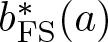 $b^*_{\mathrm{FS}}(a)$ so that
 $c_{a,b} \lt \Lambda_*$.
2.2. Existence of minimizers
Following the arguments in [Reference König20], we start by introducing some notations. Hereafter, in order to shorten formulas, for each  $u\in \mathcal{D}^{1,2}_{a}(\mathbb{R}^N)$, we denote
 \begin{equation}
\|u\|:
=\left(\int_{\mathbb{R}^N}|x|^{-2a}|\nabla u|^2 \mathrm{d}x\right)^{1/2},
\quad \|u\|_*: =\left(\int_{\mathbb{R}^N}|x|^{-qb}|u|^{q} \mathrm{d}x\right)^{1/2}.
\end{equation}
We denote the standard  $\|\cdot\|_*$-normalized Talenti type bubble by
 \begin{equation}
B(x)=\mathcal{B}\left(1+|x|^{(a_c-a)(q-2)}\right)
^{-\frac{2}{q-2}},
\end{equation}
with  $\mathcal{B} \gt 0$ chosen such that
 $\|B\|_*=1$. As usual,
 $B_\lambda(x):=\lambda^{a_c-a}B(\lambda x)$ for λ > 0. Notice that for all λ > 0,
 \begin{equation*}
\|B_\lambda\|_*=\|B\|_*=1,\quad \|B_\lambda\|^2=\mathcal{S}_{a,b},\quad -\mathrm{div}(|x|^{-2a}\nabla B_\lambda)=\mathcal{S}_{a,b}|x|^{-bq} B_\lambda^{q-1}.
\end{equation*}
We denote by
 \begin{equation*}
\mathcal{M}_{a,b}^1:=\{B_\lambda: \lambda \gt 0\}\subset \mathcal{M}_{a,b}
\end{equation*}
the submanifold of  $\mathcal{M}_{a,b}$ consisting of
 $\|\cdot\|_*$-normalized Talenti type bubbles.
It does not seem clear whether the functional  $\mathcal{E}$ defined as in (1.14) decreases or increases under rearrangement. The next lemma gives a convenient reformulation of the distant
 $\mathrm{dist}(u,\mathcal{M}_{a,b})$ in terms of a new optimization problem
 \begin{equation}
\mathrm{\mathbf{m}}(u):=\sup_{v\in \mathcal{M}_{a,b}^1}(u,|x|^{-qb}v^{q-1})^2.
\end{equation}
Here,
 \begin{equation*}
(u,|x|^{-qb}v^{q-1})
=\int_{\mathbb{R}^N}|x|^{-qb}v^{q-1}u\mathrm{d}x
\end{equation*}
denotes the pairing between  $L^q(\mathbb{R}^N;|x|^{-qb}\mathrm{d}x)$ and its dual. Hereafter, we will mostly work with this reformulation when proving our results below.
Lemma 2.1. For each  $u\in \mathcal{D}^{1,2}_{a}(\mathbb{R}^N)\setminus \mathcal{M}_{a,b}$, it holds that
 \begin{align}
\mathrm{dist}(u,\mathcal{M}_{a,b})^2
=\|u\|^2-\mathcal{S}_{a,b}\mathrm{\mathbf{m}}(u).
\end{align}
Moreover,  $\mathrm{dist}(u,\mathcal{M}_{a,b})$ can always be achieved. The function
 $(u,|x|^{-qb}v^{q-1})v$ optimizes
 $\mathrm{dist}(u,\mathcal{M}_{a,b})$ if and only if
 $v\in \mathcal{M}_{a,b}^1$ optimizes
 $\mathrm{\mathbf{m}}(u)$.
Proof. For any  $v\in \mathcal{M}_{a,b}^1$ and
 $c\in\mathbb{R}$, we have
 \begin{align*}
\|u-cv\|^2
& =
\|u\|^2-2c\mathcal{S}_{a,b}(u,|x|^{-qb}v^{q-1})
+c^2\mathcal{S}_{a,b}
\\
& = \|u\|^2-\mathcal{S}_{a,b}(u,|x|^{-qb}v^{q-1})^2
+\mathcal{S}_{a,b}\left(c-(u,|x|^{-qb}v^{q-1})\right)^2,
\end{align*}
thanks to  $-\mathrm{div}(|x|^{-2a}\nabla v)=\mathcal{S}_{a,b}|x|^{-bq} v^{q-1}$. Hence
 \begin{align*}
\mathrm{dist}(u,\mathcal{M}_{a,b})^2
= & \inf_{v\in \mathcal{M}_{a,b}^1}\inf_{c\in\mathbb{R}}
\|u-cv\|^2
=\|u\|^2-\mathcal{S}_{a,b}\sup_{v\in\mathcal{M}_{a,b}^1}
(u,|x|^{-qb}v^{q-1})^2,
\end{align*}
which proves (2.9). The relation between the optimizers of  $\mathrm{dist}(u,\mathcal{M}_{a,b})$ and
 $\mathrm{\mathbf{m}}(u)$ is now immediate from the fact that
 \begin{equation*}
\inf_{c\in\mathbb{R}}
\left(c-(u,|x|^{-qb}v^{q-1})\right)^2
\end{equation*}
is attained uniquely at  $c=(u,|x|^{-qb}v^{q-1})$.
By this relation between optimizers, it only remains to prove that  $\mathrm{\mathbf{m}}(u)$ can always be achieved. Let us first consider the case
 $\mathrm{\mathbf{m}}(u) \gt 0$. Let
 $\{B_{\lambda_n}\}$ be a minimizing sequence for
 $\mathrm{\mathbf{m}}(u)$. This sequence converges to some
 $B_{\lambda_0}$, which plainly is a minimizer, unless
 $\lambda_n\to 0$ or
 $\lambda_n\to \infty$ as
 $n\to \infty$. As in the proof of [Reference Wei and Wu25, Proposition 4.1], in these two cases, it is not difficult to verify that
 $(u,|x|^{-qb}B_{\lambda_n}^{q-1})=\mathcal{S}_{a,b}^{-1}\langle u, B_{\lambda_n}\rangle_{\mathcal{D}^{1,2}_a(\mathbb{R}^N)} \to 0$ as
 $n\to \infty$, which leads to a contradiction. While for the case
 $\mathrm{\mathbf{m}}(u)=0$, then we must have
 $(u,|x|^{-qb}v^{q-1})=0$ for all
 $v\in\mathcal{M}_{a,b}^1$, thus
 $\mathrm{\mathbf{m}}(u)$ can be achieved by any
 $v\in\mathcal{M}_{a,b}^1$. The proof is completed.
As a consequence of (2.2), together with some further analysis, we are going to show that there is a minimizer of the best stability constant  $c_{a,b}$. Let
 $\{u_n\}\subset \mathcal{D}^{1,2}_{a}(\mathbb{R}^N)
\setminus \mathcal{M}_{a,b}$ be a
 $\|\cdot\|_*$-normalized minimizing sequence for
 $c_{a,b}$ satisfying
 \begin{align}
\mathcal{E}(u_n)=c_{a,b}+o_n(1),\quad \|u_n\|_*=1.
\end{align}
Here  $o_n(1)$ denotes that
 $o_n(1)\to 0$ as
 $n\to \infty$. Then
 \begin{align*}
\|u_n\|^2=(c_{a,b}+o_n(1))
\mathrm{dist}(u_n,\mathcal{M}_{a,b})^2
+\mathcal{S}_{a,b}
\leq (c_{a,b}+o_n(1))\|u_n\|^2
+\mathcal{S}_{a,b},
\end{align*}
and (2.2) indicates  $c_{a,b} \lt 2-2^{\frac{2}{q}} \lt 1$ due to q > 2, thus
 $\{u_n\}$ is bounded in
 $\mathcal{D}^{1,2}_{a}(\mathbb{R}^N)$. By a theorem of Lions [Reference Lions21] (see also [Reference Catrina and Wang7, Lemma 4.1]), up to scalings, we may assume that
 $u_n\rightharpoonup u_0$ weakly in
 $\mathcal{D}^{1,2}_{a}(\mathbb{R}^N)$. Letting
 $v_n:=u_n-u_0$, we can thus rewrite
 \begin{equation}u_n = v_n + u_0\;\text{for some}\;u_0\in\mathcal D_a^{1,2}(\mathbb{R}^N),\quad v_n \rightharpoonup 0 \;\text{weakly in}\;\mathcal D_a^{1,2}(\mathbb{R}^N).\end{equation}
We first check that if the convergence is strong, then a minimizer of  $c_{a,b}$ must exist.
Proposition 2.2. Let  $\{u_n\}\subset\mathcal D_a^{1,2}(\mathbb{R}^N)\setminus{\mathcal M}_{a,b}$ satisfy (2.10) and (2.11) and suppose that
 $v_n\to 0$ strongly in
 $\mathcal{D}^{1,2}_{a}(\mathbb{R}^N)$. Then
 $\textstyle u_0\in\mathcal D_a^{1,2}(\mathbb{R}^N)\setminus{\mathcal M}_{a,b}$ is a minimizer of
 $c_{a,b}$.
Proof. If  $v_n\to 0$ strongly in
 $\mathcal{D}^{1,2}_{a}(\mathbb{R}^N)$, that is,
 $u_n\to u_0$ strongly in
 $\mathcal{D}^{1,2}_{a}(\mathbb{R}^N)$, then it is clear that
 $\|u_n\|^2\to \|u_0\|^2$. By CKN inequality (1.6), it also holds that
 $\|u_n\|^2_*\to \|u_0\|^2_*$ due to
 $0\leq |\|u_n\|_*-\|u_0\|_*|\leq \|u_n-u_0\|_*\to 0$. Note that by Hölder’s inequality, we have
 \begin{align*}
& \sup_{\lambda \gt 0}\left|(u_n,|x|^{-qb}B_\lambda^{q-1})^2-
(u_0,|x|^{-qb}B_\lambda^{q-1})^2\right|
\\
& = \sup_{\lambda \gt 0}
\left|\int_{\mathbb{R}^N}|x|^{-qb}B_\lambda^{q-1}(u_n+u_0)
\mathrm{d}x
\int_{\mathbb{R}^N}|x|^{-qb}B_\lambda^{q-1}(u_n-u_0)
\mathrm{d}x
\right|
\\
& \leq \|u_n+u_0\|_*\|u_n-u_0\|_*
\leq (1+\|u_0\|_*)\|u_n-u_0\|_*\to 0,
\end{align*}
and from the definition of  $\mathrm{\mathbf{m}}$ as in (2.8),
 \begin{align*}
& \mathrm{\mathbf{m}}(u_n)
\leq \mathrm{\mathbf{m}}(u_0)
+\sup_{\lambda \gt 0}\left[(u_n,|x|^{-qb}B_\lambda^{q-1})^2-
(u_0,|x|^{-qb}B_\lambda^{q-1})^2\right],\\
& \mathrm{\mathbf{m}}(u_0)
\leq \mathrm{\mathbf{m}}(u_n)
+\sup_{\lambda \gt 0}\left[(u_0,|x|^{-qb}B_\lambda^{q-1})^2-
(u_n,|x|^{-qb}B_\lambda^{q-1})^2\right],
\end{align*}
due to  $\sup P\leq \sup Q+\sup(P-Q)$, then we can deduce that
 $\mathrm{\mathbf{m}}(u_n)
\to \mathrm{\mathbf{m}}(u_0)$. Thus from lemma 2.1, we also have
 $\mathrm{dist}(u_n,\mathcal{M}_{a,b})^2\to \mathrm{dist}(u_0,\mathcal{M}_{a,b})^2$. Therefore,
 $\mathcal{E}(u_n)\to \mathcal{E}(u_0)$, and u 0 is a minimizer provided
 $u_0\notin \mathcal{M}_{a,b}$, i.e.,
 $\mathrm{dist}(u_0,\mathcal{M}_{a,b})\neq 0$.
But for sequence  $\{u_n\}$ such that
 $\mathrm{dist}(u_n,\mathcal{M}_{a,b})\to 0$ satisfying
 $\|u_n\|\geq \mathcal{S}_{a,b}^{1/2}\|u_n\|_*=\mathcal{S}_{a,b}^{1/2}$, it is known from (1.19) that
 $\liminf\limits_{n\to\infty}\mathcal{E}(u_n)\geq \Lambda_*$, which leads to a contradiction with
 $c_{a,b} \lt \Lambda_*$. Hence the minimizing sequence
 $\{u_n\}$ cannot satisfy
 $\mathrm{dist}(u_n,\mathcal{M}_{a,b})\to 0$. As explained above, the proof is now completed.
Therefore, proposition 2.2 indicates that the proof of theorem 1.1 now consists in showing that  $v_n\to 0$ strongly in
 $\mathcal{D}^{1,2}_{a}(\mathbb{R}^N)$ must, in fact, be the case.
To do so, let us investigate how the components of  $\mathcal{E}(u_n)$ behave under the decomposition (2.11). It is standard to check that the weak convergence implies
 \begin{align}
\|u_n\|^2=\|u_0\|^2+\|v_n\|^2+o_n(1),
\end{align}
and the Brézis–Lieb lemma [Reference Brézis and Lieb3] indicates
 \begin{align}
1=\|u_n\|^q_*=\|u_0\|^q_*+\|v_n\|^q_*+o_n(1).
\end{align}
The following lemma gives the important information on how the distance  $\mathrm{dist}(u_n,\mathcal{M}_{a,b})^2$ decomposes. Recall that by definition
 $\mathrm{\mathbf{m}}(u):=\sup_{v\in \mathcal{M}_{a,b}^1}(u,|x|^{-qb}v^{q-1})^2$.
Lemma 2.3. Let  $\{u_n\}\subset \mathcal{D}^{1,2}_{a}(\mathbb{R}^N)
\setminus \mathcal{M}_{a,b}$ satisfy (2.10) and (2.11), then it holds that
 \begin{align}
\mathrm{\mathbf{m}}(u_n)=\max\{\mathrm{\mathbf{m}}(u_0),
\mathrm{\mathbf{m}}(v_n)\}+o_n(1).
\end{align}
In particular,
 \begin{align}
\mathrm{dist}(u_n,\mathcal{M}_{a,b})^2
=\|u_0\|^2+\|v_n\|^2
-\mathcal{S}_{a,b}\max\{\mathrm{\mathbf{m}}(u_0),
\mathrm{\mathbf{m}}(v_n)\}+o_n(1).
\end{align}
Proof. We follow the arguments in [Reference König20]. By lemma 2.1,  $\mathrm{\mathbf{m}}(u_n)$ has an optimizer
 $B_{\lambda_n}\in \mathcal{M}_{a,b}^1$. We consider two different cases.
Suppose first that λn is bounded away from zero and infinity. Then up to a subsequence  $\lambda_n \to \lambda_0$ for some
 $\lambda_0\in (0,\infty)$, and consequently
 $B_{\lambda_n}\to B_{\lambda_0}$ strongly in
 $L^q(\mathbb{R}^N;|x|^{-qb}\mathrm{d}x)$. But this implies
 $(v_n,|x|^{-qb}B_{\lambda_n}^{q-1})\to 0$ by weak convergence
 $v_n\rightharpoonup 0$. Thus
 \begin{align}
\mathrm{\mathbf{m}}(u_n)
& = \left((u_0,|x|^{-qb}B_{\lambda_n}^{q-1})
+(v_n,|x|^{-qb}B_{\lambda_n}^{q-1})\right)^2
=(u_0,|x|^{-qb}B_{\lambda_n}^{q-1})^2
+o_n(1) \nonumber
\\
& \leq \mathrm{\mathbf{m}}(u_0)+o_n(1).
\end{align}
In the remaining, second case, we have  $\lambda_n\to 0$ or
 $\lambda_n\to \infty$ along a subsequence. As in the proof of [Reference Wei and Wu25, Proposition 4.1], this can be easily checked to yield
 \begin{equation*}
(u_0,|x|^{-qb}B_{\lambda_n}^{q-1})
=\mathcal{S}_{a,b}^{-1}\langle u_0,B_{\lambda_n}\rangle_{\mathcal{D}^{1,2}_a(\mathbb{R}^N)}\to 0,
\end{equation*}
thus we get
 \begin{align}
\mathrm{\mathbf{m}}(u_n)
= (v_n,|x|^{-qb}B_{\lambda_n}^{q-1})^2
+o_n(1)
\leq \mathrm{\mathbf{m}}(v_n)+o_n(1).
\end{align}
Combining (2.16) and (2.17), we obtain
 \begin{align}
\mathrm{\mathbf{m}}(u_n)
\leq \max\{\mathrm{\mathbf{m}}(u_0),\mathrm{\mathbf{m}}(v_n)\}
+o_n(1),
\end{align}
at least along some subsequence. But our argument shows that from any subsequence we can extract another subsequence such that the inequality (2.18) holds. Thus, (2.18) must in fact hold for the entire sequence  $\{u_n\}$.
In order to establish (2.14), we will now prove the converse inequality by a similar argument. If  $\mathrm{\mathbf{m}}(u_0)=0$, then it is trivial that
 $\mathrm{\mathbf{m}}(u_n)
\geq \mathrm{\mathbf{m}}(u_0)+o_n(1)$. The other case is
 $\mathrm{\mathbf{m}}(u_0) \gt 0$, thus from lemma 2.1, we let
 $B_{\lambda_{u_0}}$ be an optimizer for
 $\mathrm{\mathbf{m}}(u_0)$, then
 $(v_n,|x|^{-qb}B_{\lambda_{u_0}}^{q-1})\to 0$ by weak convergence
 $v_n\rightharpoonup 0$, and thus
 \begin{align}
\mathrm{\mathbf{m}}(u_n)
\geq (u_n,|x|^{-qb}B_{\lambda_{u_0}}^{q-1})^2
= (u_0,|x|^{-qb}B_{\lambda_{u_0}}^{q-1})^2
+o_n(1)
= \mathrm{\mathbf{m}}(u_0)+o_n(1).
\end{align}
If  $\mathrm{\mathbf{m}}(v_n)\to 0$ along some subsequence, then
 $\mathrm{\mathbf{m}}(u_n)
\geq \mathrm{\mathbf{m}}(v_n)+o_n(1)$. The other case is
 $\mathrm{\mathbf{m}}(v_n) \gt 0$ as n sufficiently large, then let
 $B_{\lambda_{v_n}}$ be an optimizer for
 $\mathrm{\mathbf{m}}(v_n)$. Suppose first that
 $\lambda_{v_n} \to 0$ or
 $\lambda_{v_n}\to \infty$ along a subsequence. Then, as above
 $(u_0,|x|^{-qb}B_{\lambda_{v_n}}^{q-1})\to 0$, thus we obtain in that case
 \begin{align}
\mathrm{\mathbf{m}}(u_n)
\geq (u_n,|x|^{-qb}B_{\lambda_{v_n}}^{q-1})^2
= (v_n,|x|^{-qb}B_{\lambda_{v_n}}^{q-1})^2
+o_n(1)
= \mathrm{\mathbf{m}}(v_n)+o_n(1).
\end{align}
If, on the other hand,  $\{\lambda_{v_n}\}$ is bounded away from zero and infinity, then up to a subsequence
 $\lambda_{v_n}\to \lambda_{v_0}$ for some
 $\lambda_{v_0}\in (0,\infty)$. But then
 $\mathrm{\mathbf{m}}(v_n)= (v_n,|x|^{-qb}B_{\lambda_{v_n}}^{q-1})^2 \to 0$ by weak convergence
 $v_n\rightharpoonup 0$, and so (2.20) holds trivially.
By the same remark as in the first part of the proof, (2.20) holds in fact along the whole sequence  $\{u_n\}$. Now, combining (2.19) with (2.20) and (2.18), the inequality (2.14) follows.
Finally, (2.15) is immediate from lemma 2.1 together with (2.12) and (2.14).
The next lemma serves as an important preparation for our main argument. Contrary to (2.12), (2.13), and (2.14), here the minimizing property of  $\{u_n\}$ comes into play.
Lemma 2.4. Let  $\{u_n\}\subset \mathcal{D}^{1,2}_{a}(\mathbb{R}^N)
\setminus \mathcal{M}_{a,b}$ satisfy (2.10) and (2.11). If there is a constant
 $c_0 \gt 0$ such that
 $\|v_n\|\geq c_0$ when
 $n$ is sufficiently large, then
 $\lim_{n\to \infty}\mathrm{\mathbf{m}}(v_n)=
\mathrm{\mathbf{m}}(u_0)$.
Proof. Assume firstly that, up to extracting a subsequence, still labelled by  $\{v_n\}$,
 \begin{align}
\lim_{n\to \infty}\mathrm{\mathbf{m}}(v_n) \gt \mathrm{\mathbf{m}}(u_0).
\end{align}
Note that (2.21) implies
 \begin{equation*}
0 \lt \lim\limits_{n\to \infty}\mathrm{\mathbf{m}}(v_n)
\leq \lim\limits_{n\to \infty}\|v_n\|^2_*,
\end{equation*}
then combining with (2.13) we deduce that  $\{\|v_n\|_*\}$ is bounded away from zero and infinity for n sufficiently large. Multiplying by a constant, we may equivalently consider
 \begin{equation*}
\tilde{u}_n=\frac{v_n}{\|v_n\|_*}+\frac{u_0}{\|v_n\|_*}
=: \tilde{v}_n+ \tilde{u}_{0n}, \quad\mbox{with}\ \|\tilde{v}_n\|_*=1.
\end{equation*}
Then by (2.12), (2.13), and lemma 2.1, we have
 \begin{align*}
\mathcal{E}(\tilde{u}_n)
& =
\frac{\|\tilde{u}_n\|^2-\mathcal{S}_{a,b}\|\tilde{u}_n\|^2_*}
{\mathrm{dist}(\tilde{u}_n,\mathcal{M}_{a,b})^2}\\
& = \frac{\|\tilde{v}_n\|^2-\mathcal{S}_{a,b}+\|\tilde{u}_{0n}\|^2
-\mathcal{S}_{a,b}\left[
\left(1+\|\tilde{u}_{0n}\|^q_*\right)^{\frac{2}{q}}-1\right]}
{\|\tilde{v}_n\|^2
+\|\tilde{u}_{0n}\|^2
-\mathcal{S}_{a,b}\mathrm{\mathbf{m}}(\tilde{u}_{n})}
+o_n(1)
\\
& = \frac{\|\tilde{v}_n\|^2-\mathcal{S}_{a,b}+\|\tilde{u}_{0n}\|^2
-\mathcal{S}_{a,b}\left[
\left(1+\|\tilde{u}_{0n}\|^q_*\right)^{\frac{2}{q}}-1\right]}
{\|\tilde{v}_n\|^2
-\mathcal{S}_{a,b}\mathrm{\mathbf{m}}(\tilde{v}_{n})
+\|\tilde{u}_{0n}\|^2}
+o_n(1),
\end{align*}
thanks to the assumption (2.21) and lemma 2.3 imply  $\mathrm{\mathbf{m}}(\tilde{u}_{n})
=\mathrm{\mathbf{m}}(\tilde{v}_{n})+o_n(1)$. Our goal is now to estimate the quotient using [Reference König20, Lemma 2.4].
Suppose for the moment that  $\tilde{v}_{n}\notin \mathcal{M}_{a,b}$ for n sufficiently large. Set
 \begin{align*}
\bar{A}& := \lim_{n\to \infty}\|\tilde{v}_n\|^2-\mathcal{S}_{a,b},\quad \bar{B}:=\lim_{n\to \infty}\left[\|\tilde{v}_n\|^2- \mathcal{S}_{a,b}\mathrm{\mathbf{m}}(\tilde{v}_{n})\right],
\\
\bar{C}& := \lim_{n\to \infty}
\left\{\|\tilde{u}_{0n}\|^2
-\mathcal{S}_{a,b}\left[
\left(1+\|\tilde{u}_{0n}\|^q_*\right)^{\frac{2}{q}}-1\right]
\right\},\quad
\bar{D}:=\lim_{n\to \infty}\|\tilde{u}_{0n}\|^2.
\end{align*}
Notice that  $\bar{A}, \bar{B}, \bar{C}, \bar{D} \gt 0$, since we have assumed that
 $\tilde{v}_{n}\notin \mathcal{M}_{a,b}$ for n sufficiently large and
 $\|\tilde{u}_{0n}\|$ is bounded away from zero. Since
 \begin{equation*}
c_{a,b}=\lim_{n\to \infty}\mathcal{E}(u_n)=\lim_{n\to \infty}\mathcal{E}(\tilde{u}_n)=\frac{\bar{A}+\bar{C}}{\bar{B}+\bar{D}}
\end{equation*}
and
 \begin{equation*}
\frac{\bar{A}}{\bar{B}}=\lim\limits_{n\to \infty}\mathcal{E}(\tilde{v}_n)=\lim\limits_{n\to \infty}\mathcal{E}(v_n)\geq c_{a,b},
\end{equation*}
we must have  $\bar{C}/\bar{D}\leq c_{a,b}$, then
 $\bar{A}/\bar{B}\geq \bar{C}/\bar{D}$. Now, if
 $\mathrm{\mathbf{m}}(u_0) \gt 0$ we let Fn be the scalar multiple of
 $\tilde{u}_{0n}$ such that
 $\mathrm{\mathbf{m}}(F_{n})
=\mathrm{\mathbf{m}}(\tilde{v}_{n})$, that is,
 $F_n=c_n\tilde{u}_{0n}$ where
 $c_n^2=\mathrm{\mathbf{m}}(\tilde{v}_{n})/
\mathrm{\mathbf{m}}(\tilde{u}_{0n})
=\mathrm{\mathbf{m}}(v_{n})/ \mathrm{\mathbf{m}}(u_0)$, while if
 $\mathrm{\mathbf{m}}(u_0)=0$ we let
 $F_n=c\tilde{u}_{0n}$ for any c > 1. Then, as a consequence of (2.21), we have
 \begin{equation*}
\lim\limits_{n\to \infty}\|F_n\|_* \gt \lim\limits_{n\to \infty}\|\tilde{u}_{0n}\|_*.
\end{equation*}
By [Reference König20, Lemma 2.3], which states that
 \begin{align}
\mbox{the function}\ \eta\mapsto \frac{(1+\eta^q)^{\frac{2}{q}}-1}{\eta^2}\ \mbox{is strictly increasing in}\ \eta\in(0,\infty),
\end{align}
so that
 \begin{align*}
\frac{\bar{C}}{\bar{D}}
= 1-\lim_{n\to \infty}\frac{\mathcal{S}_{a,b}\left[
\left(1+\|\tilde{u}_{0n}\|^q_*\right)^{\frac{2}{q}}-1\right]
}{S_{[\tilde{u}_{0n}]}\|\tilde{u}_{0n}\|^2_*} \gt 1-\lim_{n\to \infty}\frac{\mathcal{S}_{a,b}\left[
\left(1+\|F_n\|^q_*\right)^{\frac{2}{q}}-1\right]
}{S_{[\tilde{u}_{0n}]}\|F_n\|^2_*}
=:\frac{\bar{E}}{\bar{F}},
\end{align*}
where  $S_{[\tilde{u}_{0n}]}
=\|\tilde{u}_{0n}\|^2/\|\tilde{u}_{0n}\|^2_*$, and
 \begin{align*}
\bar{E}=\lim\limits_{n\to \infty}\left\{S_{[\tilde{u}_{0n}]}\|F_n\|^2_*-\mathcal{S}_{a,b}\left[
\left(1+\|F_n\|^q_*\right)^{\frac{2}{q}}-1\right]\right\},
\quad
\bar{F}=\lim\limits_{n\to \infty}S_{[\tilde{u}_{0n}]}\|F_n\|^2_*.
\end{align*}
By lemma 2.3, it is not difficult to verify that  $\mathrm{\mathbf{m}}(F_n+\tilde{v}_n)
=\mathrm{\mathbf{m}}(\tilde{v}_n)+o_n(1)$, thus we have
 \begin{align*}
\lim\limits_{n\to \infty}\mathcal{E}(F_n+\tilde{v}_n)
=\frac{\bar{A}+\bar{E}}{\bar{B}+\bar{F}}.
\end{align*}
Note that  $\bar{D}\leq \bar{F}$, then since
 $\bar{A}/\bar{B}\geq \bar{C}/\bar{D} \gt \bar{E}/\bar{F}$, from [Reference König20, Lemma 2.4] we obtain
 \begin{align*}
c_{a,b}
=\lim\limits_{n\to \infty}\mathcal{E}(u_n)
=\lim\limits_{n\to \infty}\mathcal{E}(\tilde{u}_n)
=\frac{\bar{A}+\bar{C}}{\bar{B}+\bar{D}} \gt \frac{\bar{A}+\bar{E}}{\bar{B}+\bar{F}}
=\lim\limits_{n\to \infty}\mathcal{E}(F_n+\tilde{v}_n).
\end{align*}
But this contradicts the definition of  $c_{a,b}$. Hence (2.21) is impossible.
If, on the other hand,  $\tilde{v}_{n}\in \mathcal{M}_{a,b}$ along some subsequence, then
 $\bar{A}=\bar{B}=0$ in the above and we directly conclude a contradiction in the same way from
 $\bar{C}/\bar{D} \gt \bar{E}/\bar{F}$.
The remaining case to treat is that where, up to a subsequence,
 \begin{align*}
\mathrm{\mathbf{m}}(u_0) \gt \lim_{n\to \infty}\mathrm{\mathbf{m}}(v_n).
\end{align*}
But here one arrives at a contradiction in a similar fashion, with the roles of u 0 and vn reversed and considering
 \begin{equation*}
\hat{u}_n=\frac{v_n}{\|u_0\|_*}+\frac{u_0}{\|u_0\|_*}
=: \hat{v}_n+ \hat{u}_{0}, \quad\mbox{with}\ \|\hat{u}_{0}\|_*=1.
\end{equation*}
The fact that  $\hat{D}:=\lim\limits_{n\to \infty}\|\hat{v}_{n}\|^2=\lim\limits_{n\to \infty}\|v_{n}\|^2/\|u_0\|_*^2 \gt 0$ is guaranteed here by assumption. The rest of the proof is identical to the above.
We are now ready to prove the existence of minimizers of  $c_{a,b}$.
Proof of theorem 1.1
Let  $\{u_n\}\in \mathcal{D}^{1,2}_{a}(\mathbb{R}^N)
\setminus \mathcal{M}_{a,b}$ satisfy (2.10) and (2.11). Suppose for contradiction that
 $v_n=u_n-u_0$ does not converge strongly to zero in
 $\mathcal{D}^{1,2}_{a}(\mathbb{R}^N)$. Then, after passing to a subsequence, still labelled by
 $\{v_n\}$, then we have
 $\|v_n\|\geq c_0$ for some
 $c_0 \gt 0$. Thus, lemma 2.4 indicates
 \begin{align}
\mathrm{\mathbf{m}}(u_0)=
\mathrm{\mathbf{m}}(v_n)+o_n(1).
\end{align}
Suppose first that  $\|v_n\|_*\leq \|u_0\|_*+o_n(1)$. As in the proof of lemma 2.4, let us consider
 \begin{equation*}
\hat{u}_n=\frac{v_n}{\|u_0\|_*}+\frac{u_0}{\|u_0\|_*}
=: \hat{v}_n+ \hat{u}_0, \quad\mbox{with}\ \|\hat{u}_0\|_*=1.
\end{equation*}
Thanks to (2.23) and lemma 2.3, we can write
 \begin{align*}
\mathrm{dist}(\hat{u}_n,\mathcal{M}_{a,b})^2
=\|\hat{u}_0\|^2
-\mathcal{S}_{a,b}\mathrm{\mathbf{m}}(\hat{u}_0)
+\|\hat{v}_n\|^2+o_n(1).
\end{align*}
Together (2.12) with (2.13) and lemma 2.1, we deduce that
 \begin{align*}
c_{a,b}+o_n(1)
= \frac{\|\hat{u}_0\|^2-\mathcal{S}_{a,b}+\|\hat{v}_{n}\|^2
-\mathcal{S}_{a,b}\left[
\left(1+\|\hat{v}_{n}\|^q_*\right)^{\frac{2}{q}}-1\right]}
{\|\hat{u}_0\|^2
-\mathcal{S}_{a,b}\mathrm{\mathbf{m}}(\hat{u}_0)
+\|\hat{v}_{n}\|^2}.
\end{align*}
Similar to the proof of lemma 2.4, by the definition of  $c_{a,b}$ that
 \begin{align*}
c_{a,b}\leq \mathcal{E}(\hat{u}_0)
= \frac{\|\hat{u}_0\|^2-\mathcal{S}_{a,b}}
{\|\hat{u}_0\|^2
-\mathcal{S}_{a,b}\mathrm{\mathbf{m}}(\hat{u}_0)},\quad \mbox{if}\ \hat{u}_0\not\in \mathcal{M}_{a,b},
\end{align*}
and
 \begin{align*}
c_{a,b}+o_n(1)
= \frac{\|\hat{v}_{n}\|^2
-\mathcal{S}_{a,b}\left[
\left(1+\|\hat{v}_{n}\|^q_*\right)^{\frac{2}{q}}-1\right]}
{\|\hat{v}_{n}\|^2},\quad \mbox{if}\ \hat{u}_0\in \mathcal{M}_{a,b}.
\end{align*}
Anyway,
 \begin{align*}
c_{a,b}+o_n(1)
\geq \frac{\|\hat{v}_{n}\|^2
-\mathcal{S}_{a,b}\left[
\left(1+\|\hat{v}_{n}\|^q_*\right)^{\frac{2}{q}}-1\right]}
{\|\hat{v}_{n}\|^2}
=1-\frac{\mathcal{S}_{a,b}\left[
\left(1+\|\hat{v}_n\|^q_*\right)^{\frac{2}{q}}-1\right]
}{S_{[\hat{v}_{n}]}\|\hat{v}_n\|^2_*},
\end{align*}
thanks to (2.23) implies that  $\{\|\hat{v}_n\|_*\}$ is bounded away from zero for n sufficiently large, where
 $S_{[\hat{v}_{n}]}
=\|\hat{v}_{n}\|^2/\|\hat{v}_{n}\|^2_*$. Note that the assumption
 $\|v_n\|_*\leq \|u_0\|_*+o_n(1)$ implies
 $\|\hat{v}_n\|_*\leq 1+o_n(1)$, then from (2.22) we must have
 \begin{align*}
c_{a,b}
\geq 1-\frac{\mathcal{S}_{a,b}\left(
2^{\frac{2}{q}}-1\right)
}{S_{[\hat{v}_{n}]}}+o_n(1).
\end{align*}
Since we know by (2.2) that  $c_{a,b} \lt 2-2^{\frac{2}{q}}$ with strict inequality, then we find, for n sufficiently large, that
 \begin{align}
1-\frac{\mathcal{S}_{a,b}\left(
2^{\frac{2}{q}}-1\right)
}{S_{[\hat{v}_{n}]}} \lt 2-2^{\frac{2}{q}},
\end{align}
which is equivalent to  $S_{[\hat{v}_{n}]} \lt \mathcal{S}_{a,b}$. But this contradicts the definition of
 $\mathcal{S}_{a,b}$.
If we assume instead the reverse inequality  $\|u_0\|_*\leq \|v_n\|_* +o_n(1)$, then we obtain a contradiction by writing
 \begin{align*}
\mathrm{dist}(u_n,\mathcal{M}_{a,b})^2
=\|u_0\|^2
+\|v_n\|^2
-\mathcal{S}_{a,b}\mathrm{\mathbf{m}}(v_n)
+o_n(1),
\end{align*}
thanks to (2.23) and lemma 2.3, and arguing in exactly the same way with the roles of u 0 and vn reversed.
Thus we have shown that vn must converge strongly to zero in  $\mathcal{D}^{1,2}_a(\mathbb{R}^N)$. By proposition 2.2, the proof of theorem 1.1 is now completed.
3. Upper bound of the CKN inequality
In this section, we are going to show the upper bound of the CKN inequality (1.6) in the all symmetry region (1.7).
Proof of theorem 1.2
From lemma 2.1, we know that for each  $u\in \mathcal{D}^{1,2}_{a}(\mathbb{R}^N)$,
 \begin{align}
\mathrm{dist}(u,\mathcal{M}_{a,b})^2
=\|u\|^2-\mathcal{S}_{a,b}\mathrm{\mathbf{m}}(u),
\end{align}
where  $\mathrm{\mathbf{m}}(u)=\sup_{v\in \mathcal{M}_{a,b}^1}
(\int_{\mathbb{R}^N}|x|^{-qb}v^{q-1}u\mathrm{d}x)^2$ and
 $\mathcal{M}_{a,b}^1=\{v\in \mathcal{M}_{a,b}: v \gt 0, \|v\|_*=1\}$. For each
 $v\in \mathcal{M}_{a,b}^1$, by Hölder’s inequality, we have
 \begin{align}
\left(\int_{\mathbb{R}^N}|x|^{-qb}v^{q-1}u\mathrm{d}x\right)^2
\leq \left(\int_{\mathbb{R}^N}|x|^{-qb}v^{q}\mathrm{d}x
\right)^{\frac{2(q-1)}{q}}
\left(\int_{\mathbb{R}^N}|x|^{-qb}|u|^q\mathrm{d}x
\right)^{\frac{2}{q}}
= \|u\|_*^2,
\end{align}
thus  $\mathrm{\mathbf{m}}(u)\leq \|u\|_*^2$ which implies that, there exists a constant
 $0 \lt \overline{c}\leq 1$ so that
 \begin{align}
\overline{c}\mathrm{dist}(u,\mathcal{M}_{a,b})^2
&\geq \int_{\mathbb{R}^N}|x|^{-2a}|\nabla u|^2 \mathrm{d}x
-\mathcal{S}_{a,b}\left(\int_{\mathbb{R}^N}|x|^{-qb}|u|^q \mathrm{d}x\right)^{\frac{2}{q}}, \nonumber \\
&\qquad\mbox{for all}\ u\in \mathcal{D}^{1,2}_{a}(\mathbb{R}^N).
\end{align}
Next, we show the sharp constant  $\overline{c}=1$. Consider the following eigenvalue problem
 \begin{equation}
-\mathrm{div}(|x|^{-2a}\rho)=\mu|x|^{-qb} U^{q-2}\rho \quad \mbox{in}\ \mathbb{R}^N,\quad \rho\in \mathcal{D}^{1,2}_{a}(\mathbb{R}^N).
\end{equation}
It is not difficult to verify that the embedding  $\mathcal{D}^{1,2}_{a}(\mathbb{R}^N)\hookrightarrow L^2(\mathbb{R}^N;|x|^{-qb} U^{q-2}\mathrm{d}x)$ is compact, thus the spectrums of (3.4) are discrete and satisfy
 \begin{align*}
\mu_1=1 \lt \mu_2\leq \mu_3\leq \cdots\leq \mu_k\to +\infty,\quad \mbox{as}\ k\to \infty.
\end{align*}
We denote ρk as the corresponding eigenfunction of µk. For each integer  $k\geq 2$, let us consider the test function sequence
 \begin{equation*}
\left\{u_n:=U+\epsilon_n\frac{\rho_k}{\|\rho_k\|}\right\},
\end{equation*}
where ϵn satisfies  $\epsilon_n\to 0^+$ as
 $n\to \infty$. Note that ρk and U are orthogonal in
 $\mathcal{D}^{1,2}_{a}(\mathbb{R}^N)$, i.e.,
 \begin{align*}
\int_{\mathbb{R}^N}|x|^{-2a}\nabla U\cdot \nabla \rho_k \mathrm{d}x=0.
\end{align*}
By Taylor’s expansion,
 \begin{align*}
\left|U+\epsilon_n\frac{\rho_k}{\|\rho_k\|}\right|^q
& =U^q+\frac{\epsilon_n q}{\|\rho_k\|}U^{q-1}\rho_k
+\frac{\epsilon_n^2 q(q-1)}{2\|\rho_k\|^2} U^{q-2}\rho_k^2+o\left(\frac{\epsilon_n^2}{\|\rho_k\|^2} U^{q-2}\rho_k^2\right),
\end{align*}
thus
 \begin{align}
\|u_n\|_*^2 & = \left[\|U\|_*^q
+\frac{\epsilon_n q}{\|\rho_k\|}\int_{\mathbb{R}^N}|x|^{-qb}U^{q-1}\rho_k\mathrm{d}x
+ \frac{q(q-1)\epsilon_n^2 }{2\|\rho_k\|^2}\right.\\
&\qquad\left.\int_{\mathbb{R}^N}|x|^{-qb}U^{q-2}\rho_k^2\mathrm{d}x
+o(\epsilon_n^2)\right]^{\frac{2}{q}}
\nonumber\\
&= \|U\|_*^2+ \frac{(q-1)\epsilon_n^2\|U\|_*^{2-q}}{\|\rho_k\|^2}
\int_{\mathbb{R}^N}|x|^{-qb}U^{q-2}\rho_k^2\mathrm{d}x
+o(\epsilon_n^2),
\end{align}
thanks to
 \begin{align*}
\int_{\mathbb{R}^N}|x|^{-qb}U^{q-1}\rho_k\mathrm{d}x
=\int_{\mathbb{R}^N}|x|^{-2a}\nabla U\cdot \nabla \rho_k \mathrm{d}x=0.
\end{align*}
Therefore,
 \begin{align*}
&\frac{\int_{\mathbb{R}^N}|x|^{-2a}|\nabla u_n|^2 \mathrm{d}x
-\mathcal{S}_{a,b}\left(\int_{\mathbb{R}^N}|x|^{-qb}|u_n|^q \mathrm{d}x\right)^{\frac{2}{q}}}
{\mathrm{dist}(u_n,\mathcal{M}_{a,b})^2}
\\
& \geq \frac{\|U\|^2+\epsilon_n^2
-\mathcal{S}_{a,b}\left[\|U\|_*^2+ \frac{(q-1)\epsilon_n^2\|U\|_*^{2-q}}{\|\rho_k\|^2}
\int_{\mathbb{R}^N}|x|^{-qb}U^{q-2}\rho_k^2\mathrm{d}x
+o(\epsilon_n^2)\right]}{\epsilon_n^2}
\\
& = 1-\frac{q-1}{\mu_k}+\frac{o(\epsilon_n^2)}{\epsilon_n^2}
\rightarrow 1-\frac{q-1}{\mu_k},
\end{align*}
as  $n\to \infty$, thanks to
 $\mathrm{dist}(u_n,\mathcal{M}_{a,b})^2\leq \epsilon_n^2$,
 $\mathcal{S}_{a,b}\|U\|_*^2=\|U\|^2=\|U\|_*^q$ and
 \begin{align*}
\|\rho_k\|^2
=\mu_k\int_{\mathbb{R}^N}|x|^{-qb}U^{q-2}\rho_k^2\mathrm{d}x.
\end{align*}
Now we deduce that  $\overline{c}\geq 1-\frac{q-1}{\mu_k}$ for all
 $k\geq 2$. Since k is arbitrary, letting
 $k\to \infty$ then
 $\mu_k\to \infty$, we have
 $\overline{c}\geq 1$. Then combining with
 $0 \lt \overline{c}\leq 1$, we have
 $\overline{c}=1$.
Finally, let us to show the equality in (3.3) with  $\overline{c}=1$ cannot hold for any
 $u\in \mathcal{D}^{1,2}_a(\mathbb{R}^N)\setminus\mathcal{M}_{a,b}$. If not, there is
 $\overline{u}\in \mathcal{D}^{1,2}_a(\mathbb{R}^N)\setminus\mathcal{M}_{a,b}$ such that
 \begin{align*}
\mathrm{dist}(\overline{u},\mathcal{M}_{a,b})^2
=\int_{\mathbb{R}^N}|x|^{-2a}|\nabla \overline{u}|^2 \mathrm{d}x
-\mathcal{S}_{a,b}\left(\int_{\mathbb{R}^N}|x|^{-qb}|\overline{u}|^q \mathrm{d}x\right)^{\frac{2}{q}},
\end{align*}
which is equivalent to  $\mathrm{\mathbf{m}}(\overline{u})= \|\overline{u}\|_*^2$. While from (3.2) we know that,
 $\mathrm{\mathbf{m}}(\overline{u})=\|\overline{u}\|_*^2$ if and only if
 $\overline{u}\in \mathcal{M}_{a,b}$, which leads to a contradiction. The proof of theorem 1.2 is completed.
Acknowledgements
S. Deng is partially supported by the National Natural Science Foundation of China (Grant 12371121). J. Wei is partially supported by the Hong Kong General Research Fund ‘New frontiers in singular limits of nonlinear partial differential equations’.
Appendix A. The numerical analysis
At first, we prove that there exists a unique solution  $K^* \gt 2$ of (1.22), and we also give the explicit form of
 $K^*$ by using the numerical analysis.
Lemma A.1. There exists a unique solution  $K^* \gt 2$ of (1.22); furthermore, by using the numerical analysis, we have
 $K^*\approx 6.698818$.
Proof. Let
 \begin{align*}
f(t):=2-2^{\frac{t-2}{t}}-\frac{4}{t+4},\quad \mbox{for}\ t \gt 2.
\end{align*}
It is equivalent to prove that f(t) has a unique zero point. It is obvious that
 \begin{align}
f(2)=\frac{1}{3} \gt 0,\quad \lim_{t\to\infty}f(t)=0.
\end{align}
By direct calculations, we have
 \begin{align*}
f'(t)
=-2^{\frac{t-2}{t}}\cdot\ln 2\cdot \frac{2}{t^2}+\frac{4}{(t+4)^2}
=\frac{2^{2-\frac{2}{t}}}{(t+4)^2}
\left[2^{\frac{2}{t}}
-\ln 2\cdot \left(\frac{t+4}{t}\right)^2\right].
\end{align*}
Let
 \begin{align*}
g(t):=2^{\frac{2}{t}}-\ln 2\cdot \left(\frac{t+4}{t}\right)^2,\quad \mbox{for}\ t \gt 2.
\end{align*}
It is obvious that
 \begin{align}
g(2)=2-9\ln 2
=2\left(1-\ln 2^{\frac{9}{2}}\right) \lt 0,\quad \lim_{t\to\infty}g(t)=1-\ln 2 \gt 0.
\end{align}
By direct calculations, we have
 \begin{align*}
g'(t)
=2^{\frac{2}{t}}\cdot\ln 2\cdot \left(-\frac{2}{t^2}\right)
-\ln 2\cdot 2\left(\frac{t+4}{t}\right)\left(-\frac{4}{t^2}\right)
=\frac{2\ln 2}{t^2}\left[4\left(\frac{t+4}{t}\right)-2^{\frac{2}{t}}\right].
\end{align*}
Since for all t > 2,
 \begin{align*}
4\left(\frac{t+4}{t}\right) \gt 4 \gt 2^{\frac{2}{t}},
\end{align*}
then we have  $g'(t) \gt 0$. Combining with (A.2) we deduce that, there is a unique
 $t^* \gt 2$ such that
 $g(t^*)=0$,
 $g(t) \lt 0$ for
 $t \lt t^*$, and
 $g(t) \gt 0$ for
 $t \gt t^*$. Therefore, f(t) is decreasing for
 $t \lt t^*$, and f(t) is increasing for
 $t \gt t^*$. Now, combining with (A.1) we deduce that, there is a unique
 $K^*\in (2,t^*)$ such that
 $f(K^*)=0$. By using the numerical analysis, we have
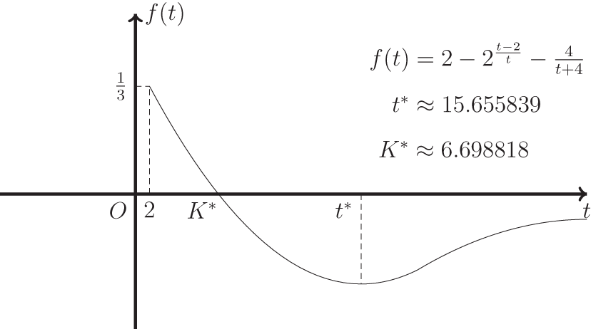
 $t^*\approx 15.655839$ and
 $K^*\approx 6.698818$. See Figure A.1 for the behaviour of the curve f(t).
The curve f(t) for t > 2.

Next, we give the numerical analysis about  $\epsilon_{N,a}$ obtained in §2.1. Let us consider the case N = 2, then
 $a_c=a_c^*=0$,
 $b_{\mathrm{FS}}(a)=\frac{-a}{\sqrt{a^2+1}}
+a$ and
 $b^*_{\mathrm{FS}}(a)=\frac{-2a}{-a+\sqrt{a^2+1}}+a$, furthermore,
 $a^*\approx-0.641866$.
Lemma A.2. Let  $N=2$. For each
 $a \lt a^*\approx-0.641866$, there exists a small
 $\epsilon_{a} \gt 0$ depending on a such that,
 $c_{a,b} \lt \Lambda_*$ for all
 $b\in [b^*_{\mathrm{FS}}(a)-\epsilon_a,b^*_{\mathrm{FS}}(a))$.
Proof. For each  $a \lt a^*$, let
 $b^*(a)$ be the solution of
 $\Lambda_*=2-2^{\frac{2}{q}}$ in
 $(b_{\mathrm{FS}}(a),b^*_{\mathrm{FS}}(a))$, i.e.,
 \begin{align}
\frac{\sqrt{a^2+1}\left(\sqrt{a^2+1}-\frac{a(1+a-b)}{b-a}\right)
-\frac{a^2(2+a-b)}{(b-a)^2}}
{\sqrt{a^2+1}\left(\sqrt{a^2+1}-\frac{a(1+a-b)}{b-a}\right)}
=2-2^{b-a},\quad b_{\mathrm{FS}}(a) \lt b \lt b^*_{\mathrm{FS}}(a).
\end{align}
Define
 \begin{align*}
f_a(b)
&:=\frac{\sqrt{a^2+1}\left(\sqrt{a^2+1}-\frac{a(1+a-b)}{b-a}\right)
-\frac{a^2(2+a-b)}{(b-a)^2}}
{\sqrt{a^2+1}\left(\sqrt{a^2+1}-\frac{a(1+a-b)}{b-a}\right)}\\
&=1+\frac{a^2}{\sqrt{a^2+1}}\cdot
\frac{b-a-2}{(\sqrt{a^2+1}+a)(b-a)^2-a(b-a)},
\end{align*}
and also
 \begin{align*}
g_a(t)
& :=\frac{t-2}{(\sqrt{a^2+1}+a)t^2-at},\quad t=b-a\in (b_{\mathrm{FS}}(a)-a,b^*_{\mathrm{FS}}(a)-a)\subset (0,1),
\end{align*}
then
 \begin{align*}
g_a'(t)
&=\left[(\sqrt{a^2+1}+a)t^2-at\right]^{-2}\\
&\qquad\left[-(\sqrt{a^2+1}+a)(t-2)^2+4(\sqrt{a^2+1}+a)t-2a\right] \gt 0,
\end{align*}
thanks to  $0 \lt t \lt 1$ and a < 0. Thus,
 $f_a(b)$ is strictly increasing for
 $b\in (a,a+1)$. It is obvious that the function
 $h_a(b):=2-2^{b-a}$ is strictly decreasing for
 $b\in (a,a+1)$. Note that at
 $b=b_{\mathrm{FS}}(a)$,
 \begin{align*}
f_a(b_{\mathrm{FS}}(a))=0,\quad h_a(b_{\mathrm{FS}}(a)) \gt h_a(a+1)=0.
\end{align*}
From (2.4) to (2.5) we know that  $a \lt a^*$ implies
 $b^*_{\mathrm{FS}}(a)-a \gt 1-\frac{2}{K^*}$, then at
 $b=b^*_{\mathrm{FS}}(a)$ we have
 $K\geq K^*$ where
 $K=\frac{2}{1+a-b}$, thus
 \begin{align*}
h_a(b^*_{\mathrm{FS}}(a))=2-2^{b^*_{\mathrm{FS}}(a)-a}
=2-2^{\frac{K-2}{K}}\leq \frac{4}{K+4}=f_a(b^*_{\mathrm{FS}}(a)).
\end{align*}
Therefore, there is a unique solution  $b^*(a)$ of
 $f_a(b)=h_a(b)$ for
 $b\in(b_{\mathrm{FS}}(a),b^*_{\mathrm{FS}}(a))$.
To sum up, for each  $a \lt a^*$, we choose
 $\epsilon_a=b^*_{\mathrm{FS}}(a)-b^*(a) \gt 0$ so that our lemma holds.
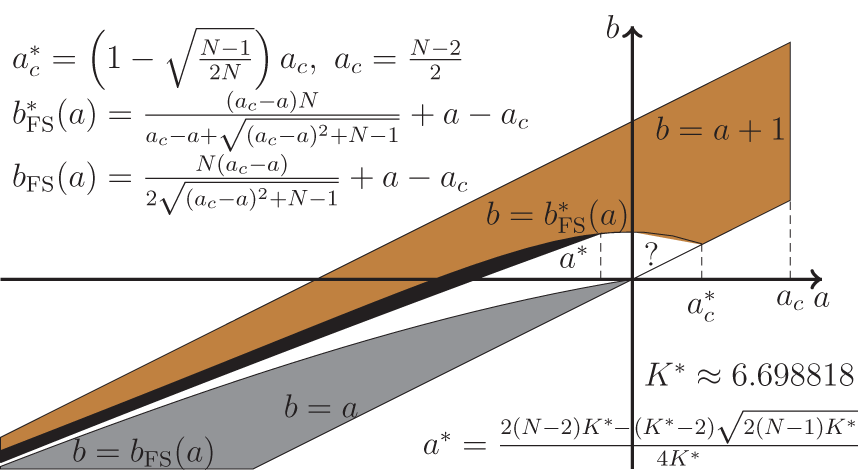
In the proof of lemma A.2, though the solution  $b^*(a)$ of (A.3) seems cannot be given explicitly, we can calculate some special (a, b) by using numerical simulation, see Table A.1. See also the schematic diagram in Figure A.2 for all
 $N\geq 2$.
Choices of  $b$ when
 $N=2$,
 $a \lt 0$ satisfying
 $b_{\mathrm{FS}}(a) \lt b \lt b^*_{\mathrm{FS}}(a)$.

Choices of (a, b) in brown and black regions for  $N\geq 2$. The brown region has been proved by Wei and Wu [Reference Wei and Wu26], and the black region is obtained in the present paper by using the approximation method. While, for the white region ‘?’, whether strict inequality (1.20) holds or not is still open.