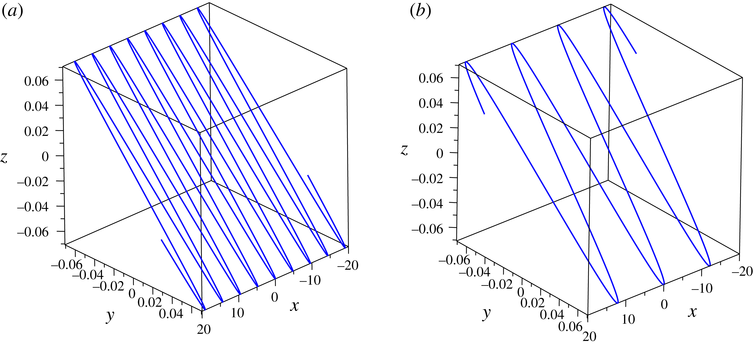
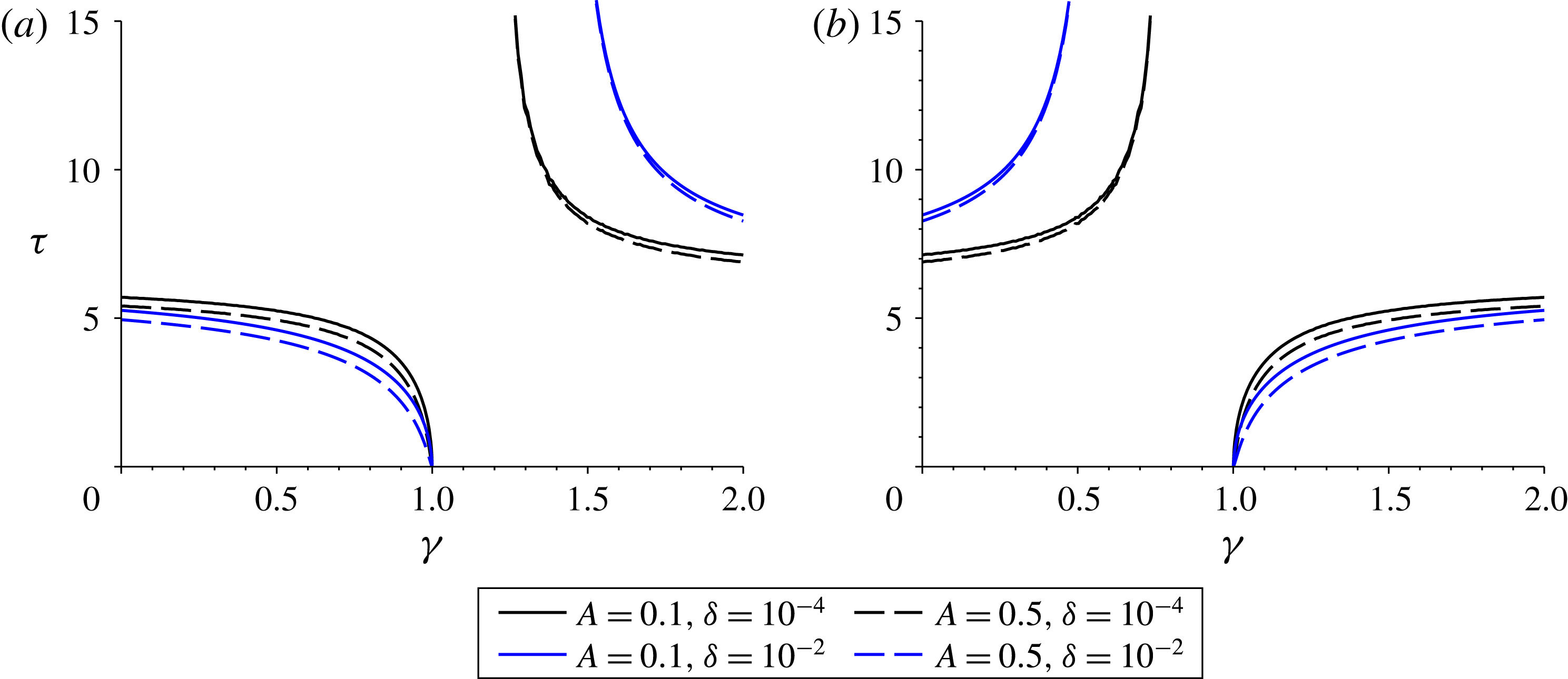
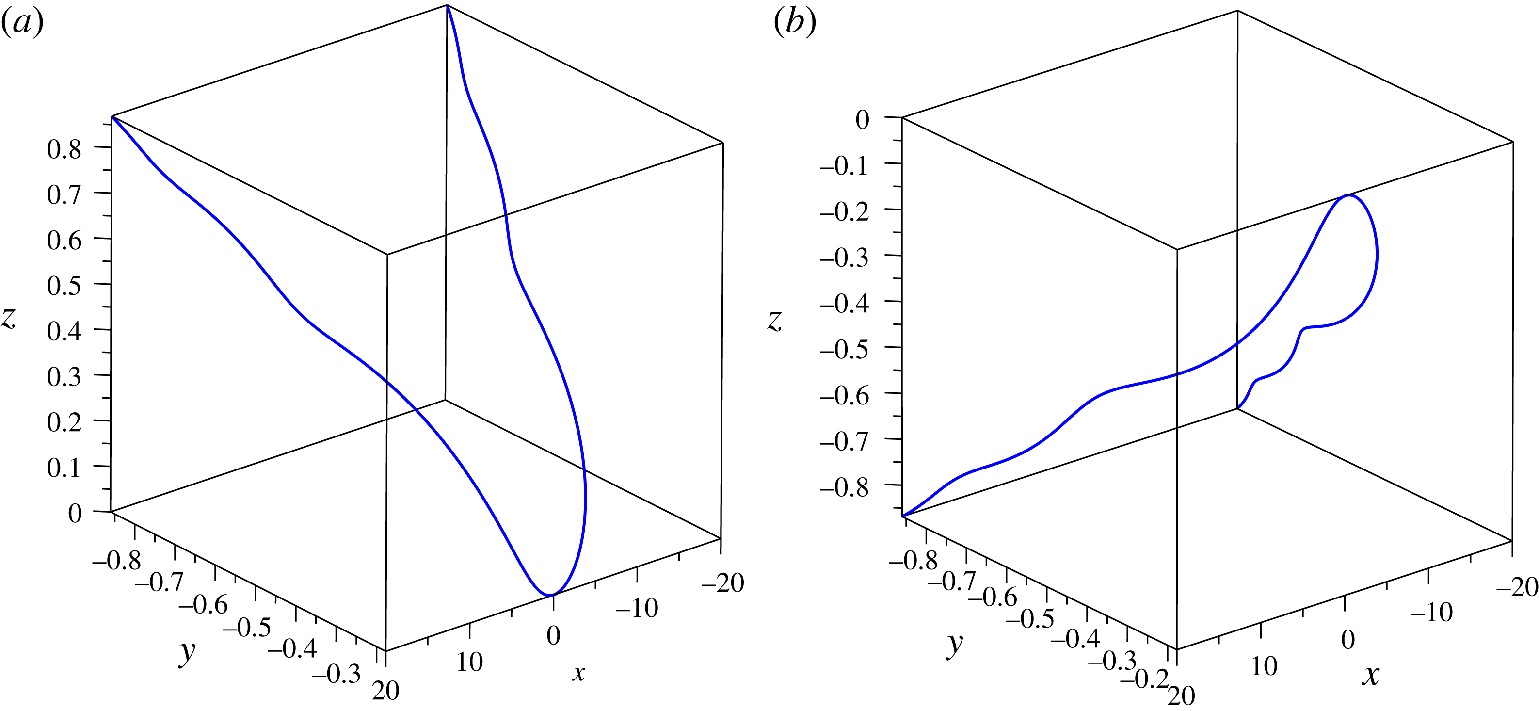
1 Introduction
The mathematical formulation of the self-induced motion of a vortex filament under no external forcing was rigorously examined by Da Rios (Reference Da Rios1906) and later rediscovered by Arms & Hama (Reference Arms and Hama1965). The natural framework for the discussion of vortex motion is the Biot–Savart law (Moore & Saffman Reference Moore and Saffman1972; Widnall Reference Widnall1972; Ricca Reference Ricca1991)
 $$\begin{eqnarray}\displaystyle \boldsymbol{r}_{t}=\frac{\unicode[STIX]{x1D705}}{4\unicode[STIX]{x03C0}}\int _{\mathbb{R}}\frac{[\boldsymbol{s}-\boldsymbol{r}]\times \text{d}\boldsymbol{s}}{|\boldsymbol{s}-\boldsymbol{r}|^{3}}, & & \displaystyle\end{eqnarray}$$
where
 $\boldsymbol{r}$
models the position of the filament at time
 $t$
,
 $\boldsymbol{s}$
is the variable of integration and the integral is taken over the length of the vortex filament. The quantity
 $\unicode[STIX]{x1D705}$
represents the strength of the vortex filament which is defined below.
This formulation is non-local and is sufficient to completely determine the motion of a single vortex filament. However, the implementation of this equation presents a considerable difficulty both analytically and numerically due to the well-known logarithmic singularity which occurs as
 $\boldsymbol{r}$
approaches
 $\boldsymbol{s}$
, a result of this being that the system is difficult to solve for all but the simplest vortex configurations. As a result of this difficulty, a variety of methods have been used to tackle this non-local equation and reduce it into a form which can be more easily examined.
Arms & Hama (Reference Arms and Hama1965) were able to derive a useful approximation for the induction effect of a smooth curved vortex on itself. This localised induction approximation (LIA) can be used to determine the behaviour of the filament due to local effects and provide a useful physical insight into the solutions of the system. This approximation is valid in the limiting case of a vortex filament of infinitesimal cross-section with negligible long distance effect. This formulation reduces the equation of motion to a system of partial differential equations (PDEs) which can be analysed effectively. The full Biot–Savart integral formulation can still be considered useful when the vortex filaments are tightly coiled, as shown in Newtonian fluids by Arms & Hama (Reference Arms and Hama1965) and quantum fluids by Van Gorder (Reference Van Gorder2015a ). Biot–Savart dynamics and approximations, in a purely hydrodynamic context, have been considered previously for helical vortex filaments (Widnall Reference Widnall1972; Van Gorder Reference Van Gorder2015b ), planar vortex filaments (Van Gorder Reference Van Gorder2015c ), and vortex filaments exhibiting self-similarity (Van Gorder Reference Van Gorder2016).
In the present work we are concerned with the motion of vortex filaments in plasmas and other electrically conducting fluids. The equations of motion for a vortex filament in the presence of both electric current and vorticity were first derived by Yatsuyanagi, Hatori & Kato (Reference Yatsuyanagi, Hatori and Kato1996). In this model, the electric current density and vorticity exist coaxially within the thin vortex filament, while neither exist outside the filament. The magnetic field and velocity are tangent to the surface of the filament. Filament solutions to this model are referred to as ‘vortex-current’ filaments. This model has applications to magnetohydrodynamic (MHD) flows, and was applied to tokamak devices (see Mukhovatov & Shafranov (Reference Mukhovatov and Shafranov1971), Miyamoto (Reference Miyamoto1980)), and resulting closed vortex-current filaments have been studied. This formulation utilises another approximation technique for the non-local Biot–Savart integrals known as the ‘cutoff’ approximation. The cutoff approximation regularises the Biot–Savart formulation by modifying the region of integration in such a way to avoid the singularity; further details can be found in Moore & Saffman (Reference Moore and Saffman1972), Siggia & Pumir (Reference Siggia and Pumir1985), Siggia (Reference Siggia1985). This formulation gives a result accurate to
 $O(\unicode[STIX]{x1D70C}^{-1})$
, where
 $\unicode[STIX]{x1D70C}$
is the radius of curvature of the filament curve at the point
 $\boldsymbol{r}$
on the curve. The resulting equations of motion contain a mixture of both hydrodynamic and MHD effects resulting in a rather complicated system and as such this formulation has not attracted considerable analytical attention in the literature.
Following on from the model of Yatsuyanagi et al. (Reference Yatsuyanagi, Hatori and Kato1996), there have been some works on the simulation of vortex-current filaments. Such work can be partitioned into deterministic models and statistical models. Regarding deterministic models, note that Yatsuyanagi, Hatori & Kato (Reference Yatsuyanagi, Hatori and Kato1998) have performed numerical simulations using a kind of reduced vortex-current model, with their primary focus being the examination of oscillations of vortex-current filament rings. Along similar lines, Yatsuyanagi et al. (Reference Yatsuyanagi, Ebisuzaki, Hatori and Kato2003) obtained numerical results via a ‘current-vortex’ method using an appropriate approximation to the Biot–Savart integrals present in such deterministic models. For more details on the numerical challenges and successful approaches for deterministic vortex-current problems, refer to Sheel, Yasuoka & Obi (Reference Sheel, Yasuoka and Obi2007). Simulations of deterministic chaotic reconnections in MHD were considered by Yatsuyanagi, Hatori & Kato (Reference Yatsuyanagi, Hatori and Kato2001) for related models of vortex-current filaments. Statistical models are also available for more complicated vortex-current filament dynamics in turbulent plasmas (Suzuki, Ito & Yoshida Reference Suzuki, Ito and Yoshida2003), with the benefit of such models being that they can simulate complex structures and flow regimes without solving complicated deterministic flow problems. In addition to the deterministic and statistical simulation results mentioned here, there have been theoretical results on Riemannian geometrical constraints for vortex magnetic filaments acting as dynamos in MHD flows are discussed by de Andrade (Reference de Andrade2006). However, theoretical studies on vortex-current filaments seem scarce, particularly concerning open vortex filaments. Therefore, we shall focus on various geometries of open filament solutions to the vortex-current filament model of Yatsuyanagi et al. (Reference Yatsuyanagi, Hatori and Kato1996), as such solutions have not attracted much attention thus far.
Regarding applications, the model of Yatsuyanagi et al. (Reference Yatsuyanagi, Hatori and Kato1996) can be used to study physical systems such as coronal loops. Yatsuyanagi et al. (Reference Yatsuyanagi, Hatori and Kato2001) studied chaotic reconnections within the model, in order to study the mechanism for fast magnetic reconnection, which is a fundamental process in solar flares (Shibata Reference Shibata1996). Furthermore, the model of Yatsuyanagi et al. (Reference Yatsuyanagi, Hatori and Kato1996) has been applied to the force balance analysis of the tokamak, with the previous work of Mukhovatov & Shafranov (Reference Mukhovatov and Shafranov1971) on the equilibrium of a toroidal plasma column in systems of the tokamak type recovered under restrictions on the geometry. More broadly, there have been recent experiments on vortex-current filaments. Soto et al. (Reference Soto, Pavez, Castillo, Veloso, Moreno and Auluck2014) provide experimental observations of filaments on a table-top plasma focus device using three techniques: framing photography of visible self-luminosity from the plasma, schlieren photography and interferometry. They found that there is a signature of the relaxed state of a Hall fluid, which has significant mass flow with equipartition between kinetic and magnetic energy, supporting the vortex filament description of the observed phenomenon. Alexandrova et al. (Reference Alexandrova, Mangeney, Maksimovic, Cornilleau-Wehrlin, Bosqued and André2006) suggested the observation of Alfvén vortex filaments in magnetosheath downstream of a quasi-perpendicular bow shock. Hence, there are indeed several phenomenon which might be described under a vortex-current filament model.
The aim of this work will be to examine the equation of motion for vortex filaments in the presence of MHD effects and glean some insight into the open vortex-current filament solutions of this system. The results obtained allow us to make comparisons between the hydrodynamic and MHD elements of the motion of vortex-current filaments. The remainder of this paper is organised as follows. In § 2 we review the vortex-current filament model of Yatsuyanagi et al. (Reference Yatsuyanagi, Hatori and Kato1996), and write the model in a way that describes the dynamics of a single isolated vortex-current filament, akin to formulations for the self-induced motion of an isolated vortex filament in an inviscid fluid. In § 3, we apply the model to the study of helical vortex-current filaments, in order to analytically obtain the equations governing the rotational and translational velocity of such vortex-current filaments. In § 4, we demonstrate the existence of planar vortex-current filaments under this model, and determine the properties of such solutions. In § 5, we demonstrate that self-similar vortex-current filaments also exist under the model of Yatsuyanagi et al. (Reference Yatsuyanagi, Hatori and Kato1996), and we describe the time evolution of such vortex-current filaments. We give concluding remarks in § 6.
2 MHD vortex-current filament model
In the MHD model set-up, the electric current density and vorticity exist coaxially inside the filament and neither of these quantities are defined outside of the filament. The magnetic field and velocity are tangential at the surface of the filament. Such a filament will be referred to as a vortex-current filament. Yatsuyanagi et al. (Reference Yatsuyanagi, Hatori and Kato1996) used a force balancing argument to obtain the following system of partial differential equations governing the motion of a vortex-current filament in an external magnetic field. In this section we shall review the derivations of Yatsuyanagi et al. (Reference Yatsuyanagi, Hatori and Kato1996) to put the model into context. We shall then be concerned with the solution of this model for several open vortex filament configurations.
The macroscopic equations of motion for a vortex filament without an electric current were developed by Moore & Saffman (Reference Moore and Saffman1972). The methods developed therein were followed by Yatsuyanagi et al. (Reference Yatsuyanagi, Hatori and Kato1996) to develop equations of motion of vortex-current filaments in magnetic fields. This was done by adapting the method of Moore & Saffman (Reference Moore and Saffman1972) to include both hydrodynamic and MHD effects. The approach is based on the idea that the equations of motion of the filament can be derived by balancing the forces acting on a small volume element
 $\unicode[STIX]{x1D6E5}$
of the vortex-current filament. The approach taken in Moore & Saffman (Reference Moore and Saffman1972) is then to integrate the macroscopic inviscid fluid equations over this volume element to gain information about the dynamics of the filaments. In this purely hydrodynamic model, the total force is built up of two constituent forces, namely an exterior force
 $\boldsymbol{F}_{E}$
acting on the curved surface of the filament and an interior force
 $\boldsymbol{F}_{I}$
acting on the edges of the filament. The exterior force includes the Kutta lift whereas the interior force is mainly due to axial flow. Yatsuyanagi et al. (Reference Yatsuyanagi, Hatori and Kato1996) extended this hydrodynamic model to include MHD effects – the approach is analogous to that taken by Moore & Saffman (Reference Moore and Saffman1972) whilst including additional force terms in
 $\boldsymbol{F}_{E}$
and
 $\boldsymbol{F}_{I}$
due to the presence of the electric current inside the filaments. They also include another force vector
 $\boldsymbol{G}$
which arises due to the presence of magnetic fields and is the volume integral of the Maxwell–Faraday equation.
As pointed out by Yatsuyanagi et al. (Reference Yatsuyanagi, Hatori and Kato1996), electromagnetics and hydrodynamics have many similarities. For instance, vorticity
 $\boldsymbol{\unicode[STIX]{x1D714}}$
is derived from velocity
 $\boldsymbol{u}$
in hydrodynamics as
 $\boldsymbol{\unicode[STIX]{x1D714}}=\unicode[STIX]{x1D735}\times \boldsymbol{u}$
while electric current density
 $\boldsymbol{j}$
is derived from a magnetic field
 $\boldsymbol{B}$
in electromagnetics as
 $\unicode[STIX]{x1D707}_{0}\boldsymbol{j}=\unicode[STIX]{x1D735}\times \boldsymbol{B}$
, where
 $\unicode[STIX]{x1D707}_{0}$
is the permeability constant (also referred to as the magnetic constant or the permeability of free space). Yatsuyanagi et al. (Reference Yatsuyanagi, Hatori and Kato1996) assume that the fluid is incompressible and the magnetic field solenoidal, hence
 $\unicode[STIX]{x1D735}\boldsymbol{\cdot }\boldsymbol{u}=0$
and
 $\unicode[STIX]{x1D735}\boldsymbol{\cdot }\boldsymbol{B}=0$
. In the model of Yatsuyanagi et al. (Reference Yatsuyanagi, Hatori and Kato1996), they assume electric current density and vorticity exist coaxially inside the vortex filament and neither exist outside of the filament.
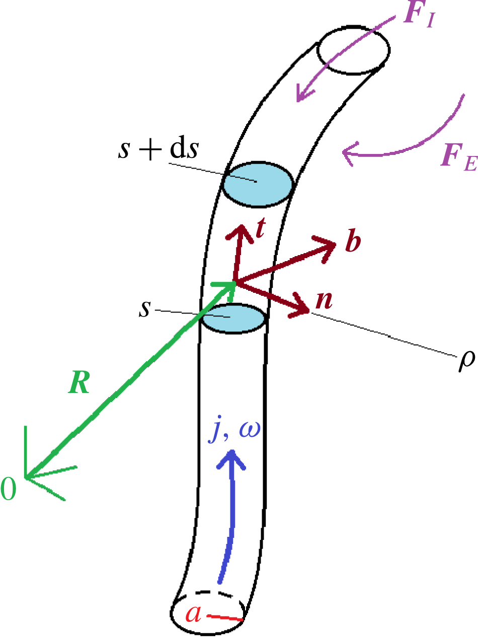
A point on the vortex filament can be denoted
 $\boldsymbol{R}(\unicode[STIX]{x1D709},t)$
with
 $\unicode[STIX]{x1D709}$
a parameter specifying position along the curve. The arclength
 $s=s(\unicode[STIX]{x1D709},t)$
can then be specified as
 $$\begin{eqnarray}\displaystyle \frac{\unicode[STIX]{x2202}s}{\unicode[STIX]{x2202}\unicode[STIX]{x1D709}}=\left|\frac{\unicode[STIX]{x2202}\boldsymbol{R}}{\unicode[STIX]{x2202}\unicode[STIX]{x1D709}}\right|. & & \displaystyle\end{eqnarray}$$
The form of the filament is then given by quantities
 $\boldsymbol{R}$
,
 $a$
,
 $\unicode[STIX]{x1D70C}$
; see the schematic diagram in figure 1. Here
 $a$
is the radius of the filament and
 $\unicode[STIX]{x1D70C}$
is the radius of curvature of the filament (which scales as the inverse of the scalar curvature of the filament curve). Generally,
 $a=a(\boldsymbol{R})$
and
 $\unicode[STIX]{x1D70C}=\unicode[STIX]{x1D70C}(\boldsymbol{R})$
. Inside the filament there exists a current,
 $J$
, defined by
 $J=\int \boldsymbol{j}\boldsymbol{\cdot }(\unicode[STIX]{x2202}\boldsymbol{R}/\unicode[STIX]{x2202}s)\,\text{d}A$
, and circulation,
 $\unicode[STIX]{x1D705}$
, defined by
 $\unicode[STIX]{x1D705}=\int \boldsymbol{\unicode[STIX]{x1D714}}\cdot (\unicode[STIX]{x2202}\boldsymbol{R}/\unicode[STIX]{x2202}s)\,\text{d}A$
. The filament velocity is given by
 $\unicode[STIX]{x2202}\boldsymbol{R}/\unicode[STIX]{x2202}t$
, and the filament moves due to self-induced velocity determined from the combination of electric current density and vorticity.
The geometry and notational conventions used for the open vortex-current filament. We denote by
 $\mathbf{0}$
the origin of the coordinate frame, and
 $\boldsymbol{R}$
a point on the vortex filament curve so that
 $\boldsymbol{R}(\unicode[STIX]{x1D701},t)$
traces out the filament in space at each time.
 $\boldsymbol{t}=\unicode[STIX]{x2202}\boldsymbol{R}/\unicode[STIX]{x2202}s$
denotes the tangent vector to the filament curve,
 $\boldsymbol{n}$
the normal vector and
 $\boldsymbol{b}$
the binormal vector.
 $j$
and
 $\unicode[STIX]{x1D714}$
denote the change and vorticity within the filament core, respectively, while
 $a$
is the radius of the filament and
 $\unicode[STIX]{x1D70C}$
is the radius of curvature of the filament.
 $\boldsymbol{F}_{E}$
and
 $\boldsymbol{F}_{I}$
are the external and internal forces, respectively.
 $s$
denotes arclength along the filament curve, and in order to derive expressions for the force Yatsuyanagi et al. (Reference Yatsuyanagi, Hatori and Kato1996) considered volume elements
 $\unicode[STIX]{x1D6E5}$
within the filaments bounded by planes
 $E_{1}$
and
 $E_{2}$
located at
 $s$
and
 $s+\text{d}s$
and a curved surface
 $C$
formed by the intermediate filament boundary between
 $E_{1}$
and
 $E_{2}$
.

In order to derive
 $\unicode[STIX]{x2202}\boldsymbol{R}/\unicode[STIX]{x2202}t$
and to hence determine the equations governing the motion of a vortex-current filament, Yatsuyanagi et al. (Reference Yatsuyanagi, Hatori and Kato1996) start with the ideal MHD equations, which read
 $$\begin{eqnarray}\displaystyle & \displaystyle \frac{\unicode[STIX]{x2202}\boldsymbol{u}}{\unicode[STIX]{x2202}t}+(\boldsymbol{u}\boldsymbol{\cdot }\unicode[STIX]{x1D735})\boldsymbol{u}=\boldsymbol{j}\times \boldsymbol{B}-\unicode[STIX]{x1D735}p, & \displaystyle\end{eqnarray}$$
 $$\begin{eqnarray}\displaystyle & \displaystyle \unicode[STIX]{x1D735}\boldsymbol{\cdot }\boldsymbol{u}=0, & \displaystyle\end{eqnarray}$$
 $$\begin{eqnarray}\displaystyle & \displaystyle \unicode[STIX]{x1D735}\times \boldsymbol{u}=\boldsymbol{\unicode[STIX]{x1D714}}, & \displaystyle\end{eqnarray}$$
 $$\begin{eqnarray}\displaystyle & \displaystyle \frac{\unicode[STIX]{x2202}\boldsymbol{B}}{\unicode[STIX]{x2202}t}=-\unicode[STIX]{x1D735}\times \boldsymbol{E}, & \displaystyle\end{eqnarray}$$
 $$\begin{eqnarray}\displaystyle & \displaystyle \unicode[STIX]{x1D735}\boldsymbol{\cdot }\boldsymbol{B}=0, & \displaystyle\end{eqnarray}$$
 $$\begin{eqnarray}\displaystyle & \displaystyle \unicode[STIX]{x1D735}\times \boldsymbol{B}=\unicode[STIX]{x1D707}_{0}\,\,\boldsymbol{j}, & \displaystyle\end{eqnarray}$$
 $$\begin{eqnarray}\displaystyle & \displaystyle \boldsymbol{E}+\boldsymbol{u}\times \boldsymbol{B}=0, & \displaystyle\end{eqnarray}$$
 $$\begin{eqnarray}\displaystyle & \displaystyle \unicode[STIX]{x1D735}\boldsymbol{\cdot }\boldsymbol{D}=0, & \displaystyle\end{eqnarray}$$
with mass density normalised to one (since the fluid is incompressible). Here,
 $\boldsymbol{B}$
is the magnetic field,
 $\boldsymbol{E}$
is the electric field,
 $p$
is pressure, and
 $\unicode[STIX]{x1D707}_{0}$
is the permeability constant. Yatsuyanagi et al. (Reference Yatsuyanagi, Hatori and Kato1996) consider an element
 $\unicode[STIX]{x1D6E5}$
of the vortex-current filament with length
 $\text{d}s$
bounded by a curved surface
 $C$
and plane ends
 $E_{1}$
at
 $s$
and
 $E_{2}$
at
 $s+\text{d}s$
, with the plane ends normal to
 $s$
. It was shown that (2.2) and (2.5) integrate to
 $$\begin{eqnarray}\displaystyle & & \displaystyle \frac{\unicode[STIX]{x2202}}{\unicode[STIX]{x2202}t}\int _{\unicode[STIX]{x1D6E5}}\boldsymbol{u}\,\text{d}V+\int _{E_{1}+E_{2}}\left\{\left(p+\frac{|\boldsymbol{B}|^{2}}{2\unicode[STIX]{x1D707}_{0}}\right)\boldsymbol{l}+(\boldsymbol{u}^{rel}\boldsymbol{\cdot }\boldsymbol{l})\boldsymbol{u}-\frac{1}{\unicode[STIX]{x1D707}_{0}}(\boldsymbol{B}\boldsymbol{\cdot }\boldsymbol{l})\boldsymbol{B}\right\}\,\text{d}A\nonumber\\ \displaystyle & & \displaystyle \qquad +\int _{C}\left(p+\frac{|\boldsymbol{B}|^{2}}{2\unicode[STIX]{x1D707}_{0}}\right)\boldsymbol{l}\,\text{d}A=0\end{eqnarray}$$
and
 $$\begin{eqnarray}\displaystyle \frac{\unicode[STIX]{x2202}}{\unicode[STIX]{x2202}t}\int _{\unicode[STIX]{x1D6E5}}\boldsymbol{B}\,\text{d}V+\int _{E_{1}+E_{2}}\{(\boldsymbol{u}^{rel}\boldsymbol{\cdot }\boldsymbol{l})\boldsymbol{B}-(\boldsymbol{B}\boldsymbol{\cdot }\boldsymbol{l})\boldsymbol{u}\}\,\text{d}A=0, & & \displaystyle\end{eqnarray}$$
respectively, where
 $\text{d}A$
denotes a surface area element. Here
 $\boldsymbol{u}$
is the fluid velocity while
 $\boldsymbol{u}^{rel}$
is the fluid velocity relative to the element
 $\unicode[STIX]{x1D6E5}$
. The outward normal to the curved surface is denoted by
 $\boldsymbol{l}$
. Then, Yatsuyanagi et al. (Reference Yatsuyanagi, Hatori and Kato1996) write (2.10)–(2.11) as
 $\boldsymbol{F}_{E}+\boldsymbol{F}_{I}=\mathbf{0}$
and
 $\boldsymbol{G}=\mathbf{0}$
, respectively, where
 $$\begin{eqnarray}\displaystyle & \displaystyle -\text{d}s\boldsymbol{F}_{E}=\int _{C}\left(p+\frac{|\boldsymbol{B}|^{2}}{2\unicode[STIX]{x1D707}_{0}}\right)\boldsymbol{l}\,\text{d}A, & \displaystyle\end{eqnarray}$$
 $$\begin{eqnarray}\displaystyle & \displaystyle -\text{d}s\boldsymbol{F}_{I}=\frac{\unicode[STIX]{x2202}}{\unicode[STIX]{x2202}t}\int _{\unicode[STIX]{x1D6E5}}\boldsymbol{u}\,\text{d}V+\int _{E_{1}+E_{2}}\left\{\left(p+\frac{|\boldsymbol{B}|^{2}}{2\unicode[STIX]{x1D707}_{0}}\right)\boldsymbol{l}+(\boldsymbol{u}^{rel}\boldsymbol{\cdot }\boldsymbol{l})\boldsymbol{u}-\frac{1}{\unicode[STIX]{x1D707}_{0}}(\boldsymbol{B}\boldsymbol{\cdot }\boldsymbol{l})\boldsymbol{B}\right\}\,\text{d}A, & \displaystyle\end{eqnarray}$$
and
 $$\begin{eqnarray}\displaystyle -\text{d}s\boldsymbol{G}=\frac{\unicode[STIX]{x2202}}{\unicode[STIX]{x2202}t}\int _{\unicode[STIX]{x1D6E5}}\boldsymbol{B}\,\text{d}V+\int _{E_{1}+E_{2}}\{(\boldsymbol{u}^{rel}\boldsymbol{\cdot }\boldsymbol{l})\boldsymbol{B}-(\boldsymbol{B}\boldsymbol{\cdot }\boldsymbol{l})\boldsymbol{u}\}\,\text{d}A. & & \displaystyle\end{eqnarray}$$
 $\boldsymbol{F}_{E}$
is the exterior force per unit length exerted by the fluid outside the filament on the curved surface
 $C$
,
 $\boldsymbol{F}_{I}$
is the interior force per unit length exerted on the curved by the fluid inside the filament and
 $\boldsymbol{G}$
is the volume integral of Faraday’s equation. Yatsuyanagi et al. (Reference Yatsuyanagi, Hatori and Kato1996) then proceed to calculate each of these force terms in order to obtain an expression for
 $\unicode[STIX]{x2202}\boldsymbol{R}/\unicode[STIX]{x2202}t$
.
Much of Yatsuyanagi et al. (Reference Yatsuyanagi, Hatori and Kato1996) is devoted to deriving expressions for these forces. We shall therefore omit the details, and give the forces. Partitioning the fields
 $\boldsymbol{B}$
and
 $\boldsymbol{u}$
into internal (subscript
 $I$
) and external (subscript
 $E$
) components, Yatsuyanagi et al. (Reference Yatsuyanagi, Hatori and Kato1996) find
 $$\begin{eqnarray}\displaystyle \boldsymbol{F}_{E} & = & \displaystyle -J(\boldsymbol{B}_{E}(\boldsymbol{R})+\boldsymbol{B}_{I}(\boldsymbol{R}))\times \frac{\unicode[STIX]{x2202}\boldsymbol{R}}{\unicode[STIX]{x2202}s}+\unicode[STIX]{x1D705}\left(\boldsymbol{u}_{E}(\boldsymbol{R})+\boldsymbol{u}_{I}(\boldsymbol{R})-\frac{\unicode[STIX]{x2202}\boldsymbol{R}}{\unicode[STIX]{x2202}t}\right)\times \frac{\unicode[STIX]{x2202}\boldsymbol{R}}{\unicode[STIX]{x2202}s}\nonumber\\ \displaystyle & & \displaystyle -\,\frac{\unicode[STIX]{x1D707}_{0}J^{2}}{4\unicode[STIX]{x03C0}\unicode[STIX]{x1D70C}}\left(\ln \frac{8\unicode[STIX]{x1D70C}}{a_{j0}}-\frac{1}{2}\right)\boldsymbol{n}+\frac{\unicode[STIX]{x1D705}^{2}}{4\unicode[STIX]{x03C0}\unicode[STIX]{x1D70C}}\left(\ln \frac{8\unicode[STIX]{x1D70C}}{a_{\unicode[STIX]{x1D714}0}}-\frac{1}{2}\right)\boldsymbol{n}\nonumber\\ \displaystyle & & \displaystyle +\,\frac{\unicode[STIX]{x1D707}_{0}J^{2}}{8\unicode[STIX]{x03C0}a_{j0}^{2}}\frac{\unicode[STIX]{x2202}a_{j0}^{2}}{\unicode[STIX]{x2202}s}\frac{\unicode[STIX]{x2202}\boldsymbol{R}}{\unicode[STIX]{x2202}s}-\frac{\unicode[STIX]{x1D705}^{2}}{8\unicode[STIX]{x03C0}a_{\unicode[STIX]{x1D714}0}^{2}}\frac{\unicode[STIX]{x2202}a_{\unicode[STIX]{x1D714}0}^{2}}{\unicode[STIX]{x2202}s}\frac{\unicode[STIX]{x2202}\boldsymbol{R}}{\unicode[STIX]{x2202}s}\frac{\unicode[STIX]{x2202}\boldsymbol{R}}{\unicode[STIX]{x2202}s}+\frac{\unicode[STIX]{x1D707}_{0}J^{2}}{8\unicode[STIX]{x03C0}\unicode[STIX]{x1D70C}}\boldsymbol{n}-\frac{\unicode[STIX]{x1D705}^{2}}{8\unicode[STIX]{x03C0}\unicode[STIX]{x1D70C}}\boldsymbol{n},\end{eqnarray}$$
where
 $\boldsymbol{n}$
is the normal vector to
 $\boldsymbol{R}$
;
 $\unicode[STIX]{x2202}^{2}\boldsymbol{R}/\unicode[STIX]{x2202}s^{2}$
. Similarly, Yatsuyanagi et al. (Reference Yatsuyanagi, Hatori and Kato1996) derive the expression
 $$\begin{eqnarray}\displaystyle \boldsymbol{F}_{I} & = & \displaystyle \frac{\unicode[STIX]{x03C0}}{2}\frac{\unicode[STIX]{x2202}}{\unicode[STIX]{x2202}s}\left\{a_{\unicode[STIX]{x1D714}0}^{2}\overline{v_{0}^{2}}\frac{\unicode[STIX]{x2202}\boldsymbol{R}}{\unicode[STIX]{x2202}s}-\frac{1}{\unicode[STIX]{x1D707}_{0}}a_{j0}^{2}\overline{B_{0}^{2}}\frac{\unicode[STIX]{x2202}\boldsymbol{R}}{\unicode[STIX]{x2202}s}\right\}+\frac{1}{8\unicode[STIX]{x03C0}}(\unicode[STIX]{x1D705}^{2}-\unicode[STIX]{x1D707}_{0}J^{2})\frac{\boldsymbol{n}}{\unicode[STIX]{x1D70C}}\nonumber\\ \displaystyle & & \displaystyle +\,\unicode[STIX]{x03C0}\frac{\unicode[STIX]{x2202}}{\unicode[STIX]{x2202}s}\left\{\frac{1}{\unicode[STIX]{x1D707}_{0}}a_{j0}^{2}\overline{B_{0}^{2}}\frac{\unicode[STIX]{x2202}\boldsymbol{R}}{\unicode[STIX]{x2202}s}-a_{\unicode[STIX]{x1D714}0}^{2}\overline{w^{2}}\frac{\unicode[STIX]{x2202}\boldsymbol{R}}{\unicode[STIX]{x2202}s}-a_{\unicode[STIX]{x1D714}0}^{2}\overline{w}\frac{\unicode[STIX]{x2202}\boldsymbol{R}}{\unicode[STIX]{x2202}t}\right\}\nonumber\\ \displaystyle & & \displaystyle +\,\frac{\unicode[STIX]{x2202}}{\unicode[STIX]{x2202}s}\left\{\frac{a_{j0}^{2}}{\unicode[STIX]{x1D70C}}\unicode[STIX]{x1D706}_{1}J\overline{B_{\Vert }}\boldsymbol{b}-\frac{a_{\unicode[STIX]{x1D714}0}^{2}}{\unicode[STIX]{x1D70C}}\unicode[STIX]{x1D706}_{2}\unicode[STIX]{x1D705}\overline{w}\boldsymbol{b}\right\}\nonumber\\ \displaystyle & & \displaystyle -\,\unicode[STIX]{x03C0}\frac{\unicode[STIX]{x2202}}{\unicode[STIX]{x2202}t}\left\{a_{\unicode[STIX]{x1D714}0}^{2}\overline{w}\frac{\unicode[STIX]{x2202}\boldsymbol{R}}{\unicode[STIX]{x2202}s}+a_{\unicode[STIX]{x1D714}0}^{2}\overline{w}\frac{\unicode[STIX]{x2202}\boldsymbol{R}}{\unicode[STIX]{x2202}s}\frac{\unicode[STIX]{x2202}}{\unicode[STIX]{x2202}t}\left(\ln \left(\frac{\unicode[STIX]{x2202}s}{\unicode[STIX]{x2202}\unicode[STIX]{x1D709}}\right)\right)\right\}.\end{eqnarray}$$
Regarding notation, the resultant magnetic field is decomposed as
 $\boldsymbol{B}_{E}$
, the magnetic field due to external sources and
 $\boldsymbol{B}_{I}$
, the magnetic field due to the filament itself. Similarly the velocity field is decomposed as
 $\boldsymbol{u}_{E}$
, the velocity field due to external sources and
 $\boldsymbol{u}_{I}$
, the velocity field due to the filament itself (see Moore & Saffman (Reference Moore and Saffman1972)).
 $\boldsymbol{b}=(\unicode[STIX]{x2202}\boldsymbol{R}/\unicode[STIX]{x2202}s)\times \boldsymbol{n}$
is the binormal vector to the filament. The radius of curvature and the radius of the filament are denoted by
 $\unicode[STIX]{x1D70C}=\unicode[STIX]{x1D70C}(\boldsymbol{r})$
and
 $a=a(\boldsymbol{r})$
respectively. The variable
 $a_{0}$
is the leading term in the Taylor expansion of the radius
 $a$
in powers of the radius of curvature
 $\unicode[STIX]{x1D70C}$
. Subscripts
 $j$
and
 $\unicode[STIX]{x1D714}$
refer to the extent of the current and vorticity within the filament; for practical purposes these will often be set to
 $a_{j0}=a_{\unicode[STIX]{x1D714}0}=a_{0}$
. The constant
 $\unicode[STIX]{x1D707}_{0}$
is the permeability of the fluid. The
 $B_{\Vert }$
and
 $w$
are the components of the magnetic field and velocity inside the filament which are parallel to the vector
 $\boldsymbol{s},$
whereas
 $B_{0}$
and
 $v_{0}$
are the leading-order azimuthal components of the magnetic field and velocity respectively. Here the notation
 $\bar{A}$
denotes the mean value of
 $A$
over a cross-section of the filament.
Regarding the expression for
 $\boldsymbol{G}$
, it is shown that
 $\boldsymbol{G}=O(\unicode[STIX]{x1D70C}^{-2})$
, hence this term is neglected. Further, decomposing
 $\boldsymbol{F}_{\bot }+\boldsymbol{F}_{\Vert }$
, Yatsuyanagi et al. (Reference Yatsuyanagi, Hatori and Kato1996) found that
 $\boldsymbol{F}_{\Vert }=O(\unicode[STIX]{x1D70C}^{-2})$
. Retaining only terms up to
 $O(\unicode[STIX]{x1D70C}^{-1})$
, the equation
 $\boldsymbol{F}_{\bot }=\mathbf{0}$
is obtained. Multiplying this by
 $\unicode[STIX]{x2202}\boldsymbol{R}/\unicode[STIX]{x2202}s$
, Yatsuyanagi et al. (Reference Yatsuyanagi, Ebisuzaki, Hatori and Kato2003) obtain the equation
 $$\begin{eqnarray}\displaystyle \left(\frac{\unicode[STIX]{x2202}\boldsymbol{R}}{\unicode[STIX]{x2202}t}\right)_{\bot } & = & \displaystyle -\frac{J}{\unicode[STIX]{x1D705}}[(\boldsymbol{B}_{\boldsymbol{E}})_{\bot }+(\boldsymbol{B}_{\boldsymbol{I}})_{\bot }]+(\boldsymbol{u}_{\boldsymbol{E}})_{\bot }+(\boldsymbol{u}_{\boldsymbol{I}})_{\bot }\nonumber\\ \displaystyle & & \displaystyle -\,\frac{\unicode[STIX]{x1D707}_{0}J^{2}\boldsymbol{b}}{4\unicode[STIX]{x03C0}\unicode[STIX]{x1D70C}\unicode[STIX]{x1D705}}\left(\ln \left(\frac{8\unicode[STIX]{x1D70C}}{a_{j0}}-\frac{1}{2}\right)\right)-\frac{\unicode[STIX]{x03C0}a_{0j}^{2}\boldsymbol{b}}{\unicode[STIX]{x1D70C}\unicode[STIX]{x1D705}}\left(\frac{\bar{B_{0}^{2}}}{2\unicode[STIX]{x1D707}_{0}}-\frac{\bar{B_{\Vert }^{2}}}{\unicode[STIX]{x1D707}_{0}}\right)\nonumber\\ \displaystyle & & \displaystyle +\,\frac{\unicode[STIX]{x1D705}\boldsymbol{b}}{4\unicode[STIX]{x03C0}\unicode[STIX]{x1D70C}}\left(\ln \left(\frac{8\unicode[STIX]{x1D70C}}{a_{\unicode[STIX]{x1D714}0}}-\frac{1}{2}\right)\right)+\frac{\unicode[STIX]{x03C0}a_{\unicode[STIX]{x1D714}0}^{2}\boldsymbol{b}}{\unicode[STIX]{x1D70C}\unicode[STIX]{x1D705}}\left(\bar{\frac{v_{0}^{2}}{2}}-\bar{w^{2}}\right)+O(\unicode[STIX]{x1D70C}^{-2}).\end{eqnarray}$$
The filament moves with a self-induced velocity which is determined by the electric current density and vorticity. The velocity of the filament is also influenced by any changes in the external velocity field and magnetic field which may be present initially or generated by other filaments. This current work aims to describe the motion of a single isolated vortex filament and it hence follows that
 $\boldsymbol{B}_{E}=\boldsymbol{u}_{E}=\mathbf{0}$
. This means that the current and vorticity are confined to within the filament core, and are not influenced by outside effects. It can then be shown (see Yatsuyanagi et al. (Reference Yatsuyanagi, Hatori and Kato1996), equation (6.10)) that the model (2.17) reduces to
 $$\begin{eqnarray}\displaystyle \left(\frac{\unicode[STIX]{x2202}\boldsymbol{r}}{\unicode[STIX]{x2202}t}\right)_{\bot }=\frac{\unicode[STIX]{x1D6FE}_{M}}{2}\int \frac{[\boldsymbol{r}-\boldsymbol{r}]\times \text{d}\boldsymbol{s}}{[|\boldsymbol{r}-\boldsymbol{s}|^{2}+\unicode[STIX]{x1D6FC}^{2}]^{3/2}}-\frac{\unicode[STIX]{x1D6FE}_{H}}{2}\int \frac{[\boldsymbol{r}-\boldsymbol{s}]\times \text{d}\boldsymbol{s}}{[|\boldsymbol{r}-\boldsymbol{s}|^{2}+\unicode[STIX]{x1D6FD}^{2}]^{3/2}}, & & \displaystyle\end{eqnarray}$$
where
 $\unicode[STIX]{x1D6FC}$
and
 $\unicode[STIX]{x1D6FD}$
are the ‘cutoff’ parameters which are defined to satisfy the following conditions:
 $$\begin{eqnarray}\displaystyle & \displaystyle -\frac{\unicode[STIX]{x1D707}_{0}J^{2}}{4\unicode[STIX]{x03C0}\unicode[STIX]{x1D70C}\unicode[STIX]{x1D705}}\left(\ln \left(\frac{8\unicode[STIX]{x1D70C}}{a_{j0}}-\frac{1}{2}\right)\right)-\frac{\unicode[STIX]{x03C0}a_{0j}^{2}}{\unicode[STIX]{x1D70C}\unicode[STIX]{x1D705}}\left(\frac{\bar{B_{0}^{2}}}{2\unicode[STIX]{x1D707}_{0}}-\frac{\bar{B_{\Vert }^{2}}}{\unicode[STIX]{x1D707}_{0}}\right)=-\frac{\unicode[STIX]{x1D707}_{0}J^{2}}{4\unicode[STIX]{x03C0}\unicode[STIX]{x1D70C}\unicode[STIX]{x1D705}}\left(\ln \left(\frac{8\unicode[STIX]{x1D70C}}{\unicode[STIX]{x1D6FC}}\right)-1\right), & \displaystyle\end{eqnarray}$$
 $$\begin{eqnarray}\displaystyle & \displaystyle \frac{\unicode[STIX]{x1D705}}{4\unicode[STIX]{x03C0}\unicode[STIX]{x1D70C}}\left(\ln \left(\frac{8\unicode[STIX]{x1D70C}}{a_{\unicode[STIX]{x1D714}0}}-\frac{1}{2}\right)\right)+\frac{\unicode[STIX]{x03C0}a_{\unicode[STIX]{x1D714}0}^{2}}{\unicode[STIX]{x1D70C}\unicode[STIX]{x1D705}}\left(\bar{\frac{v_{0}^{2}}{2}}-\bar{w^{2}}\right)=\frac{\unicode[STIX]{x1D705}}{4\unicode[STIX]{x03C0}\unicode[STIX]{x1D70C}}\left(\ln \left(\frac{8\unicode[STIX]{x1D70C}}{\unicode[STIX]{x1D6FD}}\right)-1\right). & \displaystyle\end{eqnarray}$$
Here we have also defined the parameters
 $$\begin{eqnarray}\displaystyle \unicode[STIX]{x1D6FE}_{M}=\frac{\unicode[STIX]{x1D707}_{0}J^{2}}{2\unicode[STIX]{x03C0}\unicode[STIX]{x1D705}},\quad \unicode[STIX]{x1D6FE}_{H}=\frac{\unicode[STIX]{x1D705}}{2\unicode[STIX]{x03C0}}. & & \displaystyle\end{eqnarray}$$
These parameters are of particular interest here as they control how the vortex filaments will be affected by the presence of MHD terms. More specifically, the parameter
 $\unicode[STIX]{x1D6FE}_{H}$
only ‘feels’ the hydrodynamic effects whereas the parameter
 $\unicode[STIX]{x1D6FE}_{M}$
‘feels’ the MHD effects through its dependence on the term
 $J^{2}$
. If
 $\unicode[STIX]{x1D6FE}_{M}=0$
, then note that (2.18) will reduce to (1.1). By investigating how the solutions change as the ratio of these parameters is varied, we can hope to glean insight as to how the presence of the magnetic field affects the filament dynamics. For simplicity, and to remove the effect of the circulation on the results, we will scale time by
 $\unicode[STIX]{x1D705}/4\unicode[STIX]{x03C0}$
hence the only parameter of interest will be
 $$\begin{eqnarray}\displaystyle \unicode[STIX]{x1D6FE}=\frac{\unicode[STIX]{x1D707}_{0}J^{2}}{\unicode[STIX]{x1D705}^{2}}, & & \displaystyle\end{eqnarray}$$
where we note that this parameter is necessarily non-negative. This gives the equation
 $$\begin{eqnarray}\displaystyle \left(\frac{\unicode[STIX]{x2202}\boldsymbol{r}}{\unicode[STIX]{x2202}t}\right)_{\bot }=\unicode[STIX]{x1D6FE}\int \frac{[\boldsymbol{r}-\boldsymbol{r}]\times \text{d}\boldsymbol{s}}{[|\boldsymbol{r}-\boldsymbol{s}|^{2}+\unicode[STIX]{x1D6FC}^{2}]^{3/2}}-\int \frac{[\boldsymbol{r}-\boldsymbol{s}]\times \text{d}\boldsymbol{s}}{[|\boldsymbol{r}-\boldsymbol{s}|^{2}+\unicode[STIX]{x1D6FD}^{2}]^{3/2}}, & & \displaystyle\end{eqnarray}$$
the solution of which shall be the focus of this paper. When the hydrodynamic and MHD effects perfectly balance,
 $\unicode[STIX]{x1D6FE}=1$
.
3 Helical vortex-current filaments
A helical vortex filament is perhaps one of the most standard solutions studied analytically under either local induction approximation (LIA) or Biot–Savart dynamics in the hydrodynamic case, and is a natural solution to consider for a vortex-current filament. Regarding helical filaments, the ‘cutoff’ method based on the oscillating vortex ring has been employed to the study of helical vortex filaments (Widnall Reference Widnall1972). An analysis of the approach was conducted by Moore & Saffman (Reference Moore and Saffman1972). Using the ‘cutoff’ method Ricca (Reference Ricca1994) obtained analytical results in the small helix diameter and large torsion limit, and demonstrated that torsion strongly influences the motion of helical filaments. Results have been given in the small pitch (large wavenumbers) and small-amplitude regime (Widnall Reference Widnall1972; Ricca Reference Ricca1994), while Ricca (Reference Ricca1994) also gives an analytic result for the infinite-torsion case, valid when the pitch is small (wavenumber is large). Additional studies on the ‘cutoff’ method (Boersma & Wood Reference Boersma and Wood1999) have improved these results. Analytical results are common under the LIA (Zhou Reference Zhou1997), which is much simpler to solve in the helical case (Kida Reference Kida1981; Sonin Reference Sonin2012). Results on the helical filament which use the LIA to regularise the core region (rather than using the cutoff method) and also keep the Biot–Savart integral ‘tails’ were presented in Van Gorder (Reference Van Gorder2015b ), and were in good general agreement with the aforementioned cutoff method results.
3.1 Derivation of the rotational and translational velocities for a helical vortex-current filament
Here we shall consider the cutoff method to obtain helical filament solutions to (2.23). For simplicity, we align our helical filament along the
 $z$
coordinate axis as in Van Gorder (Reference Van Gorder2015b
). Hence a suitable representation of
 $\boldsymbol{r}$
is
 $$\begin{eqnarray}\displaystyle \boldsymbol{r}(x,t)=(x+Vt,A\cos (kx-\unicode[STIX]{x1D714}t+x_{0}),A\sin (kx-\unicode[STIX]{x1D714}t+x_{0})). & & \displaystyle\end{eqnarray}$$
The motion of the vortex-current filament is then governed by the values of
 $V$
(the transverse velocity of a helical wave along the line filament
 $A=0$
) and the rotational velocity
 $\unicode[STIX]{x1D714}$
. Substituting this representation into the model (2.23), the following system is obtained:
 $$\begin{eqnarray}\displaystyle V=\frac{\unicode[STIX]{x1D6FE}A^{2}k}{2}\int _{\mathbb{R}}\frac{\cos (k[x-S])-1}{F(x-S,\unicode[STIX]{x1D6FC})}\text{d}s-\frac{A^{2}k}{2}\int _{\mathbb{R}}\frac{\cos (k[x-S])-1}{F(x-S,\unicode[STIX]{x1D6FD})}\text{d}s, & & \displaystyle\end{eqnarray}$$
 $$\begin{eqnarray}\displaystyle & & \displaystyle A\unicode[STIX]{x1D714}\sin (kx-\unicode[STIX]{x1D714}t+x_{0})\nonumber\\ \displaystyle & & \displaystyle \quad =\frac{\unicode[STIX]{x1D6FE}A}{2}\int _{\mathbb{R}}\frac{\sin (kx-\unicode[STIX]{x1D714}t+x_{0})-\sin (kS-\unicode[STIX]{x1D714}t+x_{0})-k(x-S)\cos (kS-\unicode[STIX]{x1D714}t+x_{0})}{F(x-S,\unicode[STIX]{x1D6FC})}\,\text{d}s\nonumber\\ \displaystyle & & \displaystyle \qquad -\,\frac{A}{2}\int _{\mathbb{R}}\frac{\sin (kx-\unicode[STIX]{x1D714}t+x_{0})-\sin (kS-\unicode[STIX]{x1D714}t+x_{0})-k(x-S)\cos (kS-\unicode[STIX]{x1D714}t+x_{0})}{F(x-S,\unicode[STIX]{x1D6FD})}\,\text{d}s,\end{eqnarray}$$
 $$\begin{eqnarray}\displaystyle & & \displaystyle -A\unicode[STIX]{x1D714}\cos (kx-\unicode[STIX]{x1D714}t+x_{0})\nonumber\\ \displaystyle & & \displaystyle \quad =\frac{\unicode[STIX]{x1D6FE}A}{2}\int _{\mathbb{R}}\frac{-\cos (kx-\unicode[STIX]{x1D714}t+x_{0})+\cos (kS-\unicode[STIX]{x1D714}t+x_{0})-k(x-S)\sin (kS-\unicode[STIX]{x1D714}t+x_{0})}{F(x-S,\unicode[STIX]{x1D6FC})}\,\text{d}s\nonumber\\ \displaystyle & & \displaystyle \qquad -\,\frac{A}{2}\int _{\mathbb{R}}\frac{-\cos (kx-\unicode[STIX]{x1D714}t+x_{0})+\cos (kS-\unicode[STIX]{x1D714}t+x_{0})-k(x-S)\sin (kS-\unicode[STIX]{x1D714}t+x_{0})}{F(x-S,\unicode[STIX]{x1D6FD})}\,\text{d}s,\nonumber\\ \displaystyle & & \displaystyle\end{eqnarray}$$
where we have used
 $$\begin{eqnarray}\displaystyle F(p,q)=\{p^{2}+2A^{2}(1-\cos (kp))+q^{2}\}^{3/2}. & & \displaystyle\end{eqnarray}$$
Following Van Gorder (Reference Van Gorder2015b ), we take i times equation (3.3) and subtract equation (3.4) to obtain
 $$\begin{eqnarray}\displaystyle \unicode[STIX]{x1D714}\text{e}^{\text{i}[kx-\unicode[STIX]{x1D714}t+x_{0}]} & = & \displaystyle \frac{\unicode[STIX]{x1D6FE}}{2}\text{e}^{\text{i}[kx-\unicode[STIX]{x1D714}t+x_{0}]}\int _{\mathbb{R}}\frac{1-(1+\text{i}k[x-S])\text{e}^{\text{i}k[x-S]}}{F(x-S,\unicode[STIX]{x1D6FC})}\,\text{d}s\nonumber\\ \displaystyle & & \displaystyle -\,\frac{1}{2}\text{e}^{\text{i}[kx-\unicode[STIX]{x1D714}t+x_{0}]}\int _{\mathbb{R}}\frac{1-(1+\text{i}k[x-S])\text{e}^{\text{i}k[x-S]}}{F(x-S,\unicode[STIX]{x1D6FD})}\,\text{d}s.\end{eqnarray}$$
Simplifying and setting
 $\unicode[STIX]{x1D70E}=S-x$
gives
 $$\begin{eqnarray}\displaystyle \unicode[STIX]{x1D714} & = & \displaystyle \frac{\unicode[STIX]{x1D6FE}}{2}\int _{\mathbb{R}}\frac{1-k\unicode[STIX]{x1D70E}\sin (k\unicode[STIX]{x1D70E})-\cos (k\unicode[STIX]{x1D70E})}{F(\unicode[STIX]{x1D70E},\unicode[STIX]{x1D6FC})}\,\text{d}\unicode[STIX]{x1D70E}-\frac{1}{2}\int _{\mathbb{R}}\frac{1-k\unicode[STIX]{x1D70E}\sin (k\unicode[STIX]{x1D70E})-\cos (k\unicode[STIX]{x1D70E})}{F(\unicode[STIX]{x1D70E},\unicode[STIX]{x1D6FD})}\,\text{d}\unicode[STIX]{x1D70E}\nonumber\\ \displaystyle & & \displaystyle +\,\frac{\unicode[STIX]{x1D6FE}}{2}\text{i}\int _{\mathbb{R}}\frac{k\unicode[STIX]{x1D70E}\cos (k\unicode[STIX]{x1D70E})-\sin (k\unicode[STIX]{x1D70E})}{F(\unicode[STIX]{x1D70E},\unicode[STIX]{x1D6FC})}\,\text{d}\unicode[STIX]{x1D70E}-\frac{1}{2}\text{i}\int _{\mathbb{R}}\frac{k\unicode[STIX]{x1D70E}\cos (k\unicode[STIX]{x1D70E})-\sin (k\unicode[STIX]{x1D70E})}{F(\unicode[STIX]{x1D70E},\unicode[STIX]{x1D6FD})}\,\text{d}\unicode[STIX]{x1D70E}.\end{eqnarray}$$
Similarly, the equation for the translational velocity becomes
 $$\begin{eqnarray}\displaystyle V=\frac{\unicode[STIX]{x1D6FE}A^{2}k}{2}\int _{\mathbb{R}}\frac{\cos (k\unicode[STIX]{x1D70E})-1}{F(\unicode[STIX]{x1D70E},\unicode[STIX]{x1D6FC})}\,\text{d}\unicode[STIX]{x1D70E}-\frac{A^{2}k}{2}\int _{\mathbb{R}}\frac{\cos (k\unicode[STIX]{x1D70E})-1}{F(\unicode[STIX]{x1D70E},\unicode[STIX]{x1D6FD})}\,\text{d}\unicode[STIX]{x1D70E}. & & \displaystyle\end{eqnarray}$$
We now note that the integrands multiplied by the factor i are odd functions and hence these integrals evaluate to zero as the domain of integration is the real line. This makes physical sense as the quantity
 $\unicode[STIX]{x1D714}$
should be real. On the other hand, the integrands which are not multiplied by this factor are even functions and hence the integral over the region
 $(-\infty ,0)$
is equal to the integral over the region
 $(0,\infty )$
, and we can therefore write
 $$\begin{eqnarray}\displaystyle & \displaystyle \unicode[STIX]{x1D714}=\unicode[STIX]{x1D6FE}\int _{0}^{\infty }\frac{1-k\unicode[STIX]{x1D70E}\sin (k\unicode[STIX]{x1D70E})-\cos (k\unicode[STIX]{x1D70E})}{F(\unicode[STIX]{x1D70E},\unicode[STIX]{x1D6FC})}\,\text{d}\unicode[STIX]{x1D70E}-\int _{0}^{\infty }\frac{1-k\unicode[STIX]{x1D70E}\sin (k\unicode[STIX]{x1D70E})-\cos (k\unicode[STIX]{x1D70E})}{F(\unicode[STIX]{x1D70E},\unicode[STIX]{x1D6FD})}\,\text{d}\unicode[STIX]{x1D70E}, & \displaystyle\end{eqnarray}$$
 $$\begin{eqnarray}\displaystyle & \displaystyle V=\unicode[STIX]{x1D6FE}A^{2}k\int _{0}^{\infty }\frac{\cos (k\unicode[STIX]{x1D70E})-1}{F(\unicode[STIX]{x1D70E},\unicode[STIX]{x1D6FC})}\,\text{d}\unicode[STIX]{x1D70E}-A^{2}k\int _{0}^{\infty }\frac{\cos (k\unicode[STIX]{x1D70E})-1}{F(\unicode[STIX]{x1D70E},\unicode[STIX]{x1D6FD})}\,\text{d}\unicode[STIX]{x1D70E}. & \displaystyle\end{eqnarray}$$
3.2 Behaviour of the rotational and translational velocities
With
 $\unicode[STIX]{x1D714}$
and
 $V$
given by equations (3.9) and (3.10), we can describe the motion of the helical filament, using either analytical approximations as in Van Gorder (Reference Van Gorder2015b
) or numerically. We have numerically evaluated these expressions, assuming that the cutoff parameters
 $\unicode[STIX]{x1D6FC}$
and
 $\unicode[STIX]{x1D6FD}$
are the same size, to plot the rotational velocity
 $\unicode[STIX]{x1D714}$
and the translational velocity
 $V$
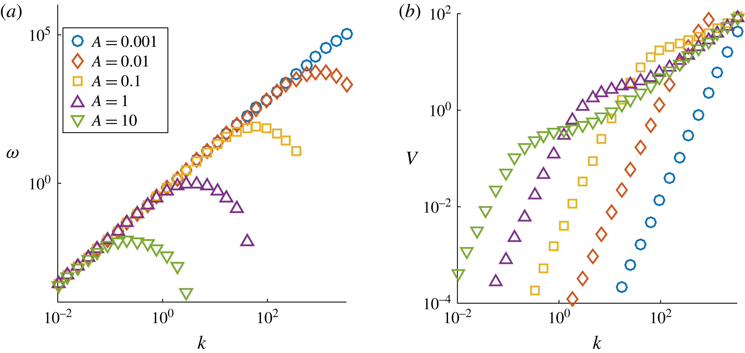
. These are shown in figure 2. The results obtained for the rotational velocity when
 $\unicode[STIX]{x1D6FE}=1/2$
agree well with those obtained by Van Gorder (Reference Van Gorder2015b
) for a helical vortex filament in a Newtonian fluid; this is unsurprising since the motion induced will be dominated by the purely hydrodynamic effects. In Van Gorder (Reference Van Gorder2015b
) the LIA was used to obtain numerical solutions as opposed to the cutoff approximation used here. We see here that the rotational velocity reaches a maximum at particular finite wavenumber
 $k$
; this is in agreement with Van Gorder (Reference Van Gorder2015b
), who found this same result for a helical filament under only hydrodynamic effects. This result shows a good level of agreement between the cutoff approximation used here and the LIA used to regularise the Biot–Savart terms in Van Gorder (Reference Van Gorder2015b
), and hence provides a basis for further comparison between these cases.
Numerical plots of the rotational velocity
 $\unicode[STIX]{x1D714}$
and the translational velocity
 $V$
, of a single helical vortex-current filament using the cutoff approximation to the Biot–Savart integrals. In these plots the modified cutoff parameters
 $\unicode[STIX]{x1D6FC}$
and
 $\unicode[STIX]{x1D6FD}$
are taken to be
 $\unicode[STIX]{x1D6FC}=\unicode[STIX]{x1D6FD}=10^{-5}$
. Different values of the amplitude
 $A$
are shown. Here we have chosen
 $\unicode[STIX]{x1D6FE}=1/2$
. Note that similar results are found for
 $\unicode[STIX]{x1D6FE}=2$
, with only the signs swapped; that is to say,
 $\unicode[STIX]{x1D714}(\unicode[STIX]{x1D6FE}=2)=-\unicode[STIX]{x1D714}(\unicode[STIX]{x1D6FE}=1/2)$
and
 $V(\unicode[STIX]{x1D6FE}=2)=-V(\unicode[STIX]{x1D6FE}=1/2)$
. This makes sense, as when
 $\unicode[STIX]{x1D6FD}=\unicode[STIX]{x1D6FC}$
, the factor
 $1-\unicode[STIX]{x1D6FE}$
will scale the resulting Biot–Savart integral, but will not influence the internal structure of the integral. (a) Rotational velocity
 $\unicode[STIX]{x1D6FE}=1/2$
, (b) translational velocity
 $\unicode[STIX]{x1D6FE}=1/2$
.

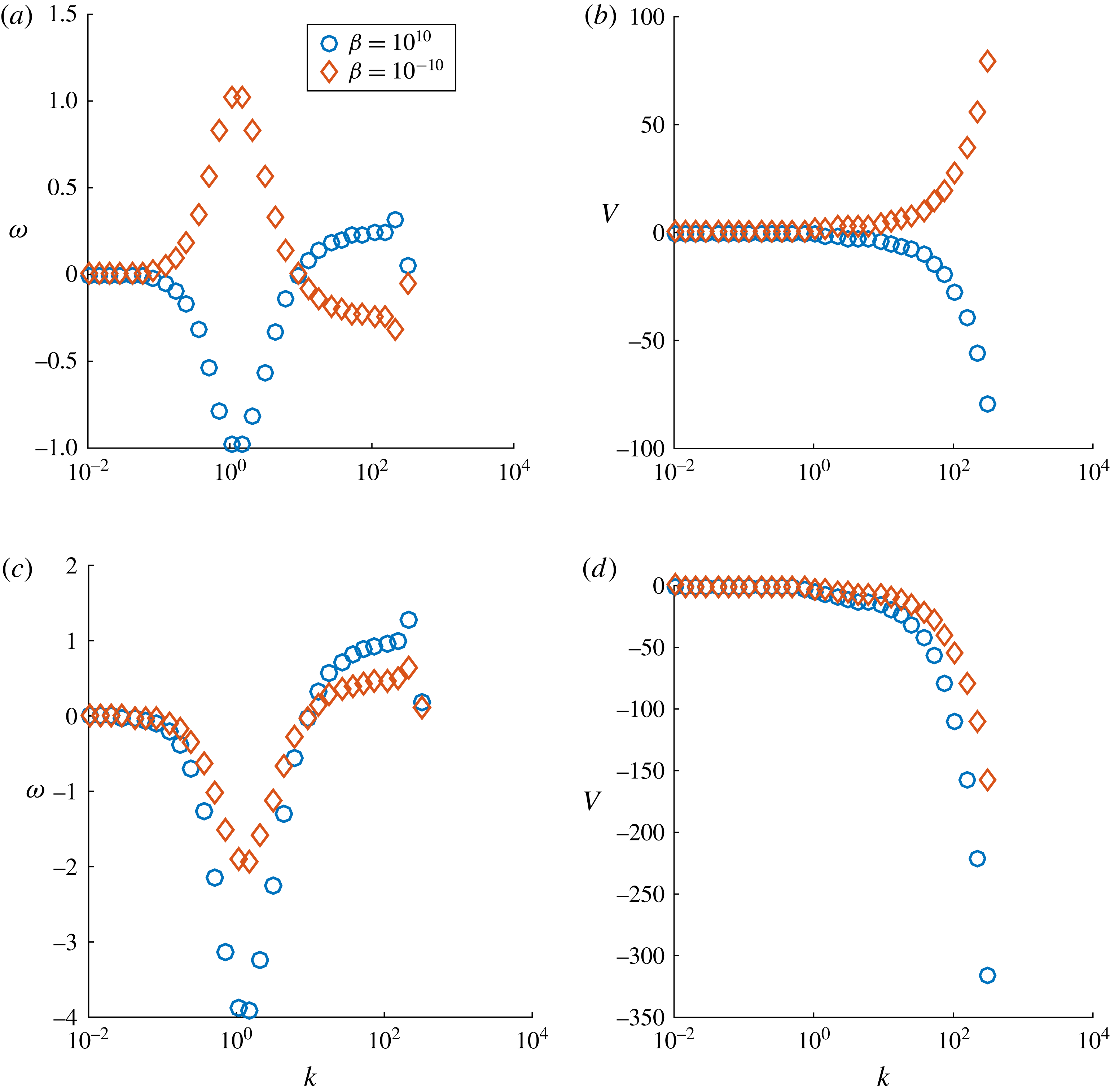
Numerical plots of the rotational velocity
 $\unicode[STIX]{x1D714}$
and the translational velocity
 $V$
of a single helical vortex-current filament using the cutoff approximation to the Biot–Savart integrals. In these plots the modified cutoff parameter
 $\unicode[STIX]{x1D6FC}$
is fixed at
 $10^{-5}$
and the amplitude is fixed at
 $A=1$
. Different values of
 $\unicode[STIX]{x1D6FD}$
are shown in the figure. Here we have again fixed
 $\unicode[STIX]{x1D6FE}=1/2$
in panels (a) and (b) and
 $\unicode[STIX]{x1D6FE}=2$
in panels (c) and (d). As
 $\unicode[STIX]{x1D6FD}$
is a cutoff parameter, introduced to regularise the singularity in the Biot–Savart integral, it is not a physical quantity, but rather a mathematical quantity. That the solutions are not sensitive to it is then useful, as it may be selected for mathematical reasons (to again regularise the solution), without modifying the physics of the current-vortex filaments. (a) Rotational velocity
 $\unicode[STIX]{x1D6FE}=1/2$
, (b) translational velocity
 $\unicode[STIX]{x1D6FE}=1/2$
, (c) rotational velocity
 $\unicode[STIX]{x1D6FE}=2$
, (d) translational velocity
 $\unicode[STIX]{x1D6FE}=2$
.

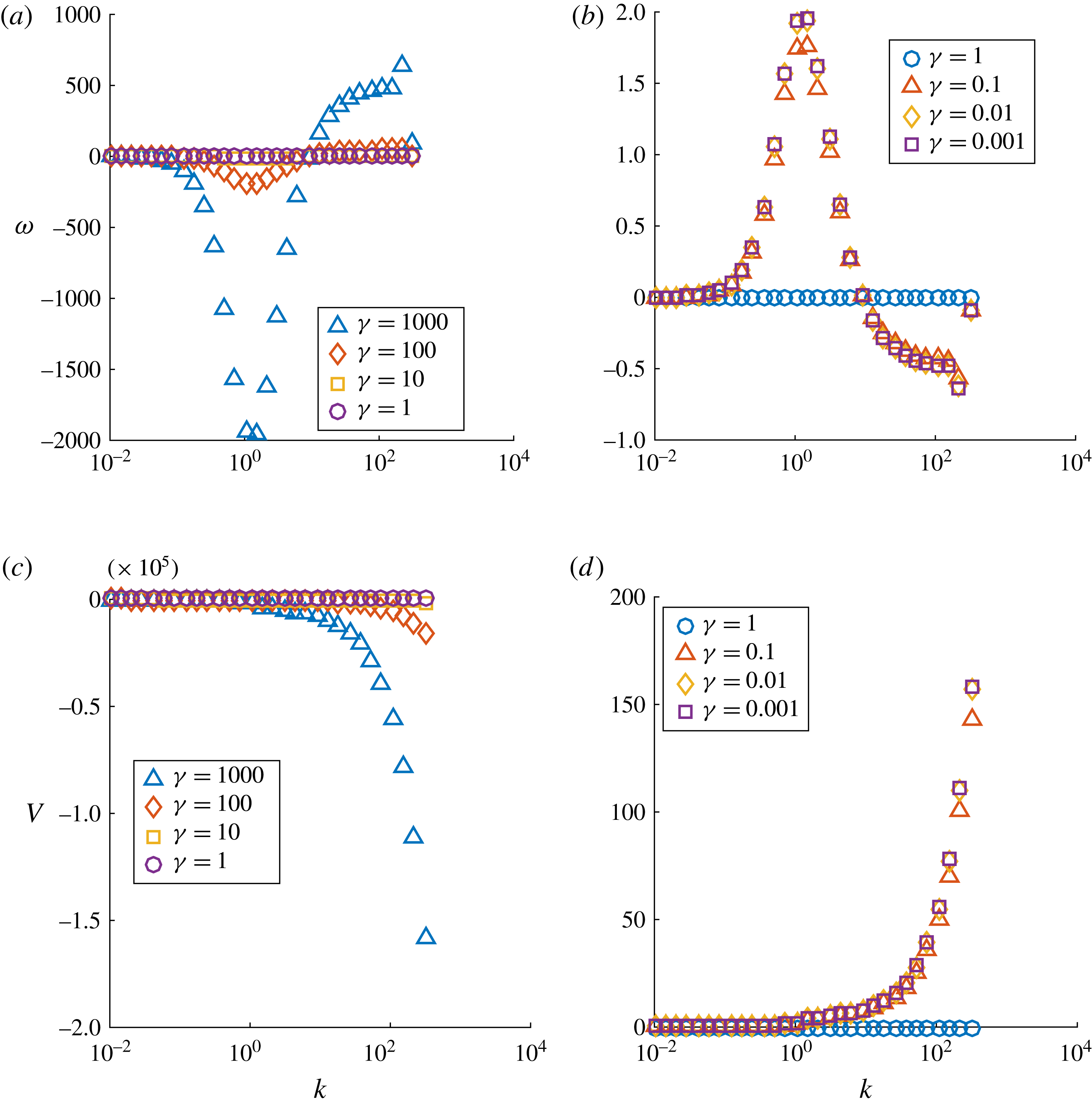
Numerical plots of the rotational velocity
 $\unicode[STIX]{x1D714}$
and the translational velocity
 $V,$
of a single helical vortex-current filament using the cutoff approximation to the Biot–Savart integrals. In these plots the modified cutoff parameters
 $\unicode[STIX]{x1D6FC}$
and
 $\unicode[STIX]{x1D6FD}$
are fixed at
 $10^{-5}$
and the amplitude is fixed at
 $A=1$
. Different values of the parameter
 $\unicode[STIX]{x1D6FE}$
are shown. (a) rotational velocity
 $\unicode[STIX]{x1D6FE}\geqslant 1$
, (b) rotational velocity
 $\unicode[STIX]{x1D6FE}\leqslant 1$
, (c) translational velocity
 $\unicode[STIX]{x1D6FE}\geqslant 1$
, (d) translational velocity
 $\unicode[STIX]{x1D6FE}\leqslant 1$
.

Assuming that the parameters
 $\unicode[STIX]{x1D6FC}$
and
 $\unicode[STIX]{x1D6FD}$
are equal, the parameter
 $\unicode[STIX]{x1D6FE}$
is the only term in this formulation which is influenced by the presence of the MHD effects through the inclusion of the
 $\unicode[STIX]{x1D707}_{0}J^{2}$
term. As such, it is the size of this parameter
 $\unicode[STIX]{x1D6FE}$
which governs the strength of the MHD effects compared to the purely hydrodynamic effects. In figure 2 we assume that
 $\unicode[STIX]{x1D6FC}$
and
 $\unicode[STIX]{x1D6FD}$
are of equal size and that the parameter
 $\unicode[STIX]{x1D6FE}=1/2$
.
The implicit definitions (2.19) and (2.20) imply that the
 $\unicode[STIX]{x1D6FD}$
parameter relates to the strength of the MHD effects whereas
 $\unicode[STIX]{x1D6FC}$
accounts for purely hydrodynamic effects. In figure 3 we have shown the numerical solutions of the system for a range of different
 $\unicode[STIX]{x1D6FD}$
values whilst keeping the fixed value of
 $\unicode[STIX]{x1D6FC}=10^{-5}$
. We can see from the numerical simulations shown in figure 3 that the structure of solutions will not be very sensitive to the values of
 $\unicode[STIX]{x1D6FD}$
used, and it is reasonable to assume that
 $\unicode[STIX]{x1D6FC}=\unicode[STIX]{x1D6FD}$
in the following. Given extreme values of
 $\unicode[STIX]{x1D6FD}$
there can be sign changes in
 $\unicode[STIX]{x1D714}$
and
 $V$
, owing to the fact that very large
 $\unicode[STIX]{x1D6FC}$
or
 $\unicode[STIX]{x1D6FD}$
results in one of the integrals being neglected, but these values are not physically reasonable. Indeed, since both values scale with the radius of vorticity (
 $\unicode[STIX]{x1D6FD}$
) or current (
 $\unicode[STIX]{x1D6FC}$
) within the filament, it makes most physical sense for these parameters to be of the same order, and roughly the same value, as well, for most practical applications.
The only way in which the inclusion of magnetic effects influences the system is through the parameter
 $\unicode[STIX]{x1D6FE}$
. Varying
 $\unicode[STIX]{x1D6FE}$
we find that the hydrodynamic and magnetohydrodynamic effects act to counter one another, that is, the motion induced by the magnetic field will dampen by the motion induced from the purely hydrodynamic effects and this reduces the magnitude of the quantities
 $\unicode[STIX]{x1D714}$
and
 $V$
. Numerical solutions with varying parameter
 $\unicode[STIX]{x1D6FE}$
are shown in figure 4. Note that the values of the wavenumber
 $k$
at which the
 $\unicode[STIX]{x1D714}$
curves change sign and have extreme values (as seen in figure 4) are independent of the value of
 $\unicode[STIX]{x1D6FE}$
. This is because these changes are due to the Biot–Savart integral terms (which depend on
 $A$
,
 $k$
, and on the cutoff parameters), and the factor of
 $1-\unicode[STIX]{x1D6FE}$
will only scale those results.
When
 $\unicode[STIX]{x1D6FE}=1$
, we have that
 $\unicode[STIX]{x1D714}=V=0$
and the motion is completely dampened, that is, the motion induced by the circulation is cancelled by the motion induced by the magnetic field. That there should be some critical value of
 $\unicode[STIX]{x1D6FE}>0$
for which there is a change in the orientation of helical filaments is to be expected, as MHD and hydrodynamic effects should balance one another somewhere in parameter space. That this occurs at
 $\unicode[STIX]{x1D6FE}=1$
is nothing special, as we have just chosen
 $\unicode[STIX]{x1D6FE}$
to represent the ratio of MHD and hydrodynamic effects, and hence
 $\unicode[STIX]{x1D6FE}$
measures their relative strength – as discussed in § 2. Physically this is a measure-zero event, as in real experiments, the accurate selection of MHD and hydrodynamic effects to perfectly cancel is unlikely due to other small perturbations (unaccounted for in the model (2.23)) which would likely push the dynamics into one of the MHD- or hydrodynamic-dominated regimes. Therefore, the value of
 $\unicode[STIX]{x1D6FE}=1$
is best interpreted as a bifurcation between the MHD-dominated regime and the hydrodynamic-dominated regime, rather than having any strong physical significance in its own right.
Some useful observations can be made from these results. Firstly we see that for small values of the parameter,
 $\unicode[STIX]{x1D6FE}\ll 1$
, the behaviour is completely dominated by the hydrodynamic effects and the results compare well with those obtained in Van Gorder (Reference Van Gorder2015b
). As remarked above, when
 $\unicode[STIX]{x1D6FE}=1$
, the contributions cancel and the motion is completely dampened. For large values of
 $\unicode[STIX]{x1D6FE}\gg 1$
, the motion is dominated by the MHD effects, in particular we see that both
 $\unicode[STIX]{x1D714}$
and
 $V$
change sign, i.e. the MHD effects have changed both the direction of rotation,
 $\unicode[STIX]{x1D714}$
and propagation,
 $V$
.
Physically, the results lend support to the idea that helical vortex-current filaments will behave in a similar manner to purely hydrodynamic vortex filaments. The differences are found when MHD and hydrodynamic effects compete, resulting in one of the two dominating. In the case of strong current, the MHD terms result in a reversal of helical filament orientation, resulting in a sign change in the rotational and translational velocities. In terms of structure, however, the helical filament will remain intact. The one exception is if current and vorticity perfectly cancel out, resulting in the helix becoming static (no rotational or translational velocities); however, this is a minor case which is not likely in experiments due to the perfect precision needed.
3.3 Asymptotic scalings of the rotational and translational velocity
To better understand some of these numerical plots of the rotational and translational velocities, we consider asymptotic approximations of the results in (3.9) and (3.10).
We consider the small
 $A$
limit. This is motivated by figure 2. We see that as
 $A$
decreases toward zero, there appears to be a well-defined scaling between both
 $\unicode[STIX]{x1D714}$
and
 $V$
with
 $k$
. We shall also assume
 $\unicode[STIX]{x1D6FD}=\unicode[STIX]{x1D6FC}$
. In the small
 $A$
limit, (3.9) reduces to
 $$\begin{eqnarray}\displaystyle \unicode[STIX]{x1D714}=(\unicode[STIX]{x1D6FE}-1)\int _{\unicode[STIX]{x1D6FC}}^{\infty }\frac{1-k\unicode[STIX]{x1D70E}\sin (k\unicode[STIX]{x1D70E})-\cos (k\unicode[STIX]{x1D70E})}{\unicode[STIX]{x1D70E}^{3}}\,\text{d}\unicode[STIX]{x1D70E}+O(\unicode[STIX]{x1D6FC}^{2})+O(A^{2}). & & \displaystyle\end{eqnarray}$$
Evaluating the integral, and noting that only the contribution at
 $\unicode[STIX]{x1D6FC}$
matters (the far-field contribution decays like
 $\unicode[STIX]{x1D70E}^{-2}$
as
 $\unicode[STIX]{x1D70E}\rightarrow \infty$
), we have
 $$\begin{eqnarray}\displaystyle \unicode[STIX]{x1D714}=(\unicode[STIX]{x1D6FE}-1)\left(\frac{1}{2}\ln (k)+\frac{1}{2}\ln (\unicode[STIX]{x1D6FC})+\frac{2\unicode[STIX]{x1D6E4}_{\text{EM}}-1}{4}\right)k^{2}++O(\unicode[STIX]{x1D6FC}^{2})+O(A^{2}), & & \displaystyle\end{eqnarray}$$
where
 $\unicode[STIX]{x1D6E4}_{EM}$
is the Euler–Mascheroni constant (
 $\unicode[STIX]{x1D6E4}_{\text{EM}}\approx 0.5772$
). Therefore, for small enough
 $A$
,
 $\unicode[STIX]{x1D714}$
scales as a quadratic with the wavenumber
 $k$
. The sign of the quadratic will depend on the size of
 $\unicode[STIX]{x1D6FE}$
. For
 $\unicode[STIX]{x1D6FE}<1$
we have that the relation will be
 $\unicode[STIX]{x1D714}\sim k^{2}$
, while when
 $\unicode[STIX]{x1D6FE}>0$
we have that
 $\unicode[STIX]{x1D714}\sim -k^{2}$
. These asymptotic scalings are in complete agreement with what we show in figure 2.
One can perform similar computations in order to obtain an asymptotic expansion for the translational velocity,
 $V$
, in the small
 $A$
regime. We obtain
 $$\begin{eqnarray}\displaystyle V=(\unicode[STIX]{x1D6FE}-1)\left(\frac{1}{2}\ln (k)+\frac{1}{2}\ln (\unicode[STIX]{x1D6FC})+\frac{2\unicode[STIX]{x1D6E4}_{\text{EM}}-3}{4}\right)k^{3}A^{2}++O(\unicode[STIX]{x1D6FC}^{2})+O(A^{4}), & & \displaystyle\end{eqnarray}$$
hence the scaling is
 $V\sim A^{2}k^{3}$
for the hydrodynamic regime of
 $\unicode[STIX]{x1D6FE}<1$
, and
 $V\sim -A^{2}k^{3}$
for the MHD regime of
 $\unicode[STIX]{x1D6FE}>1$
. Again, these scalings are in agreement with what is seen in figure 2.
For larger
 $A$
, the dynamics is more fundamentally nonlinear, and hence the behaviour of
 $\unicode[STIX]{x1D714}$
becomes non-monotone in the wavenumber
 $k$
. Thus, one must investigate the resulting integrals numerically in these regimes.
4 Planar vortex-current filaments
One important and rather fundamental solution to the LIA is the planar vortex filament, which was first found by Da Rios (Da Rios Reference Da Rios1906; Ricca Reference Ricca1996) and also studied later by Hasimoto (Reference Hasimoto1971) in curvature-torsion coordinates, and related the solution to elastica. The solution takes the form of a plane curve, with the motion being rotational orthogonal to the plane in which the curve lies. Kida (Reference Kida1981) compared the planar filament with other types of solutions. A direct derivation in Cartesian coordinates was given in Van Gorder (Reference Van Gorder2012b ). The Poincaré–Lindstedt method was used to study the spatial structure of a spatially periodic planar filament in the Cartesian frame by Van Gorder (Reference Van Gorder2013b ). In this approach, deviations from a centrally aligned reference axis were taken to be the small parameter, and an approximate closed form of the solutions was given without the need for the inversion of elliptic integrals (which would be required for an exact representation). Kida (Reference Kida1982) considered a stability analysis for the planar filament (with the analysis performed numerically), while Van Gorder (Reference Van Gorder2013a ) was able to obtain an analytical stability result for the orbital stability (spectral stability). Fukumoto (Reference Fukumoto1997) studied the influence of background flows on planar filaments. In addition to the standard curvature-torsion frame (used by Hasimoto (Reference Hasimoto1971)) or the Cartesian frame (used by Van Gorder (Reference Van Gorder2013b )), there is an alternate formulation, given by Umeki (Reference Umeki2010), which formulates the LIA in terms of the unknown tangent vector as a function of arclength and time. A planar solution in this framework was given by Van Gorder (Reference Van Gorder2012a ). The planar vortex filament solution was also recently shown to exist for the non-local Biot–Savart dynamics (Van Gorder Reference Van Gorder2015c ).
It is a natural to ask whether such solutions exist in the presence of MHD effects, which is what we shall investigate here. A general planar filament can be written in the form
 $$\begin{eqnarray}\displaystyle \boldsymbol{r}(x,t)=(x,\cos (\unicode[STIX]{x1D6FA}t)\unicode[STIX]{x1D713}(x),\sin (\unicode[STIX]{x1D6FA}t)\unicode[STIX]{x1D713}(x)), & & \displaystyle\end{eqnarray}$$
where
 $\unicode[STIX]{x1D713}$
is a real-valued, twice differentiable function of position alone. As before, the constant
 $\unicode[STIX]{x1D714}$
has the interpretation of being the rotational velocity of the filament. This representation used here describes a rotating filament which is aligned along a plane intersecting the
 $x$
-axis.
Determining the planar filament in the MHD formulation above is more challenging than for the helical filament which we have focused on thus far. We showed that the helical filament,
 $\boldsymbol{r}(x,t)=(x+Vt,A\cos (kx-\unicode[STIX]{x1D714}t+x_{0}),A\sin (kx-\unicode[STIX]{x1D714}t+x_{0}))$
, can be solved for exactly in that the motion parameters
 $\unicode[STIX]{x1D714}$
and
 $V$
can be determined in terms of the other model parameters.
Assuming a solution of the form (4.1), the time evolution of the filament as governed by the MHD vortex model, equation (2.18) is given by
 $$\begin{eqnarray}\displaystyle \boldsymbol{r}_{t}(x,t) & = & \displaystyle -\frac{\unicode[STIX]{x1D6FE}}{2}\int _{\mathbb{R}}\frac{[\boldsymbol{r}(x,t)-\boldsymbol{r}(s,t)]\times (\text{d}s,\cos (\unicode[STIX]{x1D6FA}t)\unicode[STIX]{x1D713}^{\prime }(s)\,\text{d}s,\sin (\unicode[STIX]{x1D6FA}t)\unicode[STIX]{x1D713}^{\prime }(s)\,\text{d}s)}{[|\boldsymbol{r}(x,t)-\boldsymbol{r}(s,t)|^{2}+\unicode[STIX]{x1D6FC}^{2}]^{3/2}}\nonumber\\ \displaystyle & & \displaystyle +\,\frac{1}{2}\int _{\mathbb{R}}\frac{[\boldsymbol{r}(x,t)-\boldsymbol{r}(s,t)]\times (\text{d}s,\cos (\unicode[STIX]{x1D6FA}t)\unicode[STIX]{x1D713}^{\prime }(s)\,\text{d}s,\sin (\unicode[STIX]{x1D6FA}t)\unicode[STIX]{x1D713}^{\prime }(s)\,\text{d}s)}{[|\boldsymbol{r}(x,t)-\boldsymbol{r}(s,t)|^{2}+\unicode[STIX]{x1D6FD}^{2}]^{3/2}}.\end{eqnarray}$$
Here
 $\boldsymbol{r}_{t}$
is the time derivative of the planar filament and
 $\text{d}\boldsymbol{r}(s,t)=(1,\cos (\unicode[STIX]{x1D6FA}t)\unicode[STIX]{x1D713}^{\prime }(s),\sin (\unicode[STIX]{x1D6FA}t)\unicode[STIX]{x1D713}^{\prime }(s))\,\text{d}s=(\text{d}s,\cos (\unicode[STIX]{x1D6FA}t)\unicode[STIX]{x1D713}^{\prime }(s)\,\text{d}s,\sin (\unicode[STIX]{x1D6FA}t)\unicode[STIX]{x1D713}^{\prime }(s)\,\text{d}s)$
for the planar filament given in the form (4.1).
We then calculate
 $$\begin{eqnarray}\displaystyle |\boldsymbol{r}(s,t)-\boldsymbol{r}(x,t)| & = & \displaystyle (s-x)^{2}+\cos ^{2}(\unicode[STIX]{x1D6FA}t)(\unicode[STIX]{x1D713}(s)-\unicode[STIX]{x1D713}(x))^{2}+\sin ^{2}(\unicode[STIX]{x1D6FA}t)(\unicode[STIX]{x1D713}(s)-\unicode[STIX]{x1D713}(x))^{2}\nonumber\\ \displaystyle & = & \displaystyle (s-x)^{2}+(\unicode[STIX]{x1D713}(s)-\unicode[STIX]{x1D713}(x))^{2},\end{eqnarray}$$
 $$\begin{eqnarray}\displaystyle & & \displaystyle (\boldsymbol{r}(s,t)-\boldsymbol{r}(x,t))\times (\text{d}s,\cos (\unicode[STIX]{x1D6FA}t)\unicode[STIX]{x1D713}^{\prime }(s)\,\text{d}s,\sin (\unicode[STIX]{x1D6FA}t)\unicode[STIX]{x1D713}^{\prime }(s)\,\text{d}s)\nonumber\\ \displaystyle & & \displaystyle \quad =\left(0,\sin (\unicode[STIX]{x1D6FA}t)[(\unicode[STIX]{x1D713}(x)-\unicode[STIX]{x1D713}(s))-(x-s)\unicode[STIX]{x1D713}^{\prime }(s)]\,\text{d}s,\right.\nonumber\\ \displaystyle & & \displaystyle \left.\qquad -\cos (\unicode[STIX]{x1D6FA}t)[(\unicode[STIX]{x1D713}(x)-\unicode[STIX]{x1D713}(s))-(x-s)\unicode[STIX]{x1D713}^{\prime }(s)]\,\text{d}s\right),\end{eqnarray}$$
and
 $$\begin{eqnarray}\displaystyle \boldsymbol{r}_{t}(x,t)=(0,-\unicode[STIX]{x1D6FA}\sin (\unicode[STIX]{x1D6FA}t)\unicode[STIX]{x1D713}(x),\unicode[STIX]{x1D6FA}\cos (\unicode[STIX]{x1D6FA}t)\unicode[STIX]{x1D713}(x)), & & \displaystyle\end{eqnarray}$$
and substitution of these into (4.2) gives the system of equations
 $$\begin{eqnarray}\displaystyle X:\quad 0=0, & & \displaystyle\end{eqnarray}$$
 $$\begin{eqnarray}\displaystyle Y:\quad -\unicode[STIX]{x1D6FA}\sin (\unicode[STIX]{x1D6FA}t)\unicode[STIX]{x1D713}(x) & = & \displaystyle -\sin (\unicode[STIX]{x1D6FA}t)\frac{\unicode[STIX]{x1D6FE}}{2}\int _{\mathbb{R}}\frac{(\unicode[STIX]{x1D713}(s)-\unicode[STIX]{x1D713}(x))-(s-x)\unicode[STIX]{x1D713}^{\prime }(s)}{[(s-x)^{2}+(\unicode[STIX]{x1D713}(s)-\unicode[STIX]{x1D713}(x))^{2}+\unicode[STIX]{x1D6FC}^{2}]^{3/2}}\text{d}s\nonumber\\ \displaystyle & & \displaystyle +\,\sin (\unicode[STIX]{x1D6FA}t)\frac{1}{2}\int _{\mathbb{R}}\frac{(\unicode[STIX]{x1D713}(s)-\unicode[STIX]{x1D713}(x))-(s-x)\unicode[STIX]{x1D713}^{\prime }(s)}{[(s-x)^{2}+(\unicode[STIX]{x1D713}(s)-\unicode[STIX]{x1D713}(x))^{2}+\unicode[STIX]{x1D6FD}^{2}]^{3/2}}\text{d}s,\end{eqnarray}$$
 $$\begin{eqnarray}\displaystyle Z:\quad -\unicode[STIX]{x1D6FA}\cos (\unicode[STIX]{x1D6FA}t)\unicode[STIX]{x1D713}(x) & = & \displaystyle -\cos (\unicode[STIX]{x1D6FA}t)\frac{\unicode[STIX]{x1D6FE}}{2}\int _{\mathbb{R}}\frac{(\unicode[STIX]{x1D713}(s)-\unicode[STIX]{x1D713}(x))-(s-x)\unicode[STIX]{x1D713}^{\prime }(s)}{[(s-x)^{2}+(\unicode[STIX]{x1D713}(s)-\unicode[STIX]{x1D713}(x))^{2}+\unicode[STIX]{x1D6FC}^{2}]^{3/2}}\text{d}s\nonumber\\ \displaystyle & & \displaystyle +\,\cos (\unicode[STIX]{x1D6FA}t)\frac{1}{2}\int _{\mathbb{R}}\frac{(\unicode[STIX]{x1D713}(s)-\unicode[STIX]{x1D713}(x))-(s-x)\unicode[STIX]{x1D713}^{\prime }(s)}{[(s-x)^{2}+(\unicode[STIX]{x1D713}(s)-\unicode[STIX]{x1D713}(x))^{2}+\unicode[STIX]{x1D6FD}^{2}]^{3/2}}\text{d}s,\end{eqnarray}$$
for the
 $X$
,
 $Y$
and
 $Z$
components respectively. The two non-trivial equations are equivalent, hence we may write equations (4.7) and (4.8) as an equivalent singular integral equation
 $$\begin{eqnarray}\displaystyle & & \displaystyle \unicode[STIX]{x1D6FA}\unicode[STIX]{x1D713}(x)+\frac{\unicode[STIX]{x1D6FE}}{2}\int _{\mathbb{R}}\frac{(s-x)\unicode[STIX]{x1D713}^{\prime }(s)-(\unicode[STIX]{x1D713}(s)-\unicode[STIX]{x1D713}(x))}{[(s-x)^{2}+(\unicode[STIX]{x1D713}(s)-\unicode[STIX]{x1D713}(x))^{2}+\unicode[STIX]{x1D6FC}^{2}]^{3/2}}\,\text{d}s\nonumber\\ \displaystyle & & \displaystyle \quad -\,\frac{1}{2}\int _{\mathbb{R}}\frac{(s-x)\unicode[STIX]{x1D713}^{\prime }(s)-(\unicode[STIX]{x1D713}(s)-\unicode[STIX]{x1D713}(x))}{[(s-x)^{2}+(\unicode[STIX]{x1D713}(s)-\unicode[STIX]{x1D713}(x))^{2}+\unicode[STIX]{x1D6FD}^{2}]^{3/2}}\,\text{d}s=0.\end{eqnarray}$$
We shall apply the analytical approach of Van Gorder (Reference Van Gorder2015c
) to the solution of (4.9). In the limit where
 $\unicode[STIX]{x1D6FC}$
and
 $\unicode[STIX]{x1D6FD}$
are negligibly small, so that we take the cutoff effects to zero, equation (4.9) reduces to the nonlinear integral equation
 $$\begin{eqnarray}\displaystyle \unicode[STIX]{x1D713}(x)+\unicode[STIX]{x1D706}\int _{\mathbb{R}}\frac{(\unicode[STIX]{x1D713}(x)-\unicode[STIX]{x1D713}(s))-(x-s)\unicode[STIX]{x1D713}^{\prime }(s)}{[(s-x)^{2}+(\unicode[STIX]{x1D713}(s)-\unicode[STIX]{x1D713}(x))^{2}]^{3/2}}\,\text{d}s=0, & & \displaystyle\end{eqnarray}$$
with eigenvalue
 $$\begin{eqnarray}\displaystyle \unicode[STIX]{x1D706}=-\frac{1-\unicode[STIX]{x1D6FE}}{2\unicode[STIX]{x1D6FA}}. & & \displaystyle\end{eqnarray}$$
In the very special case where hydrodynamic and MHD effects balance,
 $\unicode[STIX]{x1D6FE}=1$
and we have
 $\unicode[STIX]{x1D706}=0$
, so
 $\unicode[STIX]{x1D713}(x)=0$
. This gives a line filament. Therefore, we shall consider the case of
 $\unicode[STIX]{x1D6FE}\neq 1$
throughout the remainder of this section.
We then regularise using the LIA in the core region, as was done in Van Gorder (Reference Van Gorder2015c ), from which we obtain the nonlinear integro-differential equation
 $$\begin{eqnarray}\displaystyle \unicode[STIX]{x1D713}+\unicode[STIX]{x1D706}\ln (\unicode[STIX]{x1D6FF}^{-1})\unicode[STIX]{x1D713}^{\prime \prime }+\unicode[STIX]{x1D706}\int _{|s-x|>\unicode[STIX]{x1D6FF}}\frac{(\unicode[STIX]{x1D713}(x)-\unicode[STIX]{x1D713}(s))-(x-s)\unicode[STIX]{x1D713}^{\prime }(s)}{[(s-x)^{2}+(\unicode[STIX]{x1D713}(s)-\unicode[STIX]{x1D713}(x))^{2}]^{3/2}}\,\text{d}s=0, & & \displaystyle\end{eqnarray}$$
where
 $\unicode[STIX]{x1D6FF}\ll 1$
is the small parameter used in the regularisation. In this approach, we rely on the LIA accurately approximating the core region for
 $s\approx x$
, while we keep the Biot–Savart integral term in regions where the LIA loses accuracy.
As in Van Gorder (Reference Van Gorder2015c ), we may apply a strained-parameter approach in order to obtain an analytical approximation to the solution of (4.12). Assume that the amplitude of the deviations from the reference axis are sufficiently small (which is a physically reasonable assumption) and then expand the solution in the amplitude parameter like
 $$\begin{eqnarray}\displaystyle \unicode[STIX]{x1D713}(x)=A\unicode[STIX]{x1D6F9}_{0}(\unicode[STIX]{x1D712})+A^{3}\unicode[STIX]{x1D6F9}_{1}(\unicode[STIX]{x1D712})+O(A^{5}), & & \displaystyle\end{eqnarray}$$
for
 $|A|<1$
, where
 $\unicode[STIX]{x1D712}=\unicode[STIX]{x1D709}_{0}(1+\unicode[STIX]{x1D709}_{1}A^{2}+O(A^{4}))x$
is the strained space variable.
Without loss of generality, we take
 $\unicode[STIX]{x1D6F9}_{0}(0)=1$
,
 $\unicode[STIX]{x1D6F9}_{0}^{\prime }(0)=0$
so that the maximal amplitude of
 $\unicode[STIX]{x1D713}$
occurs at
 $x=0$
. We also take
 $\unicode[STIX]{x1D6F9}_{1}(0)=\unicode[STIX]{x1D6F9}_{1}^{\prime }(0)=0$
. The parameter
 $\unicode[STIX]{x1D709}_{1}$
will be selected in order to remove secular terms. We place (4.13) into integro-differential equation (4.12), expand in the small parameter
 $A$
, and then match powers of
 $A$
. From the form of (4.12), we obtain terms with second derivatives as well as terms from the integral. We find that
 $$\begin{eqnarray}\displaystyle \unicode[STIX]{x1D709}_{0}^{2}\unicode[STIX]{x1D706}\ln (\unicode[STIX]{x1D6FF}^{-1})\frac{\text{d}^{2}\unicode[STIX]{x1D6F9}_{0}}{\text{d}\unicode[STIX]{x1D712}^{2}}+\unicode[STIX]{x1D6F9}_{0}+\unicode[STIX]{x1D706}I_{0}[\unicode[STIX]{x1D6F9}_{0}]=0, & & \displaystyle\end{eqnarray}$$
 $$\begin{eqnarray}\unicode[STIX]{x1D709}_{0}^{2}\unicode[STIX]{x1D706}\ln (\unicode[STIX]{x1D6FF}^{-1})\frac{\text{d}^{2}\unicode[STIX]{x1D6F9}_{1}}{\text{d}\unicode[STIX]{x1D712}^{2}}+\unicode[STIX]{x1D6F9}_{1}+\unicode[STIX]{x1D706}I_{0}[\unicode[STIX]{x1D6F9}_{1}]=\unicode[STIX]{x1D709}_{0}^{2}\unicode[STIX]{x1D706}\ln (\unicode[STIX]{x1D6FF}^{-1})\left\{\frac{3}{2}\unicode[STIX]{x1D709}_{0}^{2}\left(\frac{\text{d}\unicode[STIX]{x1D6F9}_{0}}{\text{d}\unicode[STIX]{x1D712}}\right)^{2}-2\unicode[STIX]{x1D709}_{1}\right\}\frac{\text{d}^{2}\unicode[STIX]{x1D6F9}_{0}}{\text{d}\unicode[STIX]{x1D712}^{2}}-\unicode[STIX]{x1D706}I_{1}[\unicode[STIX]{x1D6F9}_{0}],\end{eqnarray}$$
where the integral operators
 $I_{0}$
and
 $I_{1}$
are given by
 $$\begin{eqnarray}\displaystyle I_{0}[u(\unicode[STIX]{x1D712})]=\int _{\unicode[STIX]{x1D6FF}}^{\infty }\frac{u^{\prime }(\unicode[STIX]{x1D712}+\unicode[STIX]{x1D70E})-u^{\prime }(\unicode[STIX]{x1D712}-\unicode[STIX]{x1D70E})}{\unicode[STIX]{x1D70E}^{2}}\,\text{d}\unicode[STIX]{x1D70E}-\int _{\unicode[STIX]{x1D6FF}}^{\infty }\frac{u(\unicode[STIX]{x1D712}+\unicode[STIX]{x1D70E})+u(\unicode[STIX]{x1D712}-\unicode[STIX]{x1D70E})-2u(\unicode[STIX]{x1D712})}{\unicode[STIX]{x1D70E}^{3}}\,\text{d}\unicode[STIX]{x1D70E}, & & \displaystyle \nonumber\\ \displaystyle & & \displaystyle\end{eqnarray}$$
 $$\begin{eqnarray}\displaystyle I_{1}[u(\unicode[STIX]{x1D712})] & = & \displaystyle \frac{3}{2}\int _{\unicode[STIX]{x1D6FF}}^{\infty }\frac{\{u(\unicode[STIX]{x1D712}-\unicode[STIX]{x1D70E})-u(\unicode[STIX]{x1D712})\}u^{\prime }(\unicode[STIX]{x1D712}-\unicode[STIX]{x1D70E})}{\unicode[STIX]{x1D70E}^{4}}\,\text{d}\unicode[STIX]{x1D70E}\nonumber\\ \displaystyle & & \displaystyle -\,\frac{3}{2}\int _{\unicode[STIX]{x1D6FF}}^{\infty }\frac{\{u(\unicode[STIX]{x1D712}+\unicode[STIX]{x1D70E})-u(\unicode[STIX]{x1D712})\}u^{\prime }(\unicode[STIX]{x1D712}+\unicode[STIX]{x1D70E})}{\unicode[STIX]{x1D70E}^{4}}\,\text{d}\unicode[STIX]{x1D70E}\nonumber\\ \displaystyle & & \displaystyle +\,\frac{3}{2}\int _{\unicode[STIX]{x1D6FF}}^{\infty }\frac{\{u(\unicode[STIX]{x1D712}-\unicode[STIX]{x1D70E})-u(\unicode[STIX]{x1D712})\}^{2}}{\unicode[STIX]{x1D70E}^{5}}\,\text{d}\unicode[STIX]{x1D70E}+\frac{3}{2}\int _{\unicode[STIX]{x1D6FF}}^{\infty }\frac{\{u(\unicode[STIX]{x1D712}+\unicode[STIX]{x1D70E})-u(\unicode[STIX]{x1D712})\}^{2}}{\unicode[STIX]{x1D70E}^{5}}\,\text{d}\unicode[STIX]{x1D70E}.\end{eqnarray}$$
We shall pick
 $\unicode[STIX]{x1D709}_{0}$
from (4.14) and then
 $\unicode[STIX]{x1D702}$
to remove secular terms from (4.15). We find
 $$\begin{eqnarray}\displaystyle \unicode[STIX]{x1D709}_{0}=\sqrt{\frac{1-\unicode[STIX]{x1D706}\displaystyle \frac{1+\unicode[STIX]{x1D6FF}^{2}\text{Ci}(\unicode[STIX]{x1D6FF})-\unicode[STIX]{x1D6FF}\sin (\unicode[STIX]{x1D6FF})-\cos (\unicode[STIX]{x1D6FF})}{\unicode[STIX]{x1D6FF}^{2}}}{\unicode[STIX]{x1D706}\ln (\unicode[STIX]{x1D6FF}^{-1})}}, & & \displaystyle\end{eqnarray}$$
where we have the asymptotic scaling
 $$\begin{eqnarray}\displaystyle 1-\unicode[STIX]{x1D706}\frac{1+\unicode[STIX]{x1D6FF}^{2}\text{Ci}(\unicode[STIX]{x1D6FF})-\unicode[STIX]{x1D6FF}\sin (\unicode[STIX]{x1D6FF})-\cos (\unicode[STIX]{x1D6FF})}{\unicode[STIX]{x1D6FF}^{2}}=1-\unicode[STIX]{x1D706}\left(\ln (\unicode[STIX]{x1D6FF})+\unicode[STIX]{x1D6E4}_{\text{EM}}-\frac{1}{2}-\frac{1}{8}\unicode[STIX]{x1D6FF}^{2}+O(\unicode[STIX]{x1D6FF}^{4})\right) & & \displaystyle\end{eqnarray}$$
for small
 $\unicode[STIX]{x1D6FF}>0$
. Again,
 $\unicode[STIX]{x1D6E4}_{\text{EM}}$
is the Euler–Mascheroni constant.
A bounded periodic solution will only exist for real
 $\unicode[STIX]{x1D709}_{0}$
, so we ensure that the factor within the square root in (4.18) is positive. Manipulation of this quantity gives the condition
 $$\begin{eqnarray}\displaystyle -\frac{2\unicode[STIX]{x1D6FA}}{1-\unicode[STIX]{x1D6FE}}=\frac{1}{\unicode[STIX]{x1D706}}>\left(\ln (\unicode[STIX]{x1D6FF})+\unicode[STIX]{x1D6E4}_{\text{EM}}-\frac{1}{2}-\frac{1}{8}\unicode[STIX]{x1D6FF}^{2}+O(\unicode[STIX]{x1D6FF}^{4})\right). & & \displaystyle\end{eqnarray}$$
When
 $\unicode[STIX]{x1D6FA}$
and
 $\unicode[STIX]{x1D6FE}$
permit this inequality to hold, then we have that bounded periodic solutions are possible. This gives the order-zero term
 $\unicode[STIX]{x1D6F9}_{0}(\unicode[STIX]{x1D712})=\cos (\unicode[STIX]{x1D712})$
.
Next, to remove the secular terms from (4.15) which result from the choice of
 $\unicode[STIX]{x1D6F9}_{0}(\unicode[STIX]{x1D712})$
, we must pick
 $$\begin{eqnarray}\displaystyle \unicode[STIX]{x1D709}_{1}={\textstyle \frac{3}{16}}\unicode[STIX]{x1D709}_{0}^{2}. & & \displaystyle\end{eqnarray}$$
With secular terms removed, the solution to (4.15) takes the form
 $$\begin{eqnarray}\displaystyle \unicode[STIX]{x1D6F9}_{1}(\unicode[STIX]{x1D712})=\unicode[STIX]{x1D6F9}_{11}(\cos (\unicode[STIX]{x1D712})-\cos (2\unicode[STIX]{x1D712}))+\unicode[STIX]{x1D6F9}_{12}(\cos (\unicode[STIX]{x1D712})-\cos (3\unicode[STIX]{x1D712})), & & \displaystyle\end{eqnarray}$$
and we find that the constants
 $\unicode[STIX]{x1D6F9}_{11}$
and
 $\unicode[STIX]{x1D6F9}_{12}$
are given by
 $$\begin{eqnarray}\displaystyle \unicode[STIX]{x1D6F9}_{11} & = & \displaystyle \frac{\unicode[STIX]{x1D706}\{\unicode[STIX]{x1D6FF}^{4}[\text{Ci}(\unicode[STIX]{x1D6FF})-8\text{Ci}(2\unicode[STIX]{x1D6FF})]+(6+\unicode[STIX]{x1D6FF}^{2})\cos (\unicode[STIX]{x1D6FF})-(3+2\unicode[STIX]{x1D6FF}^{2})\cos (2\unicode[STIX]{x1D6FF})\}}{8\unicode[STIX]{x1D716}^{2}\{3\unicode[STIX]{x1D6FF}^{2}+\unicode[STIX]{x1D706}(4\unicode[STIX]{x1D6FF}^{2}[\text{Ci}(\unicode[STIX]{x1D6FF})-\text{Ci}(2\unicode[STIX]{x1D6FF})]+2\unicode[STIX]{x1D6FF}[\sin (2\unicode[STIX]{x1D6FF})-2\sin (\unicode[STIX]{x1D6FF})]+\cos (2\unicode[STIX]{x1D6FF})-4\cos (\unicode[STIX]{x1D6FF})+3)\}}\nonumber\\ \displaystyle & & \displaystyle +\,\frac{\unicode[STIX]{x1D706}\{\unicode[STIX]{x1D6FF}^{4} [(2\unicode[STIX]{x1D6FF}-\unicode[STIX]{x1D6FF}^{3})\sin (\unicode[STIX]{x1D6FF})+(4\unicode[STIX]{x1D6FF}^{3}-2\unicode[STIX]{x1D6FF})\sin (2\unicode[STIX]{x1D6FF})-3\}}{8\unicode[STIX]{x1D716}^{2}\{3\unicode[STIX]{x1D6FF}^{2}+\unicode[STIX]{x1D706}(4\unicode[STIX]{x1D6FF}^{2}[\text{Ci}(\unicode[STIX]{x1D6FF})-\text{Ci}(2\unicode[STIX]{x1D6FF})]+2\unicode[STIX]{x1D6FF}[\sin (2\unicode[STIX]{x1D6FF})-2\sin (\unicode[STIX]{x1D6FF})]+\cos (2\unicode[STIX]{x1D6FF})-4\cos (\unicode[STIX]{x1D6FF})+3)\}},\nonumber\\ \displaystyle & & \displaystyle\end{eqnarray}$$
 $$\begin{eqnarray}\displaystyle & & \displaystyle \unicode[STIX]{x1D6F9}_{12}=\frac{3}{8\unicode[STIX]{x1D706}\unicode[STIX]{x1D6FF}^{2}\ln (\unicode[STIX]{x1D6FF}^{-1})}\nonumber\\ \displaystyle & & \displaystyle \quad \times \,\frac{(\unicode[STIX]{x1D6FF}^{2}+\unicode[STIX]{x1D706}+\unicode[STIX]{x1D6FF}^{2}\text{Ci}(\unicode[STIX]{x1D6FF})\unicode[STIX]{x1D706}-\unicode[STIX]{x1D6FF}\sin (\unicode[STIX]{x1D6FF})\unicode[STIX]{x1D706}-\cos (\unicode[STIX]{x1D6FF})\unicode[STIX]{x1D706})^{2}}{8\unicode[STIX]{x1D6FF}^{2}+\unicode[STIX]{x1D706}(8+9\unicode[STIX]{x1D6FF}^{2}[\text{Ci}(\unicode[STIX]{x1D6FF})-\text{Ci}(3\unicode[STIX]{x1D6FF})]+3\unicode[STIX]{x1D6FF}[\sin (3\unicode[STIX]{x1D6FF})-3\sin (\unicode[STIX]{x1D6FF})]+\cos (3\unicode[STIX]{x1D6FF})-9\cos (\unicode[STIX]{x1D6FF}))}.\nonumber\\ \displaystyle & & \displaystyle\end{eqnarray}$$
Here
 $\text{Ci}$
denotes the cosine integral
 $$\begin{eqnarray}\displaystyle \text{Ci}(x)=-\int _{x}^{\infty }\frac{\cos (q)}{q}\,\text{d}q=\unicode[STIX]{x1D6E4}_{\text{EM}}+\ln (x)+\int _{0}^{x}\frac{\cos (q)-1}{q}\,\text{d}q. & & \displaystyle\end{eqnarray}$$
For small
 $\unicode[STIX]{x1D6FF}>0$
, these coefficients behave like
 $$\begin{eqnarray}\displaystyle & \displaystyle \unicode[STIX]{x1D6F9}_{11}=\unicode[STIX]{x1D706}\frac{84\unicode[STIX]{x1D6E4}_{\text{EM}}+84\ln (\unicode[STIX]{x1D6FF})+96\ln (2)-133}{384\ln (2)\unicode[STIX]{x1D706}-288}+O(\unicode[STIX]{x1D6FF}^{2}), & \displaystyle\end{eqnarray}$$
 $$\begin{eqnarray}\displaystyle & \displaystyle \unicode[STIX]{x1D6F9}_{12}=\frac{3}{32\unicode[STIX]{x1D706}\ln (\unicode[STIX]{x1D6FF})}\frac{[2+\unicode[STIX]{x1D706}(2\unicode[STIX]{x1D6E4}_{\text{EM}}-1+2\ln (\unicode[STIX]{x1D6FF}))]^{2}}{9\ln (3)\unicode[STIX]{x1D706}-8}+O(\unicode[STIX]{x1D6FF}^{2}). & \displaystyle\end{eqnarray}$$
We therefore have the perturbation solution
 $$\begin{eqnarray}\displaystyle \unicode[STIX]{x1D713}(x)=A\cos (\unicode[STIX]{x1D712})+\unicode[STIX]{x1D6F9}_{11}A^{3}(\cos (\unicode[STIX]{x1D712})-\cos (2\unicode[STIX]{x1D712}))+\unicode[STIX]{x1D6F9}_{12}A^{3}(\cos (\unicode[STIX]{x1D712})-\cos (3\unicode[STIX]{x1D712}))+O(A^{5}), & & \displaystyle \nonumber\\ \displaystyle & & \displaystyle\end{eqnarray}$$
where
 $$\begin{eqnarray}\displaystyle \unicode[STIX]{x1D712}=\left(\unicode[STIX]{x1D709}_{0}+{\textstyle \frac{3}{16}}\unicode[STIX]{x1D709}_{0}^{3}A^{2}+O(A^{4})\right)x. & & \displaystyle\end{eqnarray}$$
The space period of a non-local planar filament under (4.12) is then approximated for small
 $A>0$
by
 $$\begin{eqnarray}\displaystyle \unicode[STIX]{x1D70F}=\frac{2\unicode[STIX]{x03C0}}{\unicode[STIX]{x1D709}_{0}+\frac{3}{16}\unicode[STIX]{x1D709}_{0}^{3}A^{2}}+O(A^{4}). & & \displaystyle\end{eqnarray}$$
In figure 5 we plot two examples of planar vortex filaments using (4.1) with (4.28), in either the hydrodynamic (
 $0<\unicode[STIX]{x1D6FE}<1$
) or MHD (
 $\unicode[STIX]{x1D6FE}>1$
) regimes. We note that the spatial period of the filaments differs between the hydrodynamic and MHD regimes, and further explore this in figure 6, where we plot the approximate spatial period of the planar filaments (as found in (4.30)) as a function of
 $\unicode[STIX]{x1D6FE}$
. We note that in the
 $\unicode[STIX]{x1D6FA}=-1$
case commonly used in the study of hydrodynamic vortex filaments, one obtains solutions with spatial periods of less than
 $2\unicode[STIX]{x03C0}$
in the hydrodynamic regime (
 $0<\unicode[STIX]{x1D6FE}<1$
). This is in agreement with Van Gorder (Reference Van Gorder2015c
). On the other hand, for
 $\unicode[STIX]{x1D6FE}>1$
, we see that the spatial period is much larger for the MHD-dominated regime. These behaviours invert when we take the opposite direction or rotation, corresponding to
 $\unicode[STIX]{x1D6FA}=1$
. Note that
 $\unicode[STIX]{x1D6FE}=1$
is the degenerate case which gives a line filament, rather than a planar filament, and hence this ‘zero-amplitude’ limit is accessible from only the smaller of the solution branches, while the other branch tends to infinity in this limit.
Plot of planar vortex filaments in the (a) hydrodynamic (
 $\unicode[STIX]{x1D6FE}=0.7$
) and (b) MHD (
 $\unicode[STIX]{x1D6FE}=1.3$
) dominated regimes. Note the large differences in the spatial period of these filament structures. Parameter values are
 $A=0.1$
,
 $\unicode[STIX]{x1D6FF}=10^{-4}$
,
 $\unicode[STIX]{x1D6FA}=1$
, and the solutions are presented at time
 $t=\unicode[STIX]{x03C0}/4$
.

Plot of the spatial period
 $\unicode[STIX]{x1D70F}$
of planar vortex filaments over the parameter
 $\unicode[STIX]{x1D6FE}$
with (a)
 $\unicode[STIX]{x1D6FA}=-1$
, (b)
 $\unicode[STIX]{x1D6FA}=1$
. We choose multiple values of
 $A$
and
 $\unicode[STIX]{x1D6FF}$
for each plot. We observe a reversal of behaviour for
 $0<\unicode[STIX]{x1D6FE}<1$
(the hydrodynamic-dominated regime) and
 $\unicode[STIX]{x1D6FE}>1$
(the MHD-dominated regime). An increase in the amplitude results in a decrease in the period, while the dependence of the period on the core size
 $\unicode[STIX]{x1D6FF}$
will depend on which
 $\unicode[STIX]{x1D6FE}$
regime we are in.

Again, this solution exists provided (4.20) holds. This condition always holds when
 $\text{sgn}(\unicode[STIX]{x1D6FA})=-\text{sgn}(1-\unicode[STIX]{x1D6FE})$
, for small
 $\unicode[STIX]{x1D6FF}$
– which is what we assumed. This condition on the parameters makes complete sense, as in the hydrodynamic case,
 $\unicode[STIX]{x1D6FE}=0$
and
 $\unicode[STIX]{x1D6FA}<0$
, which is exactly what was found in the literature for planar vortex filaments by Van Gorder (Reference Van Gorder2015c
). On the other hand, if
 $\unicode[STIX]{x1D6FE}>1$
(so that MHD effects dominate), then
 $\unicode[STIX]{x1D6FA}>0$
permits a solution, meaning that there is a reversal in the rotation direction of the filament.
These results suggest that the MHD vortex-current filaments should physically behave akin to the purely hydrodynamic filaments in the planar filament case, with some caveats. As in the case of helical filaments, there can be a reversal of the vortex-current orientation when MHD effects dominate. Further, one must be careful in using the perturbation solutions, as for a single sign of
 $\unicode[STIX]{x1D6FA}$
solutions may exist for all
 $\unicode[STIX]{x1D6FE}>0$
yet might be degenerate in one limit or the other as
 $\unicode[STIX]{x1D6FE}$
tends to unity. When
 $\unicode[STIX]{x1D6FE}$
and
 $\unicode[STIX]{x1D6FA}$
are incompatible, it may still be possible to find solutions, as shown in figure 6, yet these solutions may not exhibit the proper behaviour in the limit where MHD and hydrodynamic terms balance. That said, we find that there is always one solution branch which is well behaved; these are the branches shown in figure 6 which tend to zero as
 $\unicode[STIX]{x1D6FE}$
tends to unity.
5 Self-similar vortex-current filaments
Self-similar vortex filament structures have been used to investigate Kelvin wave propagation away from sharp turns or kinks in hydrodynamic vortex filaments under the assumption of the LIA. Regarding one important application of such vortex filaments, self-similar solutions to the LIA have been studied in relation the dynamics of quantised vortex filaments in superfluid helium (Lipniacki Reference Lipniacki2000, Reference Lipniacki2003a ,Reference Lipniacki b ; Bewley et al. Reference Bewley, Paoletti, Sreenivasan and Lathrop2008; Van Gorder Reference Van Gorder2013c ). Similarity solutions can model sharp kinks along vortex filaments as well as the development of singularities (Gutiérrez, Rivas & Vega Reference Gutiérrez, Rivas and Vega2003). Pelz (Reference Pelz1997) numerically simulated vortex tangles which exhibit some self-similarity at very small times (although this may not persist at large times). Likewise, self-similar, singular-like structure localised in time has been observed in collapsing vortex rings just prior to core overlapping (Fernandez, Zabusky & Gryanik Reference Fernandez, Zabusky and Gryanik1995). Self-similar dynamics is useful in the study of vortex collapse and turbulence (Kimura Reference Kimura1987, Reference Kimura2009; Das, Kida & Goto Reference Das, Kida and Goto2001; del Álamo et al. Reference del Álamo, Jimenez, Zandonade and Moser2006; Yoshimoto & Goto Reference Yoshimoto and Goto2007; Kimura Reference Kimura2010). In addition to these results for LIA, self-similar solutions were very recently shown to exist for the non-local Biot–Savart dynamics (Van Gorder Reference Van Gorder2016).
For our purposes, we consider a self-similar solution structure of the form
 $$\begin{eqnarray}\displaystyle \boldsymbol{r}(s,t)=t^{a}\boldsymbol{R}(\unicode[STIX]{x1D702}),\quad \text{where}~\unicode[STIX]{x1D702}=st^{b}, & & \displaystyle\end{eqnarray}$$
where
 $\unicode[STIX]{x1D702}$
is the similarity variable and where
 $a$
and
 $b$
are constants to be determined. It has been shown that such solutions exist in the self-induced motion of a vortex filament under the Biot–Savart dynamics (Van Gorder Reference Van Gorder2016), as well as under the LIA. Placing this solution form into the model (2.18), we obtain
 $$\begin{eqnarray}\displaystyle t^{a-1}(a\boldsymbol{R}(\unicode[STIX]{x1D702})+b\unicode[STIX]{x1D702}\boldsymbol{R}^{\prime }(\unicode[STIX]{x1D702})) & = & \displaystyle -t^{-a}\frac{\unicode[STIX]{x1D6FE}}{2}\int _{\hat{l}}\frac{[\boldsymbol{R}(\hat{\unicode[STIX]{x1D702}})-\boldsymbol{R}(\unicode[STIX]{x1D702})]\times \boldsymbol{R}^{\prime }(\hat{\unicode[STIX]{x1D702}})}{[|\boldsymbol{R}(\hat{\unicode[STIX]{x1D702}})-\boldsymbol{R}(\unicode[STIX]{x1D702})|^{2}+\unicode[STIX]{x1D6FC}^{2}]^{3/2}}\,\text{d}\hat{\unicode[STIX]{x1D702}}\nonumber\\ \displaystyle & & \displaystyle +\,t^{-a}\frac{1}{2}\int _{\hat{l}}\frac{[\boldsymbol{R}(\hat{\unicode[STIX]{x1D702}})-\boldsymbol{R}(\unicode[STIX]{x1D702})]\times \boldsymbol{R}^{\prime }(\hat{\unicode[STIX]{x1D702}})}{[|\boldsymbol{R}(\hat{\unicode[STIX]{x1D702}})-\boldsymbol{R}(\unicode[STIX]{x1D702})|^{2}+\unicode[STIX]{x1D6FD}^{2}]^{3/2}}\,\text{d}\hat{\unicode[STIX]{x1D702}},\end{eqnarray}$$
where the prime notation denotes differentiation with respect to the similarity variable
 $\unicode[STIX]{x1D702}$
. From this equation we immediately see, by equating powers of
 $t$
, that we must have
 $a=1/2$
, which is the same as has been obtained in Van Gorder (Reference Van Gorder2016). In this case the value of
 $b$
is not determined by the governing equations, however, it is convenient to choose
 $b=-1/2$
in order for a line in the new self-similar coordinate system to correspond to a line in the original arclength coordinate system, as was done in Van Gorder (Reference Van Gorder2016). Hence in the self-similar frame we obtain
 $$\begin{eqnarray}\displaystyle \boldsymbol{R}(\unicode[STIX]{x1D702})-\unicode[STIX]{x1D702}\boldsymbol{R}^{\prime }(\unicode[STIX]{x1D702}) & = & \displaystyle -\unicode[STIX]{x1D6FE}\int _{\hat{l}}\frac{[\boldsymbol{R}(\hat{\unicode[STIX]{x1D702}})-\boldsymbol{R}(\unicode[STIX]{x1D702})]\times \boldsymbol{R}^{\prime }(\hat{\unicode[STIX]{x1D702}})}{[|\boldsymbol{R}(\hat{\unicode[STIX]{x1D702}})-\boldsymbol{R}(\unicode[STIX]{x1D702})|^{2}+\unicode[STIX]{x1D6FC}^{2}]^{3/2}}\,\text{d}\hat{\unicode[STIX]{x1D702}}\nonumber\\ \displaystyle & & \displaystyle +\,\int _{\hat{l}}\frac{[\boldsymbol{R}(\hat{\unicode[STIX]{x1D702}})-\boldsymbol{R}(\unicode[STIX]{x1D702})]\times \boldsymbol{R}^{\prime }(\hat{\unicode[STIX]{x1D702}})}{[|\boldsymbol{R}(\hat{\unicode[STIX]{x1D702}})-\boldsymbol{R}(\unicode[STIX]{x1D702})|^{2}+\unicode[STIX]{x1D6FD}^{2}]^{3/2}}\,\text{d}\hat{\unicode[STIX]{x1D702}}.\end{eqnarray}$$
We are primarily interested in the helical filament structure, hence we consider an open vortex-current filament of infinite length, which means that the arclength parameter takes all real values and hence integration over
 $\hat{l}$
is equivalent to parametric integration over the real line. We parametrise the real line in terms of the parameter
 $\unicode[STIX]{x1D702}$
as
 $\boldsymbol{R}(\unicode[STIX]{x1D702})=(x(\unicode[STIX]{x1D702}),y(\unicode[STIX]{x1D702}),z(\unicode[STIX]{x1D702}))$
. Again we retain the Cartesian coordinate system here to make it easier to visualise the solutions. The vector equation (5.3) can then be written as a system of coupled scalar integro-differential equations. Defining
 $$\begin{eqnarray}\displaystyle G(\hat{\unicode[STIX]{x1D702}},\unicode[STIX]{x1D702},\unicode[STIX]{x1D6FC})=\{(x(\hat{\unicode[STIX]{x1D702}})-x(\unicode[STIX]{x1D702}))^{2}+(y(\hat{\unicode[STIX]{x1D702}})-y(\unicode[STIX]{x1D702}))^{2}+(z(\hat{\unicode[STIX]{x1D702}})-z(\unicode[STIX]{x1D702}))^{2}+\unicode[STIX]{x1D6FC}^{2}\}^{3/2}, & & \displaystyle\end{eqnarray}$$
we have
 $$\begin{eqnarray}\displaystyle x(\unicode[STIX]{x1D702})-\unicode[STIX]{x1D702}x^{\prime }(\unicode[STIX]{x1D702}) & = & \displaystyle -\unicode[STIX]{x1D6FE}\int _{-\infty }^{\infty }\frac{(y(\hat{\unicode[STIX]{x1D702}})-y(\unicode[STIX]{x1D702}))z^{\prime }(\hat{\unicode[STIX]{x1D702}})-(z(\hat{\unicode[STIX]{x1D702}})-z(\unicode[STIX]{x1D702}))y^{\prime }(\hat{\unicode[STIX]{x1D702}})}{G(\hat{\unicode[STIX]{x1D702}},\unicode[STIX]{x1D702},\unicode[STIX]{x1D6FC}) ]^{3/2}}\,\text{d}\hat{\unicode[STIX]{x1D702}}\nonumber\\ \displaystyle & & \displaystyle +\,\int _{-\infty }^{\infty }\frac{(y(\hat{\unicode[STIX]{x1D702}})-y(\unicode[STIX]{x1D702}))z^{\prime }(\hat{\unicode[STIX]{x1D702}})-(z(\hat{\unicode[STIX]{x1D702}})-z(\unicode[STIX]{x1D702}))y^{\prime }(\hat{\unicode[STIX]{x1D702}})}{G(\hat{\unicode[STIX]{x1D702}},\unicode[STIX]{x1D702},\unicode[STIX]{x1D6FD})}\,\text{d}\hat{\unicode[STIX]{x1D702}},\end{eqnarray}$$
 $$\begin{eqnarray}\displaystyle y(\unicode[STIX]{x1D702})-\unicode[STIX]{x1D702}y^{\prime }(\unicode[STIX]{x1D702}) & = & \displaystyle -\unicode[STIX]{x1D6FE}\int _{-\infty }^{\infty }\frac{(z(\hat{\unicode[STIX]{x1D702}})-z(\unicode[STIX]{x1D702}))x^{\prime }(\hat{\unicode[STIX]{x1D702}})-(x(\hat{\unicode[STIX]{x1D702}})-x(\unicode[STIX]{x1D702}))z^{\prime }(\hat{\unicode[STIX]{x1D702}})}{G(\hat{\unicode[STIX]{x1D702}},\unicode[STIX]{x1D702},\unicode[STIX]{x1D6FC})}\,\text{d}\hat{\unicode[STIX]{x1D702}}\nonumber\\ \displaystyle & & \displaystyle +\,\int _{-\infty }^{\infty }\frac{(z(\hat{\unicode[STIX]{x1D702}})-z(\unicode[STIX]{x1D702}))x^{\prime }(\hat{\unicode[STIX]{x1D702}})-(x(\hat{\unicode[STIX]{x1D702}})-x(\unicode[STIX]{x1D702}))z^{\prime }(\hat{\unicode[STIX]{x1D702}})}{G(\hat{\unicode[STIX]{x1D702}},\unicode[STIX]{x1D702},\unicode[STIX]{x1D6FD})}\,\text{d}\hat{\unicode[STIX]{x1D702}},\end{eqnarray}$$
 $$\begin{eqnarray}\displaystyle z(\unicode[STIX]{x1D702})-\unicode[STIX]{x1D702}z^{\prime }(\unicode[STIX]{x1D702}) & = & \displaystyle -\unicode[STIX]{x1D6FE}\int _{-\infty }^{\infty }\frac{(x(\hat{\unicode[STIX]{x1D702}})-x(\unicode[STIX]{x1D702}))y^{\prime }(\hat{\unicode[STIX]{x1D702}})-(y(\hat{\unicode[STIX]{x1D702}})-y(\unicode[STIX]{x1D702}))x^{\prime }(\hat{\unicode[STIX]{x1D702}})}{G(\hat{\unicode[STIX]{x1D702}},\unicode[STIX]{x1D702},\unicode[STIX]{x1D6FC})}\,\text{d}\hat{\unicode[STIX]{x1D702}}\nonumber\\ \displaystyle & & \displaystyle +\,\int _{-\infty }^{\infty }\frac{(z(\hat{\unicode[STIX]{x1D702}})-z(\unicode[STIX]{x1D702}))x^{\prime }(\hat{\unicode[STIX]{x1D702}})-(x(\hat{\unicode[STIX]{x1D702}})-x(\unicode[STIX]{x1D702}))z^{\prime }(\hat{\unicode[STIX]{x1D702}})}{G(\hat{\unicode[STIX]{x1D702}},\unicode[STIX]{x1D702},\unicode[STIX]{x1D6FD})}\,\text{d}\hat{\unicode[STIX]{x1D702}}.\end{eqnarray}$$
From the system (5.5)–(5.7) it is immediately apparent that the line filament
 $\boldsymbol{R}(\unicode[STIX]{x1D702})=(c_{1}\unicode[STIX]{x1D702},c_{2}\unicode[STIX]{x1D702},c_{3}\unicode[STIX]{x1D702})$
is always a solution for any constants
 $c_{1},c_{2}$
and
 $c_{3}$
. This similarity solution is equivalent to the line filament
 $\boldsymbol{r}(s,t)=(c_{1}s,c_{2}s,c_{3}s)$
in arclength coordinates.
It has been shown (Van Gorder Reference Van Gorder2016) that many self-similar solutions are for Kelvin wave-type structures along a line filament, which can be thought of as small perturbations to the line solution structure. As before, we will align the filament, without loss of generality, along the
 $x$
-axis and perturb the line filament solution by introducing the small parameter
 $\unicode[STIX]{x1D716}>0$
, and then by considering a solution of the form
 $$\begin{eqnarray}\displaystyle x(\unicode[STIX]{x1D702})=\unicode[STIX]{x1D702}+\unicode[STIX]{x1D716}^{2}X(\unicode[STIX]{x1D702})+O(\unicode[STIX]{x1D716}^{4}),\quad y(\unicode[STIX]{x1D702})=\unicode[STIX]{x1D716}Y(\unicode[STIX]{x1D702})+O(\unicode[STIX]{x1D716}^{3}),\quad z(\unicode[STIX]{x1D702})=\unicode[STIX]{x1D716}Z(\unicode[STIX]{x1D702})+O(\unicode[STIX]{x1D716}^{3}). & & \displaystyle \nonumber\\ \displaystyle & & \displaystyle\end{eqnarray}$$
As in Van Gorder (Reference Van Gorder2016), we will consider solutions in which
 $X,Y$
and
 $Z$
are
 $O(1)$
in
 $\unicode[STIX]{x1D716}$
to ensure that the perturbations remain valid. It is physically reasonable to take the amplitude of the perturbations
 $0<\unicode[STIX]{x1D716}\ll 1$
, hence we will neglect terms of
 $O(\unicode[STIX]{x1D716}^{3})$
and smaller. Placing these perturbed solution forms into (5.5)–(5.7) we obtain
 $$\begin{eqnarray}\displaystyle X(\unicode[STIX]{x1D702})-\unicode[STIX]{x1D702}X^{\prime }(\unicode[STIX]{x1D702}) & = & \displaystyle -\unicode[STIX]{x1D6FE}\int _{-\infty }^{\infty }\frac{(Y(\hat{\unicode[STIX]{x1D702}})-Y(\unicode[STIX]{x1D702}))Z^{\prime }(\hat{\unicode[STIX]{x1D702}})-(Z(\hat{\unicode[STIX]{x1D702}})-Z(\unicode[STIX]{x1D702}))y^{\prime }(\hat{\unicode[STIX]{x1D702}})}{H(\hat{\unicode[STIX]{x1D702}}-\unicode[STIX]{x1D702},\unicode[STIX]{x1D6FC})}\,\text{d}\hat{\unicode[STIX]{x1D702}}\nonumber\\ \displaystyle & & \displaystyle +\int _{-\infty }^{\infty }\frac{(Y(\hat{\unicode[STIX]{x1D702}})-Y(\unicode[STIX]{x1D702}))Z^{\prime }(\hat{\unicode[STIX]{x1D702}})-(Z(\hat{\unicode[STIX]{x1D702}})-Z(\unicode[STIX]{x1D702}))Y^{\prime }(\hat{\unicode[STIX]{x1D702}})}{H\left(\hat{\unicode[STIX]{x1D702}}-\unicode[STIX]{x1D702},\unicode[STIX]{x1D6FD}\right)}\,\text{d}\hat{\unicode[STIX]{x1D702}},\end{eqnarray}$$
 $$\begin{eqnarray}\displaystyle Y(\unicode[STIX]{x1D702})-\unicode[STIX]{x1D702}Y^{\prime }(\unicode[STIX]{x1D702}) & = & \displaystyle -\unicode[STIX]{x1D6FE}\int _{-\infty }^{\infty }\frac{(Z(\hat{\unicode[STIX]{x1D702}})-Z(\unicode[STIX]{x1D702}))-(\hat{\unicode[STIX]{x1D702}}-\unicode[STIX]{x1D702})Z^{\prime }(\hat{\unicode[STIX]{x1D702}})}{H(\hat{\unicode[STIX]{x1D702}}-\unicode[STIX]{x1D702},\unicode[STIX]{x1D6FC})}\,\text{d}\hat{\unicode[STIX]{x1D702}}\nonumber\\ \displaystyle & & \displaystyle +\,\int _{-\infty }^{\infty }\frac{(Z(\hat{\unicode[STIX]{x1D702}})-Z(\unicode[STIX]{x1D702}))-(\hat{\unicode[STIX]{x1D702}}-\unicode[STIX]{x1D702})Z^{\prime }(\hat{\unicode[STIX]{x1D702}})}{H(\hat{\unicode[STIX]{x1D702}}-\unicode[STIX]{x1D702},\unicode[STIX]{x1D6FD})}\text{d}\hat{\unicode[STIX]{x1D702}},\end{eqnarray}$$
 $$\begin{eqnarray}\displaystyle Z(\unicode[STIX]{x1D702})-\unicode[STIX]{x1D702}Z^{\prime }(\unicode[STIX]{x1D702}) & = & \displaystyle -\unicode[STIX]{x1D6FE}\int _{-\infty }^{\infty }\frac{(\hat{\unicode[STIX]{x1D702}}-\unicode[STIX]{x1D702})Y^{\prime }(\hat{\unicode[STIX]{x1D702}})-(Y(\hat{\unicode[STIX]{x1D702}})-Y(\unicode[STIX]{x1D702}))}{H(\hat{\unicode[STIX]{x1D702}}-\unicode[STIX]{x1D702},\unicode[STIX]{x1D6FC})}\,\text{d}\hat{\unicode[STIX]{x1D702}}\nonumber\\ \displaystyle & & \displaystyle +\,\int _{-\infty }^{\infty }\frac{(Z(\hat{\unicode[STIX]{x1D702}})-Z(\unicode[STIX]{x1D702}))-(\hat{\unicode[STIX]{x1D702}}-\unicode[STIX]{x1D702})Z^{\prime }(\hat{\unicode[STIX]{x1D702}})}{H(\hat{\unicode[STIX]{x1D702}}-\unicode[STIX]{x1D702},\unicode[STIX]{x1D6FD})}\,\text{d}\hat{\unicode[STIX]{x1D702}},\end{eqnarray}$$
where we have used
 $$\begin{eqnarray}\displaystyle H(p,q)=\{p^{2}+q^{2}\}^{3/2}. & & \displaystyle\end{eqnarray}$$
From the system (5.9)–(5.11), we notice that (5.10)–(5.11) decouple from the function
 $X(\unicode[STIX]{x1D702})$
. We also note that (5.9) is a function solely of
 $Y(\unicode[STIX]{x1D702})$
and
 $Z(\unicode[STIX]{x1D702})$
. Hence one may solve the (5.10)–(5.11) and then substitute this into the (5.9) to obtain the solutions to this system and obtain
 $X(\unicode[STIX]{x1D702})$
. Following Van Gorder (Reference Van Gorder2016) we multiply (5.11) by
 $\text{i}$
and add this to (5.10) to obtain
 $$\begin{eqnarray}\displaystyle \unicode[STIX]{x1D719}-\unicode[STIX]{x1D702}\unicode[STIX]{x1D719}^{\prime } & = & \displaystyle -\unicode[STIX]{x1D6FE}\text{i}\int _{-\infty }^{\infty }\frac{(\hat{\unicode[STIX]{x1D702}}-\unicode[STIX]{x1D702})\unicode[STIX]{x1D719}^{\prime }(\hat{\unicode[STIX]{x1D702}})-(\unicode[STIX]{x1D719}(\hat{\unicode[STIX]{x1D702}})-\unicode[STIX]{x1D719}(\unicode[STIX]{x1D702}))}{[(\hat{\unicode[STIX]{x1D702}}-\unicode[STIX]{x1D702})^{2}+\unicode[STIX]{x1D6FC}^{2}]^{3/2}}\,\text{d}\hat{\unicode[STIX]{x1D702}}\nonumber\\ \displaystyle & & \displaystyle +\,\text{i}\int _{-\infty }^{\infty }\frac{(\hat{\unicode[STIX]{x1D702}}-\unicode[STIX]{x1D702})\unicode[STIX]{x1D719}^{\prime }(\hat{\unicode[STIX]{x1D702}})-(\unicode[STIX]{x1D719}(\hat{\unicode[STIX]{x1D702}})-\unicode[STIX]{x1D719}(\unicode[STIX]{x1D702}))}{[(\hat{\unicode[STIX]{x1D702}}-\unicode[STIX]{x1D702})^{2}+\unicode[STIX]{x1D6FD}^{2}]^{3/2}}\,\text{d}\hat{\unicode[STIX]{x1D702}},\end{eqnarray}$$
where
 $\unicode[STIX]{x1D719}(\unicode[STIX]{x1D702})=Y(\unicode[STIX]{x1D702})+\text{i}Z(\unicode[STIX]{x1D702})$
is a complex-valued function.
As we did in the previous section, we shall consider the limit where
 $\unicode[STIX]{x1D6FC}$
and
 $\unicode[STIX]{x1D6FD}$
are negligibly small, so as to proceed analytically with the problem, with our approach following that in Van Gorder (Reference Van Gorder2016). Doing so, and taking the LIA for the inner region
 $|\unicode[STIX]{x1D702}-\hat{\unicode[STIX]{x1D702}}|<\unicode[STIX]{x1D6FF}$
for small
 $\unicode[STIX]{x1D6FF}\ll 1$
, we obtain from (5.13) the integro-differential equation
 $$\begin{eqnarray}\displaystyle \unicode[STIX]{x1D719}-\unicode[STIX]{x1D702}\unicode[STIX]{x1D719}^{\prime }=(1-\unicode[STIX]{x1D6FE})\text{i}L_{\unicode[STIX]{x1D6FF}}[\unicode[STIX]{x1D719}], & & \displaystyle\end{eqnarray}$$
where the integro-differential operator
 $L_{\unicode[STIX]{x1D6FF}}$
is defined by
 $$\begin{eqnarray}\displaystyle L_{\unicode[STIX]{x1D6FF}}[\unicode[STIX]{x1D719}] & = & \displaystyle 2\ln (\unicode[STIX]{x1D6FF}^{-1})\unicode[STIX]{x1D719}^{\prime \prime }\nonumber\\ \displaystyle & & \displaystyle +\int _{\unicode[STIX]{x1D6FF}}^{\infty }\frac{q(\unicode[STIX]{x1D719}^{\prime }(\unicode[STIX]{x1D702}+q)-\unicode[STIX]{x1D719}^{\prime }(\unicode[STIX]{x1D702}-q))-(\unicode[STIX]{x1D719}(\unicode[STIX]{x1D702}+q)+\unicode[STIX]{x1D719}(\unicode[STIX]{x1D702}-q)-2\unicode[STIX]{x1D719}(\unicode[STIX]{x1D702}))}{q^{3}}\,\text{d}q.\nonumber\\ \displaystyle & & \displaystyle\end{eqnarray}$$
In the very special case where hydrodynamic and MHD effects perfectly balance, we have
 $\unicode[STIX]{x1D6FE}=1$
. This gives
 $\unicode[STIX]{x1D719}-\unicode[STIX]{x1D702}\unicode[STIX]{x1D719}^{\prime }=0$
, the solution of which is
 $\unicode[STIX]{x1D719}(\unicode[STIX]{x1D702})=C\unicode[STIX]{x1D702}$
for some
 $C\in \mathbb{C}$
. This corresponds to a line filament. Therefore, we shall ignore the case of
 $\unicode[STIX]{x1D6FE}=1$
henceforth.
The solution procedure for (5.14) will follow along similar lines to that in Van Gorder (Reference Van Gorder2016), where self-similar solutions were studied asymptotically for the self-induced motion of a vortex filament under Biot–Savart dynamics.
As done for the Biot–Savart law in Van Gorder (Reference Van Gorder2016), let us first make an observation. In the case where the integral is approximated by LIA, the integral term goes like
 $\unicode[STIX]{x1D719}^{\prime \prime }$
which gives an equation
 $\unicode[STIX]{x1D719}-\unicode[STIX]{x1D702}\unicode[STIX]{x1D719}^{\prime }\sim -\text{i}\unicode[STIX]{x1D719}^{\prime \prime }$
. This equation has solutions of the form
 $\unicode[STIX]{x1D719}(\unicode[STIX]{x1D702})\sim c_{1}\unicode[STIX]{x1D702}+c_{2}\unicode[STIX]{x1D702}\hat{\unicode[STIX]{x1D719}}(\unicode[STIX]{x1D702})$
, where
 $\hat{\unicode[STIX]{x1D719}}(\unicode[STIX]{x1D702})$
satisfies
 $-\unicode[STIX]{x1D702}^{2}\hat{\unicode[STIX]{x1D719}}^{\prime }=-\text{i}(2\hat{\unicode[STIX]{x1D719}}^{\prime }+\unicode[STIX]{x1D702}\hat{\unicode[STIX]{x1D719}}^{\prime \prime })$
. This implies
 $\hat{\unicode[STIX]{x1D719}}^{\prime }(\unicode[STIX]{x1D702})$
is of the form
 $\hat{\unicode[STIX]{x1D719}}^{\prime }(\unicode[STIX]{x1D702})\sim \unicode[STIX]{x1D702}^{-2}\exp (-(\text{i}/2)\unicode[STIX]{x1D702}^{2})$
. Separating into real and imaginary parts and integrating, one recovers
 $\unicode[STIX]{x1D719}(\unicode[STIX]{x1D702})$
. Such a solution is possible as the small-amplitude perturbations along the filament are effectively linear waves (plus negligibly small nonlinear contributions). Notice that while more complicated, equation (5.14) is linear in
 $\unicode[STIX]{x1D719}(\unicode[STIX]{x1D702})$
. Therefore, a similar approach may work in the present case, as well. Since we are concerned with small perturbations along a filament which is directed along the
 $x(\unicode[STIX]{x1D702})$
component, and since amplitude scalings of this order are negligible (since (5.14) is linear in
 $\unicode[STIX]{x1D719}(\unicode[STIX]{x1D702})$
), we will assume a solution of the form
 $$\begin{eqnarray}\displaystyle \unicode[STIX]{x1D719}(\unicode[STIX]{x1D702})=\unicode[STIX]{x1D702}\hat{\unicode[STIX]{x1D719}}(\unicode[STIX]{x1D702})\quad \text{where}~\hat{\unicode[STIX]{x1D719}}^{\prime }(\unicode[STIX]{x1D702})=\frac{1}{\unicode[STIX]{x1D702}^{2}}\exp (\text{i}Q\unicode[STIX]{x1D702}^{2}), & & \displaystyle\end{eqnarray}$$
where
 $Q$
is a parameter to be determined. Note that the other linearly independent solution,
 $\unicode[STIX]{x1D719}(\unicode[STIX]{x1D702})=\unicode[STIX]{x1D702}$
, is neglected, as it would just result in a
 $O(\unicode[STIX]{x1D716})$
pivot in the
 $O(1)$
line filament. We would then simply reorient the coordinate frame to remove this pivot. Placing (5.16) into (5.14), we obtain the algebraic relation
 $$\begin{eqnarray}\displaystyle -1=\{-2Q\ln (\unicode[STIX]{x1D6FF})+Q(1-\unicode[STIX]{x1D6E4}_{\text{EM}}-2\ln (\unicode[STIX]{x1D6FF}))+O(\unicode[STIX]{x1D6FF}^{2})\}(1-\unicode[STIX]{x1D6FE}). & & \displaystyle\end{eqnarray}$$
The first term on the right-hand side is the LIA contribution from the core, while the second term is the non-local contribution from the outer region. Recall that
 $\unicode[STIX]{x1D6E4}_{\text{EM}}$
is the Euler–Mascheroni constant. Since
 $\unicode[STIX]{x1D6FF}\ll 1$
, we neglect
 $O(\unicode[STIX]{x1D6FF}^{2})$
contributions from the integral. We therefore find
 $$\begin{eqnarray}\displaystyle Q=\frac{-1}{(1-\unicode[STIX]{x1D6E4}_{\text{EM}}-4\ln (\unicode[STIX]{x1D6FF}))(1-\unicode[STIX]{x1D6FE})}. & & \displaystyle\end{eqnarray}$$
Compare this to the corresponding result in Van Gorder (Reference Van Gorder2016), which gave the equivalent of
 $$\begin{eqnarray}\displaystyle Q=\frac{-1}{1-\unicode[STIX]{x1D6E4}_{\text{EM}}-4\ln (\unicode[STIX]{x1D6FF})}. & & \displaystyle\end{eqnarray}$$
The difference is that the parameter
 $Q$
now scales with
 $(1-\unicode[STIX]{x1D6FE})^{-1}$
, which will result in a sign change depending on whether the hydrodynamic or MHD effect dominates. If the MHD effect is small, we essentially are in the same regime as Van Gorder (Reference Van Gorder2016), while if the MHD effect dominates, we change the sign of
 $Q$
. We have already stated that
 $\unicode[STIX]{x1D6FE}=1$
will simply give a line filament, so we rule out the singular case.
The expression (5.18) gives
 $$\begin{eqnarray}\displaystyle \unicode[STIX]{x1D719}(\unicode[STIX]{x1D702})=\unicode[STIX]{x1D702}\int _{0}^{\unicode[STIX]{x1D702}}\unicode[STIX]{x1D70E}^{-2}\exp (\text{i}Q\unicode[STIX]{x1D70E}^{2})\,\text{d}\unicode[STIX]{x1D70E}. & & \displaystyle\end{eqnarray}$$
One can separate this into real and imaginary parts and perform the integration, recovering
 $$\begin{eqnarray}\displaystyle Y(\unicode[STIX]{x1D702})=\text{Re}[\unicode[STIX]{x1D719}(\unicode[STIX]{x1D702})]=-\cos (|Q|\unicode[STIX]{x1D702}^{2})-\sqrt{2\unicode[STIX]{x03C0}|Q|}\unicode[STIX]{x1D702}S\left(\sqrt{\frac{2|Q|}{\unicode[STIX]{x03C0}}}\unicode[STIX]{x1D702}\right) & & \displaystyle\end{eqnarray}$$
and
 $$\begin{eqnarray}\displaystyle Z(\unicode[STIX]{x1D702})=\text{Im}[\unicode[STIX]{x1D719}(\unicode[STIX]{x1D702})]=\text{sgn}(Q)\left\{\sin (|Q|\unicode[STIX]{x1D702}^{2})-\sqrt{2\unicode[STIX]{x03C0}|Q|}\unicode[STIX]{x1D702}~C\left(\sqrt{\frac{2|Q|}{\unicode[STIX]{x03C0}}}\unicode[STIX]{x1D702}\right)\right\}. & & \displaystyle\end{eqnarray}$$
The functions
 $S$
and
 $C$
denote the Fresnel
 $S$
and
 $C$
functions, respectively.
Knowing
 $Y$
and
 $Z$
, we can solve for
 $X$
. Writing the integral term in (5.9) as a function
 $M(\unicode[STIX]{x1D702};\unicode[STIX]{x1D6FF})$
,
 $$\begin{eqnarray}\displaystyle M(\unicode[STIX]{x1D702};\unicode[STIX]{x1D6FF})=\frac{1}{2\text{i}}\int _{|\hat{\unicode[STIX]{x1D702}}-\unicode[STIX]{x1D702}|>\unicode[STIX]{x1D6FF}}\frac{\unicode[STIX]{x1D719}^{\ast }(\hat{\unicode[STIX]{x1D702}})\unicode[STIX]{x1D719}^{\prime }(\hat{\unicode[STIX]{x1D702}})-\unicode[STIX]{x1D719}(\hat{\unicode[STIX]{x1D702}})\unicode[STIX]{x1D719}^{\ast }(\hat{\unicode[STIX]{x1D702}})^{\prime }+\unicode[STIX]{x1D719}(\unicode[STIX]{x1D702})\unicode[STIX]{x1D719}^{\ast }(\hat{\unicode[STIX]{x1D702}})^{\prime }-\unicode[STIX]{x1D719}^{\ast }(\unicode[STIX]{x1D702})\unicode[STIX]{x1D719}^{\prime }(\hat{\unicode[STIX]{x1D702}})}{|\hat{\unicode[STIX]{x1D702}}-\unicode[STIX]{x1D702}|^{3}}\,\text{d}\hat{\unicode[STIX]{x1D702}}, & & \displaystyle\end{eqnarray}$$
and noting that from the form of
 $M$
defined in (5.23) we have
 $M(\unicode[STIX]{x1D702};\unicode[STIX]{x1D6FF})=\unicode[STIX]{x1D716}^{2}\tilde{M}(\unicode[STIX]{x1D702};\unicode[STIX]{x1D6FF})$
for
 $\tilde{M}=O(1)$
in
 $\unicode[STIX]{x1D716}$
, we can recover a formula for
 $X(\unicode[STIX]{x1D702})$
. The integral in (5.23) is purely imaginary, therefore
 $\tilde{M}(\unicode[STIX]{x1D702};\unicode[STIX]{x1D6FF})$
is a real-valued function. In order to solve for
 $X(\unicode[STIX]{x1D702})$
from (5.9), note that (5.9) is equivalent to
 $$\begin{eqnarray}\displaystyle -\unicode[STIX]{x1D702}^{2}\frac{\text{d}}{\text{d}\unicode[STIX]{x1D702}}(\unicode[STIX]{x1D702}^{-1}X(\unicode[STIX]{x1D702}))=\unicode[STIX]{x1D716}^{2}\tilde{M}(\unicode[STIX]{x1D702};\unicode[STIX]{x1D6FF})+O(\unicode[STIX]{x1D716}^{3}), & & \displaystyle\end{eqnarray}$$
and manipulating and then integrating (5.24) we obtain
 $$\begin{eqnarray}\displaystyle \unicode[STIX]{x1D702}^{-1}X(\unicode[STIX]{x1D702})=X_{0}-\unicode[STIX]{x1D716}^{2}\int _{\unicode[STIX]{x1D702}_{0}}^{\unicode[STIX]{x1D702}}\unicode[STIX]{x1D70E}^{-2}\tilde{M}(\unicode[STIX]{x1D70E};\unicode[STIX]{x1D6FF})\,\text{d}\unicode[STIX]{x1D70E}+O(\unicode[STIX]{x1D716}^{3}), & & \displaystyle\end{eqnarray}$$
where
 $X_{0}>0$
is an arbitrary constant of integration and
 $\unicode[STIX]{x1D702}_{0}$
is some arbitrary value of
 $\unicode[STIX]{x1D702}$
corresponding to the lower bound of integration. Isolating (5.25) for
 $X(\unicode[STIX]{x1D702})$
, we have
 $$\begin{eqnarray}\displaystyle X(\unicode[STIX]{x1D702})=X_{0}\unicode[STIX]{x1D702}-\unicode[STIX]{x1D716}^{2}\unicode[STIX]{x1D702}\int _{\unicode[STIX]{x1D702}_{0}}^{\unicode[STIX]{x1D702}}\unicode[STIX]{x1D70E}^{-2}\tilde{M}(\unicode[STIX]{x1D70E};\unicode[STIX]{x1D6FF})\,\text{d}\unicode[STIX]{x1D70E}+O(\unicode[STIX]{x1D716}^{3}). & & \displaystyle\end{eqnarray}$$
With this, we have obtained the needed functions to describe the self-similar propagation of waves along a vortex filament up to order
 $O(\unicode[STIX]{x1D716}^{2})$
contributions, where
 $\unicode[STIX]{x1D716}$
is the amplitude of the small wave-like perturbations. Mapping the above analysis into the original coordinate frame, the solution which consists of small-amplitude Kelvin waves along a vortex filament is given by
 $$\begin{eqnarray}\displaystyle \boldsymbol{r}(s,t)=\left[\begin{array}{@{}c@{}}\displaystyle \left\{X_{0}-\unicode[STIX]{x1D716}^{2}\int _{\unicode[STIX]{x1D702}_{0}}^{s/\sqrt{t}}\unicode[STIX]{x1D70E}^{-2}\tilde{M}(\unicode[STIX]{x1D70E};\unicode[STIX]{x1D6FF})\,\text{d}\unicode[STIX]{x1D70E}\right\}s\\ \displaystyle -\unicode[STIX]{x1D716}\left\{\sqrt{t}\cos \left(\frac{|Q|s^{2}}{t}\right)+s\sqrt{2\unicode[STIX]{x03C0}|Q|}S\left(\sqrt{\frac{2|Q|}{\unicode[STIX]{x03C0}t}}s\right)\right\}\\ \displaystyle \text{sgn}(Q)\unicode[STIX]{x1D716}\left\{\sqrt{t}\sin \left(\frac{|Q|s^{2}}{t}\right)-s\sqrt{2\unicode[STIX]{x03C0}|Q|}C\left(\sqrt{\frac{2|Q|}{\unicode[STIX]{x03C0}t}}s\right)\right\}\end{array}\right]+O(\unicode[STIX]{x1D716}^{3}). & & \displaystyle\end{eqnarray}$$
Plot of self-similar vortex filaments in the (a) hydrodynamic-dominated (
 $\unicode[STIX]{x1D6FE}=0.7$
) and (b) MHD-dominated (
 $\unicode[STIX]{x1D6FE}=1.3$
) regimes. Parameter values are
 $X_{0}=1$
,
 $\unicode[STIX]{x1D6FF}=10^{-3}$
,
 $\unicode[STIX]{x1D716}=0.1$
, and the solutions are presented at time
 $t=\unicode[STIX]{x03C0}$
.

In figure 7, we observe the structure of self-similar vortex filaments approximated by the asymptotic formula (5.27). As time progresses, the Kelvin waves radiate outward along the vortex filament, resulting in a smoothing of the structure. Conversely, one observes very sharp kinks in the singular limit
 $t\rightarrow 0^{+}$
. These kinks are smoothed as the central region sheds Kelvin waves.
With this, we have constructed the analogue of the solutions in Van Gorder (Reference Van Gorder2016) under the model of § 2 which includes MHD effects. The primary difference in the solutions is that the sign of
 $Q$
will determine the orientation of Kelvin waves as they radiate out from the kink and then rotate around a central line. The sign of
 $Q$
is determined by the sign of
 $1-\unicode[STIX]{x1D6FE}$
, so again when
 $0<\unicode[STIX]{x1D6FE}<1$
, we observe results similar to what would be expected from the hydrodynamic case. Meanwhile, when
 $\unicode[STIX]{x1D6FE}>1$
, MHD dynamic dominate, and we observe the orientation reversion.
Physically, the MHD effects will again modify the orientation of filaments in the self-similar regime, as they have done for other cases considered, while the overall geometric structure of the filaments is usually preserved. This again provides further evidence to support the view that vortex-current filaments should exhibit qualitative behaviours of classical hydrodynamic vortex filaments. There is the possibility of vortex dissipation arising from induced currents when
 $\boldsymbol{\unicode[STIX]{x1D714}}$
and
 $\boldsymbol{B}$
are perpendicular, as discussed by Mück et al. (Reference Mück, Günther, Müller and Bühler2000). For a kinked filament such as those obtained in the self-similar scaling, there may be strong electromagnetic damping due the self-generated field acting on opposite legs of the vortex filament. This damping may result in dissipation or break-up of the self-similar structures in this regime. To better capture this dissipative dynamics, one would want to retain more of the terms in the model (2.17) when reducing it to the Biot–Savart formulation given in (2.23).
6 Conclusions
We were able to demonstrate the existence and behaviour of various open filament curves under the model of Yatsuyanagi et al. (Reference Yatsuyanagi, Hatori and Kato1996) for the dynamics of vortex-current filaments in an MHD fluid, which had previously been studied numerically, and for closed filament curves. The open vortex-current filament curves studied included helical, planar and self-similar structures. In the case of helical filaments, MHD effects were shown to drastically modify the rotational and translational velocity profiles, with very strong MHD effects essentially reversing the rotation and translation from the purely hydrodynamic case. Note, however, that even in the case of very strong MHD effects, the underlying structure of such filaments is still that of a helix. In the case of planar filaments, when MHD effects dominate the rotation of these planar filaments will reverse, and for some parameter values the planar solutions may fail to exist. Self-similar filaments can be viewed as V-shaped kinks which radiate Kelvin waves and broaden over time. This is in contrast to the helical filaments which can be viewed as straight line filaments with Kelvin waves propagating linearly in time. Importantly, the helical filaments maintain their form, while the self-similar filaments are modified as described above and hence cannot be considered static. For the self-similar filaments, we observe that the Kelvin wave orientation along these V-shaped kinks is reversed in the presence of strong MHD effects, while for weak MHD effects we essentially recover a scaling of the purely hydrodynamic solutions. This is akin to what was found for helical filaments.
Our results suggest that the primary role of strong MHD effects is to modify waves and more generally perturbations to the filament structure, while the large scale structure remains intact from what is known in the hydrodynamic regime. Together, these results lend further support for the view that vortex-current filaments can be studied in a manner similar to classical hydrodynamic vortex filaments, with the primary role of MHD effects being to change the temporal dynamics of perturbations along filaments rather than the overall geometric structure of the filaments. As the model of Yatsuyanagi et al. (Reference Yatsuyanagi, Hatori and Kato1996) can be used to study physical systems such as coronal loops and solar flares (Shibata Reference Shibata1996; Yatsuyanagi et al. Reference Yatsuyanagi, Hatori and Kato2001) and tokamaks (Mukhovatov & Shafranov Reference Mukhovatov and Shafranov1971), and recent experimental work (Soto et al. Reference Soto, Pavez, Castillo, Veloso, Moreno and Auluck2014) demonstrated dynamics akin to vortex-current filaments on a table-top plasma focus device, the analysis of such vortex-current filament solutions under various geometries, as we have done here, may motivate further experimental efforts.