1 Introduction
A buoyant fluid injected vertically forms a fountain when the buoyancy opposes its momentum. Such flows are commonly encountered in geophysical flows (Carazzo, Kaminski & Tait Reference Carazzo, Kaminski and Tait2008), thermal comfort issues (Baines, Turner & Campbell Reference Baines, Turner and Campbell1990), safety engineering or industrial processes (Ricciardi et al. Reference Ricciardi, Prévost, Bouilloux and Sestier-Carlin2008). For more details, in a recent review, Hunt & Burridge (Reference Hunt and Burridge2015) outline the wide occurrence of fountains in nature and industry.
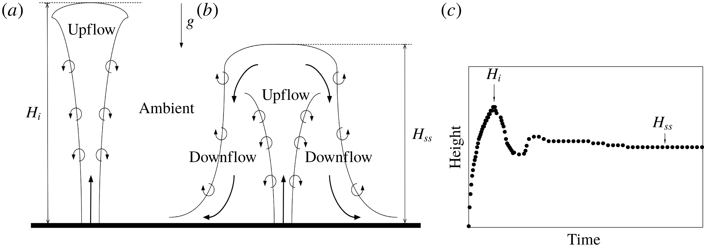
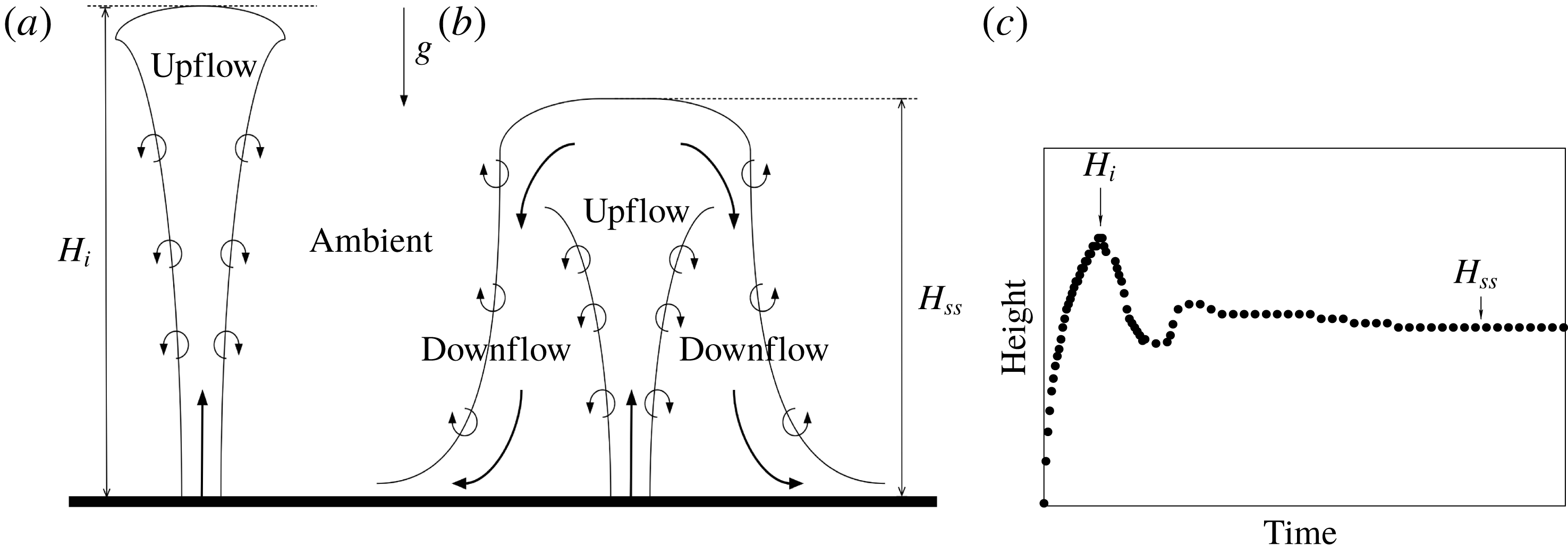
As depicted in figure 1(a), during its initial transient phase, the momentum of a fountain competes with the opposite buoyancy until the fountain reaches a null vertical velocity at a maximum initial height
 $H_{i}$
. Then, at this height, an annular downflow settles with a density higher than the ambient and surrounds the upflow. A steady state is then reached and the penetration height of the fountain stabilizes at a value
 $H_{ss}$
generally lower than the initial value
 $H_{i}$
(see figure 1
b). The typical time evolution of the fountain is depicted in figure 1(c).
In the present study, we shall distinguish between upward and downward fountains: upward (respectively downward) fountains refer to the release of a fluid in a lighter (respectively heavier) ambient. In the literature, many experiments focusing either on upward fountains (Turner Reference Turner1966; Baines et al. Reference Baines, Turner and Campbell1990; Pantzlaff & Lueptow Reference Pantzlaff and Lueptow1999; Burridge & Hunt Reference Burridge and Hunt2012) or on downward fountains (Seban, Behnia & Abreu Reference Seban, Behnia and Abreu1978; Cresswell & Szczepura Reference Cresswell and Szczepura1993; Papanicolaou & Kokkalis Reference Papanicolaou and Kokkalis2008) have been realized. These experiments were all carried out for modest density contrasts between the ambient and the release, i.e. for so-called Boussinesq fountains. For such fountains, when the conditions at the source are similar (in terms of volume, momentum and buoyancy fluxes), there are no differences between the penetration heights of an upward fountain and those of a downward fountain. Thus, the question is whether some differences might be observed in the case of significant density contrasts between the ambient and the release, i.e. for so-called non-Boussinesq fountains. This is the aim of the present paper.
The paper is organized as follows. In § 2, some of the fundamentals of turbulent fountains are presented. Our numerical model is described in § 3. The results of the simulations are presented and discussed in § 4. Finally, conclusions are offered in § 5.
2 Fundamentals of turbulent fountains
Sketch of the (a) initial upflow and (b) steady state of a turbulent fountain during (c) the corresponding typical time evolution of the penetration height.
As a pioneering work, Turner (Reference Turner1966) studied experimentally and theoretically the reversing buoyant jets and plumes for the special case of cumulus clouds. Based on a dimensional analysis considering both buoyancy and momentum fluxes, one of Turner’s main results is the linear scaling of the steady dimensionless height
 $H_{ss}/b_{i}$
with the Boussinesq source Froude number
 $Fr$
:
 $$\begin{eqnarray}Fr=\frac{w_{i}}{\sqrt{g\unicode[STIX]{x1D702}_{i}b_{i}}},\end{eqnarray}$$
where
 $g$
is the gravitational acceleration and
 $w_{i}$
,
 $b_{i}$
and
 $\unicode[STIX]{x1D702}_{i}$
are respectively the velocity, the radius and the relative density difference of the discharge at the source location. The density deficit is defined by
 $\unicode[STIX]{x1D702}_{i}=|\unicode[STIX]{x1D70C}_{i}-\unicode[STIX]{x1D70C}_{0}|/\unicode[STIX]{x1D70C}_{0}$
, where
 $\unicode[STIX]{x1D70C}_{i}$
is the source density of the release and
 $\unicode[STIX]{x1D70C}_{0}$
that of the ambient. By widening the range of Froude numbers (
 $0.56\lesssim Fr\lesssim 11.8$
) studied by Turner (Reference Turner1966) to larger values of
 $Fr$
, many other experimental works (including Seban et al.
Reference Seban, Behnia and Abreu1978; Baines et al.
Reference Baines, Turner and Campbell1990; Cresswell & Szczepura Reference Cresswell and Szczepura1993; Zhang & Baddour Reference Zhang and Baddour1998; Pantzlaff & Lueptow Reference Pantzlaff and Lueptow1999; Kaye & Hunt Reference Kaye and Hunt2006) confirmed the linear scaling
 $H_{ss}/b_{i}\propto Fr$
for large source Froude numbers (
 $Fr\gtrsim 3$
) with a constant of proportionality lying between
 $2.10$
and
 $2.46$
.
Also of interest is the initial rise of the fountain up to its maximum initial height
 $H_{i}$
. Extending the original theoretical work of Morton, Taylor & Turner (Reference Morton, Taylor and Turner1956) to forced plumes with negative buoyancy, Morton (Reference Morton1959) demonstrated that the dimensionless height
 $H_{i}/b_{i}$
is also proportional to the source Froude number
 $Fr$
. As a consequence, the ratio
 $\unicode[STIX]{x1D706}=H_{i}/H_{ss}$
turns out to be a constant: both experiments (Turner Reference Turner1966; Pantzlaff & Lueptow Reference Pantzlaff and Lueptow1999; Burridge & Hunt Reference Burridge and Hunt2012) and theoretical works (Bloomfield & Kerr Reference Bloomfield and Kerr2000; Mehaddi et al.
Reference Mehaddi, Vaux, Candelier and Vauquelin2015b
) have found
 $\unicode[STIX]{x1D706}\sim 1.43$
for values of the source Froude number larger than
 $5.5$
. For lower values of the source Froude number and based on the evolution of
 $H_{ss}/b_{i}$
and
 $\unicode[STIX]{x1D706}$
with
 $Fr$
, the need for a classification of the Boussinesq turbulent axisymmetric fountains appeared within the works of Zhang & Baddour (Reference Zhang and Baddour1998) and Kaye & Hunt (Reference Kaye and Hunt2006). Zhang & Baddour (Reference Zhang and Baddour1998) identified two regimes, weak and forced, and Kaye & Hunt (Reference Kaye and Hunt2006) added a third regime (very weak). Recently, Burridge & Hunt (Reference Burridge and Hunt2012) proposed in their experimental work a more detailed classification into five regimes according to the value of the source Froude number
 $Fr$
: very weak (
 $Fr\lesssim 1.0$
), weak (
 $1.0\lesssim Fr\lesssim 1.7$
), intermediate (
 $1.7\lesssim Fr\lesssim 2.8$
), forced (
 $2.8\lesssim Fr\lesssim 5.5$
) and highly forced (
 $Fr\gtrsim 5.5$
). Each class encompasses a steady height dependency on
 $Fr$
and a range of
 $\unicode[STIX]{x1D706}$
. Burridge & Hunt (Reference Burridge and Hunt2012) also showed that the rise height ratio
 $\unicode[STIX]{x1D706}$
is found to be constant,
 $\unicode[STIX]{x1D706}=1.45$
, only for the highly forced regime and could decrease down to
 $1.0$
for the forced regime. However, for both the forced and highly forced regime, Burridge & Hunt (Reference Burridge and Hunt2012) confirmed the linear scaling by Turner (Reference Turner1966) which reads
 $$\begin{eqnarray}H_{ss}/b_{i}=2.46Fr.\end{eqnarray}$$
In comparison with experimental works, numerical simulations of turbulent fountains are more scarce in the literature. Recently, we note the studies by direct numerical simulations of very weak and weak fountains over the range
 $0.1\leqslant Fr\leqslant 2.1$
by Williamson, Armfield & Lin (Reference Williamson, Armfield and Lin2010) and the forced fountain flow regime for
 $Fr=4$
and
 $7$
by Williamson, Armfield & Lin (Reference Williamson, Armfield and Lin2011). In the latter, the steady penetration height of the fountains is found to collapse on the
 $H_{ss}/b_{i}=2.46Fr$
curve. In addition, the morphology of the fountain is highlighted, as well as a detailed description of the dynamics of the flow. In the recent theoretical work of Mehaddi et al. (Reference Mehaddi, Vaux, Candelier and Vauquelin2015b
), inspired by Carazzo, Kaminski & Tait (Reference Carazzo, Kaminski and Tait2010), high-Froude-number turbulent fountains are considered and a model accounting for the effect of the downflow on the fountain upflow is derived. In order to determine the constants of the model, this work is supported by large-eddy simulations. Again, the model allows the relation
 $H_{ss}/b_{i}=2.46Fr$
and the ratio
 $\unicode[STIX]{x1D706}=1.43$
to be recovered.
All the mentioned studies (experimental, theoretical or numerical) have considered the Boussinesq approximation and have been carried out for upward or downward fountains. In all the cases, we do not notice any difference in the correlations.
Actually, unlike the Boussinesq case, negatively non-Boussinesq buoyant releases have received much less attention. We only note the works of Baddour & Zhang (Reference Baddour and Zhang2009) and Mehaddi, Vauquelin & Candelier (Reference Mehaddi, Vauquelin and Candelier2015a
). Baddour & Zhang (Reference Baddour and Zhang2009) studied experimentally round hypersaline upward turbulent fountains in the highly forced regime over the range
 $Fr=7.6-45.6$
and a relative density difference variation,
 $\unicode[STIX]{x0394}\unicode[STIX]{x1D70C}/\unicode[STIX]{x1D70C}_{0}=0.001-0.1$
. They measured the penetration height and obtained a relation
 $H_{ss}/b_{i}=f(\unicode[STIX]{x0394}\unicode[STIX]{x1D70C}/\unicode[STIX]{x1D70C}_{0})Fr$
with
 $f(\unicode[STIX]{x0394}\unicode[STIX]{x1D70C}/\unicode[STIX]{x1D70C}_{0})$
approximately equal to a constant for
 $\unicode[STIX]{x0394}\unicode[STIX]{x1D70C}/\unicode[STIX]{x1D70C}_{0}\leqslant 0.003$
before monotonically declining by 15 % at the maximum for
 $\unicode[STIX]{x0394}\unicode[STIX]{x1D70C}/\unicode[STIX]{x1D70C}_{0}=0.1$
. The recent experimental work by Mehaddi et al. (Reference Mehaddi, Vauquelin and Candelier2015a
) focuses on downward air–helium fountains in ambient air over a wide range of density ratio
 $0.13<\unicode[STIX]{x1D70C}_{i}/\unicode[STIX]{x1D70C}_{0}<0.96$
and Froude number
 $0.2<Fr<64$
. These authors extend the classical Boussinesq height
 $H_{ss}$
correlations provided that the (Boussinesq) Froude number
 $Fr$
is multiplied by
 $(\unicode[STIX]{x1D70C}_{i}/\unicode[STIX]{x1D70C}_{0})^{1/2}$
. As previously used by several authors (Crapper & Baines (Reference Crapper and Baines1978), Michaux & Vauquelin (Reference Michaux and Vauquelin2008) for plumes and Mehaddi et al. (Reference Mehaddi, Vauquelin and Candelier2015a
) for fountains), the following generalized (non-Boussinesq) Froude number
 $Fr_{NB_{d}}$
is introduced:
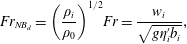 $$\begin{eqnarray}Fr_{NB_{d}}=\left(\displaystyle \frac{\unicode[STIX]{x1D70C}_{i}}{\unicode[STIX]{x1D70C}_{0}}\right)^{1/2}Fr=\frac{w_{i}}{\sqrt{g\unicode[STIX]{x1D702}_{i}^{\prime }b_{i}}},\end{eqnarray}$$
where
 $\unicode[STIX]{x1D702}_{i}^{\prime }=(\unicode[STIX]{x1D70C}_{0}-\unicode[STIX]{x1D70C}_{i})/\unicode[STIX]{x1D70C}_{i}$
is the density difference relative to the source density
 $\unicode[STIX]{x1D70C}_{i}$
. By plotting the experimental steady state height
 $H_{ss}/b_{i}$
as a function of the non-Boussinesq Froude number
 $Fr_{NB_{d}}$
, they find a linear relation,
 $H_{ss}/b_{i}=2.58Fr_{NB_{d}}$
(note that the form of the relation is similar to the Boussinesq situation, where the Boussinesq Froude number
 $Fr$
has been replaced by the downward non-Boussinesq Froude number
 $Fr_{NB_{d}}$
and the proportionality constant
 $2.46$
by
 $2.58$
). However, in the appendix of their paper, they show that if we consider the classical correction of the entrainment coefficient
 $\unicode[STIX]{x1D6FC}$
for the non-Boussinesq plumes (Ricou & Spalding Reference Ricou and Spalding1961; Rooney & Linden Reference Rooney and Linden1996; Michaux & Vauquelin Reference Michaux and Vauquelin2008; Van den Bremer & Hunt Reference Van den Bremer and Hunt2010), the Froude number has to be multiplied by a density ratio (
 $\unicode[STIX]{x1D70C}_{i}/\unicode[STIX]{x1D70C}_{0}$
) exhibiting an exponent greater than
 $1/2$
, namely
 $3/4$
. We can therefore imagine that some non-Boussinesq effects can modify the nature of the correlations following the direction of injection (upwards or downwards). To answer this question and to extend the results of Mehaddi et al. (Reference Mehaddi, Vauquelin and Candelier2015a
), numerical simulations are carried out for both downward and upward non-Boussinesq fountains. These numerical simulations are described in the following section.
3 Numerical simulations
We consider vertical, isothermal and continuous releases of gas mixtures to simulate downward and upward non-Boussinesq turbulent miscible fountains. For the downward case, simulations have been carried out for a density ratio
 $\unicode[STIX]{x1D70C}_{i}/\unicode[STIX]{x1D70C}_{0}$
ranging from 0.05 to 0.8. For the upward case, the density contrast varies between
 $1.52$
and
 $12$
. A total of around forty simulations were achieved over the range
 $4.0\lesssim Fr\lesssim 29$
corresponding originally to the forced or highly forced Boussinesq regime. In all the simulations, the Reynolds number based on the source diameter is set to
 $Re=4000$
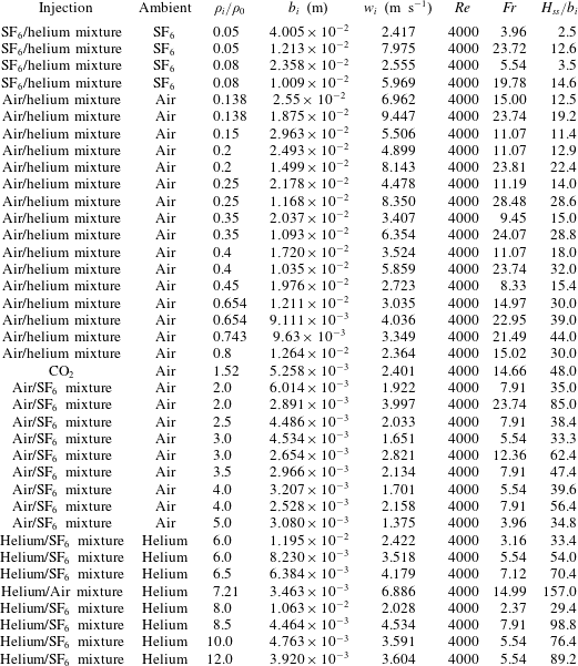
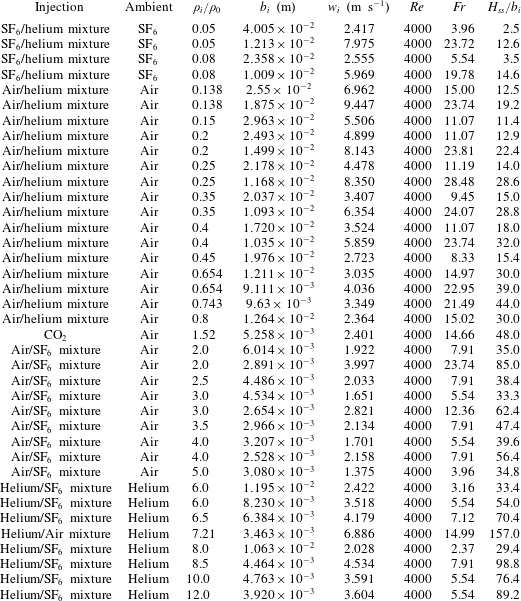
(see table 2 in appendix C for the source parameters of the fountain simulations).
To simulate numerically a turbulent fountain, we use large-eddy simulations to solve the Favre-filtered Navier–Stokes equations (mass and momentum balance) along with species transport equations. We use the numerical computational code CALIF
 $^{3}$
S-ISIS (software developed at the French Institut de Radioprotection et de Sûreté Nucléaire (IRSN)), dedicated to three-dimensional simulations of turbulent and slightly compressible flows (low-Mach-number approach). The three-dimensional filtered Navier–Stokes equations in Cartesian coordinates are as follows:
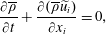 $$\begin{eqnarray}\displaystyle & \displaystyle \frac{\unicode[STIX]{x2202}\overline{\unicode[STIX]{x1D70C}}}{\unicode[STIX]{x2202}t}+\frac{\unicode[STIX]{x2202}(\overline{\unicode[STIX]{x1D70C}}\widetilde{u_{i}})}{\unicode[STIX]{x2202}x_{i}}=0, & \displaystyle\end{eqnarray}$$
 $$\begin{eqnarray}\displaystyle & \displaystyle \frac{\unicode[STIX]{x2202}(\overline{\unicode[STIX]{x1D70C}}\widetilde{u_{i}})}{\unicode[STIX]{x2202}t}+\frac{\unicode[STIX]{x2202}(\overline{\unicode[STIX]{x1D70C}}\widetilde{u_{i}}\widetilde{u_{j}})}{\unicode[STIX]{x2202}x_{j}}=-\frac{\unicode[STIX]{x2202}\overline{p}}{\unicode[STIX]{x2202}x_{i}}+\frac{\unicode[STIX]{x2202}\overline{\unicode[STIX]{x1D61A}}_{ij}}{\unicode[STIX]{x2202}x_{j}}+(\unicode[STIX]{x1D70C}_{0}-\overline{\unicode[STIX]{x1D70C}})g_{i}-\frac{\unicode[STIX]{x2202}\unicode[STIX]{x1D70F}_{ij}}{\unicode[STIX]{x2202}x_{j}}, & \displaystyle\end{eqnarray}$$
where
 $\widetilde{u_{i}}$
is the Favre-filtered velocity and
 $\overline{p}$
is the dynamic pressure. The density
 $\overline{\unicode[STIX]{x1D70C}}$
is the filtered density of the fluid and is calculated using the ideal gas law in combination with the mass fraction of the different species of the gas mixture. In (3.2),
 $g_{i}$
is the gravitational acceleration,
 $\unicode[STIX]{x1D70F}_{ij}=\overline{\unicode[STIX]{x1D70C}u_{i}u_{j}}-\overline{\unicode[STIX]{x1D70C}}\widetilde{u_{i}}\widetilde{u_{j}}$
represents the subgrid-scale Reynolds stress and
 $\overline{\unicode[STIX]{x1D61A}}_{ij}=-(2/3)\unicode[STIX]{x1D707}(\unicode[STIX]{x2202}\widetilde{u_{k}}/\unicode[STIX]{x2202}x_{k})\unicode[STIX]{x1D6FF}_{ij}+\unicode[STIX]{x1D707}(\unicode[STIX]{x2202}\widetilde{u_{i}}/\unicode[STIX]{x2202}x_{j}+\unicode[STIX]{x2202}\widetilde{u_{j}}/\unicode[STIX]{x2202}x_{i})$
is the filtered strain rate tensor where
 $\unicode[STIX]{x1D707}$
is the molecular dynamic viscosity calculated as a function of the individual viscosities and molar masses as well as the corresponding mass fractions.
The mass fraction
 $y_{k}$
of a species
 $k$
is governed by a species transport equation which reads as:
 $$\begin{eqnarray}\frac{\unicode[STIX]{x2202}\overline{\unicode[STIX]{x1D70C}}\widetilde{y_{k}}}{\unicode[STIX]{x2202}t}+\frac{\unicode[STIX]{x2202}(\overline{\unicode[STIX]{x1D70C}}\widetilde{y_{k}}\widetilde{u_{i}})}{\unicode[STIX]{x2202}x_{i}}=\frac{\unicode[STIX]{x2202}}{\unicode[STIX]{x2202}x_{i}}\left(\overline{\unicode[STIX]{x1D70C}}D\frac{\unicode[STIX]{x2202}\widetilde{y_{k}}}{\unicode[STIX]{x2202}x_{i}}+\frac{\unicode[STIX]{x1D707}_{t}}{Sc_{t}}\frac{\unicode[STIX]{x2202}\widetilde{y_{k}}}{\unicode[STIX]{x2202}x_{i}}\right),\end{eqnarray}$$
where
 $\widetilde{y_{k}}$
stands for the Favre-filtered mass fraction of the
 $k$
th component of the mixture and
 $D$
represents the molecular diffusivity of the mixture. In (3.3), the simple gradient diffusion hypothesis (SGDH) is used to close the problem with a turbulent Schmidt number
 $Sc_{t}$
set to
 $0.7$
. In the simulations, a box filter in each direction is implicitly applied and the WALE (wall adapting local eddy) subgrid-scale model for the subgrid Reynolds stress (Nicoud & Ducros Reference Nicoud and Ducros1999) is adopted. A staggered grid is used with a cell-centred piecewise constant representation of the scalar variables and with a marker and cell (MAC) type finite volume approximation for the velocity. For the time discretization, we use a fractional step algorithm decoupling balance equations for the transport of species and Navier–Stokes equations which are solved by a pressure correction technique. As we consider fountains in an infinite (open) environment, the computational domain must be bounded by artificial boundary conditions which perturb as little as possible the flow in the interior of the domain. The boundary conditions used in our simulations are based on the usual control of the kinetic energy and allow us to distinguish between the flow that leaves the domain and the flow that enters it. This type of boundary condition was initially established for the incompressible case in Bruneau & Fabrie (Reference Bruneau and Fabrie1994, Reference Bruneau and Fabrie1996) and its extension to compressible flows was tackled in Bruneau (Reference Bruneau2000).
The three-dimensional computational domains
 $\unicode[STIX]{x1D6FA}$
are rectangular boxes. In each simulation, the values set to the total lateral
 $l$
and vertical
 $L$
lengths depend on the physical parameters of the flow under consideration (see appendix A for more detail). The source is set flush with the bottom (respectively the top) solid boundary of the computational domain
 $\unicode[STIX]{x1D6FA}$
for an upward (respectively downward) injection and the fountain emerges at the centre of
 $\unicode[STIX]{x1D6FA}$
. We use a refined Cartesian grid with a uniform square mesh (
 $\unicode[STIX]{x0394}x\times \unicode[STIX]{x0394}y$
) over a subregion
 $\unicode[STIX]{x1D6FA}_{1}$
centred at the origin. Outside
 $\unicode[STIX]{x1D6FA}_{1}$
, the grid is stretched toward the lateral boundaries of the domain. In the vertical direction
 $z$
, the grid spacing (i.e.
 $\unicode[STIX]{x0394}z$
) is kept uniform from the source vertical position up to a vertical distance
 $L_{1z}$
and then stretched toward the opposite boundary. To initiate the turbulence at the source, we apply an azimuthal forcing similar to Zhou, Luo & Williams (Reference Zhou, Luo and Williams2001).
For each simulated case, a grid convergence study was carried out to validate the box length
 $l$
, the domain height
 $L$
, the extent of the subregions
 $\unicode[STIX]{x1D6FA}_{1}$
and
 $L_{1z}$
and the grid spacing in each direction. We tested vertical grid spacings
 $\unicode[STIX]{x0394}z/b_{i}$
ranging from
 $0.4$
to
 $0.125$
and horizontal grid spacings
 $\unicode[STIX]{x0394}x/b_{i}$
varying from
 $0.2$
to
 $0.067$
. For the time discretization, a CFL (Courant–Friedrichs–Lewy) number close to unity has been imposed for each calculation even if time step sizes for which CFL numbers greater than one are allowed with the use of implicit schemes. We set the duration times of the simulations sufficiently large to guarantee first that the steady states of the fountains are reached and secondly to ensure the convergence of the time-averaged values of the fountain variables (the variations of the mean field fall below 3 % of the value of the mean). In practice, the time interval over which the statistics were computed covers approximately 20 fountain-oscillation periods (see Mehaddi et al.
Reference Mehaddi, Vaux, Candelier and Vauquelin2015b
).
Furthermore, a previous simulation presented in Mehaddi et al. (Reference Mehaddi, Vaux, Candelier and Vauquelin2015b
) in comparison with the experiment by Cresswell & Szczepura (Reference Cresswell and Szczepura1993) (hot water injected into a tank of fresh water with
 $Re=5000$
and
 $Fr=3.1$
) has been repeated in order to verify the ability of the large-eddy simulation (LES) approach to reproduce a turbulent miscible fountain. By simulating the equivalent downwards injection of hot air into cold ambient air, it has been shown that the computed time-averaged (radial) profiles of velocity, Reynolds stress and density deficit compare well with the experimental data. We will see further in the paper that the results of Mehaddi et al. (Reference Mehaddi, Vauquelin and Candelier2015a
) for the steady state height
 $H_{ss}/b_{i}$
of downward non-Boussinesq turbulent fountains are also recovered by our simulations, confirming the suitability of the CALIF
 $^{3}$
S-ISIS code to properly evaluate the heights of non-Boussinesq fountains.
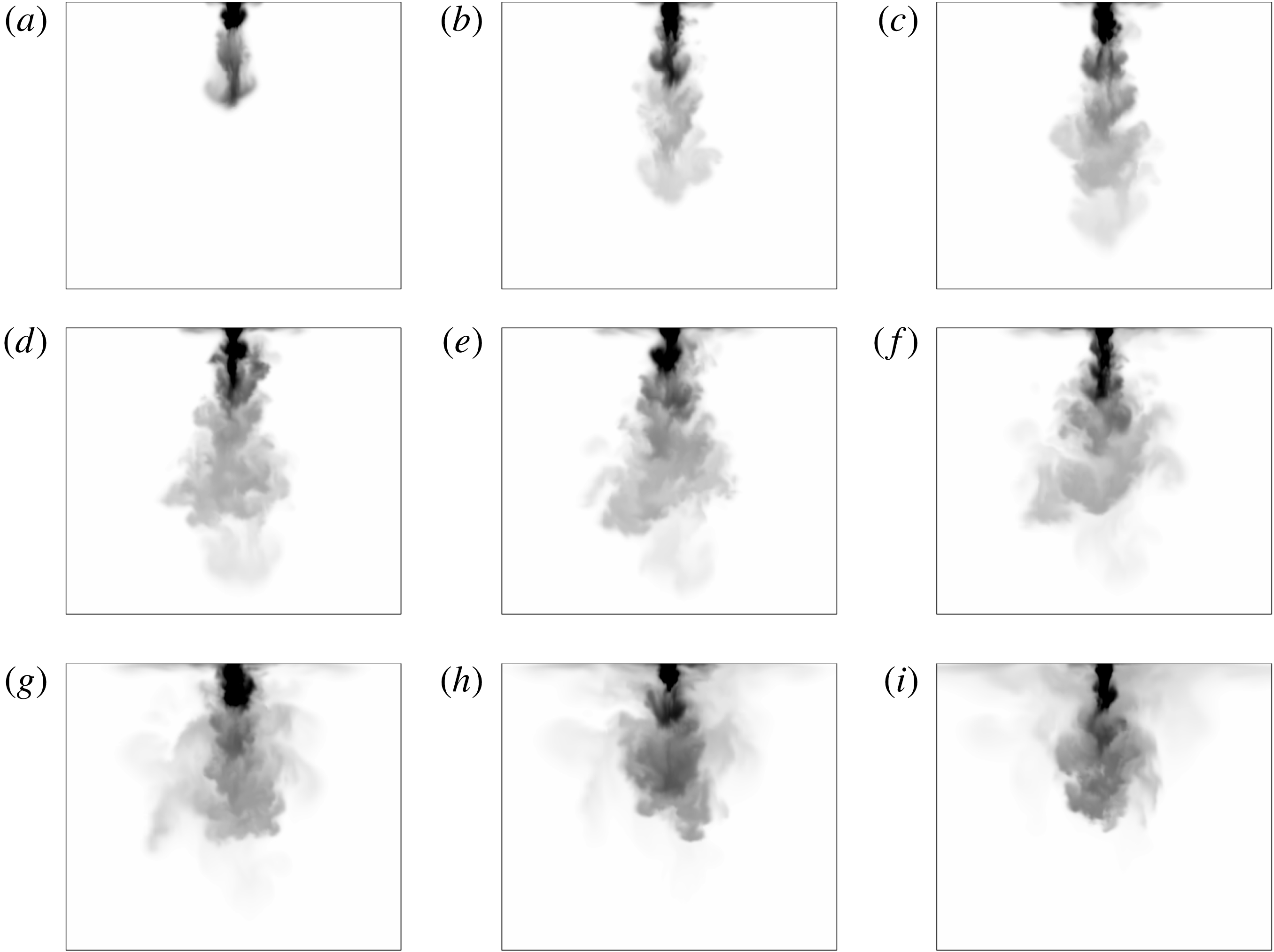
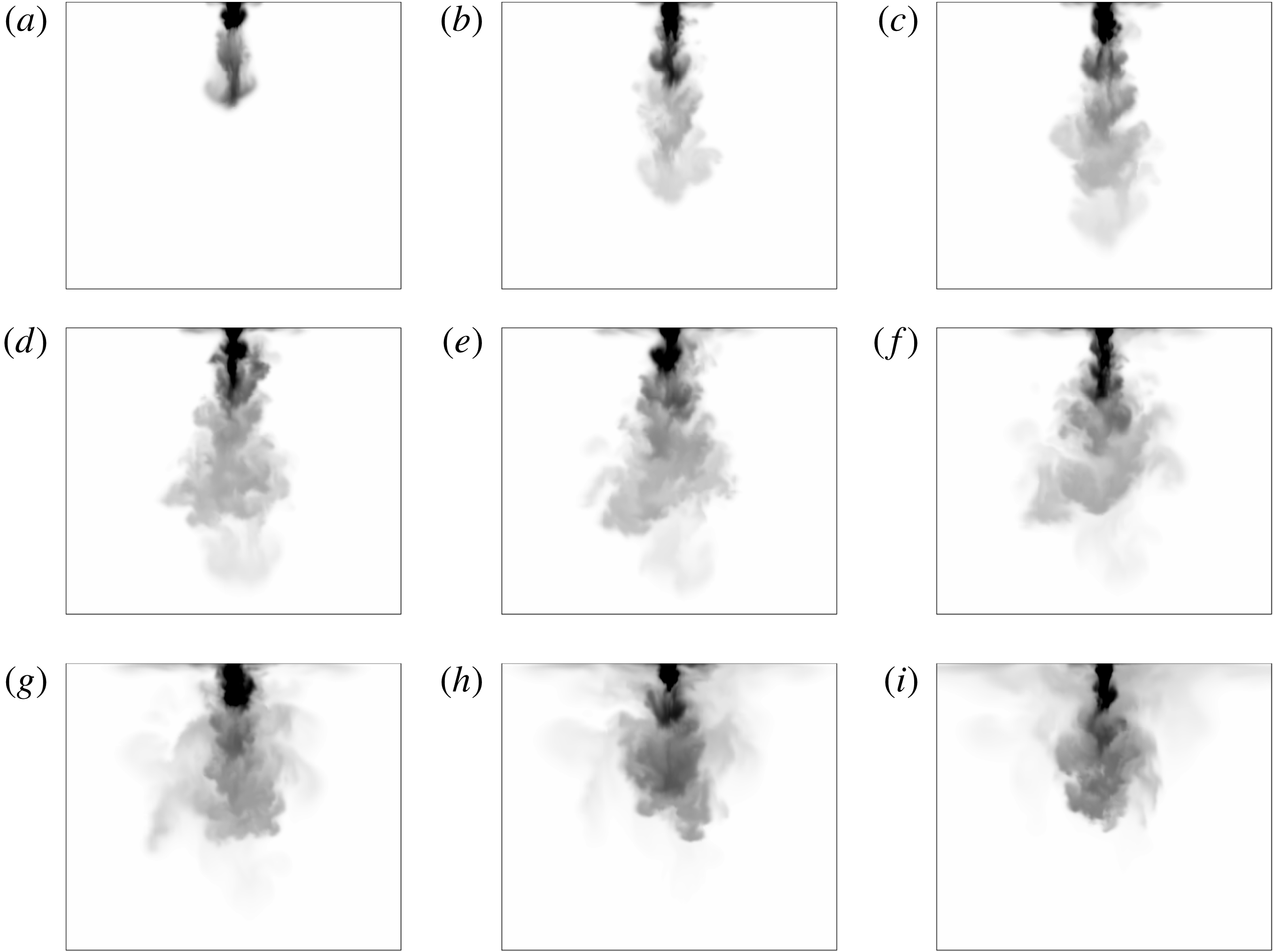
As an illustration of the flow development, figure 2 presents successive snapshots of a downward fountain.
Flow development of a downward non-Boussinesq fountain with
 $Fr=23.7,\unicode[STIX]{x1D70C}_{i}/\unicode[STIX]{x1D70C}_{0}=0.4$
from
 $t=0.15~\text{s}$
(a) with an increment of
 $\unicode[STIX]{x1D6FF}t=0.30~\text{s}$
between each snapshot.
4 Results and discussion
4.1 Fountain heights
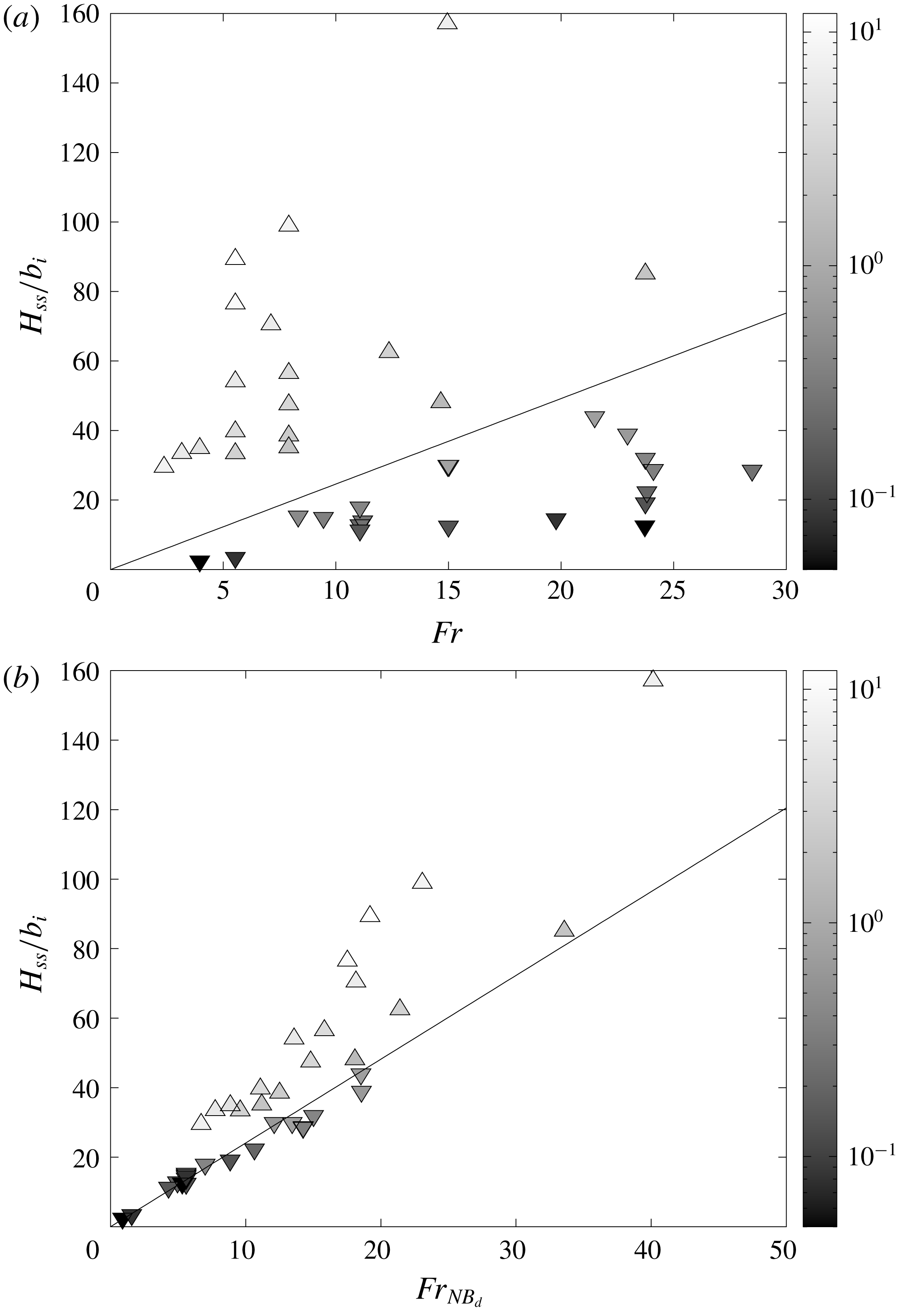
Figure 3(a) shows, for the whole set of upward and downward simulations, the steady state heights
 $H_{ss}/b_{i}$
of the fountain as a function of the source Froude number
 $Fr$
together with the relation
 $H_{ss}/b_{i}=2.46Fr$
(valid for the Boussinesq case). In this figure, upward (respectively downward) triangles are related to upward (respectively downward) fountains and a grey scale colour bar is adopted to indicate the value of the density ratio over the range
 $\unicode[STIX]{x1D70C}_{i}/\unicode[STIX]{x1D70C}_{0}=0.05$
to
 $12$
(dark grey for
 $\unicode[STIX]{x1D70C}_{i}/\unicode[STIX]{x1D70C}_{0}\ll 1$
and light grey for
 $\unicode[STIX]{x1D70C}_{i}/\unicode[STIX]{x1D70C}_{0}\gg 1$
). For density ratios far from the Boussinesq approximation, we notice a strong deviation from the so-called Boussinesq relation (2.2) indicating that
 $\unicode[STIX]{x1D70C}_{i}/\unicode[STIX]{x1D70C}_{0}$
has a marked influence on the steady state height
 $H_{ss}$
. In figure 3(a), the Boussinesq relation is found to clearly separate the downward and upward cases. Dispersion of the data does not suggest any simple correlation in Froude number but raises a clear dependence with
 $\unicode[STIX]{x1D70C}_{i}/\unicode[STIX]{x1D70C}_{0}$
for both situations.
(a) Comparison between the present numerical results for the dimensionless fountain height
 $H_{ss}/b_{i}$
and the correlation (solid line),
 $H_{ss}/b_{i}=2.46Fr$
. The data points, (▵) for upward fountains and (▿) for downward fountains, are shaded according to the density ratio
 $\unicode[STIX]{x1D70C}_{i}/\unicode[STIX]{x1D70C}_{0}$
. (b) Comparison between the present numerical results (symbols similar to figure 3
a) for the dimensionless fountain height
 $H_{ss}/b_{i}$
and the correlation (solid line),
 $H_{ss}/b_{i}=2.41Fr_{NB_{d}}$
.

In the light of this experimental finding, we plot in figure 3(b) the downward and upward simulation results for the steady height
 $H_{ss}/b_{i}$
in terms of the non-Boussinesq Froude number
 $Fr_{NB_{d}}$
. For the downward case, the data collapse onto a unique curve given by the linear scaling (4.1):
 $$\begin{eqnarray}H_{ss}/b_{i}=2.41Fr_{NB_{d}}\quad \text{for }\unicode[STIX]{x1D70C}_{i}/\unicode[STIX]{x1D70C}_{0}<1.\end{eqnarray}$$
We recover (with a 7 % difference on the value of the coefficient) the experimental correlation obtained from the measurements of air–helium fountain heights of Mehaddi et al. (Reference Mehaddi, Vauquelin and Candelier2015a ). We underline that this agreement constitutes a reliable validation criterion of our simulations.
By contrast, it is striking to note that the points for the steady height
 $H_{ss}/b_{i}$
corresponding to an upward release still keep away from the linear relation (4.1). Thus, a first and noteworthy feature is that upward and downward non-Boussinesq turbulent fountains are not similar as observed in Boussinesq situations where the direction of injection does not matter and a unique relation
 $H_{ss}/b_{i}\propto Fr$
is found. A second feature is that whereas the quantity
 $b_{i}Fr_{NB_{d}}$
is a suitable length scale for downward non-Boussinesq fountains, this quantity is not relevant for the upward case.
We can rewrite the linear relation (4.1) for downward non-Boussinesq fountains in order to highlight the power-law dependence of the steady height
 $H_{ss}$
with the density ratio
 $\unicode[STIX]{x1D70C}_{i}/\unicode[STIX]{x1D70C}_{0}$
:
 $$\begin{eqnarray}\frac{H_{ss}}{2.46b_{i}Fr}\simeq 0.98\left(\frac{\unicode[STIX]{x1D70C}_{i}}{\unicode[STIX]{x1D70C}_{0}}\right)^{1/2}\quad \text{for }\unicode[STIX]{x1D70C}_{i}/\unicode[STIX]{x1D70C}_{0}<1.\end{eqnarray}$$
The idea is now to examine the behaviour of the quantity
 $H_{ss}/(2.46b_{i}Fr)$
as a function of the density ratio
 $\unicode[STIX]{x1D70C}_{i}/\unicode[STIX]{x1D70C}_{0}$
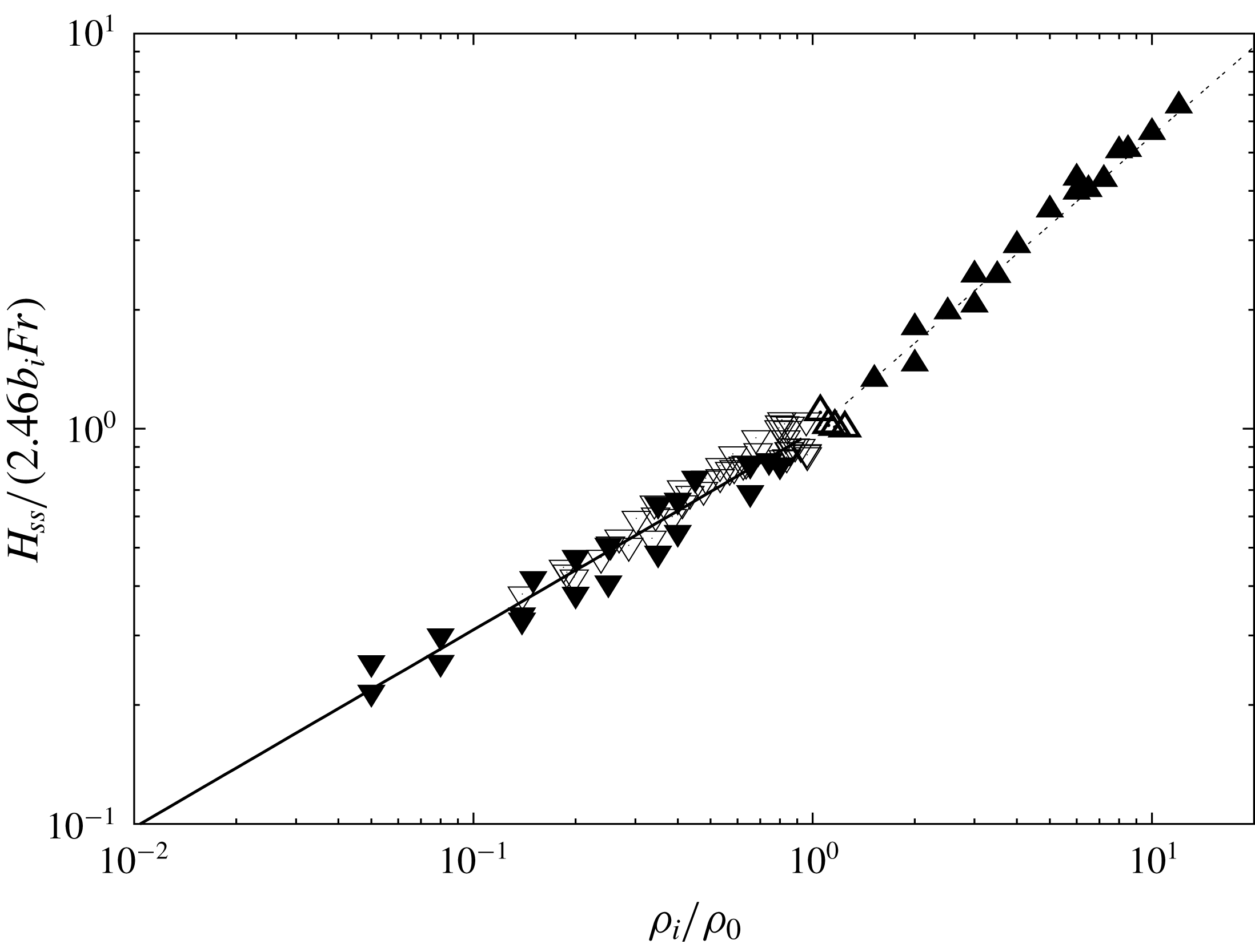
for the whole set of simulations. The result is plotted in figure 4 as well as the more appropriate power law for the density ratio for each direction of injection. In addition to the relation (4.2) obtained for downward fountains, a second power-law behaviour with the density ratio
 $\unicode[STIX]{x1D70C}_{i}/\unicode[STIX]{x1D70C}_{0}$
can be clearly observed for the upward fountains:
 $$\begin{eqnarray}\frac{H_{ss}}{2.46b_{i}Fr}\simeq 0.98\left(\frac{\unicode[STIX]{x1D70C}_{i}}{\unicode[STIX]{x1D70C}_{0}}\right)^{3/4}\quad \text{for }\unicode[STIX]{x1D70C}_{i}/\unicode[STIX]{x1D70C}_{0}>1.\end{eqnarray}$$
Unlike the downward injection, the trend of the steady height
 $H_{ss}/(2.46b_{i}Fr)$
for the upward fountains dramatically changes to adopt a
 $(\unicode[STIX]{x1D70C}_{i}/\unicode[STIX]{x1D70C}_{0})^{3/4}$
behaviour.
Normalized fountain height (
 $H_{ss}/(2.46b_{i}Fr)$
) plotted against the density ratio (
 $\unicode[STIX]{x1D70C}_{i}/\unicode[STIX]{x1D70C}_{0}$
) where ▵ represent experimental data for upward fountains by Baddour & Zhang (Reference Baddour and Zhang2009), ▿ are experimental data for downward fountains by Mehaddi et al. (Reference Mehaddi, Vauquelin and Candelier2015a
), (▴) correspond to our simulations of upward fountains and (▾) of downward fountains. The solid line represents the power law of the density ratio for the downward case, with a slope of
 $1/2$
and the dash-dotted line represents the power law of the density ratio for the upward case, with a slope of
 $3/4$
.

This trend demonstrates the asymmetry of non-Boussinesq fountains with respect to the direction of injection. Actually, a similar non-Boussinesq asymmetry can be found in the Rayleigh–Bénard literature (see for instance Wu & Libchaber Reference Wu and Libchaber1991). In Rayleigh–Bénard convection, asymmetry can be explained by the fact that the physical properties of the fluid vary with temperature. In our simulations, however, the fountains are isothermal and therefore their physical properties are constant. The only mechanism that explains the asymmetry between downward and upward fountains is the mixing process. As discussed by Bloomfield & Kerr (Reference Bloomfield and Kerr2000), the entrainment process in a steady turbulent fountain is due to the return flow that entrains the surrounding fluid as a line plume. It is indeed widely accepted that the ambient fluid is entrained by vortices at the edge of the fountain. The mixing process can be attributed to two distinct effects, namely the shear and the baroclinic torque (Kaye Reference Kaye2008). There is no reason for the contribution of the shear to be different for an upward fountain and for a downward fountain. In contrast, the contribution of the baroclinic torque to the entrainment process will be of opposite sign depending on the considered configuration (see Hermanson & Cetegen Reference Hermanson and Cetegen2000). The physical reasons why upward non-Boussinesq fountains differ from downward non-Boussinesq fountains are based on this contribution, with values of the baroclinic torque depending on the large density difference but with an opposite sign according to the direction of injection. For Boussinesq fountains where the density deficit is small, the contribution of the baroclinic torque to the entrainment process turns out to be too weak to observe an asymmetry.
As already mentioned, the relation (4.1) (as with that obtained experimentally in Mehaddi et al. (Reference Mehaddi, Vauquelin and Candelier2015a
)) obtained for a downward release should be seen as the equivalent to the relation
 $H_{ss}/b_{i}=2.46Fr$
obtained for turbulent Boussinesq fountains. In the case of an upward injection, such a comparison is not straightforward. Nevertheless, if we define a modified radius
 $\unicode[STIX]{x1D6FD}=(\unicode[STIX]{x1D70C}_{i}/\unicode[STIX]{x1D70C}_{0})^{1/2}b_{i}$
and an upward non-Boussinesq Froude number
 $Fr_{NB_{u}}$
based on the modified radius
 $\unicode[STIX]{x1D6FD}$
and defined by:
 $$\begin{eqnarray}Fr_{NB_{u}}=\left(\frac{\unicode[STIX]{x1D70C}_{i}}{\unicode[STIX]{x1D70C}_{0}}\right)^{1/4}Fr=\frac{w_{i}}{\sqrt{g\unicode[STIX]{x1D702}_{i}^{\prime }\unicode[STIX]{x1D6FD}}},\end{eqnarray}$$
(4.3) can be recast into the form:
 $$\begin{eqnarray}H_{ss}/\unicode[STIX]{x1D6FD}=2.41Fr_{NB_{u}}.\end{eqnarray}$$
As a result, the relation (4.5) for upward non-Boussinesq fountains appears as the equivalent of (4.1) and (2.2) for respectively downward non-Boussinesq fountains and Boussinesq fountains. Note that as a consequence of the linear scaling laws (4.1) and (4.5), the quantities
 ${\mathcal{L}}_{d}=b_{i}Fr_{NB_{d}}$
and
 ${\mathcal{L}}_{u}=\unicode[STIX]{x1D6FD}Fr_{NB_{u}}$
may be seen as appropriate characteristic length scales for respectively downward and upward non-Boussinesq forced fountains.
4.2 Length and time scales
The question now arises whether the scaling observed for the steady height can be extended to the whole time history of the fountain penetration height. In the present context of turbulent forced fountains, where the flow is dominated by momentum and buoyancy fluxes, we recall that characteristic length scales can be defined in the basis
 $(M_{i},B_{i})$
(Turner Reference Turner1966; Baines et al.
Reference Baines, Turner and Campbell1990; Burridge & Hunt Reference Burridge and Hunt2012) where
 $M_{i}$
and
 $B_{i}$
are respectively the source fluxes of momentum and buoyancy. For a Boussinesq release, the source fluxes of momentum,
 $M_{i}$
, and buoyancy,
 $B_{i}$
, are defined respectively by:
 $$\begin{eqnarray}M_{i}=2\unicode[STIX]{x03C0}\int _{0}^{b_{i}}\overline{w}^{2}(r)r\,\text{d}r,\quad B_{i}=2\unicode[STIX]{x03C0}\int _{0}^{b_{i}}\overline{w}(r)g\frac{\unicode[STIX]{x0394}\unicode[STIX]{x1D70C}(r)}{\unicode[STIX]{x1D70C}_{0}}r\,\text{d}r,\end{eqnarray}$$
where
 $r$
is the radial coordinate,
 $\overline{w}(r)$
the Reynolds-averaged local vertical velocity and
 $\unicode[STIX]{x0394}\unicode[STIX]{x1D70C}(r)=\unicode[STIX]{x1D70C}_{0}-\overline{\unicode[STIX]{x1D70C}}(r)$
with
 $\overline{\unicode[STIX]{x1D70C}}(r)$
the time-averaged local density. Considering a top-hat velocity profile (i.e.
 $\overline{w}(r)=w_{i}$
and
 $\unicode[STIX]{x1D70C}(r)=\unicode[STIX]{x1D70C}_{i}$
), the source momentum and buoyancy fluxes can be expressed respectively as
 $M_{i}\propto \unicode[STIX]{x03C0}b_{i}^{2}w_{i}^{2}$
and
 $B_{i}\propto \unicode[STIX]{x03C0}b_{i}^{2}w_{i}g(\unicode[STIX]{x1D70C}_{0}-\unicode[STIX]{x1D70C}_{i})/\unicode[STIX]{x1D70C}_{0}$
and a characteristic length scale
 ${\mathcal{L}}_{B}$
as well as a time scale
 $\unicode[STIX]{x1D70F}_{B}$
can be constructed respectively as:
 $$\begin{eqnarray}{\mathcal{L}}_{B}=M_{i}^{3/4}/B_{i}^{1/2}\propto \unicode[STIX]{x03C0}^{1/4}b_{i}Fr,\quad \unicode[STIX]{x1D70F}_{B}=M_{i}/B_{i}\propto (b_{i}/w_{i})Fr^{2}.\end{eqnarray}$$
By applying similar scaling arguments to their experimental data over
 $15.8\lesssim Fr\lesssim 78$
, Pantzlaff & Lueptow (Reference Pantzlaff and Lueptow1999) found that the representation of the non-dimensional penetration height, from the initial rise to the steady state, as a function of the non-dimensional time, nearly collapses onto a unique curve similar to the one drawn in figure 1(c). By analogy, in a non-Boussinesq situation, similar scales can be deduced by dimensional analysis based on the source fluxes of momentum and buoyancy defined respectively by:
 $$\begin{eqnarray}M_{i}=2\unicode[STIX]{x03C0}\int _{0}^{b_{i}}\overline{\unicode[STIX]{x1D70C}}(r)\widetilde{w}^{2}(r)r\,\text{d}r,\quad B_{i}=2\unicode[STIX]{x03C0}\int _{0}^{b_{i}}\widetilde{w}(r)g\unicode[STIX]{x0394}\unicode[STIX]{x1D70C}(r)r\,\text{d}r,\end{eqnarray}$$
where
 $\widetilde{w}(r)$
is the Favre-averaged local vertical velocity. Again, the expression of source momentum and buoyancy fluxes can be simplified respectively as
 $M_{i}\propto \unicode[STIX]{x03C0}b_{i}^{2}\unicode[STIX]{x1D70C}_{i}w_{i}^{2}$
and
 $B_{i}\propto \unicode[STIX]{x03C0}b_{i}^{2}w_{i}g(\unicode[STIX]{x1D70C}_{0}-\unicode[STIX]{x1D70C}_{i})$
. To obtain a characteristic length scale and a time scale, we have respectively to evaluate the ratios
 $(M_{i}/\unicode[STIX]{x1D70C}_{ref})^{3/4}/(B_{i}/\unicode[STIX]{x1D70C}_{ref})^{1/2}$
and
 $(M_{i}/B_{i})$
where
 $\unicode[STIX]{x1D70C}_{ref}$
is a reference density. If we first consider
 $\unicode[STIX]{x1D70C}_{ref}=\unicode[STIX]{x1D70C}_{i}$
, a characteristic length scale
 ${\mathcal{L}}_{1}$
can be defined as
 ${\mathcal{L}}_{1}=(M_{i}/\unicode[STIX]{x1D70C}_{i})^{3/4}/(B_{i}/\unicode[STIX]{x1D70C}_{i})^{1/2}\propto \unicode[STIX]{x03C0}^{1/4}b_{i}Fr_{NB_{d}}$
. We notice that
 ${\mathcal{L}}_{1}\propto {\mathcal{L}}_{d}$
corresponds to the length scale suitable for the downward injection as addressed by (4.1). When we consider
 $\unicode[STIX]{x1D70C}_{ref}=\unicode[STIX]{x1D70C}_{0}$
, another characteristic length scale
 ${\mathcal{L}}_{2}$
can be defined as
 ${\mathcal{L}}_{2}=(M_{i}/\unicode[STIX]{x1D70C}_{0})^{3/4}/(B_{i}/\unicode[STIX]{x1D70C}_{0})^{1/2}\propto \unicode[STIX]{x03C0}^{1/4}\unicode[STIX]{x1D6FD}Fr_{NB_{u}}$
. We notice that
 ${\mathcal{L}}_{2}\propto {\mathcal{L}}_{u}$
corresponds to the length scale suitable for the upward injection as underlined by the relation (4.5). Furthermore, it is worth mentioning the existence of a unique time scale
 $\unicode[STIX]{x1D70F}_{NB}$
whatever the direction of injection (upwards or downwards), defined by
 $\unicode[STIX]{x1D70F}_{NB}=(M_{i}/B_{i})\propto w_{i}/g(\unicode[STIX]{x0394}\unicode[STIX]{x1D70C}/\unicode[STIX]{x1D70C}_{i})$
. This time scale can be reformulated in the downward case by
 $\unicode[STIX]{x1D70F}_{NB}=\unicode[STIX]{x1D70F}_{d}\propto (b_{i}/w_{i})Fr_{NB_{d}}^{2}$
and in the upward case by
 $\unicode[STIX]{x1D70F}_{NB}=\unicode[STIX]{x1D70F}_{u}\propto (\unicode[STIX]{x1D6FD}/w_{i})Fr_{NB_{u}}^{2}$
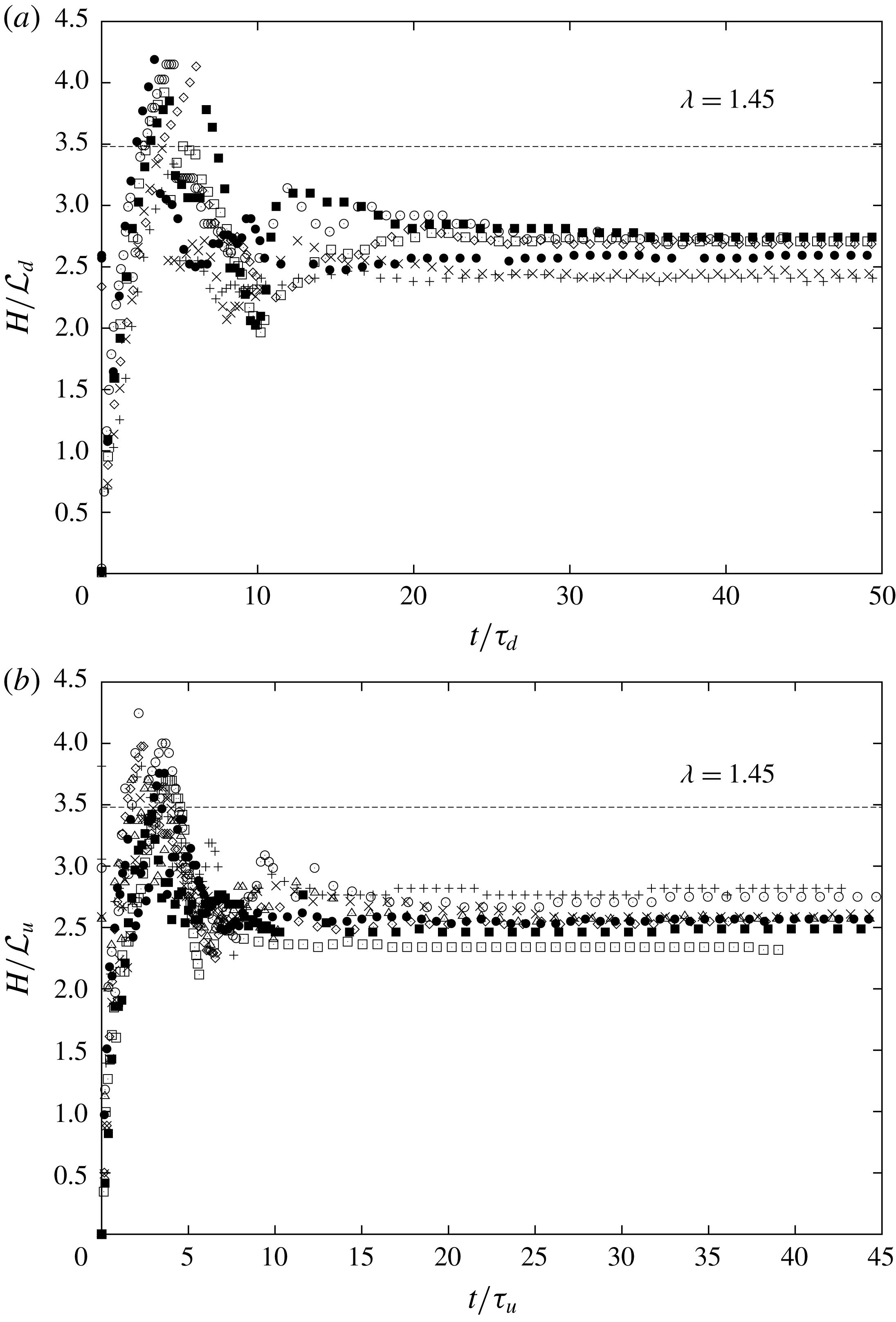
. Based on these length and time scales and on the criteria defined in appendix B, it is therefore possible to plot the time history of the fountain penetration
 $H(t)$
in non-dimensional form, from the initial rise height to the steady state. Figure 5(a) depicts the time history for the downward non-Boussinesq releases. First, during the initial phase, the fountain rises up to reach its maximum height
 $H_{i}/{\mathcal{L}}_{d}\sim 3.6$
at
 $t/\unicode[STIX]{x1D70F}\sim 5$
. Then, due to the presence of the downflow, the fountain collapses and reaches a minimum height at
 $t/\unicode[STIX]{x1D70F}\sim 10$
, corresponding to
 $H_{min}/{\mathcal{L}}_{d}\sim 2$
. From
 $t/\unicode[STIX]{x1D70F}\sim 20$
, the fountain reaches a steady state height,
 $H_{ss}/{\mathcal{L}}_{d}\sim 2.5$
. We particularly note that the ratio of the initial height to the steady state height, noted
 $\unicode[STIX]{x1D706}=H_{i}/H_{ss}$
, is close to
 $1.45$
, as is the case for Boussinesq fountains. Similarly to the ratio
 $\unicode[STIX]{x1D706}$
, it is also possible to define the ratio
 $\unicode[STIX]{x1D6FE}=H_{min}/H_{ss}$
between the minimum height
 $H_{min}$
reached for the first collapse of the fountain and the steady state height
 $H_{ss}$
. We note that
 $\unicode[STIX]{x1D6FE}\sim 0.8$
. Figure 5(b) shows the time history for the upward non-Boussinesq releases. We underline that the behaviour of the penetration height obeys a similar trend to that of the downward release. In particular, we note that the geometric ratios
 $H_{i}/{\mathcal{L}}_{u}\sim 3.6$
,
 $H_{min}/{\mathcal{L}}_{u}\sim 2$
and
 $H_{ss}/{\mathcal{L}}_{u}\sim 2.5$
are similar to the downward release. Nevertheless, we observe that the instants to reach the maximum initial height
 $H_{i}$
, the minimum height
 $H_{min}$
and the steady state height
 $H_{ss}$
are slightly advanced. Note that figures 5(a) and (b) show scatter of the order of
 $\pm 20\,\%$
in the transient phase. Such a scatter is not surprising in turbulent fountain experiments especially for moderate Froude number
 $Fr$
(from 5 to 12), as discussed in Burridge & Hunt (Reference Burridge and Hunt2012). Indeed, by extending their conclusions to the case of turbulent non-Boussinesq fountains, that is by replacing
 $Fr$
by
 $Fr_{NB_{d}}$
or
 $Fr_{NB_{u}}$
, it appears that this scatter is natural because the present study mainly explored the range of moderate Froude numbers.
Penetration height (a)
 $H/{\mathcal{L}}_{d}$
as a function of time
 $t/\unicode[STIX]{x1D70F}_{d}$
for downward releases. Data symbols indicate:
 $+$
,
 $\unicode[STIX]{x1D70C}_{i}/\unicode[STIX]{x1D70C}_{0}=0.05,Fr=23.72$
;
 $\times$
,
 $\unicode[STIX]{x1D70C}_{i}/\unicode[STIX]{x1D70C}_{0}=0.08,Fr=19.78$
; ♢,
 $\unicode[STIX]{x1D70C}_{i}/\unicode[STIX]{x1D70C}_{0}=0.15,Fr=11.07$
; ▫,
 $\unicode[STIX]{x1D70C}_{i}/\unicode[STIX]{x1D70C}_{0}=0.20,Fr=11.07$
; ▪,
 $\unicode[STIX]{x1D70C}_{i}/\unicode[STIX]{x1D70C}_{0}=0.25,Fr=11.19$
; ○,
 $\unicode[STIX]{x1D70C}_{i}/\unicode[STIX]{x1D70C}_{0}=0.35,Fr=9.45$
; ●,
 $\unicode[STIX]{x1D70C}_{i}/\unicode[STIX]{x1D70C}_{0}=0.40,Fr=11.07$
. (b)
 $H/{\mathcal{L}}_{u}$
as a function of time
 $t/\unicode[STIX]{x1D70F}_{u}$
for upward releases. Data symbols indicate:
 $+$
,
 $\unicode[STIX]{x1D70C}_{i}/\unicode[STIX]{x1D70C}_{0}=2.0,Fr=7.91$
;
 $\times$
,
 $\unicode[STIX]{x1D70C}_{i}/\unicode[STIX]{x1D70C}_{0}=3.0,Fr=5.54$
; ♢,
 $\unicode[STIX]{x1D70C}_{i}/\unicode[STIX]{x1D70C}_{0}=4.0,Fr=5.54$
; ▫,
 $\unicode[STIX]{x1D70C}_{i}/\unicode[STIX]{x1D70C}_{0}=4.0,Fr=7.91$
; ▪,
 $\unicode[STIX]{x1D70C}_{i}/\unicode[STIX]{x1D70C}_{0}=5.0,Fr=3.96$
; ○,
 $\unicode[STIX]{x1D70C}_{i}/\unicode[STIX]{x1D70C}_{0}=6.0,Fr=3.16$
; ▪,
 $\unicode[STIX]{x1D70C}_{i}/\unicode[STIX]{x1D70C}_{0}=6.0,Fr=5.54$
; ▵,
 $\unicode[STIX]{x1D70C}_{i}/\unicode[STIX]{x1D70C}_{0}=8.0,Fr=2.37$
. Note that the points on the steady state correspond to the averaged value of
 $H_{ss}$
whereas the points on the transient phase correspond to instantaneous measurements.
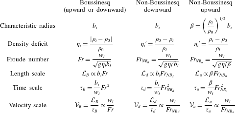
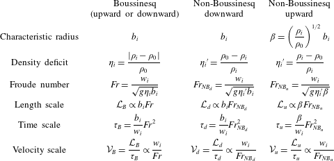
Finally, for the three cases of release, Boussinesq (upward or downward), downward and upward non-Boussinesq, we summarize in table 1 the length and the time scalings for the fountain heights. In this table also appear for each release the input data, i.e. the characteristic source radius, the source density deficit and the source Froude number on which the length, time and velocity scale are built.
Expression for the three cases, Boussinesq (upward or downward), downward non-Boussinesq and upward non-Boussinesq, of the source characteristic radius, the source density deficit, the source Froude number, the length scale, the time scale and the velocity scale.
5 Conclusion
Turbulent forced fountains issuing from a source release of density
 $\unicode[STIX]{x1D70C}_{i}$
into a uniform ambient of density
 $\unicode[STIX]{x1D70C}_{0}$
have been studied numerically by large-eddy simulations. Density ratios
 $\unicode[STIX]{x1D70C}_{i}/\unicode[STIX]{x1D70C}_{0}$
far from the unity (non-Boussinesq conditions) were considered as well as downward and upward directions of injection. It is shown that, depending on the direction of injection, the penetration height of the fountain does not follow the same scaling as it is the case for Boussinesq fountains. For the downward case, a characteristic length scale is
 ${\mathcal{L}}_{d}=b_{i}Fr_{NB_{d}}$
where
 $Fr_{NB_{d}}=w_{i}/\sqrt{g{\unicode[STIX]{x1D702}_{i}}^{\prime }b_{i}}$
is the downward non-Boussinesq Froude number and the density deficit
 ${\unicode[STIX]{x1D702}_{i}}^{\prime }$
is based on the source density, i.e.
 ${\unicode[STIX]{x1D702}_{i}}^{\prime }=(\unicode[STIX]{x1D70C}_{0}-\unicode[STIX]{x1D70C}_{i})/\unicode[STIX]{x1D70C}_{i}$
. For the upward case,
 ${\mathcal{L}}_{u}=\unicode[STIX]{x1D6FD}Fr_{NB_{u}}$
where
 $\unicode[STIX]{x1D6FD}=(\unicode[STIX]{x1D70C}_{i}/\unicode[STIX]{x1D70C}_{0})^{1/2}b_{i}$
is a modified radius and
 $Fr_{NB_{u}}=w_{i}/\sqrt{g{\unicode[STIX]{x1D702}_{i}}^{\prime }\unicode[STIX]{x1D6FD}}$
is the upward non-Boussinesq Froude number. Based on this scaling, a simple behaviour is found for the steady height, i.e.
 $H_{ss}\simeq 2.4{\mathcal{L}}$
for both the upward and downward non-Boussinesq case and also encompasses the Boussinesq case.
Another remarkable feature is the universal trend of the penetration height from the initial rise to the steady state. In particular, the ratio between the maximum initial height
 $H_{i}$
and the steady state height
 $H_{ss}$
, noted
 $\unicode[STIX]{x1D706}=H_{i}/H_{ss}$
, is found to be close to 1.45. Finally, it is surprising to note that the non-Boussinesq plume theory (validated by Ricou & Spalding (Reference Ricou and Spalding1961) for plumes with
 $\unicode[STIX]{x1D70C}_{i}/\unicode[STIX]{x1D70C}_{0}\ll 1$
) allows us to recover the relevant scaling for upward non-Boussinesq fountains, i.e. for
 $\unicode[STIX]{x1D70C}_{i}/\unicode[STIX]{x1D70C}_{0}\gg 1$
. This observation suggests that a similar analogy may exist between a downward heavy non-Boussinesq plume and a downward light non-Boussinesq fountain. This also suggests that, similarly to downward and upward non-Boussinesq fountains, non-Boussinesq downward and upward plumes may also present an asymmetric behaviour.
Appendix A. Computational domain dimensions
The choice of the dimensions of the computational domain is based on the expected geometrical characteristics of the simulated fountain, namely its maximum height and its downflow radius. These geometrical characteristics are hereafter exposed as a function of the length scale
 ${\mathcal{L}}$
discussed in § 4.1 (
 ${\mathcal{L}}={\mathcal{L}}_{u}$
and
 ${\mathcal{L}}={\mathcal{L}}_{d}$
for respectively upward and downward turbulent non-Boussinesq fountains). For the height of the domain,
 $L$
, given that the maximum initial height of the fountain is
 $H_{i}/{\mathcal{L}}\simeq 3.5$
, we have chosen
 $L\simeq 1.33H_{i}$
, i.e.
 $L/{\mathcal{L}}\simeq 4.7$
. We recall that in Williamson et al. (Reference Williamson, Armfield and Lin2011), the vertical extent is given by
 $L/{\mathcal{L}}\simeq 4.5$
. The distance
 $L_{1z}$
specified in the text corresponds to the initial height
 $H_{i}$
of the fountain, i.e.
 $L_{1z}/{\mathcal{L}}\simeq 3.5$
. For the lateral extent
 $l$
, we choose values close to that of Williamson et al. (Reference Williamson, Armfield and Lin2011) by considering
 $(l/2)\simeq 1.75r_{da}$
, where
 $r_{da}$
is the radius of the fountain downflow. This radius corresponds to the frontier between the fountain and the ambient fluid (see Williamson et al.
Reference Williamson, Armfield and Lin2011). In our numerical simulations, it was shown that the fountain radius
 $r_{da}$
was on average of the order
 $2{\mathcal{L}}$
. Consequently, we have chosen
 $l/{\mathcal{L}}\simeq 7$
. Concerning the subregion
 $\unicode[STIX]{x1D6FA}_{1}$
, it covers the range
 $[-0.2{\mathcal{L}};0.2{\mathcal{L}}]$
.
Appendix B. Fountain height determination
In this appendix, the criterion for the determination of the fountain height is exposed. First, we stress the fact that the criterion of the null vertical velocity at the top of the fountain,
 $\widetilde{w}=0$
, which has been used for the determination of the steady height
 $H_{ss}$
cannot be used for the transient phase. Actually, during this phase, not only the top of the fountain constantly moves but also the ambient surrounding fluid which is pushed by the top of the fountain. As a consequence, a criterion on the density has to be found. For turbulent Boussinesq fountains, Williamson et al. (Reference Williamson, Armfield and Lin2011) studied the time evolution of the fountain height from the initial rise to the steady state height. They introduced the scalar criterion
 $$\begin{eqnarray}\unicode[STIX]{x1D719}=\frac{\unicode[STIX]{x1D702}_{m}}{\unicode[STIX]{x1D702}_{i}}=\frac{\displaystyle \frac{\overline{\unicode[STIX]{x1D70C}}-\unicode[STIX]{x1D70C}_{0}}{\unicode[STIX]{x1D70C}_{0}}}{\displaystyle \frac{\unicode[STIX]{x1D70C}_{i}-\unicode[STIX]{x1D70C}_{0}}{\unicode[STIX]{x1D70C}_{0}}}\end{eqnarray}$$
to identify the top of the fountain for
 $r=0$
. In practice, they considered a fixed value of the criterion, namely
 $\unicode[STIX]{x1D719}=0.1$
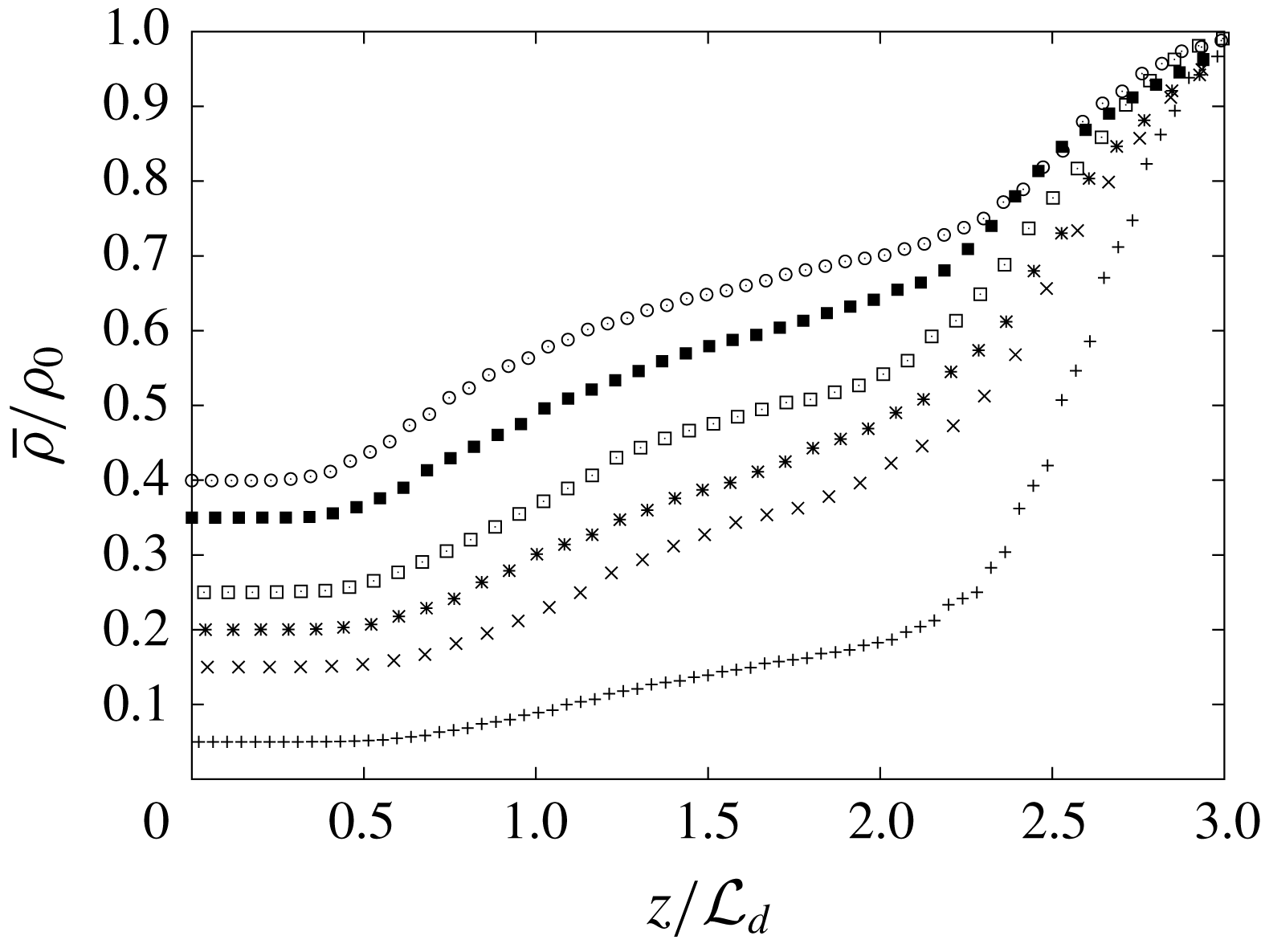
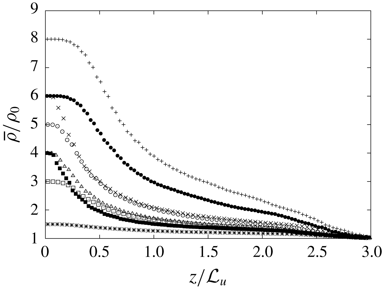
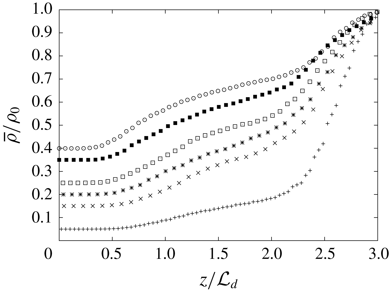
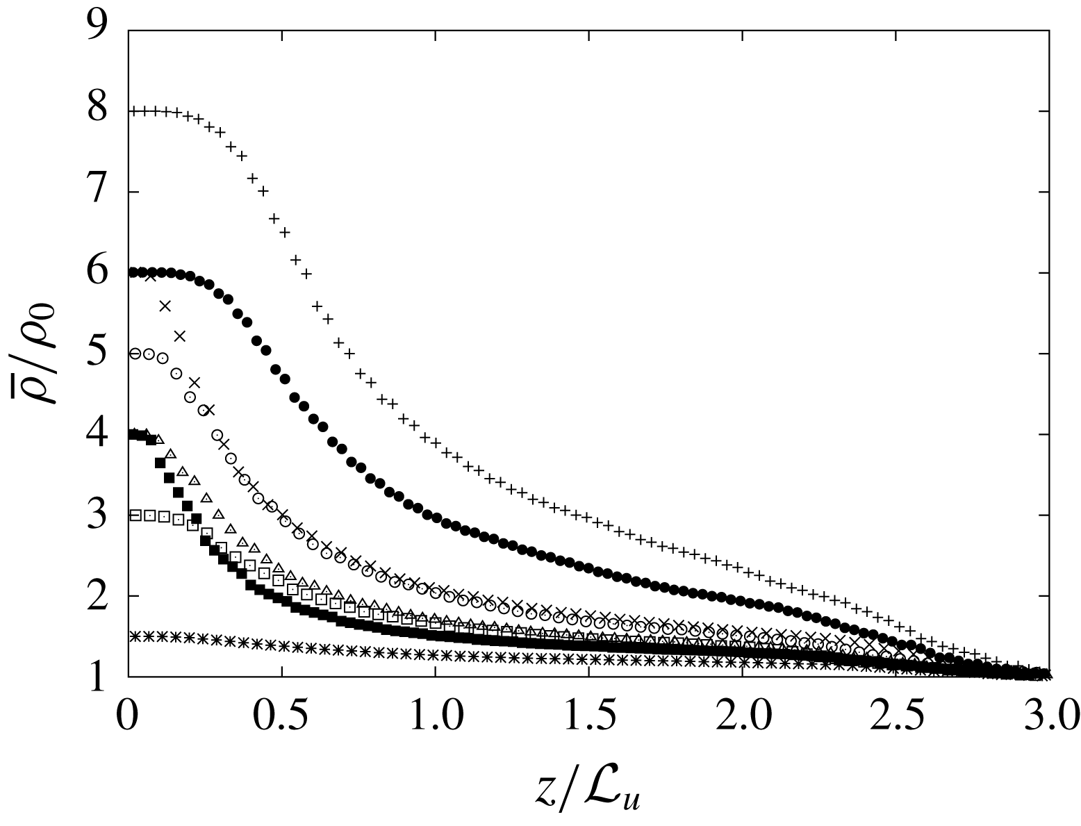
, corresponding to the vertical location where the relative density difference is divided by a factor of 10. In this case, the density at the top of the fountain is found to be extremely close to the density of the ambient. In the present study of turbulent non-Boussinesq fountains, a similar criterion based on the density is proposed. When we look at the vertical density profiles for the simulated upward and downward forced turbulent fountains (see figures 6 and 7) at steady state, two main remarks can be formulated. First, we note that the vertical evolution of the densities differ following the direction of injection. Second, the relative density difference with the ambient of the fountain top is observed to be always greater than
 $15\%$
, indicating that the fountain is still non-Boussinesq at the height
 $H_{ss}$
. Based on these remarks, defining a unique value of a single criterion valid for the two directions is not possible. Thus, we choose to define two different criteria depending on the direction of injection. For the downward injection, we define the penetration height
 $H(t)$
as the first vertical location where the quantity
 $$\begin{eqnarray}\unicode[STIX]{x1D6FE}=\frac{\unicode[STIX]{x1D701}_{m}}{\unicode[STIX]{x1D702}_{i}^{\prime }}=\frac{\displaystyle \frac{\unicode[STIX]{x1D70C}_{0}-\overline{\unicode[STIX]{x1D70C}}}{\overline{\unicode[STIX]{x1D70C}}}}{\displaystyle \frac{\unicode[STIX]{x1D70C}_{0}-\unicode[STIX]{x1D70C}_{i}}{\unicode[STIX]{x1D70C}_{i}}},\end{eqnarray}$$
is inferior to a threshold value of
 $\unicode[STIX]{x1D6FE}=0.075$
. For the upward case, we define the penetration height
 $H(t)$
as the first vertical location where the quantity
 $$\begin{eqnarray}\unicode[STIX]{x1D713}=\frac{\unicode[STIX]{x1D701}_{m}}{\unicode[STIX]{x1D702}_{i}}=\frac{\displaystyle \frac{\overline{\unicode[STIX]{x1D70C}}-\unicode[STIX]{x1D70C}_{0}}{\overline{\unicode[STIX]{x1D70C}}}}{\displaystyle \frac{\unicode[STIX]{x1D70C}_{i}-\unicode[STIX]{x1D70C}_{0}}{\unicode[STIX]{x1D70C}_{0}}},\end{eqnarray}$$
is inferior to a threshold value of
 $0.075$
.
Vertical evolution (for
 $r=0$
) of the density ratio
 $\overline{\unicode[STIX]{x1D70C}}/\unicode[STIX]{x1D70C}_{0}$
for downward releases at steady state.
Vertical evolution (for
 $r=0$
) of the density ratio
 $\overline{\unicode[STIX]{x1D70C}}/\unicode[STIX]{x1D70C}_{0}$
for upward releases at steady state.
Appendix C. Source parameters of fountain simulations and the corresponding steady state height
 $H_{ss}$

Source parameters of fountain simulations (downward injection for
 $\unicode[STIX]{x1D70C}_{i}/\unicode[STIX]{x1D70C}_{0}<1$
and upward injection for
 $\unicode[STIX]{x1D70C}_{i}/\unicode[STIX]{x1D70C}_{0}>1$
) and the corresponding steady state height
 $H_{ss}$
. The Reynolds number is defined as
 $Re=2w_{m}b_{i}/\unicode[STIX]{x1D708}$
where
 $\unicode[STIX]{x1D708}$
is the kinematic viscosity. Note that the mean velocity
 $w_{i}$
is based on a turbulent pipe flow profile which leads us to
 $w_{i}=72/91w_{m}$
where
 $w_{m}$
is the maximum velocity at the radial coordinate
 $r=0$
. The gases, air, helium, carbon dioxide (
 $\text{CO}_{2}$
) and sulphur hexafluoride (
 $\text{SF}_{6}$
) have been taken at
 $1~\text{atm}$
and
 $20~^{\circ }\text{C}$
.