


1. Introduction
Ideally we would want to model stars from their center to their outermost regions using one unified model. However as different physical processes become dominant in the atmosphere of stars and in their center this unification is in practice numerically unfeasible. There is thus a decoupling in the way we model stars. On one hand we use stellar evolution codes, which compute the evolution of the internal structure of stars and produce evolutionary tracks. On the other hand we use stellar atmosphere codes, which perform detailed radiative transfer simulations in order to determine the structure of the atmosphere of stars and to compute synthetic spectra.
Stellar evolution codes need boundary conditions at their surface in order to close the set of stellar structure and evolution (SSE) equations, which form a coupled differential equation system. These boundary conditions must come from a model atmosphere. However it is too time-consuming to compute a realistic model atmosphere at each time-step of an evolution model. Thus the Eddington gray approximation, a very simplified model atmosphere, is generally used to provide the boundary conditions needed for the evolution computations to be performed. The Eddington gray approximation is analytic and therefore easy to implement.
There have been attempts to include realistic model atmospheres in massive star evolution computations in the past. This can be done for instance in post-processing. The idea is to first compute an Eddington gray evolution model. Then for several points of the resulting evolutionary track a model atmosphere is computed using as an input the stellar parameters coming from the evolutionary track. Then a new value of the photospheric radius is extracted from this model atmosphere and is used to recompute the effective temperature. The new effective temperature is then substituted into the Eddington gray one. The main drawback from this method is that there is no feedback from the model atmosphere onto the evolution model through the boundary conditions. Post-processing was notably used by Groh et al. (Reference Groh, Meynet, Ekström and Georgy2014) on the evolutionary track of a  $60 M_{\odot}$ star at solar metallicity. This study showed that the recomputed effective temperatures are close to the Eddington gray ones for the main sequence evolution. However for the later stages of the evolution the effective temperatures derived from realistic model atmospheres are significantly lower than the Eddington gray ones.
Another method is direct code-coupling, which was done by Schaerer et al. (Reference Schaerer, de Koter, Schmutz and Maeder1996). The concept is to directly include a radiative transfer simulation inside an evolution code. At each iteration and for each time-step a model atmosphere is computed using the stellar parameters from the evolution model as an input. This model atmosphere is then used to compute the radius and the effective temperature of the star, and to provide boundary conditions to the evolution model. There is an iterative process so that both the internal and atmospheric structure converge. The main drawback of this method is that for it to be feasible in a acceptable computing time the model atmosphere needs to be very simplified compared to what is done in state-of-the-art atmosphere codes. In their study Schaerer et al. (Reference Schaerer, de Koter, Schmutz and Maeder1996) used this method to compute the main sequence evolution of a  $60 M_{\odot}$ star at solar metallicity, finding almost no differences compared to an Eddington gray track.
However including realistic model atmospheres in massive stars evolution computations has never been done in a self-consistent way. This is the purpose of this study.
2. Methods
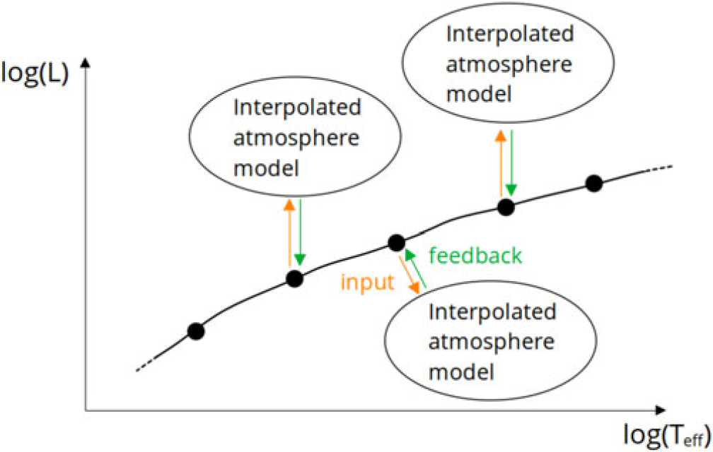
We rely on the method presented by Schaerer et al. (Reference Schaerer, de Koter, Schmutz and Maeder1996) to include realistic model atmospheres. A schematic representation of the method we developed is shown in Figure 1. This method can be summarized as follows. We first compute an Eddington gray evolution model. We then compute a grid of realistic model atmospheres which encompass the Eddington gray evolutionary track. We then compute an evolution model taking into account realistic atmospheres. At each iteration of each time-step we interpolate a model atmosphere within our grid. This model is used to compute the effective temperature of the stellar model and to provide the boundary conditions on temperature and density which are necessary for the evolution model. This method is applied routinely in low-mass stars evolution model (see for example Chabrier and Baraffe Reference Chabrier and Baraffe1997; Chen et al. Reference Chen, Girardi and Bressan2014; Baraffe et al. Reference Baraffe, Homeier, Allard and Chabrier2015; Mosumgaard et al. Reference Mosumgaard, Ball and Silva Aguirre2018; Amard et al. Reference Amard, Palacios and Charbonnel2019). This method has a very limited computational cost compared to the “on-the-fly” coupling to a radiative transfer code, and makes possible the inclusion of realistic model atmospheres in massive stars evolution computations.
Schematic representation of our self-consistent method to include realistic atmospheres in massive stars evolution computation.

We use the stellar evolution code STAREVOL (Amard et al. Reference Amard, Palacios and Charbonnel2019), which solves the SSE equations using the Henyey scheme (Henyey et al. Reference Henyey, Forbes and Gould1964). To compute our model atmospheres we use the atmosphere code CMFGEN (Hillier and Miller Reference Hillier and Miller1998). CMFGEN is a state of the art non-Local Thermodynamic Equilibrium atmosphere code which takes into account sphericity, wind extension and line-blanketing.
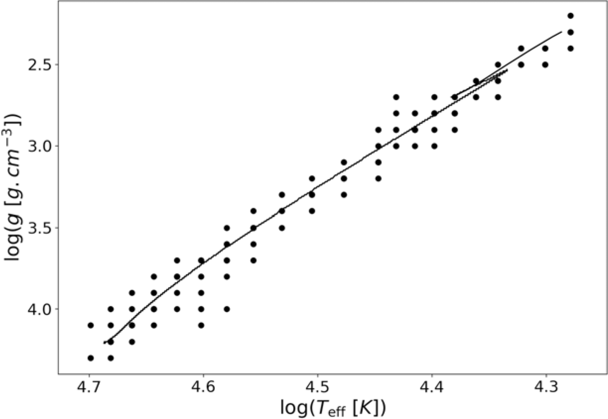
We apply our method to a  $60 M_{\odot}$ single stellar model at solar metallicity and without rotation. This choice was made in order to compare our results with those of the previous studies of Groh et al. (Reference Groh, Meynet, Ekström and Georgy2014) and Schaerer et al. (Reference Schaerer, de Koter, Schmutz and Maeder1996). We represent our model atmosphere grid in the Kiel diagram along with an Eddington gray model for the main sequence evolution in Figure 2. As we can see the grid encompasses the evolutionary track.
Representation of our grid in the Kiel diagram for the main sequence evolution along with an Eddington gray evolutionary track.

The interpolation is performed in the parameter space ( $T(\tau_\mathrm{match}), \log(g), \log(\dot{M})$), where :
•
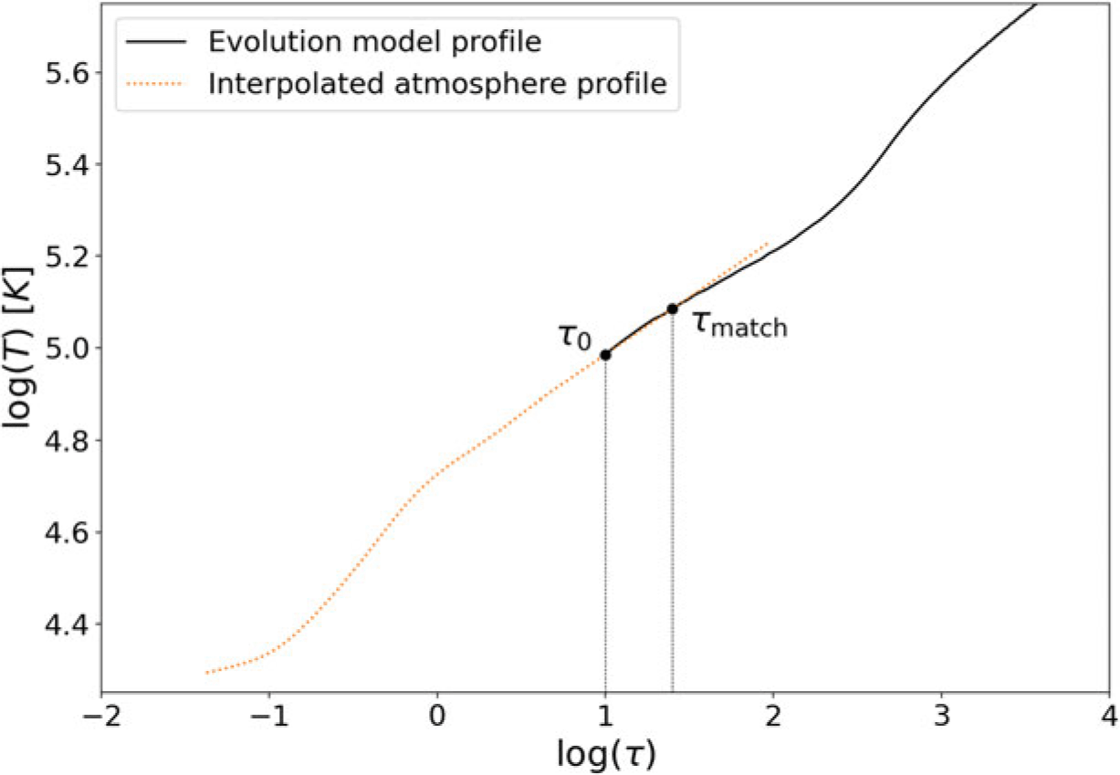
 $T(\tau_\mathrm{match})$ is the temperature of the evolution model at an optical depth $\tau_\mathrm{match}$ which is a fixed parameter chosen to be located where the diffusion approximation is valid. This choice is based on the fact that in the diffusion approximation the model atmosphere’s temperature structure is supposed to be the same as the evolution model’s. For the models we present here we used $\tau_\mathrm{match} = 25$.
-
•
$g = GM_*/R_*^2$ is the gravity at the photosphere. -
•
$\dot{M}$ is the mass-loss rate, which is computed in the evolution model.


We interpolate a temperature, a density and a radius profile. We use the temperature and density profiles to apply boundary conditions at the numerical surface of the evolution model. This numerical surface is located at a fixed optical depth  $\tau_0 = 10$, where again the diffusion approximation holds. For optical depths
 $\tau \lt \tau_0$ we patch the interpolated atmosphere structure. We assume the luminosity
 $L_*$, the mass
 $M_*$ and the chemical composition to be constant in this region (their values being taken from the evolution model at the numerical surface). We show in Figure 3 the temperature profile of the evolution model at a given time-step along with the interpolated atmosphere profile. We also highlight the positions of
 $\tau_0$ and
 $\tau_\mathrm{match}$.
Evolution (in black) and model atmospheres (in orange) temperature profiles a functions of the Rosseland optical depth.

The photospheric radius  $R_*$ is read from the radius atmosphere profile at an optical depth
 $\tau = 2/3$. This choice to define the photosphere at
 $\tau = 2/3$ is made in order to assure consistency with the Eddington gray evolution models. We then compute the effective temperature
 $T_\mathrm{eff} = L_* / (4 \pi \sigma R_*^2)$ and the gravity at the photosphere g.
3. Results
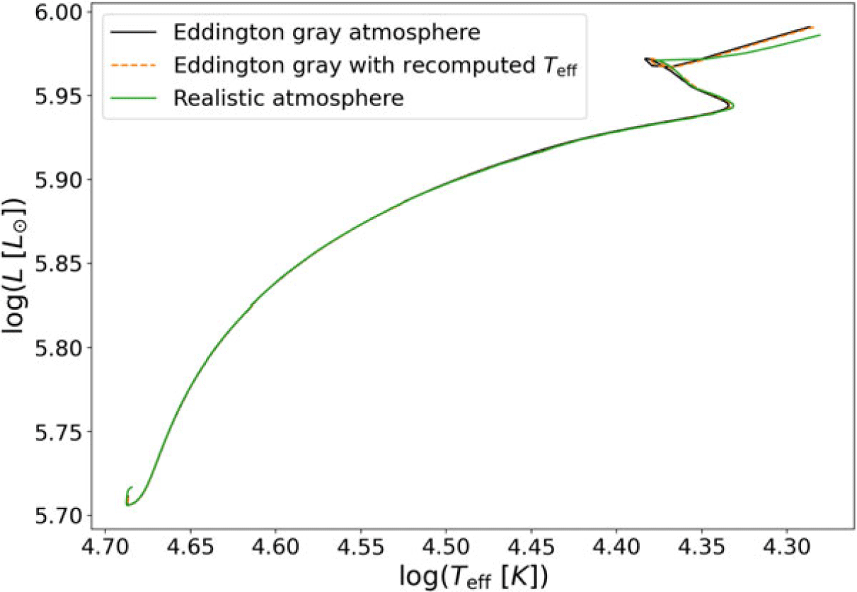
We plot the results obtained with our self-consistent method on the main sequence in Figure 4 along with an Eddington gray model. We find that the inclusion of realistic atmospheres does not modify the main sequence evolutionary track for a  $60 M_{\odot}$ star at solar metallicity. This result is consistent with the previous findings of Groh et al. (Reference Groh, Meynet, Ekström and Georgy2014) and Schaerer et al. (Reference Schaerer, de Koter, Schmutz and Maeder1996). We also verified this finding using another method based on the Hopf function (Hubeny Mihalas Reference Hubeny and Mihalas2014).
Hertzsprung-Russell diagram showing an evolutionary track including realistic atmospheres with our self-consistent method (in green) compared with one including realistic atmospheres in post-processing (in orange) and an Eddington gray computation (in black) for the main sequence evolution.

We performed a post-processing test similar to the one of Groh et al. (Reference Groh, Meynet, Ekström and Georgy2014) on the main-sequence Eddington gray model. For each time-step of the evolution we interpolated model atmospheres using the method described above. We then used these models to recompute the effective temperature of the evolution model. As this is post-processing, the recomputed effective temperature is not used during the evolution computation, and we use the Eddington gray boundary conditions to close the SSE equations system. Using this method we find almost no differences between the Eddington gray effective temperature and the one recomputed using realistic model atmospheres. This confirms that the Eddington gray approximation is valid for the main sequence evolution of a  $60 M_{\odot}$ star at solar metallicity.
4. Conclusion
We implemented a method to perform massive stars evolution computations including realistic model atmospheres and we tested it on a  $60 M_{\odot}$ stellar model at solar metallicity. We confirm that the Eddington gray approximation is valid on the main sequence evolution.