1. Introduction
The lymphatic system is responsible for transportation of interstitial fluid, lipids and immune cells to maintain homeostasis throughout the body. Interstitial fluid and macromolecules collected and circulated by the lymphatic system join the blood circulatory system to maintain tissue fluid balance and waste management. Fatty acid is collected in the gut from food, packaged into chylomicrons and transported via the lymphatic system as the primary route of lipid trafficking to the peripheral tissues, and transported immune cells and antigens provide a proper immune response (Swartz Reference Swartz2001; Dixon Reference Dixon2010). Nearly all tissues in the body critically rely on the lymphatic system for proper operation, yet this is achieved without a centralized pump and under an adverse pressure gradient. Instead, circulation is achieved by a combination of nearby tissues’ skeletal muscular movement (extrinsic pump) (Webb & Starzl Reference Webb and Starzl1953; Reddy, Palmieri & Cochran Reference Reddy, Palmieri and Cochran1981; Skalak, Schmid-Schönbein & Zweifach Reference Skalak, Schmid-Schönbein and Zweifach1984; McGeown, McHale & Thornbury Reference McGeown, McHale and Thornbury1988; Ikomi & Schmid-Schonbein Reference Ikomi and Schmid-Schonbein1996) and a series of contracting vessels and valves throughout the collecting lymphatics, known as the intrinsic lymphatic pump (Quick et al. Reference Quick, Venugopal, Gashev, Zawieja and Stewart2007; Zawieja Reference Zawieja2009; Davis et al. Reference Davis, Rahbar, Gashev, Zawieja and Moore2011). The intrinsic lymphatic pump is composed of chains of contractile units called lymphangions, defined as a region of the lymphatic vessel separated by two lymphatic valves. For an efficient transport of lymphatic fluids in the desired direction, lymphatic valves play a critical role by reducing backflow and maximizing the net flow, often against a gravitational load.
Dysfunction of the lymphatic valves or smooth muscles that drive contractile motion of the lymphatic vessels can lead to debilitating conditions of lymphedema, for which there is currently no cure (Mortimer & Rockson Reference Mortimer and Rockson2014). Palliative treatment options, such as compression garments, do exist, but these methods only seek to relieve the symptoms of disease without addressing the underlying cause. In some cases, like genetic primary lymphedema, lymphatic valve defects have been identified as a major source of dysfunction (Eisenhoffer et al. Reference Eisenhoffer, Kagal, Klein and Johnston1995; Petrova et al. Reference Petrova, Karpanen, Norrmén, Mellor, Tamakoshi, Finegold, Ferrell, Kerjaschki, Mortimer and Ylä-Herttuala2004; Davis et al. Reference Davis, Scallan, Wolpers, Muthuchamy, Gashev and Zawieja2012; Brouillard, Boon & Vikkula Reference Brouillard, Boon and Vikkula2014; Sabine et al. Reference Sabine, Bovay, Demir, Kimura, Jaquet, Agalarov, Zangger, Scallan, Graber and Gulpinar2015; Lapinski et al. Reference Lapinski, Lubeck, Chen, Doosti, Zawieja, Davis and King2017). While many of these studies have identified the molecular mechanism responsible for the morphologic valve defect, the structure–function relationship of lymphatic valves and the exact consequence of subtle valve defects on the pump performance of the lymphatic network are less understood. In addition, the role that factors like the heterogeneity of lymphatic valves play has been studied but is still largely unknown.
To address this limited understanding, computational studies have been providing valuable insights in creating a detailed picture of lymphatic operation and have indicated that lymphatic valve's properties affect the pumping performance of the lymphatic system (Davis et al. Reference Davis, Rahbar, Gashev, Zawieja and Moore2011; Bertram, Macaskill & Moore Reference Bertram, Macaskill and Moore2014b; Wilson et al. Reference Wilson, van Loon, Wang, Zawieja and Moore2015). These computational studies range from lumped-parameter models that solve differential equations combined with experimental data (Reddy, Krouskop & Newell Reference Reddy, Krouskop and Newell1977; Bertram, Macaskill & Moore Reference Bertram, Macaskill and Moore2011; Jamalian et al. Reference Jamalian, Bertram, Richardson and Moore2013, Reference Jamalian, Davis, Zawieja and Moore2016; Bertram et al. Reference Bertram, Macaskill, Davis and Moore2014a,Reference Bertram, Macaskill and Mooreb, Reference Bertram, Macaskill, Davis and Moore2016; Baish et al. Reference Baish, Kunert, Padera and Munn2016; Razavi et al. Reference Razavi, Nelson, Nepiyushchikh, Gleason and Dixon2017) to multi-dimensional studies of fluid and solid components involved in lymph flow (MacDonald et al. Reference MacDonald, Arkill, Tabor, McHale and Winlove2008; Rahbar & Moore Reference Rahbar and Moore2011; Kunert et al. Reference Kunert, Baish, Liao, Padera and Munn2015; Wilson et al. Reference Wilson, van Loon, Wang, Zawieja and Moore2015; Bertram Reference Bertram2020). However, many of these studies employ assumptions or simplifications, particularly in regard to valve behaviour, providing only a limited understanding of the role of the lymphatic valve in lymphatic transport performance and efficiency. For example, the lumped-parameter model or zeroth-dimensional study utilizes a valve resistance curve that is an empirical fit of lymphatic valve behaviour based on a single set of experimental data points (Bertram et al. Reference Bertram, Macaskill and Moore2011; Bertram, Macaskill & Moore Reference Bertram, Macaskill and Moore2014b). Most of these studies can effectively simulate chains of lymphangions, thus revealing large-scale behaviours of lymphangion networks. However, because of the rarity of measured lymphatic valve properties (Lauweryns & Boussauw Reference Lauweryns and Boussauw1973; MacDonald et al. Reference MacDonald, Arkill, Tabor, McHale and Winlove2008; Pan, Le Roux & Levy Reference Pan, le Roux and Levy2011; Wilson et al. Reference Wilson, van Loon, Wang, Zawieja and Moore2015), the empirical fit that describes the lymphatic valve's flow response is limited in describing lymphatic performance and efficiency under different valve properties such as valve length and stiffness.
Higher-dimensional models of the lymphatic system can address this limitation by modelling the lymphatic valve based on the more readily available geometric profile of the valve (Wilson et al. Reference Wilson, van Loon, Wang, Zawieja and Moore2015; Bertram Reference Bertram2020), but these models also simplify the physics through assumptions such as a steady flow condition (Wilson et al. Reference Wilson, van Loon, Wang, Zawieja and Moore2015), exclusion of components that require fluid–structure interaction like the lymphatic valves (Rahbar & Moore Reference Rahbar and Moore2011) or using externally applied fluid flow (Bertram Reference Bertram2020). We recently conducted three-dimensional simulations using a fully coupled fluid–structure interaction model to probe the behaviour of compliant lymphatic valves in a fluid flow (Ballard et al. Reference Ballard, Wolf, Nepiyushchikh, Dixon and Alexeev2018). Valves with different geometries and mechanics were placed in a rigid axisymmetric vessel and flow was induced by applying oscillating or unidirectional pressure gradients. It was found that shorter valves have a lower flow resistance, however, when the valves are too short, they are unable to fully occlude the backflow, indicating the existence of an optimal valve length. It was also shown that more flexible valves cause a lower resistance to the flow. Furthermore, under oscillating flow, valve elasticity leads to a delay in valve response that has been reported in experiments (Davis et al. Reference Davis, Rahbar, Gashev, Zawieja and Moore2011).
In this paper, we focus on understanding the pumping behaviour of a peristaltically contracting vessel fitted with compliant valves similar to those found in lymphatic systems (Ohhashi, Azuma & Sakaguchi Reference Ohhashi, Azuma and Sakaguchi1980; Zawieja et al. Reference Zawieja, Davis, Schuster, Hinds and Granger1993). We consider a periodic vessel that undergoes periodic radial contractions leading to a sinusoidal travelling wave (Shapiro, Jaffrin & Weinberg Reference Shapiro, Jaffrin and Weinberg1969; Takabatake, Ayukawa & Mori Reference Takabatake, Ayukawa and Mori1988). We use this model to investigate the effects of elastic valves on pumping performance of peristaltically contracting vessels. Specifically, valve and vessel properties such as vessel contraction wave speed, vessel contraction amplitude and valve elasticity are systematically probed for the peristaltic pumping under a range of applied adverse pressure gradients.
Additional complexity in lymphatic systems emerges due the coupling between the contraction amplitude of the lymphatic vessel and the applied adverse pressure gradient (Davis et al. Reference Davis, Scallan, Wolpers, Muthuchamy, Gashev and Zawieja2012). Experiments show that an increasing adverse pressure gradient results in a decreased contraction amplitude, diminishing the pumping performance of lymphatic vessel. Such behaviour is typically associated with the finite force generation by the lymphatic muscle cells driving contractions. Other physiological features affecting lymphatic pumping include non-uniformity of vessel contraction near the valve (Akl et al. Reference Akl, Coté, Nepiyushchikh, Gashev and Zawieja2011; Davis et al. Reference Davis, Scallan, Wolpers, Muthuchamy, Gashev and Zawieja2012) and lymph flow-sensitive wall contraction via wall shear stress (Gashev, Davis & Zawieja Reference Gashev, Davis and Zawieja2002; Kornuta et al. Reference Kornuta, Nepiyushchikh, Gasheva, Mukherjee, Zawieja and Dixon2015). Here, we examine how the coupling between the adverse pressure gradient and the vessel contraction amplitude affects the pumping performance of peristaltic vessels with elastic valves.
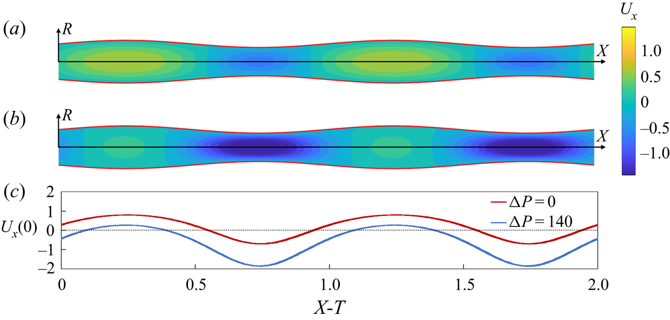
Without valves, peristaltic pumping generates fluid packets with alternating axial velocity that are steady in the moving frame of reference under a constant contraction wave speed, c (figure 1(a) and supplementary movie 1 available at https://doi.org/10.1017/jfm.2021.302). These velocity packets lead to a net transport of the fluid in the direction of wave propagation that we refer to as the positive flow direction. The presence of an adverse pressure gradient can reduce the net fluid pumping by peristaltic oscillations and ultimately can result in a negative flow (figure 1(b) and supplementary movie 1). When the adverse pressure gradient is large enough, sections with positive flow velocity diminish or entirely disappear, even though the general pattern with repeating velocity packets is still maintained (figure 1c). The peristaltic pumping in a vessel without valves provides a baseline that allows us to evaluate the function of valves and to identify their effects on the fluid flow and pumping.
(a) Axial component of flow velocity  ${U_x}$ in a valve-less peristaltic vessel without an imposed pressure gradient yielding a flow rate
 $Q = 0.15$. (b) Axial velocity
 ${U_x}$ in a vessel with an adverse pressure gradient
 $\mathrm{\Delta }P = 140$ yielding a flow rate
 $Q ={-} 0.22$. (c) Centreline axial velocity
 ${U_x}(0)$ in the moving reference frame
 $X - T$. In these simulations, the contraction ratio is
 $\phi = 0.2$, and the peristaltic Reynolds number is
 $Re = 0.2$. Note that
 $X = x/\lambda $,
 $T = t/\tau $,
 $\mathrm{\Delta }P = \Delta {p_\lambda }\; r_0^2\rho /{\mu ^2}$,
 $Q = q/{\rm \pi} r_0^2c$,
 $\phi = a/{r_0}$ and
 $Re = \rho cr_0^2/\mu \lambda $, where
 $\Delta {p_\lambda }$ is the pressure difference across a contraction wavelength, q is the vessel flow rate,
 ${r_0}$ is the mean radius of the vessel, x is the axial coordinate,
 $\rho $ and
 $\mu $ are the fluid density and dynamic viscosity and t is time. Furthermore,
 $\lambda $,
 $\tau $,
 $c$ and a are the wavelength, period, speed and amplitude of vessel contraction. See supplementary movie 1.

The paper is organized as follows. In § 2, we present our computational methodology and the model validation. This section also describes the relevant model parameters. The simulation results are reported and discussed in § 3. Section 3.1 compares peristaltic pumping in vessels with and without valves to identify the effects of the valve on the flow pattern and pumping performance. Section 3.2 investigates the effect of vessel contraction speed on flow behaviour and pumping performance. Section 3.3 studies the effect of an adverse pressure gradient, while § 3.4 examines the effect of valve elasticity on the pumping performance. Section 3.5 considers the effects of coupling between the adverse pressure gradient and the amplitude of the vessel contractions on the fluid pumping. Our conclusions are summarized in § 4.
2. Methodology
To model viscous fluid flow within a peristaltic vessel fitted with elastic valves, a fully coupled three-dimensional fluid–structure interaction solver (FSI) is used. A lattice Boltzmann model (LBM) and a lattice spring model (LSM) are used to simulate the fluid mechanics and solid mechanics, respectively. To capture interactions between fluid and solid, the models are coupled through the boundary conditions as implemented previously (Alexeev, Verberg & Balazs Reference Alexeev, Verberg and Balazs2005; Alexeev & Balazs Reference Alexeev and Balazs2007).
LBM efficiently simulates incompressible viscous flows (Ladd & Verberg Reference Ladd and Verberg2001; Succi Reference Succi2001) and is well suited for studies with complex, moving geometries, such as compliant valves and contracting vessels. LBM simulates the Navier–Stokes equations at mesoscale by integrating the time evolution of the velocity distribution function representing fluid ‘particles’ moving on a fixed lattice  ${f_i}(\boldsymbol{r},t)$, where i,
 $\boldsymbol{r}$ and t are the velocity direction, the lattice position and time, respectively. The distribution function is integrated over discrete time steps via streaming and collision of ‘particles’, where fluid ‘particles’ travel across the lattice in a given speed and direction. In this work, we use the two-relaxation-time (TRT) collision operator and a D3Q19 grid representing a three-dimensional system with 19 discrete velocity directions. Hydrodynamic fields such as density, momentum and stresses are evaluated by taking moments of the distribution function.
Solid components of the system are modelled using LSM (Ostoja-Starzewski Reference Ostoja-Starzewski2002; Buxton et al. Reference Buxton, Verberg, Jasnow and Balazs2005). We represent thin elastic valve material as an infinitely thin elastic plate discretized using a network of masses linked by stretching and bending springs. Solid nodes are arranged in a regular triangular lattice with nearby nodes connected via a linear stretching spring of in-plane stiffness  ${k_s}$. The bending of the plate is modelled through a series of bending springs with bending stiffness
 ${k_b}$, which connect three neighbouring LSM nodes. The related macroscopic properties, such as Young's modulus and bending rigidity, are defined using the in-plane and bending stiffnesses as
 ${e_s} = 2{k_s}/\sqrt 3 $ (Ostoja-Starzewski Reference Ostoja-Starzewski2002) and
 ${d_b} = 3\sqrt 3 {k_b}/4$, respectively (Buxton et al. Reference Buxton, Verberg, Jasnow and Balazs2005).
LBM and LSM interact through a two-way coupling at fluid–solid boundaries with the momentum exchange approach. The momentum due to fluid–solid interaction is transferred to fluid using interpolated bounce-back rule and distributed through corresponding solid nodes via applied forces to ensure momentum conservation (Alexeev et al. Reference Alexeev, Verberg and Balazs2005; Alexeev, Verberg & Balazs Reference Alexeev, Verberg and Balazs2006; Mao & Alexeev Reference Mao and Alexeev2014). This method of coupling has been previously extensively validated with different FSI problems (Masoud, Bingham & Alexeev Reference Masoud, Bingham and Alexeev2012; Mao & Alexeev Reference Mao and Alexeev2014; Yeh & Alexeev Reference Yeh and Alexeev2016; Hanasoge et al. Reference Hanasoge, Ballard, Hesketh and Alexeev2017; Ballard et al. Reference Ballard, Wolf, Nepiyushchikh, Dixon and Alexeev2018).
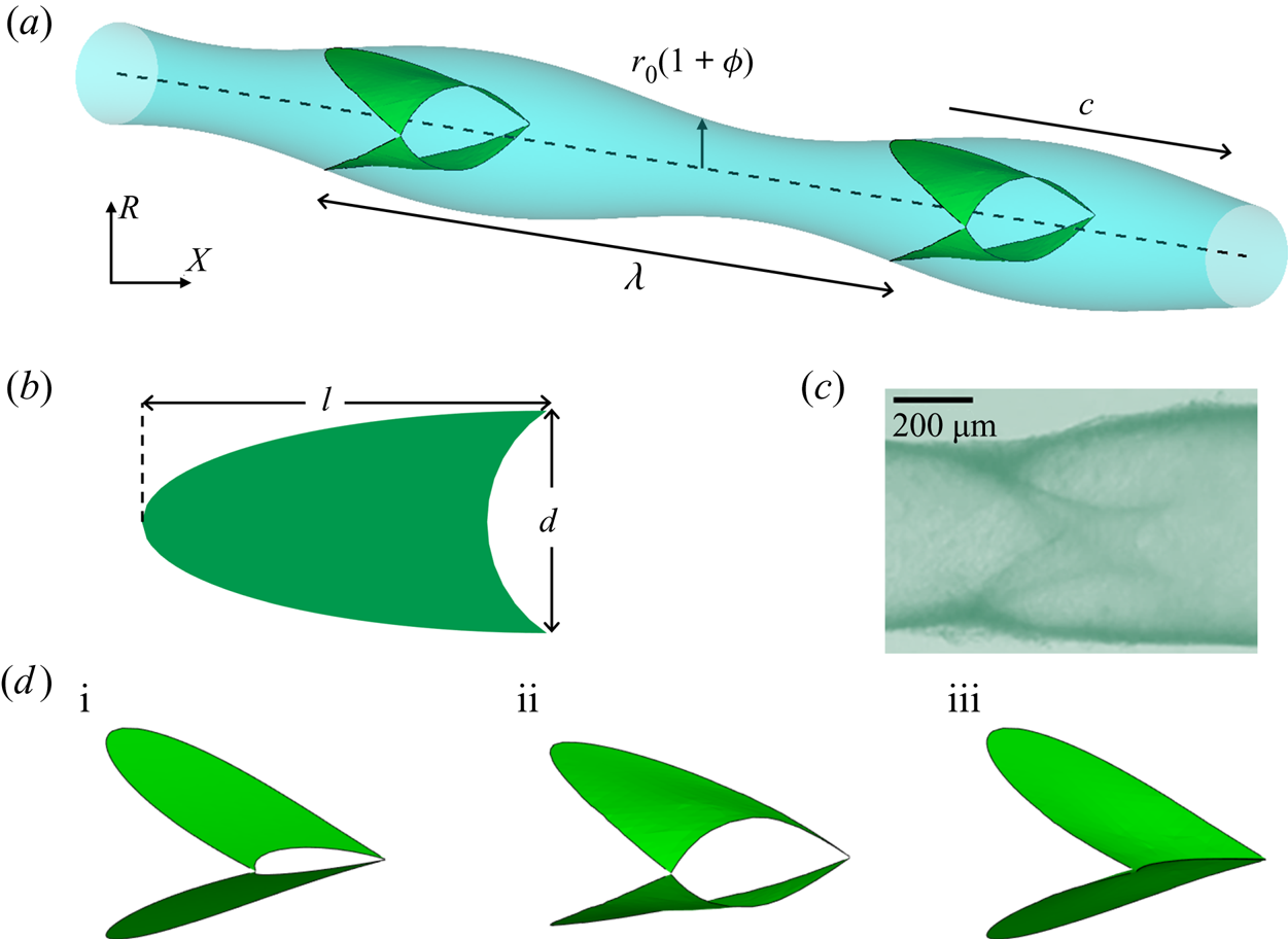
The model is composed of a periodic fluid-filled axisymmetric vessel and two sets of valves, with each valve made up of two compliant leaflets (figure 2 and supplementary movie 2). Each leaflet is created from an intersecting plane between an axisymmetric vessel and a plane that cuts through the vessel at an angle (Ballard et al. Reference Ballard, Wolf, Nepiyushchikh, Dixon and Alexeev2018). Thus, the elastic leaflets are initially flat. The leaflet edge that overlaps with the vessel wall is firmly attached to the wall and follows the wall motion. The free edge of the leaflet has a semi-circular cutout, mimicking the typical geometry observed for lymphatic valves (Watson et al. Reference Watson, Sazonov, Zawieja, Moore and van Loon2017). The valve geometry combined with the axisymmetric vessel mean that it is necessary to use a three-dimensional computational model since lower-dimensional or axisymmetric models are unable to capture the leaflet motion. The leaflet geometry is characterized by the aspect ratio that is defined as the ratio between axial length of the leaflet and mean diameter of the vessel. In this work, we keep the leaflet aspect ratio equal to 1.75 that is in the typical range of experimental values (Ballard et al. Reference Ballard, Wolf, Nepiyushchikh, Dixon and Alexeev2018). The simulation domain has 301 by 44 by 44 LBM nodes in the x, y and z-directions, respectively, while the vessel and valves are composed of 8272 LSM nodes. The initial distance between two neighbouring LSM nodes is approximately twice the distance between neighbouring LBM nodes.
(a) Model of a periodic contracting vessel fitted with two valves. (b) Shape and dimensions of the valve leaflet. The edge on the right side of the leaflet is free, whereas the remaining part of the edge is attached to the vessel wall. The aspect ratio of the valve is defined as  $l/d = 1.75$. (c) Image of a lymphatic vessel segment with a valve. (d) Typical valve profiles during different stages of valve operation. (i) Initial valve configuration, (ii) valve opening and (iii) valve closure. See supplementary movie 2.

The vessel undergoes a prescribed radial motion that leads to a sinusoidal travelling wave propagating along the vessel in the axial x direction. The periodic motion of the vessel wall is given by
 \begin{equation}{r_{vess}}(x,t) = {r_0}\left[ {1 + \phi \sin \left( {\frac{{2{\rm \pi} }}{\lambda }(x - ct)} \right)} \right],\end{equation}
where  ${r_0}$ is the mean radius of the vessel,
 $\phi $ is the normalized contraction amplitude,
 $\lambda $ is the wavelength and
 $c = \lambda /\tau $ is the wave speed with
 $\tau $ being the oscillation period. Note that
 $\phi = a/{r_0}$, where a is the vessel contraction amplitude. We set the wavelength equal to the distance between the centroids of two consecutive valves. The wavelength is kept at a constant value equal to the distance between valves to induce synchronous valve deformation, providing a clearer understanding of the fundamental operation of the valves in contracting vessel. We plan to further explore the effect of contraction wave wavelength in our future works.
Experiments report a wide range of the contraction wavelength,  $\lambda $. Indeed, the wave speed c ranges from zero to
 $10\ \textrm{mm}\ {\textrm{s}^{ - 1}}$ with the frequency between 7 and 21 contractions per minute, yielding a wavelength between 0 and
 $81\ \textrm{mm}$ (MacDonald et al. Reference MacDonald, Arkill, Tabor, McHale and Winlove2008; Akl et al. Reference Akl, Coté, Nepiyushchikh, Gashev and Zawieja2011). Since the vessel diameters typically range from
 $80\ \mathrm{\mu }\textrm{m}$ to
 $2.8\ \textrm{mm}$ and considering that the larger vessels exhibit a longer wavelength, we estimate that the ratio of the wavelength to the vessel radius
 $\lambda /{r_0}$ is in a wide range between 0 and 60. In our simulations, we set
 $\lambda /{r_0} = 15$, which falls well into the experimental range. Furthermore, considering that the inter-valve distance is the same as
 $\lambda $, this puts the valve placement within the experimental range, where the values of this ratio are up to 20 (Pan et al. Reference Pan, le Roux, Levy and Briggs2010; Pan et al. Reference Pan, le Roux and Levy2011; Margaris & Black Reference Margaris and Black2012). To model the lymphatic chain, we use a periodic boundary condition in the axial direction, simulating an infinitely long repeating chain of valves.
We vary the following system parameters to investigate the vessel pumping performance: the travelling speed of vessel contraction wave c that is varied by varying the contraction period  $\tau $, the normalized contraction ratio
 $\phi $, the adverse pressure difference over a contraction wavelength
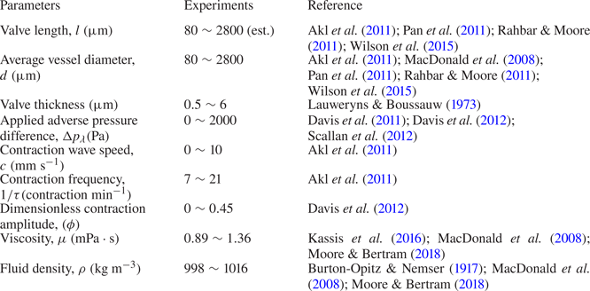
 $\Delta {p_\lambda }$ and the in-plane stiffness and the bending stiffness of the valve. The ranges of these system parameters are selected based on the available experimental data summarized in table 1.
Lymphatic system parameters.

Note that, in lymphatic systems, the contraction amplitude depends on the adverse pressure difference  $\Delta {p_\lambda }$ (Davis et al. Reference Davis, Scallan, Wolpers, Muthuchamy, Gashev and Zawieja2012). Here, we first examine the flow where the two parameters are independent to isolate the effect of each parameter on the flow. Then, the two parameters are coupled via an experimentally reported relationship and investigated to reveal any difference arising from the coupling.
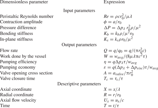
The above mentioned physical parameters can be expressed in terms of the following dimensionless parameters relevant to peristaltic pumping (Shapiro et al. Reference Shapiro, Jaffrin and Weinberg1969; Takabatake et al. Reference Takabatake, Ayukawa and Mori1988), which are indicated using uppercase. We use the dimensionless axial coordinate  $X = x/\lambda $, radial coordinate
 $R = r/{r_0}$, axial component of flow velocity
 ${U_x} = {u_x}/c$ and time
 $T = t/\tau $. The adverse pressure difference is non-dimensionalized as
 $\mathrm{\Delta }P = \Delta {p_\lambda }\; r_0^2\rho /{\mu ^2}$, which represents the ratio between the pressure and viscous forces during peristaltic pumping (Shapiro et al. Reference Shapiro, Jaffrin and Weinberg1969; Rao & Usha Reference Rao and Usha1995; Hariharan, Seshadri & Banerjee Reference Hariharan, Seshadri and Banerjee2008; Böhme & Müller Reference Böhme and Müller2013; Tripathi Reference Tripathi2013; Rachid & Ouazzani Reference Rachid and Ouazzani2015). The Reynolds number for peristaltic pumping is defined as
 $Re = \rho cr_0^2/\mu \lambda $, where
 $\rho $ is the fluid density, and
 $\mu $ is the dynamic viscosity (Shapiro et al. Reference Shapiro, Jaffrin and Weinberg1969; Zien & Ostrach Reference Zien and Ostrach1970; Pozrikidis Reference Pozrikidis1987; Takabatake et al. Reference Takabatake, Ayukawa and Mori1988; Connington et al. Reference Connington, Kang, Viswanathan, Abdel-Fattah and Chen2009). Because parameters that describe
 $Re$ are kept constant throughout the work except for c, a change in peristaltic Reynolds number means a corresponding change in contraction wave speed defined by
 $\tau $. We vary
 $Re$ in the range between
 $0.1$ and
 $1.4$. The dimensionless valve leaflet in-plane and bending stiffnesses are
 ${K_s} = {k_s}\rho {r_0}/{\mu ^2}$ and
 ${K_b} = {k_b}\rho /{\mu ^2}{r_0}$, respectively. These parameters represent the ratios between, respectively, stretching and bending forces experienced by the valve and the viscous forces applied on the vessel wall.
The pumping performance is quantified in terms of the flow rate q averaged over a wave period  $\tau $, the average work done by the vessel wall
 ${w_{avg}}$, pumping efficiency
 $\eta $ and pumping economy
 $\varepsilon $ that are both evaluated over a wavelength
 $\lambda $ and averaged over a wave period
 $\tau $. To calculate
 ${w_{avg}}$, the work done by the vessel wall is calculated by integrating the hydrodynamic force on the wall over the wall displacement and averaging the work over the wavelength
 $\lambda $ and period
 $\tau $ of the vessel. The pumping efficiency is defined as
 $\eta = q\mathrm{\Delta }{p_\lambda }\tau /{w_{avg}}$ while the pumping economy is defined as
 $\varepsilon = q(\mathrm{\Delta }{p_\lambda } + \mathrm{\Delta }{p_{visc}})\tau /{w_{avg}}$, where
 $\mathrm{\Delta }{p_{visc}}$ is pressure loss due to viscous friction for laminar flow arising at flow rate q in a straight pipe with radius
 ${r_0}$ and length
 $\lambda $. This is expressed as
 $\mathrm{\Delta }{p_{visc}} = q/({\rm \pi} r_0^4/8\mu \lambda )$. Thus, the pumping efficiency represents the relative amount of work done by the vessel that goes into the transporting the fluid against the adverse pressure gradient, whereas the flow economy indicates the proportion of the work that is consumed by the fluid transport and viscous losses. The flow rate is normalized as
 $Q = q/{q_0}$, where
 ${q_0} = {\rm \pi}r_0^2c$ is the flow rate in a rigid pipe with radius
 ${r_0}$ and average flow velocity c. Note that this normalization has been previously used for peristaltic pumping (Shapiro et al. Reference Shapiro, Jaffrin and Weinberg1969; Takabatake et al. Reference Takabatake, Ayukawa and Mori1988). Work done by the vessel wall per wave period is normalized by the corresponding friction loss generated in a rigid pipe with an average flow velocity c using the Hagen–Poiseuille law (Sutera & Skalak Reference Sutera and Skalak1993) and is given by
 $W = {w_{avg}}/(8\mu \lambda {\rm \pi}{c^2}\tau )$. To characterize valve opening, we evaluate the cross-sectional area defined by the free edges of the leaflets
 ${a_{valve}}$, and this is normalized as
 $A = {a_{valve}}/{\rm \pi} r_0^2$. The maximum valve opening
 ${A_{max}}$ is defined as the maximum value of A over a vessel cycle. Furthermore, we examine the dimensionless time that the valve is closed per vessel cycle
 ${T_c} = {\tau _c}/\tau $. Here,
 ${\tau _c}$ is the time that valve remains closed during one vessel period. The valve is considered closed when
 $A < 0.05$. The dimensionless parameters are summarized in table 2.
Definitions of the dimensionless parameters.

The simulations start with a stagnant fluid and continue for at least 5 contraction periods to eliminate the influence of the initial transient. This ensures that the difference in the results between consecutive periods does not exceed 1 %.
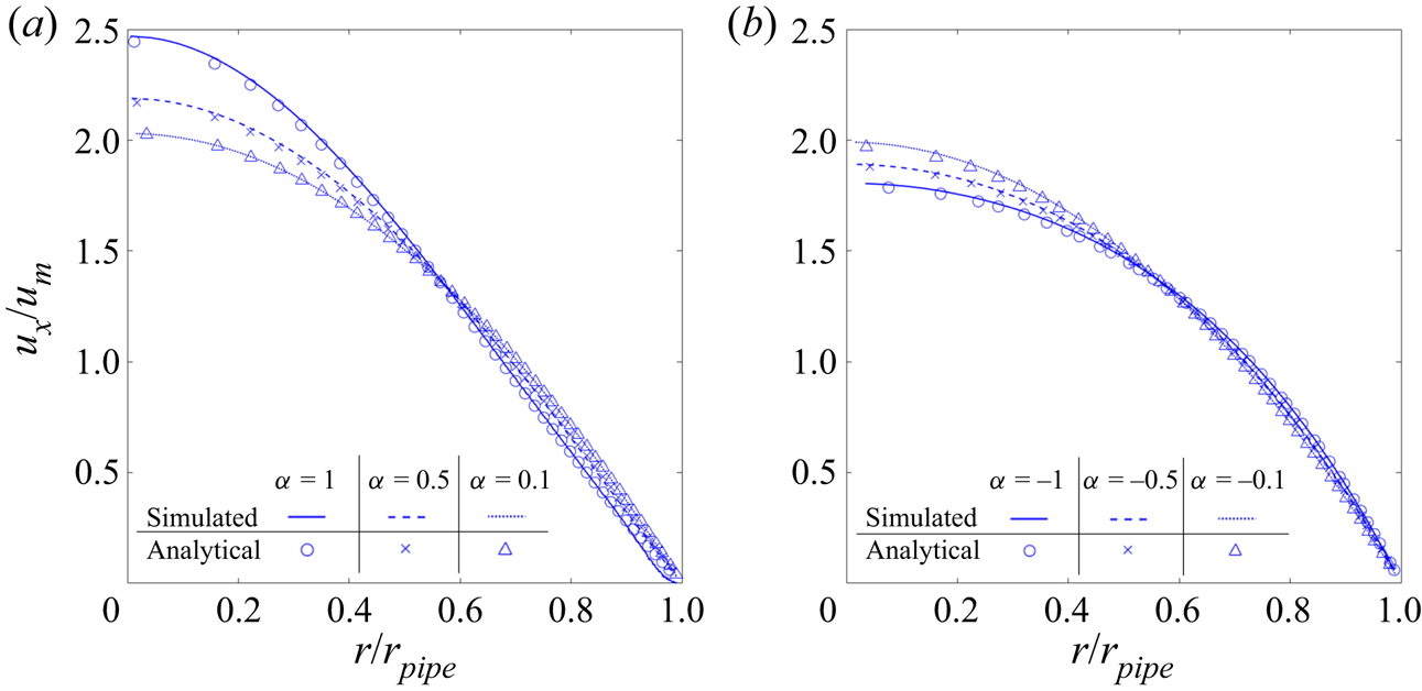
We have previously extensively validated our FSI model with application to different flows including lymphatic pumping (Masoud et al. Reference Masoud, Bingham and Alexeev2012; Mao & Alexeev Reference Mao and Alexeev2014; Yeh & Alexeev Reference Yeh and Alexeev2016; Hanasoge et al. Reference Hanasoge, Ballard, Hesketh and Alexeev2017; Ballard et al. Reference Ballard, Wolf, Nepiyushchikh, Dixon and Alexeev2018). Here, we perform two additional tests to examine the accuracy of the model for simulating flow generated due to moving vessel walls. The first test (figure 3) compares the axial velocity profiles in vessels with radially moving walls with the analytical solutions for semi-infinite circular pipe flow with the same wall motion (Uchida & Aoki Reference Uchida and Aoki1977). The normalized radial velocity is defined as  $\alpha = \rho {v_r}(t)r(t)/\mu $, where
 ${v_r}(t)$ is the radial speed and
 $r(t)$ is the radial position. Three different normalized radial speeds were tested for expanding and contracting vessels. Normalized axial velocity profiles in figure 3 indicate that the numerically calculated flow velocities are in close agreement with the analytical results for both expanding and contracting vessels.
Axial flow velocity  ${u_x}$ in (a) expanding and (b) contracting vessels for different values of radial wall velocity
 $\alpha $. Axial velocity is normalized by the mean axial velocity of the vessel
 ${u_m}$, whereas the radial coordinate r is normalized by the vessel radius
 ${r_{pipe}}$. The lines represent the simulated results, whereas the symbols represent the analytical solution (Uchida & Aoki Reference Uchida and Aoki1977).

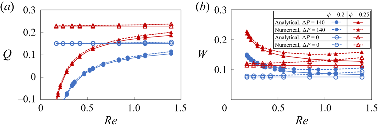
The second test compared Q and W obtained using an analytical solution for peristaltic oscillation (Shapiro et al. Reference Shapiro, Jaffrin and Weinberg1969; Takabatake et al. Reference Takabatake, Ayukawa and Mori1988) with simulated results, as shown in figure 4. The comparison is made for  $\phi = 0.2$ and
 $0.25$,
 $\Delta P = 0$ and
 $140$, and for a range of
 $Re$. It was found that the simulations are close to the analytical solution under different system parameters relevant to our study. Divergence from the analytical solution grows as
 $Re$ increases. This can be expected since the analytical solution assumes
 $Re \ll 1$.
(a) Flow rate Q and (b) vessel work W as a function of peristaltic Reynolds number  $Re$ for different contraction amplitudes
 $\phi $ without valves. The solid and dotted lines show the analytical and numerical solutions, respectively. The empty and filled symbols represent data for
 $\mathrm{\Delta }P = 0$ and
 $\mathrm{\Delta }P = 140$, respectively.

3. Results and discussion
3.1. Flow pattern
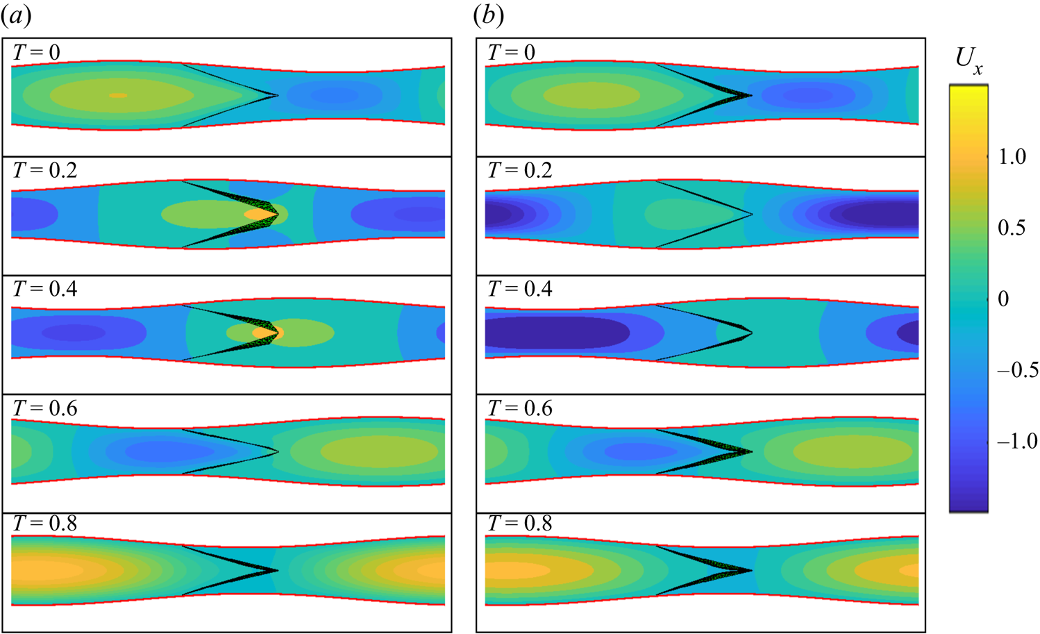
Figures 5(a) and 5(b) present snapshots showing axial velocity and valve deformation for different stages of the vessel contraction cycle without and with an adverse pressure gradient, respectively (see supplementary movie 3). Note that the figures show one valve since the flow profile and valve deformation repeat due to their synchronous motion. Similar to peristaltic pumping without valves (figure 1), the flow is divided into alternating packets of positive and negative axial velocities. Regions of the positive axial velocity travel in the expanded region of the vessel, while packets of negative axial velocity propagate within the contracted region of the vessel. This indicates that velocity packets propagate with the same speed as the contraction wave (Shapiro et al. Reference Shapiro, Jaffrin and Weinberg1969; Takabatake et al. Reference Takabatake, Ayukawa and Mori1988).
(a) Axial flow velocity  ${U_x}$ at different instances of the contraction cycle in a valved vessel with no adverse pressure gradient. (b) Axial flow velocity
 ${U_x}$ in a valved vessel with
 $\mathrm{\Delta }P = 140$. Note that, due to the valves, the flow profile is not axisymmetric. Flow profiles are shown at the symmetry plane perpendicular to the valve opening. The simulation parameters are
 $\phi = 0.2$,
 $Re = 0.2$,
 ${K_b} = 88$ and
 ${K_s} = 115$. See supplementary movie 3 and supplementary movie 4.

Unlike vessels without valves, velocity packets are disrupted when they pass through the elastic valves. Compared to an axisymmetric flow profile in the cases without valves, flow disruption by the valves results in a flow that is no longer axisymmetric even though the pattern of alternating positive and negative velocity packets persists. The valves open when they encounter packets of positive axial velocity and close to occlude the flow when packets of negative axial velocity pass. Thus, the valves affect the forward and backward flow in different ways. While the forward flow is allowed, with some viscous loss due to the reduced orifice size, the backflow can be significantly suppressed and ultimately stopped by fully closed valves.
The valves deform differently when encountering fluid packets with positive and negative velocities, as shown in supplementary movie 4. When encountering packets of positive axial velocity, the leaflets stretch and deform outwards by a combined action of the flow and the vessel expansion. This process increases the opening area of the valve defined by the leaflet free edges, thereby enabling fluid flow. When the valve encounters negative velocity packets, the vessel contracts. The middle of the leaflets deforms inwards, allowing the free edges to rapidly collapse and block the flow. The valve closure process culminates by creating a coaptation zone expanding from the leaflet free edges.
The effect of valves on backflow reduction is more evident when the flow is subjected to an adverse pressure gradient. In this scenario, a peristaltic vessel without a valve has a limited capacity to transport fluid in the direction of wave propagation (figure 1b), whereas the addition of unidirectional valves yields a positive net flow in the vessel (figure 5b). Note that, without an adverse pressure gradient, both vessels with and without valves can successfully pump fluid in the positive direction (figures 1a and 5a). This further points to the important role that valves play in enabling pumping against adverse pressure gradients.
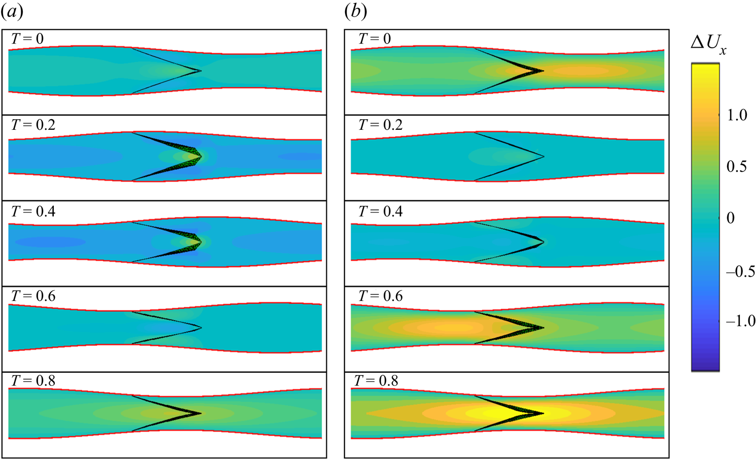
The effect of the valves on pumping is further revealed when considering the difference in axial velocity between vessels with and without valves, denoted as  $\Delta {U_x}$ and shown in figure 6 (see supplementary movie 5). When packets of positive velocity pass through an open valve (see figure 6 for
 $T = 0.2$ and
 $0.4$), the overall flow velocity pattern is similar to the flow in the valve-less vessel with minor flow disturbances around the valves, where the flow accelerates due to the reduced opening between the leaflets. In this case,
 $\Delta {U_x}$ is nearly zero everywhere in the vessel except for a small region in the vicinity of the valve. The velocity difference
 $\Delta {U_x}$ is more significant when vessel contraction passes the valve. In this case, negative flow velocity causes the valve to close and block the flow. This, in turn, results in a positive
 $\Delta {U_x}$ in most of the vessel, as shown in figure 6 for
 $T = 0$, 0.6 and 0.8. A significant positive difference in velocity between the cases with and without valves when the valves are closed indicates that the valves increase pumping by reducing backflow. Furthermore, when comparing figures 6(a) and 6(b), we find that the backflow reduction is more prominent when the pumping is against an adverse pressure gradient. Indeed, the adverse pressure gradient causes a significant negative flow when the valve-less vessel contracts (figure 1b). The backflow is stopped by the closed valves in the case of the vessel fitted with valves (figure 5b).
(a) Axial flow velocity difference  $\Delta {U_x}$ at different instances of the contraction cycle in a valved vessel with no adverse pressure gradient. (b) Axial flow velocity difference
 $\Delta {U_x}$ in a valved vessel with
 $\mathrm{\Delta }P = 140$. Flow profiles are shown at the symmetry plane perpendicular to the valve opening. The simulation parameters are
 $\phi = 0.2$,
 $Re = 0.2$,
 ${K_b} = 88$ and
 ${K_s} = 115$. The flow velocity difference
 $\Delta {U_x}$ is calculated as the difference between flow velocities in vessels with and without valves. See supplementary movie 5.

3.2. Effect of contraction wave speed on pumping
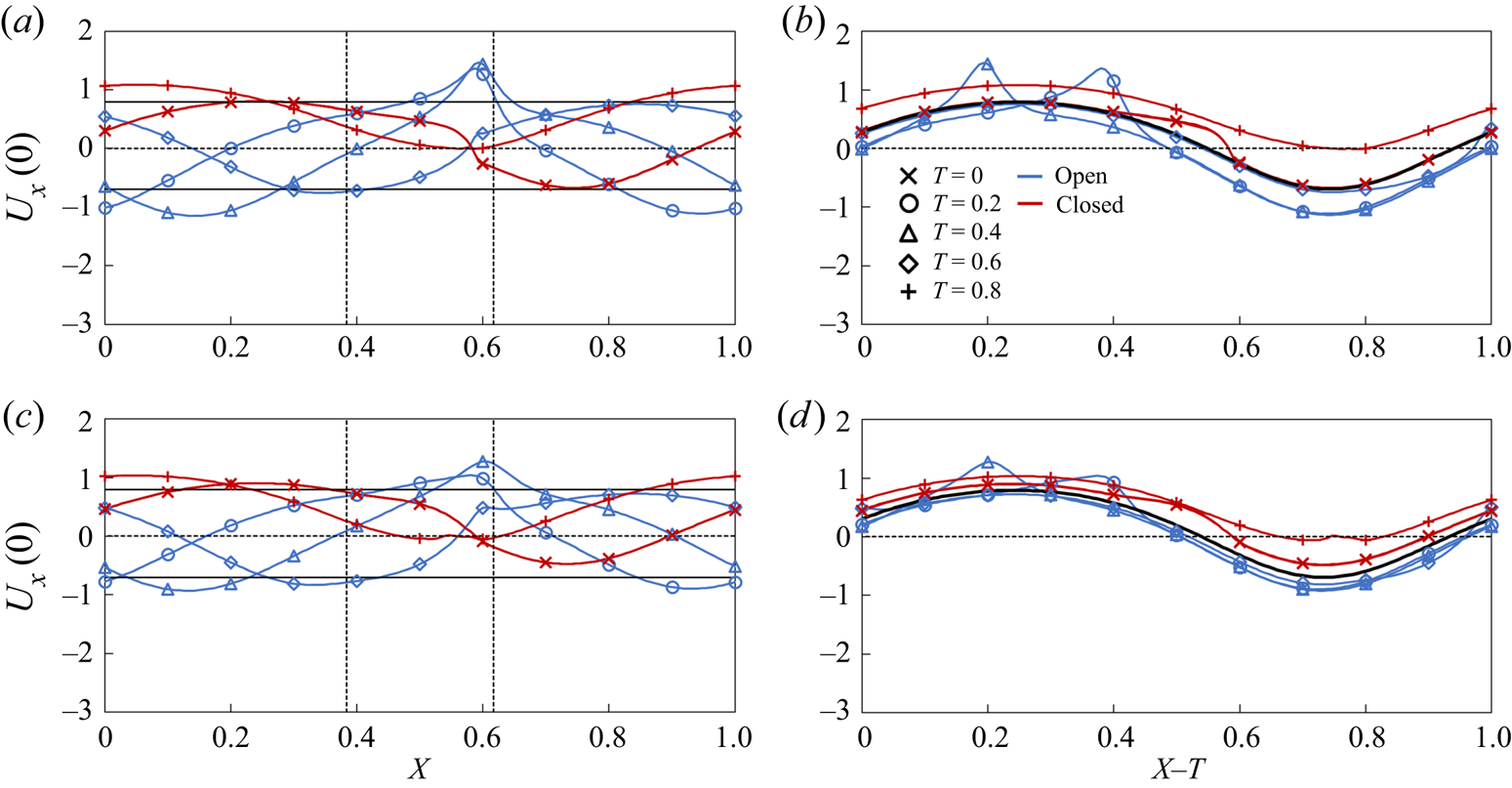
We examine the effect of contraction wave speed on pumping by varying the peristaltic Reynolds number that, in turn, is realized by varying the contraction period  $\tau $. In figure 7, we show how the centreline flow velocity
 ${U_x}(0)$ changes along the vessel without an adverse pressure gradient at
 $Re = 0.2$ and
 $Re = 0.6$. The velocity is shown as a function of the distance along the vessel X and in the moving reference frame
 $X - T$. In figures 7(a) and 7(c), which show the velocity
 ${U_x}(0)$ as a function of the distance along the vessel X, the two vertical dotted lines indicate the location of the valve with the leaflet free edge being on the right side. Furthermore, the horizontal lines in these figures show the maximum and minimum magnitudes of the centreline velocity in a vessel without a valve. Figures 7(b) and 7(d) show the velocity
 ${U_x}(0)$ in the moving reference frame
 $X - T$ in which case the velocity in a valve-less vessel is represented by a single line. Note that the velocities in figures 7(a) and 7(b) correspond to the snapshots shown in figure 5(a).
(a) Centreline axial flow velocity  ${U_x}(0)$ in the stationary reference frame in a vessel with no adverse pressure gradient with
 $Re = 0.2$. The maximum valve opening is
 ${A_{max}} = 0.44$. (b) Same as (a) but in the moving reference frame, the solid black line indicates the average centreline velocity for the valve-less vessel. (c) Centreline axial flow velocity
 ${U_x}(0)$ in a stationary reference frame in a vessel with
 $Re = 0.6$. The maximum opening is
 ${A_{max}} = 0.68$. (d) Same as (c) but in the moving reference frame, the solid black line indicates the average centreline velocity for the valve-less vessel. The horizontal solid lines indicate the maximum and minimum centreline velocities in a vessel without valves. The dashed vertical lines indicate the boundaries of valve position. The blue and red lines show the velocities when the valves are, respectively, open
 $(A \ge 0.05)$ and closed
 $(A < 0.05)$. The simulation parameters are
 $\mathrm{\Delta }P = 0$,
 $\phi = 0.2$,
 ${K_b} = 88$ and
 ${K_s} = 115$.

Outside of the regions around the valve, the centreline velocity follows a sinusoidal wave (figure 7a), which is characteristic of the centreline velocity in peristaltic vessels without valves (figure 1c). The valves introduce a velocity disturbance that is manifested by a local velocity maximum at the valve orifice located at  $X = 0.6$ and is formed by the partially open leaflets at
 $T = 0.2$ and 0.4 (figure 7a). Furthermore, when the valve is closed at
 $T = 0$, 0.6 and 0.8, the centreline velocity between coapted leaflets is nearly zero. Thus, the valve prevents a negative flow at the valve orifice.
To identify the velocity changes induced by the valves with respect to the centreline velocity in the valve-less vessel, we use a moving reference frame that is translated with the speed of the travelling wave (figure 7b). We find that the valve can both decrease and increase the centreline velocity with respect to the valve-less vessel. The velocity corresponding to the open valve condition is somewhat lower than the valve-less velocity. Thus, the flow resistance in the valves on average reduces the flow in the entire vessel. On the other hand, when the valve is closed, the centreline velocity in the vessel exceeds the valve-less velocity. For a fully closed valve, the velocity within the vessel is defined by the fluid redistribution induced by the peristaltic wave propagating along the vessel.
The overall pumping in the vessel with valves is greater than in a valve-less vessel when the backflow reduction due to valve closure outweighs the velocity decrease due to the hydrodynamic resistance in the open valve. Thus, the pumping performance is determined by the valve properties and is maximized when the valve is able to fully block the backflow with minimal resistance for the forward flow.
Increasing the Reynolds number from  $Re = 0.2$ to
 $Re = 0.6$ does not change the general shape of the centreline velocity profile, although the maxima at the valve orifice are less pronounced (figure 7c). During the backflow phase the valve is able to fully close, as indicated by the near zero velocity at
 $T = 0$ and
 $0.8$ at the leaflet edge. Compared to the case of
 $Re = 0.2$, the increase in wave speed decreases the deviation of centreline velocity from that of a valve-less vessel. We also find that the velocity during the open valve phase matches closer to the valve-less velocity with increased Reynolds number, which can be attributed to a reduced hydrodynamic resistance of the valve from a greater opening due to the faster fluid flow. Indeed, at
 $Re = 0.2$, the maximum opening of the valve is approximately 44 % of the cross-sectional area under the average vessel diameter, whereas the maximum opening increases to 68 % when
 $Re = 0.6$.
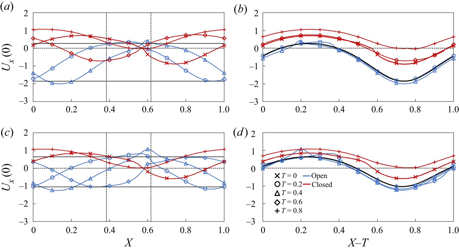
Figure 8 shows centreline velocities for the flow in vessels with  $Re = 0.2$ and
 $Re = 0.6$ that experience an adverse pressure difference
 $\mathrm{\Delta }P = 140$. The velocities in figures 8(a) and 8(b) correspond to the snapshots in figure 5(b). An adverse pressure gradient has a minor effect on the shape of the velocity profiles compared to the case of the flow with
 $\mathrm{\;\ \Delta }P = 0$ (figure 7) although the velocities are shifted towards the negative values. For
 $Re = 0.2$, the valve-less vessel is unable to produce a net positive flow resulting in
 $Q ={-} 0.22$. For the same
 $Re$, the vessel with the valves yields a small positive
 $Q = 0.01$, indicating that a sufficiently high
 $\mathrm{\Delta }P$ can stop pumping by such vessels. Note that further increase of
 $\mathrm{\Delta }P$ leads to the valve remaining fully closed throughout the entire contraction cycle. When compared to the velocity in the valve-less vessel, the velocities at the open valve condition are nearly identical to the valve-less velocity (figure 8b). This can be attributed to a reduced flow through the valve at this
 $\mathrm{\Delta }P$, as shown in figure 8(a).
(a) Centreline axial flow velocity  ${U_x}(0)$ in the stationary reference frame in a vessel with
 $Re = 0.2$ and an adverse pressure gradient. The maximum valve opening is
 ${A_{max}} = 0.3$. (b) Same as (a) but in the moving reference frame, the solid black line indicates the average centreline velocity for the valve-less vessel. (c) Centreline axial flow velocity
 ${U_x}(0)$ in a stationary reference frame in a vessel with
 $Re = 0.6$. The maximum opening is
 ${A_{max}} = 0.61$. (d) Same as (c) but in the moving reference frame, the solid black line indicates the average centreline velocity for the valve-less vessel. The horizontal solid lines indicate the maximum and minimum centreline velocities in vessels without valves. The dashed vertical lines indicate the boundaries of valve position. The blue and red lines show the velocities when the valves are, respectively, open
 $(A \ge 0.05)$ and closed
 $(A < 0.05)$. The simulation parameters are
 $\mathrm{\Delta }P = 140$,
 $\phi = 0.2$,
 ${K_b} = 88$ and
 ${K_s} = 115$.

At a larger  $Re = 0.6$ (figure 8c) both vessels with and without valves are able to generate a net positive fluid flow in spite of an adverse pressure gradient. However, valves enable significantly greater pumping of
 $Q = 0.11$ compared to
 $Q = 0.04$ without valves. This is again due to the ability of valves to stop backflow. The velocity during the open valve phase is slightly lower than the valve-less velocity (figure 8d) and comparable to the velocity in the flow without an adverse pressure gradient (figure 7d). Indeed, in both cases, the normalized maximum valve openings are comparable at 61 % and 68 %, for
 $\mathrm{\Delta }P = 140$ and
 $\mathrm{\Delta }P = 0$, respectively. Thus, this adverse pressure gradient has a rather insignificant effect on the maximum valve opening.
Note that increasing  $Re$ has opposing effects on the peristaltic pumping with valves. On one hand, increasing
 $Re$ facilitates valve opening and decreases the associated viscous loss; on the other hand, the time during which the valve is closed decreases impairing the valve's ability to fully arrest the backflow. Indeed, at
 $Re = 0.2$ the valve is closed approximately 62 % of the contraction cycle, whereas at
 $Re = 0.6$ the valve is closed approximately 42 % of the contraction cycle.
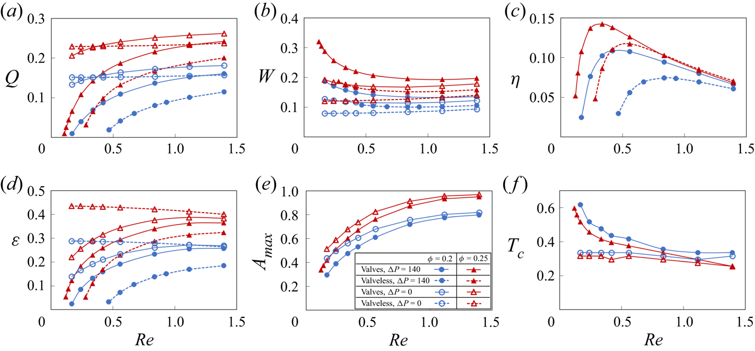
The dependencies of the pumping parameters on  $Re$ are summarized in figure 9. The data are shown for
 $\mathrm{\Delta }P = 0$ using the empty symbols, and for
 $\mathrm{\Delta }P = 140$ using the filled symbols. Figure 9(a) shows that normalized flow rate Q mostly increases as
 $Re$ increases. Without an adverse pressure gradient, Q remains nearly flat in valve-less vessels and slightly increases when vessels are fitted with valves. Thus, the flow rate has a nearly linear relationship with the wave speed. When the pumping occurs against an adverse pressure gradient, Q rapidly decreases with decreasing
 $Re$. Without valves, low
 $Re$ results in a negative Q, meaning that peristaltic pumping cannot overcome the adverse pressure gradient at these wave speeds. With valves, however, low
 $Re$ leads to slightly positive values of Q, indicating that, whereas peristatic motion cannot pump the fluid, the valves are able to eliminate the backflow.
(a) Flow rate, (b) vessel work, (c) pumping efficiency, (d) pumping economy, (e) maximum valve opening area  ${A_{max}}$ and (f) valve closure time
 ${T_c}$ as a function of peristaltic Reynolds number for vessels with
 ${K_b} = 88$ and
 ${K_s} = 115$. The empty and filled symbols represent data
 $\mathrm{\Delta }P = 0$ and
 $\mathrm{\Delta }P = 140$, respectively. The dashed lines represent results from valve-less vessels. The valve is considered closed when
 $A < 0.05$.

Figure 9(b) shows the normalized work W done over a wave period by the peristaltic vessel. In valve-less cases and in valved cases with  $\mathrm{\Delta }P = 0$, W is nearly constant, indicating that the work done by the vessel increases nearly quadratically with
 $Re$ since the normalization factor is proportional to
 $R{e^2}$. Otherwise, the work W decreases with increasing
 $Re$, as an increased flow rate leads to a larger valve opening and decreased loss from valve interference with the flow.
Pumping efficiency  $\eta = q\mathrm{\Delta }{p_\lambda }/{w_{avg}}$ is shown in figure 9(c) as a function of
 $Re$. The efficiency is defined as the ratio between the work due to the fluid transport against the adverse pressure gradient and the work done by the vessel. Note that, when
 $\mathrm{\Delta }P = 0$, the efficiency is zero. We therefore present data only for
 $\mathrm{\Delta }P = 140$. We find that the efficiency curves for vessels with and without valves exhibit maxima, indicating the existence of an optimum
 $Re$ maximizing the pumping per unit work against an adverse pressure gradient. This result is consistent with the analytical solution for peristaltic pumping (Shapiro et al. Reference Shapiro, Jaffrin and Weinberg1969; Takabatake et al. Reference Takabatake, Ayukawa and Mori1988). The maxima of efficiency are a result of two opposing trends. At small
 $Re$, peristaltic pumping cannot overcome the adverse pressure gradient diminishing the flow rate and therefore the pumping efficiency. For higher
 $Re$, the flow rate increases as
 $Re$, whereas the work increases as
 $R{e^2}$, leading to overall efficiency decrease with
 $Re$. Interestingly, valves increase the maximum efficiency and shift it to the lower values of
 $Re$. This can be related to a more rapid decrease of the flow rate with decreasing
 $Re$ in valve-less vessels due to the adverse pressure gradient compared to vessels fitted with valves. Furthermore, the efficiency is greater for larger
 $\phi $ as a result of a faster flow (figure 9a). For larger
 $Re$, the efficiency of valve-less and valved vessels nearly overlaps, indicating a weak effect of valves on pumping in this flow regime.
Another metric to characterize the performance of the peristaltic pumping is the flow economy,  $\varepsilon $, shown in figure 9(d) as a function of
 $Re$. In addition to accounting for the work against the adverse pressure gradient, as is in the case for
 $\eta $,
 $\varepsilon $ also accounts for the viscous losses in the vessel. We find that
 $\varepsilon $ is significantly greater than
 $\eta $ and closely resembles the trend of the normalized flow rate shown in figure 9(a), indicating that a greater amount of work by the vessel goes to viscous loss than to pumping the fluid. Without an adverse pressure gradient,
 $\varepsilon $ for the valve-less vessel exceeds the value for vessels with valves, due to the additional loss associated with valves restricting the flow. The difference decreases with increasing
 $Re$ due to the larger valve opening (figure 9e). However, when
 $\mathrm{\Delta }P = 140$,
 $\varepsilon $ for vessels with valves exceeds the valve-less
 $\varepsilon $. Thus, adding valves improve the economy when the flow is confronted by an adverse pressure gradient, whereas without an adverse pressure, pumping of the valve-less vessel is more economical.
We further characterize valve behaviour during peristaltic pumping by quantifying the maximum valve opening area  ${A_{max}}$ and the occlusion time
 ${T_c}$, which are shown as a function of
 $Re$ in respective figures 9(e) and 9(f). The maximum opening area steadily increases with
 $Re$ and plateaus for
 $Re > 1$. For lower
 $Re$, an adverse pressure gradient somewhat decreases
 ${A_{max}}$ as a result of a lower positive flow velocity in the vessel (figure 8). The occlusion time
 ${T_c}$ is relatively constant with
 $Re$ when the flow is not affected by
 $\mathrm{\Delta }P$. This is consistent with the velocity profiles shown in figure 7 that exhibit minor variations for different
 $Re$. On the other hand, an adverse pressure gradient causes
 ${T_c}$ to increase with decreasing
 $Re$, as longer occlusion period occurs due to the increased backflow.
3.3. Effect of adverse pressure gradient on pumping
Figure 10 presents the dependence of peristaltic pumping parameters for vessels with and without valves on the magnitude of the adverse pressure difference  $\mathrm{\Delta }P$. Here, we keep the wave speed constant, leading to
 $Re = 0.4$. We find that the normalized flow rate Q decreases linearly with increasing
 $\mathrm{\Delta }P$ (figure 10a). Furthermore, Q increases with wave amplitude
 $\phi $. For vessels without valves the decrease of Q is more rapid than for vessels with valves. As a result, valved vessels are able to pump fluid against significantly greater
 $\mathrm{\Delta }P$. However, this enhanced pumping in valved vessels comes at the cost of increased work W performed by the vessel (figure 10b). The work by vessels with valves exceeds the work by valve-less vessels likely due to the increased viscous losses associated with the flow through the occluding valves. Increased wave amplitude
 $\phi $ results in greater W.
(a) Flow rate, (b) vessel work, (c) pumping efficiency, (d) pumping economy, (e) maximum valve opening area  ${A_{max}}$ and (f) valve closure time
 ${T_c}$ as a function of adverse pressure difference
 $\mathrm{\Delta }P$ for vessels with
 $Re = 0.4$,
 ${K_b} = 88$ and
 ${K_s} = 115$. The dashed lines represent results from valve-less cases. The valve is considered closed when
 $A < 0.05$.

Pumping efficiency is presented in figure 10c. In spite the greater work done by vessels with valves, their efficiency is either comparable (at lower  $\mathrm{\Delta }P$) or exceeds (at higher
 $\mathrm{\Delta }P$) that of valve-less vessels. Thus, in terms of pumping efficiency, the greater pumping capacity overcomes the increased viscous loss created by the valves. Furthermore, pumping efficiency curves exhibit maxima, indicating the existence of optimum values of the adverse pressure gradient leading to the most efficient peristaltic pumping. For a vessel with valves, the optimum
 $\mathrm{\Delta }P$ significantly exceeds that for a valve-less vessel. Furthermore, increasing
 $\phi $ increases the efficiency and the optimum
 $\mathrm{\Delta }P$. Thus, by changing vessel parameters the pumping can be optimized to a specific value of
 $\mathrm{\Delta }P$.
Flow economy shows nearly linear decrease with  $\mathrm{\Delta }P$ (figure 10d). At lower
 $\mathrm{\Delta }P$, the work of vessel contraction mostly goes to overcome viscous friction loss rather than useful pumping. At these conditions,
 $\varepsilon $ for valve-less vessels exceeds
 $\varepsilon $ for vessels with valves. At higher
 $\mathrm{\Delta }P$, vessels with valves exhibit better economy than valve-less vessels. Note that the economy is greater when the wave amplitude is increased.
The maximum valve opening area and valve occlusion time are shown in figures 10(e) and 10(f), respectively. Increasing adverse pressure gradient gradually decreases the valve maximum opening and increases the time that valve stays closed per contraction cycle. That is consistent with the reduction of the pumping flow rate with increasing  $\mathrm{\Delta }P$ (figure 10a). Indeed, the slower flow velocity and lower favourable pressure gradient in the vessel decrease the forces acting to open the elastic valve resulting in lower
 ${A_{max}}$ and longer
 ${T_c}$.
3.4. Effect of valve elastic properties on pumping
Figure 11 shows the side views of the valves at three representative bending stiffnesses, which we further refer as soft, normal and stiff valves (see supplementary movie 6). The valves are plotted at different instances of vessel operation. Figure 11(a) indicates that soft valves experience valve depression at the middle of the valve under backflow. This deformation does not prevent backflow until the valve free ends fully close. Normal and stiff valves in figures 11(b) and 11(c) experience closures at the valve free ends, leading to a more effective backflow prevention than the soft valve. However, stiff valves are less responsive to changing flow rate, lengthening the time required for the valve to be fully open and closed, decreasing the maximum valve opening area during the forward flow and increasing the time the valve remains closed after the flow reversal.
(a) Deformation of valves with  ${K_b} = 11$, (b) with
 ${K_b} = 88$, (c) with
 ${K_b} = 263$ at different instances of the vessel contraction cycle. The dots represent leaflet position at the centreline. The simulation parameters are
 $\mathrm{\Delta }P = 140$,
 $\phi = 0.2$,
 $Re = 0.4$ and
 ${K_s} = 115$. See supplementary movie 6.

The behaviour of the elastic valves can be further characterized by analysing the time evolution of the flow rate  ${Q_s}$ and the leaflet cross-sectional opening area A that are shown in figure 12 for flow with and without an adverse pressure gradient. The flow rate
 ${Q_s}$ is averaged over the entire simulation domain. Note that, for a valve-less vessel,
 ${Q_s}$ remains constant, as shown by the dashed lines in figures 12(a) and 12(c). Figures 12(b) and 12(d) also show the vessel radius at the valve location.
(a) Time evolution of flow rate in vessels with  $\mathrm{\Delta }P = 0$. (b) Time evolution of valve opening area A in vessels with
 $\mathrm{\Delta }P = 0$. Panels (c) and (d) are the same as (a) and (b) but with
 $\mathrm{\Delta }P = 140$. The flow rate is averaged over contraction wavelength. The horizontal dashed line represents flow rate in the valve-less vessel while the dotted lines in (b,d) represent normalized vessel radius near the valve
 $(r/{r_0})$. Dashed lines in (a,c) indicate when
 $r/{r_0} > 1$ while solid lines indicate
 $r/{r_0} < 1$. Horizontal dash-dot lines in (a,c) denote
 ${Q_s} = 0$. The simulation parameters are
 $\phi = 0.2$,
 $Re = 0.4$ and
 ${K_s} = 115$.

The valves open when the vessel diameter at the valve location increases (figures 12b and 12d), which corresponds to the forward fluid flow through the valve (figure 5). The valve opening is maximized when the vessel diameter is near its mean value. Softer valves can open more widely during flow through the valve and stay open longer. Furthermore, for such valves the opening starts later than for stiffer valves. Comparing the flow with and without an adverse pressure gradient, we find that the adverse pressure gradient suppresses valve opening with the effect being more significant for softer valves. This can be attributed to the lower flow velocity and favourable pressure gradient for valve opening when the flow is affected by an adverse pressure.
The valve kinematics strongly affects the flow rate in the vessel (figures 12b and 12d). When the valves are open, softer valves impose lower resistance on the flow leading to a faster flow. However, even with the softest valve, the instantaneous flow rate with an open valve is slower than in the case of a valve-less vessel. When the valves are closed, the flow rate increases and exceeds the valve-less flow rate. Stiffer valves that close sooner enable a larger mean flow rate. Thus, during the oscillation period, the fluid is mostly pumped when the valves are closed, and the fluid is transported by the contracting wave propagating along the vessel. This behaviour is more evident when the flow is confronted with an adverse pressure gradient (figure 12c). In this case, the flow rate is negative when the valves are open, and the fluid is transported in the positive direction only when the valves are closed. Note that for the same adverse pressure gradient valve-less vessel generates a nearly zero net flow.
We therefore conclude that valve elasticity has opposing effects on the pumping performance. Softer valves enable greater valve opening, reducing viscous losses when the flow is moving in the positive direction through the valve. On the other hand, stiffer valves can close more rapidly during backflow, minimizing flow reversal during this phase. This indicates that an optimum value of elasticity exists that maximizes the vessel pumping performance.
Figure 13 presents the pumping parameters as a function of valve bending elasticity  ${K_b}$ for vessels with
 $\mathrm{\Delta }P = 140$ and two wave amplitudes
 $\phi = 0.2$ and
 $\phi = 0.25$. We indeed find that the flow rate is maximized when
 ${K_b} \approx 63$ (figure 13a). This optimum bending elasticity is approximately the same for both contraction wave amplitudes. The pumping efficiency and economy (figures 13c and 13d) also exhibit maxima with
 ${K_b}$. Here, the optimum elasticity
 ${K_b} \approx 50$ is somewhat lower than that for the maximum flow rate.
(a) Flow rate, (b) vessel work, (c) pumping efficiency, (d) pumping economy, (e) maximum valve opening area  ${A_{max}}$ and (f) valve closure time
 ${T_c}$ as a function of valve bending stiffness
 ${K_b}$ for vessels with
 $\mathrm{\Delta }P = 140$ and
 $Re = 0.4$. The dashed lines represent results from valve-less cases. The valve is considered closed when
 $A < 0.05$.

We also find that work done by the vessel W gradually increases with increasing  ${K_b}$ (figure 13b). The work increase is related to the higher viscous losses associated with less deformable valve leaflets (Ballard et al. Reference Ballard, Wolf, Nepiyushchikh, Dixon and Alexeev2018) that exhibit a lower valve opening area (figure 13e). These figures show that this trend is independent of the wave amplitude. While
 ${A_{max}}$ steadily decreases with increasing
 ${K_b}$, the time the valve stays closed
 ${T_c}$ is nearly independent of
 ${K_b}$ for
 ${K_b} > 50$, and sharply decreases for lower
 ${K_b}$. This indicates that softer valves are unable to properly close and fail to prevent the backflow in the vessel.
In figure 13, we also examine the effect of the leaflet in-plane stiffness  ${K_s}$ on the valve performance. We compare valves with
 ${K_s} = 23$, 115 and 575. We find that a nearly 25-fold change of in-plane stiffness has a minor effect on the vessel parameters such as flow rate Q, work done by the vessel W, efficiency
 $\eta $ and economy
 $\varepsilon $. Only a slight decrease of
 ${A_{max}}$ is found for the valves with
 ${K_s} = 575$ compared to the less stiff valves. Interestingly, the time that valve is closed
 ${T_c}$ is practically insensitive to changes in
 ${K_s}$. Thus, we conclude that the valve behaviour is mostly defined by the valve bending elasticity whereas in-plane stiffness plays a minor role.
The emergence of an optimum  ${K_b}$ indicates that the valve mechanical properties can be optimized for specific pumping conditions. Furthermore, the optimum
 ${K_b}$ leading to the fastest pumping performance and the highest efficiency and economy are somewhat different due to the dependency of W on
 ${K_b}$. Indeed, increasing W with
 ${K_b}$ results in the softer valve being more efficient while providing slightly slower pumping. In figure 14, we examine the dependency of the optimum valve elasticity on the magnitude of the adverse pressure gradient. The figure shows that the optimum elasticity increases with
 $\Delta P$. We relate this trend to the improved ability of stiffer valves to withstand backflow due to an increasing adverse pressure gradient as such valves can close faster than softer valves (figure 12d). When
 $\Delta P$ increases, the flow rate in the vessel reduces and the ability to prevent the backflow has a more significant effect on the pumping than increased viscous losses due to stiffer valves.
Optimal normalized bending stiffness yielding the maximum efficiency, economy and flow rate under different adverse pressure gradients. The simulation parameters are  $\phi = 0.2$,
 $Re = 0.4$ and
 ${K_s} = 115$.

3.5. Effect of contraction amplitude dependence on adverse pressure gradient
In the lymphatic system, the vessel contraction amplitude depends on the magnitude of the adverse pressure gradient (Davis et al. Reference Davis, Scallan, Wolpers, Muthuchamy, Gashev and Zawieja2012). As shown in figure 15, contraction amplitude gradually decreases with increasing  $\Delta P$. The decrease is more rapid for lower
 $\Delta P$ and the amplitude converges to a non-zero value when the pressure gradient increases beyond
 $\Delta P > 1000$ due to the inability of the lymphatic muscle cells to generate enough force for the pressure in the vessel proximal to the valve to exceed the pressure distal to the valve.
Contraction amplitude as a function of normalized pressure difference. Experimentally reported values (Davis et al. Reference Davis, Scallan, Wolpers, Muthuchamy, Gashev and Zawieja2012) are shown by the triangles while the fit is shown by the solid line.

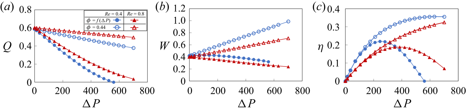
In figure 16, we examine the effects of the pressure dependence of the contraction amplitude on the pumping performance. To isolate these effects, we compare the normalized flow rate Q, work done by the vessel  $W$ and pumping efficiency
 $\eta $ for a vessel with pressure-dependent contraction amplitude to a vessel with a constant contraction amplitude. For the later vessel, we set the contraction amplitude such that the amplitudes for both vessels are identical when
 $\Delta P = 0$. The data are presented for two values of
 $Re$.
(a) Flow rate, (b) vessel work and (c) pumping efficiency as a function of the pressure gradient for vessels with and without a pressure-dependent contraction amplitude. The valve elasticity is  ${K_b} = 88$ and
 ${K_s} = 115$. Without an adverse pressure gradient both vessels exhibit an identical contraction amplitude of
 $\phi = 0.44$.

The simulations show that vessels with pressure-dependent amplitude significantly underperform compared to the constant amplitude vessels, resulting in a rapid decrease of the pumping flow rate with increasing adverse pressure gradient (figure 16a). This trend is consistent with the results shown in figure 10(a), indicating a reduction in pumping rate with lower contraction amplitude. Pressure-dependent contraction amplitude also has significant effect on the work done by the pumping vessel. As shown in figure 16b, constant contraction amplitude leads to an increasing amount of work as the adverse pressure increases. By contrast, the pressure-dependent amplitude results in work that is nearly independent of  $\Delta P$. This result suggests that the lymphatic vessel contraction amplitude is limited by the work of contractile muscles driving vessel contraction and that, once exposed to an adverse pressure gradient, lymphatic muscle quickly achieves maximum capacity in terms of the work generated. It is also interesting to note that the work only slightly changes with
 $Re$. Furthermore, a pressure-dependent contraction amplitude decreases the pumping efficiency compared to the constant amplitude case (figure 16c). Although the work is roughly constant with pressure, the decreasing Q in the pressure-dependent vessels results in a rapid decrease in efficiency when
 $\Delta P$ is sufficiently large. As a result, the optimum pumping occurs at lower values of
 $\Delta P$ compared to the vessels with a constant contraction amplitude.
4. Summary
Using fully coupled three-dimensional simulations, we investigate fluid pumping by a peristaltic vessel outfitted with elastic valves. The valves are formed by two adjusted angled elastic sheets representing a typical valve in a collecting lymphatic vessel. We compare fluid pumping by peristaltic vessels with and without valves to identify and isolate the effects of the valves on the resulting flow rate and pumping performance characterized in terms of pumping efficiency and economy. The simulations show that elastic valves increase the net fluid flow generated by a peristaltic vessel by reducing the backflow due to the periodic vessel contractions. At the same time, valves generate an additional flow resistance during the forward fluid flow. The effect of the valves on the pumping is more pronounced at lower Reynolds numbers and when the pumping is performed against an adverse pressure gradient. In both scenarios, the pumping by a valve-less peristaltic vessel diminishes due to a significant backflow.
We systematically investigate the effects of the vessel contraction wave speed, contraction amplitude, adverse pressure gradient and valve elastic properties on the pumping performance. Increased vessel contraction wave speed and contraction amplitude increase pumping flow rate and work done by the vessel. Increasing the adverse pressure gradient suppresses fluid pumping while requiring greater work by the vessel. The valve stiffness exhibits an optimum maximizing the pumping flow rate. Higher valve stiffness increases the viscous loss leading to an increased work, whereas softer valves close slowly, enhancing backflow. The pumping economy is dominated by the viscous losses in the vessel and, thus, increases with increasing pumping flow rate. Optimal valve and vessel parameters exist that maximize the pumping efficiencies of valved peristaltic vessels. We find that the stiffer valves are required with increased adverse pressure gradients to maintain the high pumping efficiency. When the vessel contraction amplitude decreases with increasing adverse pressure gradient in the manner in which it takes place in lymphatic systems, we find that vessel maintains a relatively constant work for the entire range of pressure gradient, while gradually decreasing the pumping flow rate. This result indicates that lymphatic vessel pumping is limited by the contractile capacity of the lymphatic muscle.
Understanding valve mechanics in the lymphatic vasculature has become increasingly important. Oscillatory wall shear stress has been shown to enhance the expression of transcription factors necessary for the formation of lymphatic valves during development as well as for post-natal valve maintenance (Sabine et al. Reference Sabine, Agalarov, Maby-El Hajjami, Jaquet, Hägerling, Pollmann, Bebber, Pfenniger, Miura and Dormond2012, Reference Sabine, Bovay, Demir, Kimura, Jaquet, Agalarov, Zangger, Scallan, Graber and Gulpinar2015; Cha et al. Reference Cha, Geng, Mahamud, Fu, Mukherjee, Kim, Jho, Kim, Kahn and Xia2016, Reference Cha, Geng, Mahamud, Zhang, Chen, Kim, Jho, Kim, Choi and Dixon2018; Choi et al. Reference Choi, Park, Jung, Cha, Lee, Yu, Kim, Lee, Hong and Koh2019). In addition, mutations in mouse models in genes associated with primary lymphedema have produced valves that are dysfunctional at preventing backflow (Lapinski et al. Reference Lapinski, Kwon, Lubeck, Wilkinson, Srinivasan, Sevick-Muraca and King2012, Reference Lapinski, Lubeck, Chen, Doosti, Zawieja, Davis and King2017; Kazenwadel et al. Reference Kazenwadel, Betterman, Chong, Stokes, Lee, Secker, Agalarov, Demir, Lawrence and Sutton2015; Castorena-Gonzalez et al. Reference Castorena-Gonzalez, Srinivasan, King, Simon and Davis2020) and abnormal conduction of contraction waves (Castorena-Gonzalez et al. Reference Castorena-Gonzalez, Zawieja, Li, Srinivasan, Simon, de Wit, de la Torre, Martinez-Lemus, Hennig and Davis2018). Thus, understanding the structure–function relationships that underpin proper valve performance and how subtle alterations in lymphatic structure and mechanics negatively impact lymphatic transport is of high clinical importance. Moreover, knowledge of these structure–function relationships could also provide insight into the underlying mechanobiology that is driving the observed regional variation in lymphatic vessel pumping behaviour and morphology (Gashev et al. Reference Gashev, Davis, Delp and Zawieja2004, Reference Gashev, Zhang, Muthuchamy, Zawieja and Davis2012; Zawieja et al. Reference Zawieja, Castorena-Gonzalez, Scallan and Davis2018). For example, it is possible that the regional differences in valve length and morphology in vessels close to the heart (such as the thoracic duct) compared to vessels found in the extremities could exist to optimize function in the context of the local mechanical loads placed on these vessels. Finally, our findings from this study can lead the development of simplified functional relationships between various valve properties and flow performance metrics, which can be incorporated into the existing lower-dimensional models. Such simplified models are computationally less expensive, enabling simulations of extensive lymphangion chains and their branched networks.
Supplementary movies
Supplementary movies are available at https://doi.org/10.1017/jfm.2021.302.
Funding
The work was supported by the National Science Foundation (CMMI-1635133) and National Institutes of Health (1R01HL152152-01).
Declaration of interests
The authors report no conflict of interest.