1 Introduction
Roughness-induced transition has been a subject of extensive study dating back to the 1940s (Dryden Reference Dryden1953). Understanding the role of roughness in flow transition is essential for prediction and design, as well as flow control and drag reduction through the delay of the turbulent transition (Cossu & Brandt Reference Cossu and Brandt2002; Choi Reference Choi2006; Fransson et al.
Reference Fransson, Talamelli, Brandt and Cossu2006). Early works focused on the roughness Reynolds number
 $Re_{k}=U_{k}k/\unicode[STIX]{x1D708}$
as a characteristic parameter in determining the transition (e.g., Klebanoff, Schubauer & Tidstrom Reference Klebanoff, Schubauer and Tidstrom1955; Smith & Clutter Reference Smith and Clutter1959); here,
 $U_{k}$
denotes the velocity at the roughness height (
 $k$
) and
 $\unicode[STIX]{x1D708}$
is the kinematic viscosity. Further distinctions are based on whether the roughness is two-dimensional (2D) or three-dimensional (3D), and whether it is distributed or isolated. In terms of
 $Re_{k}$
, the transition to turbulence is expected to occur downstream of the roughness element at a critical threshold
 $Re_{k,crit}$
. Moreover, a 3D roughness is identified as more critical than a 2D one, meaning that when
 $Re_{k,crit}$
has been exceeded, the transition location will rapidly approach the roughness element (Tani Reference Tani1969). Below
 $Re_{k,crit}$
, it was believed that 3D roughness has an insignificant effect on the flow transition (Klebanoff et al.
Reference Klebanoff, Schubauer and Tidstrom1955; Tani Reference Tani1969).
As discussed by Klebanoff & Tidstrom (Reference Klebanoff and Tidstrom1972), Ergin & White (Reference Ergin and White2006), Kuester & White (Reference Kuester and White2015) and others, the
 $Re_{k}$
criterion falls short in explaining the underlying physics of the transition process. Understanding roughness-induced transition is an essential prerequisite to the use of roughness as a control mechanism to reduce skin friction by delaying the flow transition, as proposed by Shahinfar et al. (Reference Shahinfar, Sattarzadeh, Fransson and Talamelli2012, Reference Shahinfar, Fransson, Sattarzadeh and Talamelli2013) and others. For discrete 2D roughness, the transition is explained by the 2D Tollmien–Schlichting (T–S) waves (Klebanoff & Tidstrom Reference Klebanoff and Tidstrom1972; Goldstein Reference Goldstein1985). The need for further understanding of the effect of 3D roughness on flow transition has motivated many recent studies, including Bernardini et al. (Reference Bernardini, Pirozzoli, Orlandi and Lele2014), Plogmann, Würz & Krämer (Reference Plogmann, Würz and Krämer2014), Edelmann & Rist (Reference Edelmann and Rist2015) and Ye, Schrijer & Scarano (Reference Ye, Schrijer and Scarano2016), to name a few. Transient growth, a candidate mechanism explaining bypass transition over 3D isolated and distributed roughness, emerges due to the non-orthogonality of the linear stability equations (Reshotko Reference Reshotko2001; Reshotko & Tumin Reference Reshotko and Tumin2004; Downs, White & Denissen Reference Downs, White and Denissen2008). Essentially, it is described by the combination of slightly decaying modes, resulting in transient growth followed by exponential decay (Reshotko & Tumin Reference Reshotko and Tumin2004; Kuester & White Reference Kuester and White2015).
Recent works have focused on the flow in the near and far wake of 3D isolated roughness elements. Ergin & White (Reference Ergin and White2006), for example, studied the flow past an array of cylindrical elements at subcritical and supercritical
 $Re_{k}$
. In addition to providing evidence of hairpin vortices, they highlighted that the transition occurs when the field of the unsteady disturbance (velocity fluctuations) grows rapidly such that the altered steady flow cannot relax fast enough to stabilize the fluctuations. As such, roughness-induced transition could be thought of as a competition between these two factors. Recently, Ye et al. (Reference Ye, Schrijer and Scarano2016) experimentally investigated the transition past a micro-ramp at a supercritical
 $Re_{k}=1170$
using tomographic particle image velocimetry (PIV) and highlighted the shedding of arc-like Kelvin–Helmholtz (K–H) vortices. Past the breakup of the arc-like vortices, a region of relatively low vortical activity was observed, followed by the development of hairpin vortices near the wall, indicating flow transition.
The role of distributed roughness in flow transition remains a challenging topic in need of further investigation, especially due to its relevance as a realistic wall condition. Downs et al. (Reference Downs, White and Denissen2008) studied the flow transition past a patch of random distributed roughness at
 $Re_{k}=164$
, 227 and 301. They observed transient growth in the steady disturbances (deviations from the Blasius profile due to the generated wakes) across the three
 $Re_{k}$
, and suggested that the transition at the high
 $Re_{k}$
occurs through bypass mechanisms. Moreover, they observed a similar competition between the relaxation of steady disturbances (stabilizing effect) and the growth of the fluctuations as in Ergin & White (Reference Ergin and White2006). Direct numerical simulations (DNS) of the flow past the same roughness were performed by Drews et al. (Reference Drews, Downs, Doolittle, Goldstein and White2011) and Drews (Reference Drews2012) to further understand the nature of the transition. A key finding in these works is that the regions with the largest roughness heights were responsible for the majority of the distortion of the initially undisturbed boundary layer. Additionally, Drews (Reference Drews2012) suggested that the small roughness acts as a ‘shield’ where the boundary layer gets displaced vertically over the small-scale roughness, thus shielding the larger roughness elements through a lower effective
 $Re_{k}$
. Because of the importance of such an effect, Kuester & White (Reference Kuester and White2015) performed systematic experiments to investigate the nature of the interaction between distributed roughness and isolated elements. They found that sheltering is not fully explained by boundary layer displacement as suggested by Drews (Reference Drews2012).
The works of Downs et al. (Reference Downs, White and Denissen2008) and Kuester & White (Reference Kuester and White2015) pointed out the need for a characterization of flow transition over long patches of distributed roughness. Our study aims to contribute to satisfying this need within the rapidly evolving field of roughness-induced transition. Here, we consider the transition to turbulence over 2D and 3D wavy walls. The flow over these roughnesses in the regime of developed turbulence has been studied by Hamed et al. (Reference Hamed, Kamdar, Castillo and Chamorro2015), who found that 3D roughness led to reduced drag in comparison to the 2D case. This reduction was attributed to the characteristic spanwise flows within the 3D wall, which provide high momentum in the wakes of the 3D ‘hills’. Here, we provide quantitative evidence of the distinctive transition to turbulence behaviour over 2D and 3D distributed roughness that spanned the entire length of the test section. This set-up provides information regarding the transition over roughness which complements and advances previous works that studied the flow transition past a short patch of roughness. The experimental set-up is described in § 2, the results are presented and discussed in § 3, and concluding remarks are presented in § 4.
2 Experimental set-up
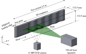
Highly controlled experiments were carried out to capture the laminar-to-turbulent transition over 2D and 3D wavy walls. The measurements were made with planar PIV in a 2.5 m long refractive-index-matching (RIM) channel with a
 $112.5\times 112.5~\text{mm}^{2}$
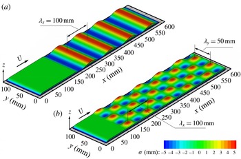
cross-section. The 2D roughness is described by a single sinusoidal wave in the streamwise direction with a ratio of amplitude to wavelength
 $a/\unicode[STIX]{x1D706}_{x}=0.05$
, while the 3D roughness is defined with an additional wave superimposed on the 2D wall in the spanwise direction with
 $a/\unicode[STIX]{x1D706}_{y}=0.1$
. The surface topography
 $\unicode[STIX]{x1D70E}(x,y)$
of both walls is illustrated in figure 1. The effect of this roughness on the boundary layer in the regime of developed turbulence at Reynolds number
 $Re=4\times 10^{4}$
(based on the bulk velocity and channel half-height) was studied by Hamed et al. (Reference Hamed, Kamdar, Castillo and Chamorro2015). They highlighted the advantage of such model in identifying the impact of the three-dimensionality of roughness on turbulent boundary layers. Both roughnesses are ‘distributed’ in the sense that they are periodic and consist of multiple peaks and troughs. Moreover, the roughness is of low order such that all peaks and troughs have the same height. For the purpose of refractive index matching, the walls were cast from urethane resins using hydrodynamically smooth moulds. NaI aqueous solution (
 ${\sim}63\,\%$
by weight,
 $\unicode[STIX]{x1D70C}=1800~\text{kg}~\text{m}^{-3}$
,
 $\unicode[STIX]{x1D708}\sim 1.1\times 10^{-6}~\text{m}^{2}~\text{s}^{-1}$
) was used as the working fluid. Through careful temperature control, the refractive index of the solution was fine-tuned to match that of the wall, rendering it nearly invisible. RIM allowed for measurements very close to the walls and within the troughs of the 3D roughness. The flow measurements were made in a streamwise wall-normal (
 $x$
–
 $z$
) plane with a spanwise location corresponding, approximately, to the channel centre (figure 2). A planar PIV system consisting of an 11 MP (
 $4000\times 2672$
pixels) CCD camera and a
 $150~\text{mJ}~\text{pulse}^{-1}$
double-pulsed laser was used, resulting in a final vector grid spacing
 $\unicode[STIX]{x0394}x=\unicode[STIX]{x0394}z=300~\unicode[STIX]{x03BC}\text{m}$
. Figure 2 shows the general schematics of the experimental set-up. The PIV system and technique used here are similar to those of Hamed et al. (Reference Hamed, Kamdar, Castillo and Chamorro2015); the reader is referred to Blois et al. (Reference Blois, Christensen, Best, Elliott, Austin, Dutton, Bragg, Garcia and Fouke2012) and Bai & Katz (Reference Bai and Katz2014) for additional details on the channel and the RIM technique.
A section of the 2D (a) and 3D (b) walls illustrating the topography of each roughness. Also shown is the elliptical inlet and the short preceding flat plate.

Schematic of the experimental set-up illustrating a section of the channel with the 2D roughness, and one of multiple fields of view (FOV).

The roughnesses were preceded by a short flat plate with an elliptical leading edge (0.18 m for the 2D and 0.1 m for the 3D). In order to capture the location of flow transition and the flow behaviour leading to it, flow measurements over the 2D wall were made in six consecutive fields of view (FOV) extending from the entrance region to
 $x/\unicode[STIX]{x1D706}_{x}=8.5$
. For the 3D roughness, flow measurements are reported in three FOVs around the location of the turbulent transition, which was found with exploratory measurements. The flow transition was studied under a free-stream velocity of
 $U_{\infty }=0.09~\text{m}~\text{s}^{-1}$
, yielding a Reynolds number based on the channel half-height
 $Re_{h}=4600$
. The roughness Reynolds number is
 $Re_{k}=U_{k}k/\unicode[STIX]{x1D708}=$
323 and 341 for the 2D and 3D roughnesses, where
 $k$
is taken as the amplitude of the roughness. The ratio of roughness height to thickness of the incoming boundary layer is
 $k/\unicode[STIX]{x1D6FF}_{99}=0.56$
and 0.6 for the 2D and 3D models. To gain further insight, the flow field over the 3D roughness was characterized at five other free-stream velocities spanning the range 0.07–
 $0.15~\text{m}~\text{s}^{-1}$
. For both roughnesses, 2000 PIV realizations were collected in each FOV. The small difference in the flat-plate length preceding the two roughnesses did not lead to significant differences as seen in
 $Re_{k}$
and
 $k/\unicode[STIX]{x1D6FF}_{99}$
. The
 $Re_{k}$
is comparable to that of Downs et al. (Reference Downs, White and Denissen2008) and Kuester & White (Reference Kuester and White2015) for the flow transition past a patch of distributed roughness. The relatively large amplitude of the roughness allows for spatially well-resolved measurements within it. However, it is important to note that, given this relatively large roughness height, the geometry of the roughness becomes a key component in defining the flow and, as such, the topography is referred to as large-scale roughness. In the literature, the effect of
 $k/\unicode[STIX]{x1D6FF}_{99}$
on the transition to turbulence is mostly encompassed in
 $Re_{k}$
. Further investigation of this effect is needed and it is the subject of current research (e.g., Bernardini et al.
Reference Bernardini, Pirozzoli, Orlandi and Lele2014). Finally, it is noteworthy that preliminary experiments over a smooth flat wall and under the same flow conditions indicated that the undisturbed flow remained laminar across the entire length of the test section.
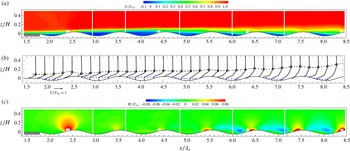
Contours (a) and profiles (b) of the time-averaged streamwise velocity
 $U/U_{\infty }$
over the 2D roughness. The white vertical strips outline the different FOVs. The dashed black line denotes
 $\unicode[STIX]{x1D6FF}_{99}/H$
and highlights the growth of the boundary layer. The dashed blue line indicates a contour line where
 $U=0$
. (c) Contours of the time-averaged wall-normal velocity
 $W/U_{\infty }$
. The small rectangular regions at the wall are due to optical obstacles outside the test section.

3 Results and discussion
3.1 Transition to turbulence over the 2D roughness
To characterize the transition to turbulence over the distributed 2D roughness, we performed extensive high-spatial-resolution PIV measurements covering a length of 0.7 m. The time-averaged distributions of the streamwise
 $U/U_{\infty }$
and wall-normal
 $W/U_{\infty }$
velocity components over this length are illustrated in figure 3. There, selected 1D profiles are also included to highlight the evolution of the mean flow. The incoming laminar boundary layer separates within the troughs, creating a region of reversed flow, which is marked with the blue dashed line in figure 3(b). This region occupies the majority of the second and third troughs; however, it significantly reduces downstream, where the flow begins the transition to turbulence. As shown below in figure 5, the flow is in the transitional regime within
 $4\lesssim x/\unicode[STIX]{x1D706}_{x}\lesssim 6$
and becomes turbulent at
 ${\sim}6\unicode[STIX]{x1D706}_{x}$
or 0.6 m from the leading edge (
 $Re_{x}=U_{\infty }x/\unicode[STIX]{x1D708}=5\times 10^{4}$
). In the laminar region (
 $x/\unicode[STIX]{x1D706}_{x}\lesssim 4$
), the roughness seems to have a comparatively less significant role in modulating the flow, as suggested by the distribution of the vertical velocity
 $W/U_{\infty }$
. A region of comparatively high upward flow occurs at the first roughness peak; otherwise the wall-normal velocity is significantly lower than that within the turbulent region
 $x/\unicode[STIX]{x1D706}_{x}\gtrsim 6$
(figure 3
c). A negligible flow of momentum occupies the majority of the troughs within the laminar region and results in the upward displacement of the boundary layer. Drews (Reference Drews2012), in his DNS study of 3D distributed roughness, replaced the troughs with a streamwise and spanwise slip surface to understand the effect of roughness ‘valleys’. He found that the flow downstream is unaffected, and suggested that roughness valleys do not significantly contribute to receptivity. A somewhat similar behaviour is observed here for the 2D roughness, where the recirculation within the valleys in the laminar regime (
 $x/\unicode[STIX]{x1D706}_{x}\lesssim 4$
) acts as a blockage, reducing wall-normal flows and possibly minimizing vortical shedding from the 2D hills.
Mean shear
 $\unicode[STIX]{x2202}(U/U_{\infty })/\unicode[STIX]{x2202}(z/H)$
over a section of the 2D roughness covering the transitional and turbulent regions.

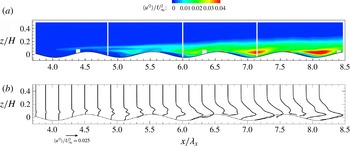
Contours (a) and profiles (b) of the streamwise velocity variance
 $\langle {u^{\prime }}^{2}\rangle /U_{\infty }^{2}$
over a section of the 2D roughness covering the transitional and turbulent regions.

However, a major difference from the work of Drews (Reference Drews2012) is the disturbances created by the separated flow within the 2D roughness troughs. The recirculation region enables an inflection point in the boundary layer profile that corresponds to a maximum in the mean shear
 $\unicode[STIX]{x2202}(U/U_{\infty })/\unicode[STIX]{x2202}(z/H)$
shown in figure 4. For
 $x/\unicode[STIX]{x1D706}_{x}\lesssim 4.5$
, the boundary layer profile exhibits an inflection point with a mean shear maximum that is thought to promote flow instability, leading to the peak in the streamwise velocity variance
 $\langle {u^{\prime }}^{2}\rangle /U_{\infty }^{2}$
, which is shown, for clarity, as contours and profiles in figure 5. This quantity reveals that the region
 $x/\unicode[STIX]{x1D706}_{x}\lesssim 4$
has negligible fluctuations and is identified as the laminar regime, whereas for
 $x/\unicode[STIX]{x1D706}_{x}\gtrsim 6$
the flow exhibits spatially distributed turbulent fluctuations similar to that observed by Hamed et al. (Reference Hamed, Kamdar, Castillo and Chamorro2015) in a developed flow, and is thus identified as the turbulent regime. There, the production of turbulence is attributed to the shear layer formed behind the roughness crests. The intermediate zone
 $4\lesssim x/\unicode[STIX]{x1D706}_{x}\lesssim 6$
is considered, consequently, to be a transitional region. Within this zone, the fluctuations are contained in a narrow band (
 $4\lesssim x/\unicode[STIX]{x1D706}_{x}\lesssim 4.7$
) above the roughness with peak at
 $z/H=0.08$
–0.1 coincident with a peak in the mean shear associated with the mean velocity inflection. The fluctuations in this region possibly trigger disturbances near the roughness. The crest near
 $x/\unicode[STIX]{x1D706}_{x}=4.5$
develops a shear layer, which leads to additional velocity inflection points that explain the two shear and velocity variance peaks observed within the transitional region (figures 4 and 5). The near-roughness fluctuations quickly over take those related to the displaced boundary layer. However, in the transitional region the two mechanisms interact and lead to rapid vertical growth of the velocity fluctuations.
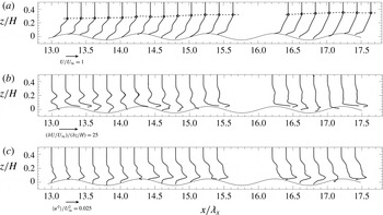
(a) Profiles of time-averaged streamwise velocity
 $U/U_{\infty }$
over a section of the 3D roughness. The dashed black line denotes
 $\unicode[STIX]{x1D6FF}_{99}/H$
. (b,c) The corresponding profiles of the mean shear
 $\unicode[STIX]{x2202}(U/U_{\infty })/\unicode[STIX]{x2202}(z/H)$
and the streamwise velocity variance
 $\langle {u^{\prime }}^{2}\rangle /U_{\infty }^{2}$
.

3.2 Transition to turbulence over the 3D roughness
The characterization of the transition to turbulence over the distributed and low-order 3D roughness provides important insight into the case where the steady disturbances (wakes) are created over an array of compact elements covering the entire domain. This advances the work of Downs et al. (Reference Downs, White and Denissen2008) and Kuester & White (Reference Kuester and White2015), who studied the downstream evolution of disturbances created over a short roughness patch. Moreover, due to the similar experimental conditions, free-stream velocity
 $U_{\infty }=0.09~\text{m}~\text{s}^{-1}$
and
 $Re_{k}\approx 300$
, the results presented here provide a meaningful comparison between flow transition over the periodic 2D and 3D roughnesses. The flow over the 3D roughness reaches its turbulent behaviour at 1.5 m (
 $Re_{x}=1.2\times 10^{5}$
) from the leading edge in comparison with 0.6 m (
 $Re_{x}=5\times 10^{4}$
) for the 2D wall, i.e., 2.5 times longer. Therefore, we focus on the mean streamwise velocity
 $U/U_{\infty }$
, the mean shear
 $\unicode[STIX]{x2202}(U/U_{\infty })/\unicode[STIX]{x2202}(z/H)$
and the streamwise velocity variance
 $\langle {u^{\prime }}^{2}\rangle /U_{\infty }^{2}$
within the transitional and turbulent regions, which are shown in figure 6. The lack of mean flow reversal within the troughs is due to the preferential flows identified by Hamed et al. (Reference Hamed, Kamdar, Castillo and Chamorro2015), which inject momentum into the wakes of the 3D hills. The flow field is best analysed in the context of the work by Ergin & White (Reference Ergin and White2006), Downs et al. (Reference Downs, White and Denissen2008) and Kuester & White (Reference Kuester and White2015). There, it is shown that, as the undisturbed boundary layer flow passes roughness elements, the formed steady disturbances (wakes) lift up downstream, experience transient growth and promote velocity fluctuations. The transition to turbulence occurs when the fluctuations grow rapidly before the unstable steady state can relax to a stable one. Here, the process is different because steady disturbances (wakes) are generated along the entire flow domain at each element of the roughness array. These steady disturbances lift up and likely interact over the length of the roughness array, leading to the mean velocity deficit at
 $0.08\lesssim z/H\lesssim 0.25$
(figure 6
a). Consequently, it is challenging to uncouple the contribution of the generation from the growth/decay. Therefore, the systematic velocity deficit observed in figure 6(a) is an aggregation of both.
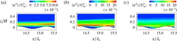
Contours of the streamwise velocity variance
 $\langle {u^{\prime }}^{2}\rangle /U_{\infty }^{2}$
for the 3D wall at
 $14.2\leqslant x/\unicode[STIX]{x1D706}_{x}\leqslant 15.5$
for different free-stream velocities. (a)
 $U_{\infty }=0.07~\text{m}~\text{s}^{-1}$
, (b)
 $U_{\infty }=0.09~\text{m}~\text{s}^{-1}$
, (c)
 $U_{\infty }=0.16~\text{m}~\text{s}^{-1}$
.

The velocity deficit at
 $0.08\lesssim z/H\lesssim 0.25$
(figure 6) corresponds to a region of enhanced shear and fluctuations with local peaks near
 $z/H=0.2$
. High mean shear and comparatively larger velocity fluctuations are also induced near the roughness. These fluctuations overtake those related to the steady disturbances. However, they interact similarly to the 2D case, leading to rapid vertical growth of the fluctuation distribution. The steady disturbances and their corresponding shear rapidly decay due to turbulent mixing at
 $x/\unicode[STIX]{x1D706}_{x}\gtrsim 15$
. To further highlight the effect of this interaction, we show in figure 7 contours of the streamwise velocity variance
 $\langle {u^{\prime }}^{2}\rangle /U_{\infty }^{2}$
in the region
 $14.2\leqslant x/\unicode[STIX]{x1D706}_{x}\leqslant 15.5$
for three free-stream velocities (
 $U_{\infty }=0.07~\text{m}~\text{s}^{-1}$
,
 $U_{\infty }=0.09~\text{m}~\text{s}^{-1}$
,
 $U_{\infty }=0.16~\text{m}~\text{s}^{-1}$
). When considering the location of flow transition, the lower (higher) free-stream velocity is somewhat analogous to moving the measurement region upstream (downstream). At the lowest velocity, only the fluctuations associated with the steady disturbances are present. At the highest velocity, the flow is in its turbulent regime where the turbulence is generated by the shear layer downstream of the hills, similar to the findings of Hamed et al. (Reference Hamed, Kamdar, Castillo and Chamorro2015). The case with
 $U_{\infty }=0.09~\text{m}~\text{s}^{-1}$
shows the transitional region where both generation mechanisms are present and manifested in rapid vertical growth of the fluctuation distribution (also seen in the profiles of figure 6
c). Additionally, snapshot proper orthogonal decomposition (POD) analysis was performed following Sirovich (Reference Sirovich1987) on a subset of 1000 fluctuating velocity fields for these three cases. POD is used to extract the dominant spatial features of the flow by decomposing the fluctuating velocity signal
 $\boldsymbol{u}^{\prime }(\boldsymbol{x},t)$
into a deterministic part
 $\unicode[STIX]{x1D753}^{n}(\boldsymbol{x})$
(POD modes) and time-dependent coefficients
 $a^{n}(t)$
as
 $$\begin{eqnarray}\boldsymbol{u}^{\prime }(\boldsymbol{x},t)=\mathop{\sum }_{n=1}^{1000}a^{n}(t)\unicode[STIX]{x1D753}^{n}(\boldsymbol{x}).\end{eqnarray}$$
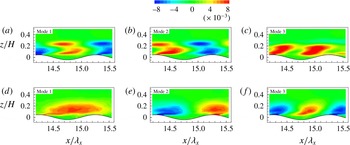
For a more detailed description of POD, the reader is referred to the work of Lumley (Reference Lumley1970), Sirovich (Reference Sirovich1987) and Berkooz, Holmes & Lumley (Reference Berkooz, Holmes and Lumley1993). Figure 8 shows the first three modes of the streamwise velocity fluctuations
 $\unicode[STIX]{x1D719}_{u^{\prime }}$
for the two higher free-stream velocities. For the case of
 $U_{\infty }=0.16~\text{m}~\text{s}^{-1}$
, the three modes contain 23 % of the total energy of all modes and are in agreement with Hamed et al. (Reference Hamed, Kamdar, Castillo and Chamorro2015). For the case of
 $U_{\infty }=0.07~\text{m}~\text{s}^{-1}$
(omitted here for brevity), the first mode showed a band similar to that observed in the streamwise velocity variance and contributed 80 % of the total energy. The case of interest is
 $U_{\infty }=0.09~\text{m}~\text{s}^{-1}$
, where the three modes shown contribute 36 % of the total energy but do not resemble those in the turbulent regime. The spatial structures exhibit different scales and show an interaction between the region away from the wall, which is influenced by the steady disturbances, and structures near the wall, which are influenced by the topography. Finally, it is worth pointing that similar behaviour and energy content were observed in the POD modes for the 2D case in the transitional region.
Figures 5 and 7 highlight the difference in the nature of the transitional region across the two roughnesses. For the 2D case, the narrow band of high velocity variance in the region
 $4\lesssim x/\unicode[STIX]{x1D706}_{x}\lesssim 4.7$
is associated with the velocity inflection point as discussed above. In the 3D case, the wider band is associated with the velocity deficit region originating from the interaction of the wakes of upstream elements. The rapid vertical growth of the fluctuation distribution is a common feature of the transition region across both roughnesses. The generation of shear layer turbulence in the turbulent region is another common feature (Hamed et al.
Reference Hamed, Kamdar, Castillo and Chamorro2015).
POD modes of the streamwise velocity fluctuations
 $\unicode[STIX]{x1D719}_{u}^{\prime }$
for
 $U_{\infty }=0.09~\text{m}~\text{s}^{-1}$
(a,b,c) and
 $U_{\infty }=0.16~\text{m}~\text{s}^{-1}$
(d,e,f).

4 Conclusions
The transition to turbulence over 2D and 3D roughness was studied experimentally using planar PIV and refractive index matching. The topography covered the entire flow domain, which complements previous works that studied the disturbances created by a short roughness patch (e.g., Downs et al.
Reference Downs, White and Denissen2008; Kuester & White Reference Kuester and White2015). The recirculation within the troughs of the 2D roughness facilitates the vertical displacement and growth of the boundary layer over the roughness. However, an inflection point in the displaced boundary layer profile promotes high shear and fluctuations that occur in the region above the roughness. For the 3D topography, the flow transition is significantly delayed (
 $Re_{x}=120\,000$
versus the 50 000 of the 2D case). In the transitional region, the interaction of the wakes of upstream elements is manifested in a deficit in the mean streamwise velocity profile above the roughness. The significant delay in flow transition over the 3D roughness is attributed to the spanwise flows within the topography (measured by Hamed et al. (Reference Hamed, Kamdar, Castillo and Chamorro2015)), which reduce the likelihood of flow separation (and, consequently, velocity inflection points) by injecting high-momentum fluid in the wakes of the 3D hills. Within the transitional region fluctuations are initially observed above the roughness and are due to the inflection point of the displaced boundary layer for the 2D case and the velocity deficit for the 3D case. These above-roughness disturbances are thought to trigger additional disturbances near the roughness. The above- and near-roughness regions of enhanced mean shear and fluctuations interact, leading to rapid vertical growth of the turbulent fluctuations.
Acknowledgements
This work was supported by the Department of Mechanical Science and Engineering, University of Illinois at Urbana-Champaign, as part of the start-up package of L.P.C. The experiments were performed in a facility built under the National Science Foundation grant award CBET-0923106. The authors are grateful for the help of undergraduate students A. Patkar and D. Harmon at the University of Illinois.